Innovative Actuator Fault Identification Based on Back Electromotive Force Reconstruction


Department of Aerospace and Mechanical Engineering (DIMEAS), Politecnico di Torino, 10129 Turin, Italy
*
Author to whom correspondence should be addressed.
Actuators 2020, 9(3), 50; https://0-doi-org.brum.beds.ac.uk/10.3390/act9030050
Submission received: 21 May 2020
/
Revised: 27 June 2020
/
Accepted: 1 July 2020
/
Published: 3 July 2020
(This article belongs to the Section Aircraft Actuators)
Abstract
:The ever increasing adoption of electrical power as secondary form of on-board power is leading to an increase in the usage of electromechanical actuators (EMAs). Thus, in order to maintain an acceptable level of safety and reliability, innovative prognostics and diagnostics methodologies are needed to prevent performance degradation and/or faults propagation. Furthermore, the use of effective prognostics methodologies carries several benefits, including improved maintenance schedule capability and relative cost decrease, better knowledge of systems health status and performance estimation. In this work, a novel, real-time approach to EMAs prognostics is proposed. The reconstructed back electromotive force (back-EMF), determined using a virtual sensor approach, is sampled and then used to train an artificial neural network (ANN) in order to evaluate the current system status and to detect possible coils partial shorts and rotor imbalances.
1. Introduction
In the last decade there has been increased shift from traditional, hydraulic actuators to electric actuators, due to the progressive adoption of the more electric [1] and all electric design philosophies. In these design approaches electrical energy is the privileged form of secondary power used to drive subsystems and utilities. The natural interface with mechanical systems is the electromechanical actuator (EMA), that, in its simplest form, is an electric motor connected via one or more reduction stages to the element that needs to be actuated. In civil liners, the shift has been limited to secondary flight controls (e.g., flaps, slats, airbrakes), while safety-critical systems such as primary flight controls and landing gears actuators still use traditional hydraulic-based devices in the form of hydromechanical or electrohydrostatic actuators as in the Airbus A400 series [2].
The choice has two main reasons: hydraulic-based actuators are still more compact and lighter than the electric counterpart; at the same time, failure modes of hydraulic actuators are well studied given the extensive adoption for primary flight controls, while EMAs have seen little operative service as primary actuation devices, despite the widespread adoption in other sectors (e.g., manufacture and industrial automation); consequently, failure modes of EMAs are relatively well understood, as reported in [3]. Nevertheless, the lack of an extensive failures data set in operating conditions is a major setback for their adoption, given the potential severity and criticality of some failure modes [4]. Furthermore, the data obtained for secondary controls actuation is not directly translatable to primary controls application, given the very different command and actuation schemes for the two roles [2]. To allow the use of EMAs as primary flight controls actuators and for other safety-critical operations, a proper prognostic and health management (PHM) methodology needs to be implemented, besides a rapid and effective Fault Detection and Identification.
A definition is given in [5] as "prognostics and health management" (PHM) refers specifically to the phase involved with predicting future behavior, including remaining useful life (RUL), in terms of current operating state and the scheduling of required maintenance actions to maintain system health"; effective PHM can be achieved using three different approaches, i.e., data-driven prognostics, model-based prognostics and hybrid approaches.
Data-driven prognostics leverages pattern recognition and machine learning tools such as neural networks and neural fuzzy networks [6]. The scope is to detect alteration in the system state and to link such changes to some kind of fault (classification), or even estimate the magnitude of the defects (regression); in general, classification problems are easier to tackle and thus most of the analyses focuses on classification rather than regression, as reported in [7] in regards to wind turbines condition monitoring. The advantage of the approach is the ample scope of the analysis, since there is no need to accurately model the system in examination; however, a large data set and powerful hardware is necessary to obtain accurate data in a reasonable time frame.
On the other hand, model-based prognostics is based on a mathematical representation of the component or system studied using a set of differential equation describing the temporal evolution of the system, as in [8,9]. The advantage of the approach is the ability to precisely describe the behavior of an element allowing for a very precise fault detection. Furthermore, the fault propagation is generally embedded in the model, enabling the estimation of how such fault will propagate under given operating conditions. However, creating detailed and precise models for complex systems like aeronautical systems is time consuming and usually requires the simplified modeling of hard-to-simulate phenomena, e.g., aerodynamics, usually resulting in a degraded simulation accuracy.
Finally, hybrid approaches try to merge the strength of both methods, i.e., speed and accuracy, respectively, using machine learning tools applied to mathematical models representing the analyzed system or component. Two categories of hybrid approaches exist: pre-estimate fusion and post-estimate fusion. Further details can be found in [10,11,12,13].
Regarding practical PHM implementation in aeronautical systems, several solutions are being studied, as in [14], where permanent magnet synchronous motors interturn failures have been estimated using residual analysis; in [15] various optimization techniques, based on genetic algorithms, are presented in order to estimate and identify degradation levels in EMAs, extending the work presented in [16]; more examples of manufacture-based PHM works include [17,18].
Another important aspect of effective prognostics is the estimation of the Remaining Useful Life (RUL), that is an indicator of the time left before the component or system will not comply to the imposed requirements. Many works have focused on RUL estimation, generally leveraging machine learning techniques such as Artificial Neural Networks (ANNs) in various forms, such as deep convolution networks in [19], semi-supervised deep architectures as in [20], recurrent neural networks in [21], long short-term memory (LSTM) networks in [22], deep LSTM in [23], bidirectional handshaking LSTM as in [24], multimodal and hybrid networks as in [25] or even a fusion of neural networks and Kalman filters as in [26,27]; statistical methods are also effectively adopted as in [28] where discrete-time Markov chains are used to estimate RUL for components with time-varying operational conditions or in [29] where Bayesian inference is applied to estimate air conditioning units health state. One of the problem that arises in RUL estimation is the intrinsic uncertainty of the degradation dynamics; this phenomenon can be mitigated by using particle filters, as presented in [30]; another development, presented in [31], suggest a more complex approach which includes the modeling of the degradation trend.
In this work, a novel methodology for EMAs prognostics will be presented. Using a detailed MATLAB Simulink model of an EMA actuating a flaperon, taken from [32], the reconstructed back electromotive force (back-EMF), calculated as in [33], is firstly sampled and then used to evaluate the status of the system in order to identify two different kinds of faults, i.e., partial coils shorts and rotor static eccentricity, leveraging feedforward neural networks.
2. Materials and Methods
2.1. Scope of The Work
The aim of the work is to present a novel prognostic methodology, based on the reconstruction of the back-EMF coefficient curve, for electromechanical actuators. The novelty is in the use of a mapping signal, which in this case is the back-EMF coefficient, in order to create a separation between signals time series, widely used in current prognostic methods, and the neural network. Mapping signals must express two characteristics: strong correlation with faults of interest and low sensitivity to operating and environmental conditions. In this case, the back-EMF coefficient is a good candidate regarding phase partial shorts and static eccentricity faults, since these faults strongly affect the signal while command inputs and external loads do not, as demonstrated in [33].
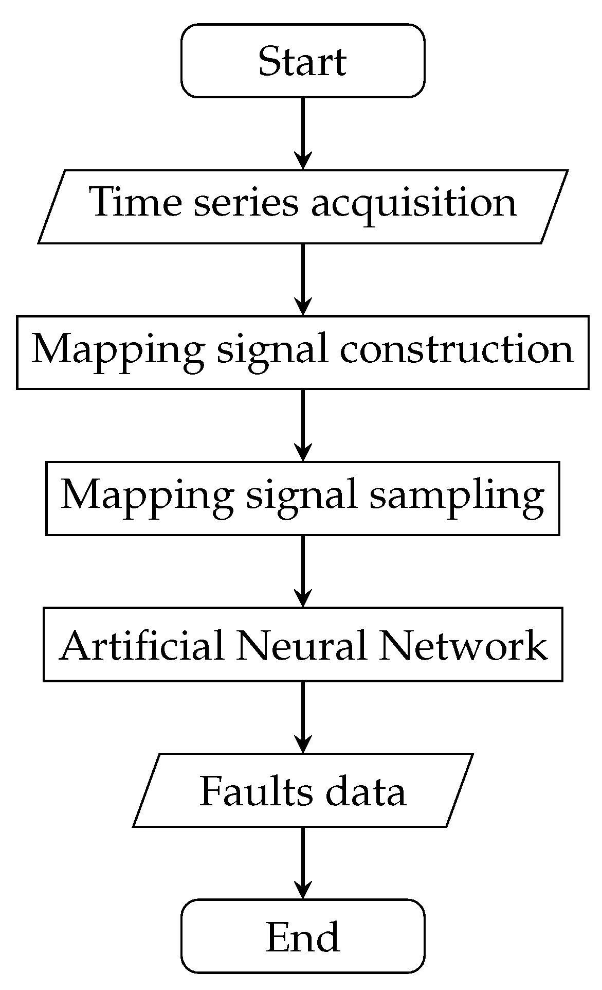
After the mapping signal has been reconstructed, it is opportunely sampled and machine learning (i.e., ANNs) is then used to perform a regression and thus evaluate system faults levels. A graphical form of the algorithm is presented in Figure 1.
The algorithm does not operate in a continuous manner; the faults data returned as outputs represent system degradation at that particular epoch. Nonetheless, the algorithm can be run whenever an estimation of system health is necessary. Furthermore, the faults data can be used to estimate the RUL of the system (e.g., using regression), even tough this particular aspect is not covered in this paper.
Traditional fault detection approaches for servosystems are only applicable if the actuation time history is repeatable. The advantage of the method proposed in this work is the applicability to systems where an inherent uncertainty on external load or actuation command is present, such as aerospace actuators.
Since the core of the methodology is based on the construction of a mapping signal, it can be easily adapted to other types of servosystems; the problem is now shifted on the determination of an appropriate mapping signal that respects the two characteristics previously described; the rest of the algorithm remains then unchanged.
2.2. Model Overview
In this work, an aerospace EMA model has been chosen as test case application for the algorithm; as previously stated, an apt signal for this type of actuators is the back electromotive force (back-EMF) coefficient, as reported in [33]. It has to be noted the model is not directly part of the prognostics method; in fact, the main function of the model is to simply verify the application of the algorithm in a reasonably realistic application.
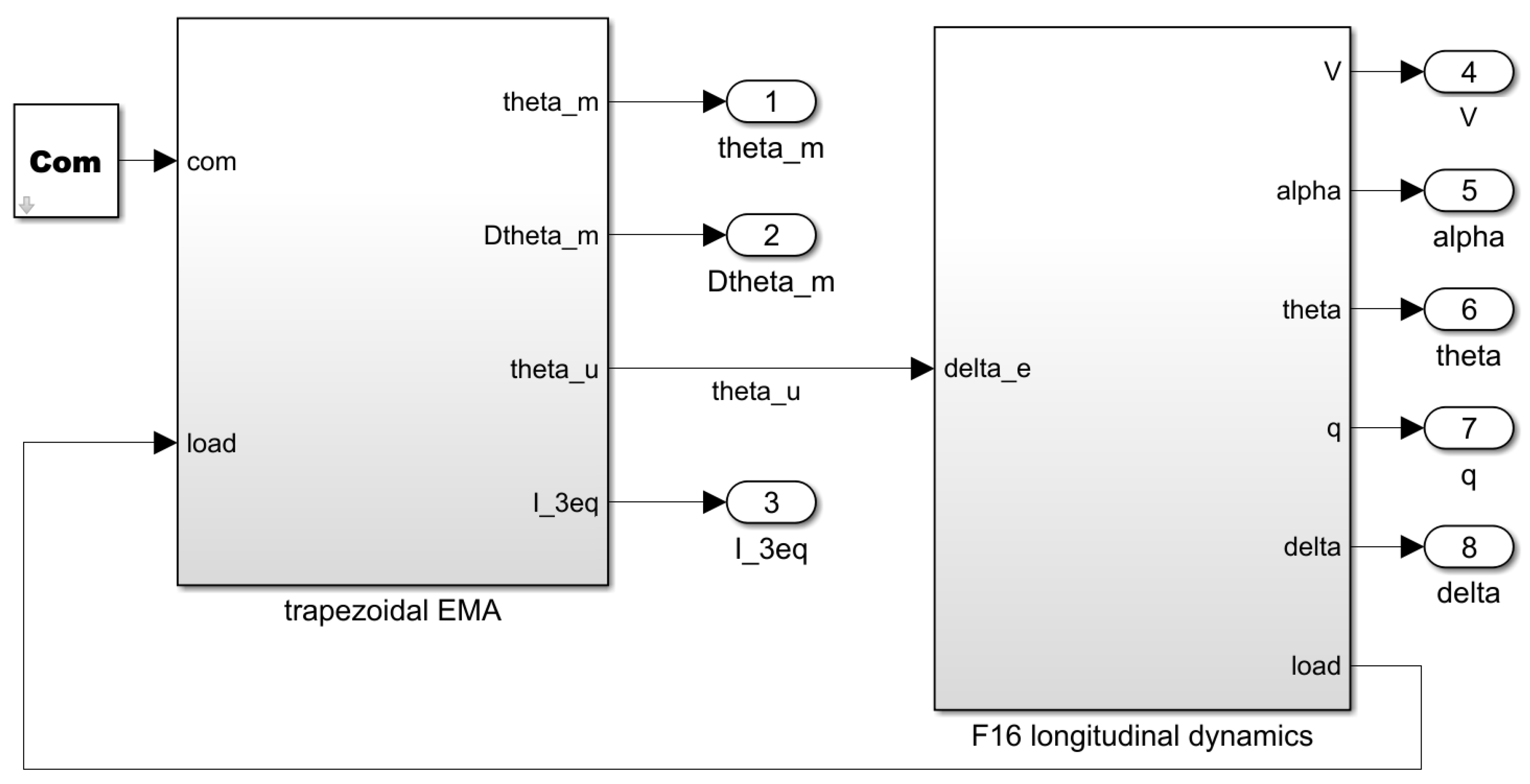
The Simulink model used to generate the data set is taken from [32], so only a brief description will be presented in this paper. The top level view (Figure 2) shows two subsystems, i.e., the trapezoidal EMA assembly on the left and the simplified F16 longitudinal dynamics on the right. A feedback loop is present between the two subsystems, that is the load acting on the aerodynamic surface. The leftmost element, the Com block, is used to impose a particular position command (e.g., step, ramp, sinusoidal etc.) to the surface.
The relevant logged signals are motor angular position, , motor angular speed, and the single-phase equivalent instantaneous current, ; the relevant aerodynamic parameters are angle of attack, , pitch angle , angular rate q, surface deflection and aircraft speed V.
2.3. Trapezoidal EMA
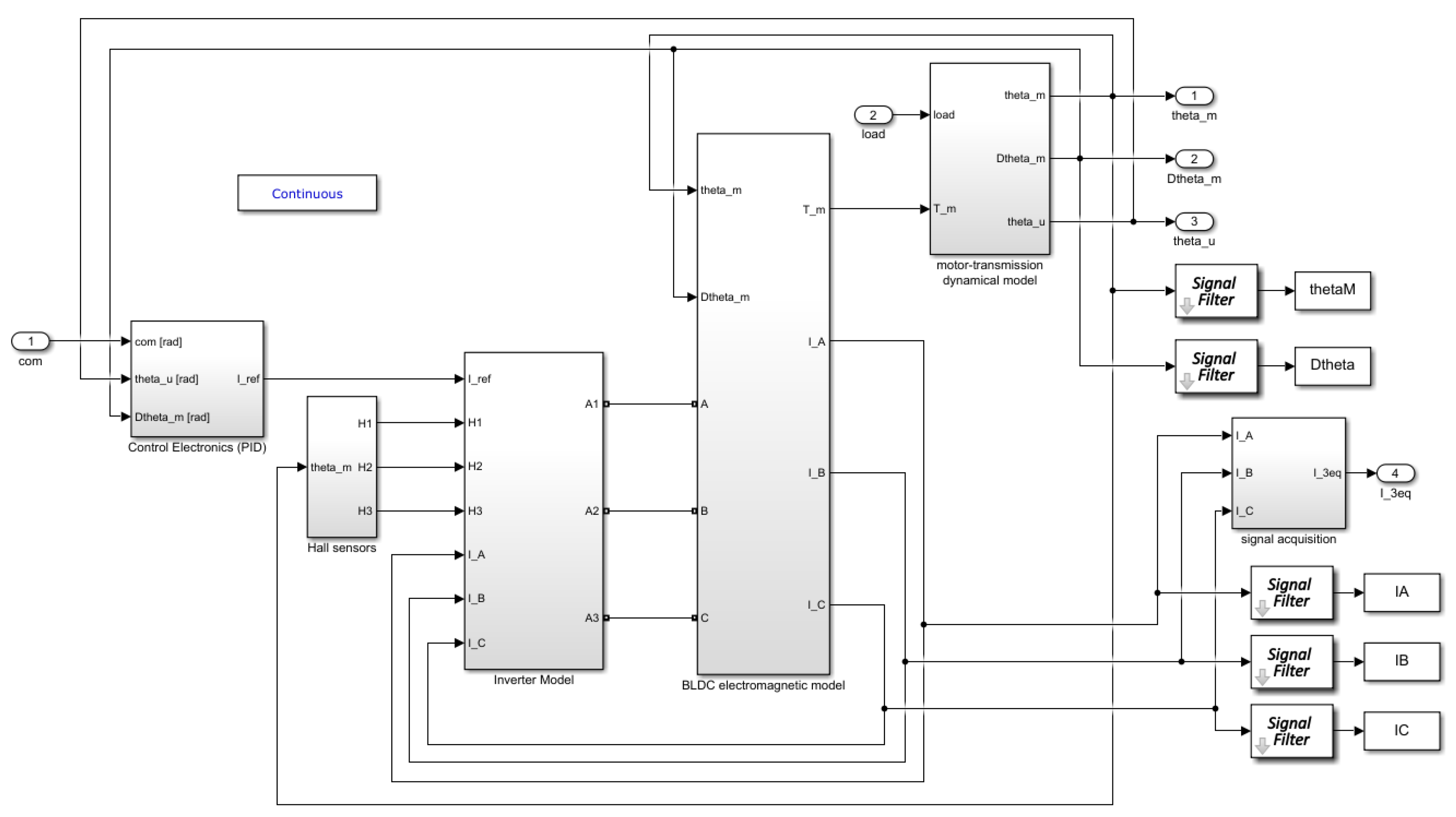
The expanded trapezoidal EMA is shown in Figure 3 and will be shortly described.
The leftmost subsystem was a control electronics subsystem, i.e., a Proportional Integral Derivative (PID) controller receiving as inputs the commanded position, the user position and angular speed; the output, i.e., the reference current was needed to achieve the required position.
The following subsystem modeled the Hall sensors present in a Brushless Direct Current (BLDC) motor that were of fundamental importance to the operation since they were necessary to determine the rotor angular position and thus activate the commutation scheme using three different signals, i.e., and by using a commutation table based on rotor angular position.
The inverter model used Simscape components to model a classical DC-AC inverter using a PWM controller. It received the reference current elaborated by the controller, the three commutation signals evaluated by the Hall sensors block and three phases currents (, and ) as feedback loops. The outputs, , and were Simscape physical connections to the EM model.
The BLDC electromagnetic model once again used Simscape electrical elements, particularly RL (Resistor, R and Inductor, L) branches, to model the three phases of the BLDC motor itself. The inputs were the three aforementioned electrical connections with the inverter and motor position and speed in order to evaluate viscous effects. The outputs were the three phases currents , and and the motor torque, .
Finally, the motor-transmission dynamical models represented the mechanical linkage between the motor and the surface; in particular, a single stage reduction gear was modeled. The inputs were the motor torque and external load, while the outputs were motor position and speed, and respectively and user angular position, . Further details can be found in [32].
The signal acquisition block was used to save the three phases currents data (i.e., , and ) as a single-phase equivalent current to MATLAB workspace.
2.4. F16 Longitudinal Dynamics Model
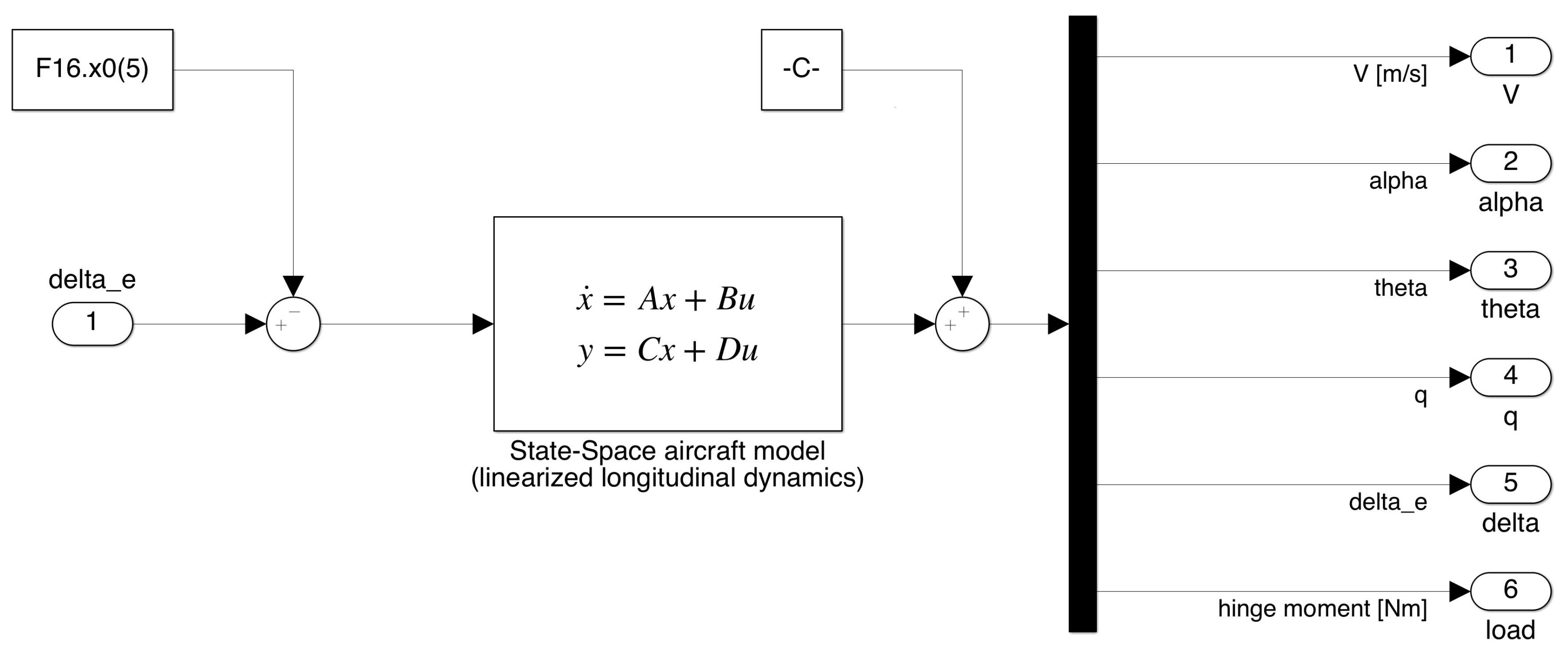
The longitudinal dynamics model (Figure 4) of the aircraft is a simple state-space linearization, taken from [34]. The inputs to the state-space model were delta_e, that is the elevator deflection angle, while the constant block -C- contained the initial conditions. The block F16.x0(5) represented the trim angle.
Model outputs were speed V, angle of attack , pitch angle , pitch rate q, elevator deflection and hinge moment.
2.5. Faults Generation
An extensive data set was obtained using the faults generation scheme presented in [33]. Basically, the approach used an exponentially scaled, 5-dimensional Latin hypercube method to obtain an exponentially spaced fault vector.
Each fault vector had the following form:
where and represent a percentage coil short for each phase, so their value is bounded to the interval , where 0 means no damage and 1 represents a total phase short.
The parameter is used to define static eccentricity as where is the axis offset from center and is the nominal air gap. Finally, represents the angular phase of the static eccentricity.
Furthermore, two limits were set in order to simulate only realistic prognostics (and not diagnostic) conditions, i.e., conditions where the system could still achieve the imposed requirements albeit with degraded performance, by using the following two equations:
The values chosen for the previous equations are arbitrary, even tough they hold a physical significance. As previously stated, such boundaries are used to limit simulation cases to prognostic conditions, and not to analyze diagnostic conditions where other safety systems would act. Precise values for the previous equations can be empirically evaluated using a real system, setting a cut-off point for prognostics when the system does not comply anymore to imposed requirements (e.g., frequency response). In any case, the exact numerical values did not affect the operation of the prognostic algorithm.
2.6. Back-EMF Reconstruction
The back-EMF reconstruction procedure was the one presented in [33], so it will be described briefly. Having logged the relevant signals, i.e., three phase currents, three phase voltages, motor angular position and speed, the following electrical equation describes the system:
where is the counter electromotive force for each motor phase. Considering that , solving for the back-EMF coefficient yields:
where j represents one of the three phases and and are motor nominal phase resistance and inductance, respectively.
Having obtained the back-EMF as function of the timestep, it is then resampled and correlated with motor angular position using the following equation:
where is the semi-amplitude of a tolerance band centered on .
Finally, the equivalent single-phase back-EMF coefficient is obtained by
The equivalent back-EMF coefficient signal, now a function of the rotor angle, is ready to be sampled.
2.7. Curves Sampling
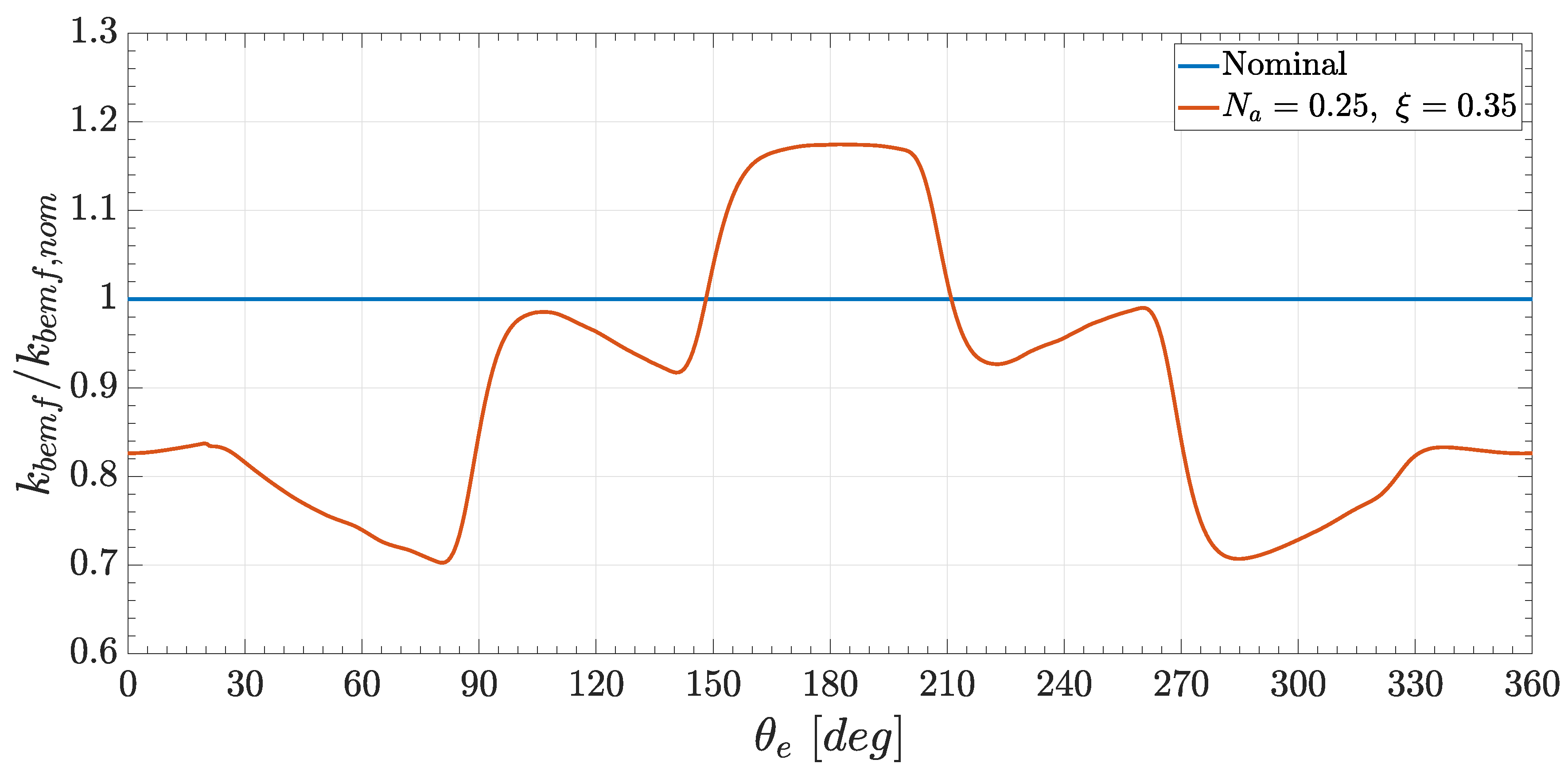
The reconstructed back-EMF coefficient curve had a certain regularity given by the periodicity of the commutation events taking place every 30 electrical, as clearly visible in Figure 5. This regular behavior could be exploited to implement several sampling techniques. Three different methodologies were analyzed, differing in the number of sample points extrapolated for each period between two successive commutations (intracommutation period).
The first sampling mode extrapolated the center point value of each intracommutation period, for a total of six points per each curve, i.e., per single faults combination; the central point was sampled assuming that the commutations were instantaneous and only spanned a single timestep.
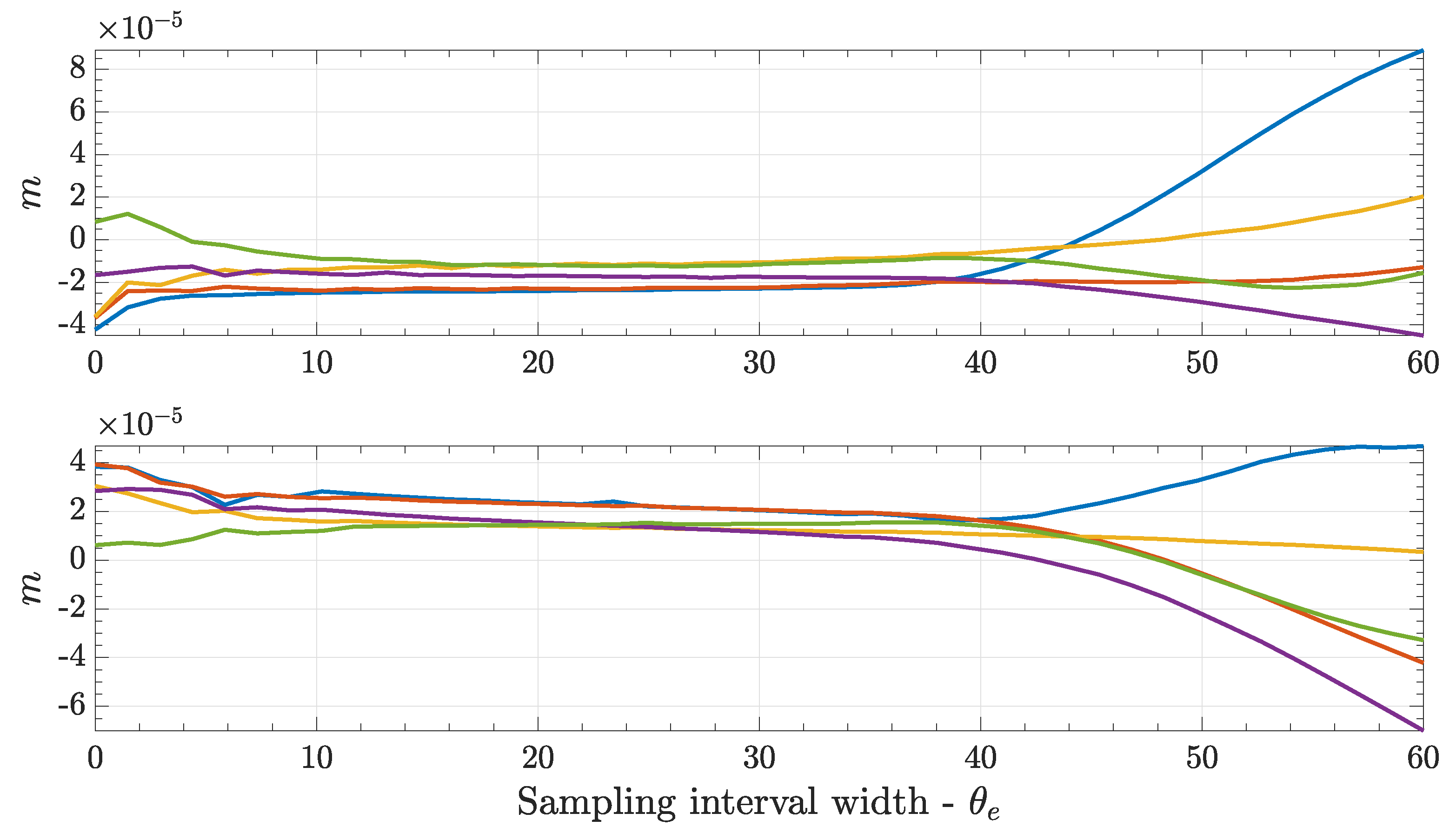
The second sampling mode instead sampled two different points for each intracommutation period, for a total of 12 points per back-EMF coefficient curve. In this case, there was a need to take into account the noise present in the signal, even tough the reconstructed signal used filtered signals. By using a linear interpolation, in the form per each intracommutation phase, the maximum angular range where the the curve could be approximated as linear before commutation effects manifested was determined. In particular, in Figure 6, the zone where there was no variation in the angular coefficient of the interpolating line as function of the considered interval amplitude is shown. This was a necessary step since the value could greatly differ if the values were sampled in proximity of a commutation and, on the other side, a too small interval could be affected by local noise. Thus an angular amplitude of 20 electrical was chosen (i.e., ±10 electrical in respect to the midpoint of the intracommutation period), considering a total angular range of 60 electrical between two successive commutations.
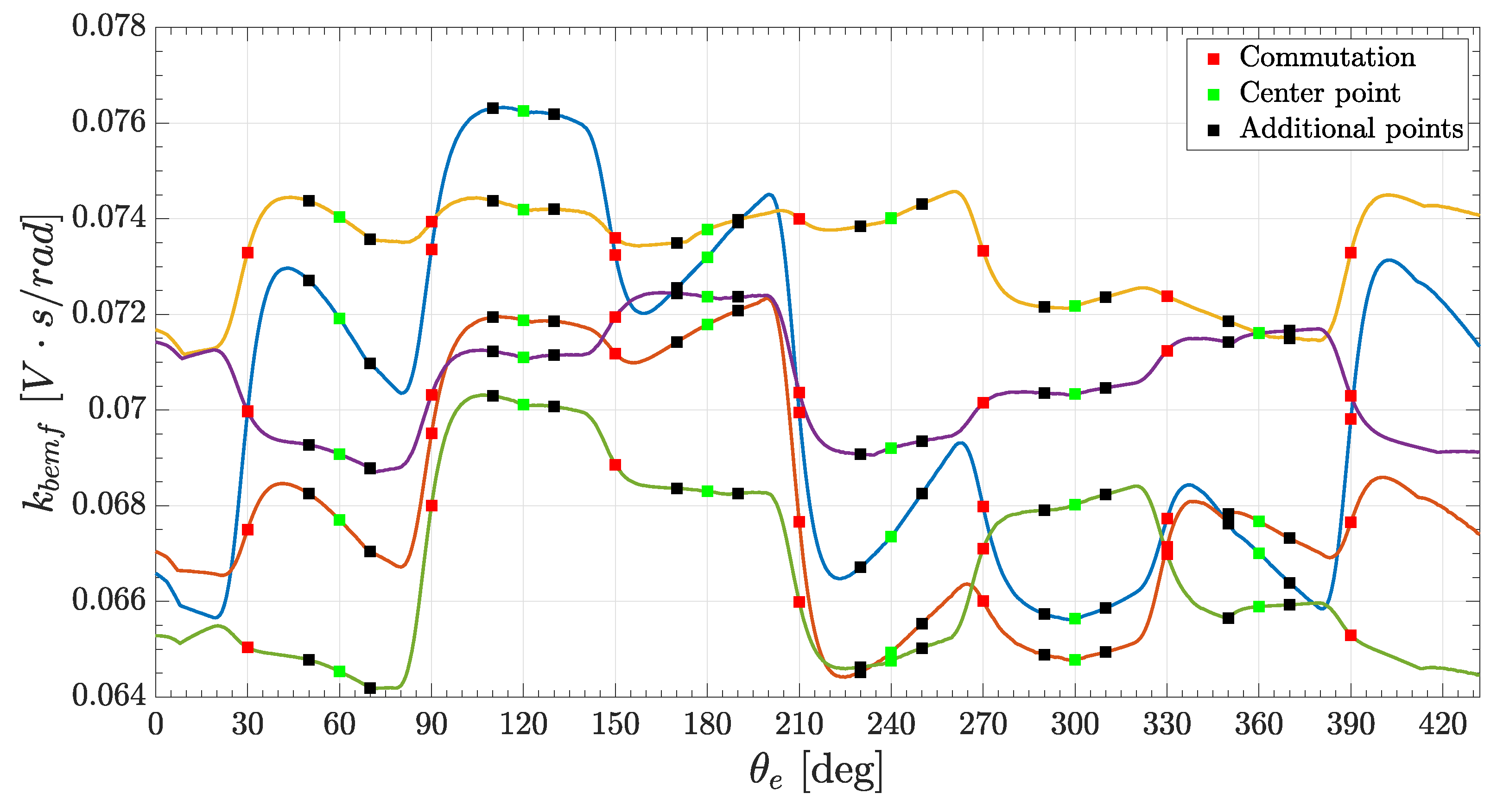
Finally, the third sampling mode was a fusion of the previous two methods, i.e., a combination of center point and two additional points per intracommutation period, for a total of 18 points per each curve. In Figure 7 the relevant points (commutations, center points and additional points) are shown for five randomly seeded curves.
2.8. Neural Networks Description
Artificial neural networks (ANNs) are a powerful machine learning tool. The name is a reflection on the principle of operation, resembling biological neural networks; the system ’learns’ to perform different tasks based on examples, generally without specific programming rules. The scope of a neural network is to fit data that would be impractical to elaborate using other methods (e.g., many-dimensional data set fitting, image classification, speech recognition, etc.).
Network structure is based on a series of fundamental elements, neurons, opportunely connected to others, in similarity to biological synapses; the individual combination of neurons and connections uniquely defines the topology. Each connection has an associated weight, representing its relative importance; weights values are modified during training in order to minimize the error function defined for the task using a training function, generally leveraging a back-propagation method. Several learning paradigms exist, such as supervised, unsupervised and reinforcement learning, where each is more performing for a particular task (e.g., supervised learning for pattern recognition).
Another important characteristics defining the network is the propagation function, used to evaluate neuron inputs based on connected predecessor neurons outputs as a weighted sum; optionally, a bias term can be included as an additional parameter to each neuron, increasing network complexity and capabilities.
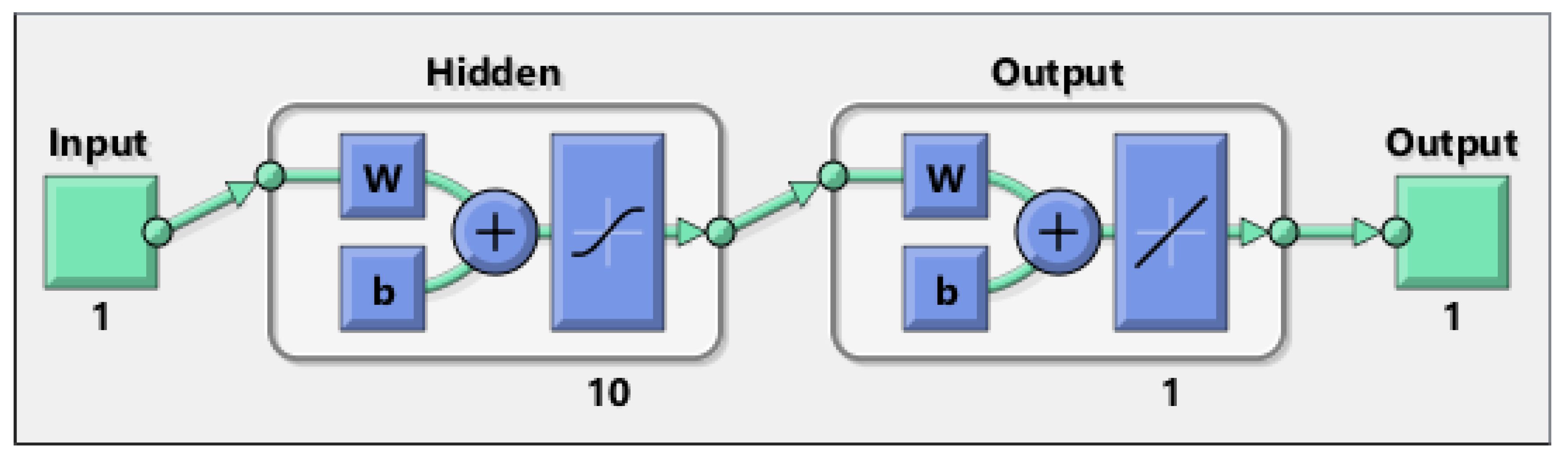
In this work, networks were implemented using MATLAB Machine Learning Toolbox. The architecture for all networks was either a single layer or two layer perceptron (Figure 8), i.e., having either one or two hidden layers. Networks inputs were the previously sampled values as described in Section 2.7, while the outputs were always five for every network configuration, representing the target fault vector. In each case, the number of neurons in each hidden layer was varied in size between the number of inputs ( or 6 depending on the sampling mode) and the number of outputs (always 5).
For every topology, two different learning functions were tested, i.e., trainlm implementing the Levenberg–Marquardt back-propagation algorithm ([35]) applied to neural networks as in [36], and trainbr, implementing Bayesian regularization as in [37].
The performance function for every run was MSE—Mean Square Error, widely used for regression problems, with a target accuracy of .
The main dataset was randomly subdivided into three subsets, used for training, validation and testing with the ratio of the main dataset, respectively.
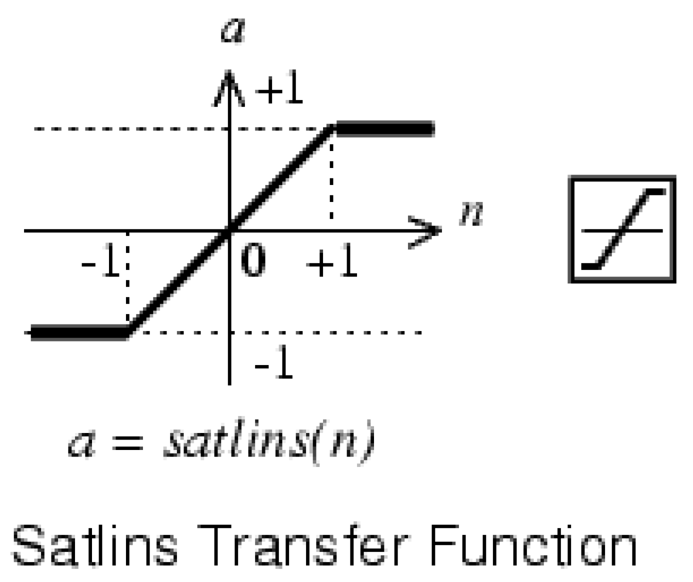
Finally, the transfer function used for all topologies was the symmetric saturated linear function as represented in Figure 9; the function output was linear in the region, while it assumed constant values outside the interval ( for and 1 for ).
3. Results
In this section the results of the analysis will be presented per each network configuration as function of the sampling mode, training function and number of neurons.
3.1. Sampling Mode 1
This is the simplest network architecture based on the first sampling mode, having six inputs and a single hidden layer of size 5 or 6 (Figure 10).
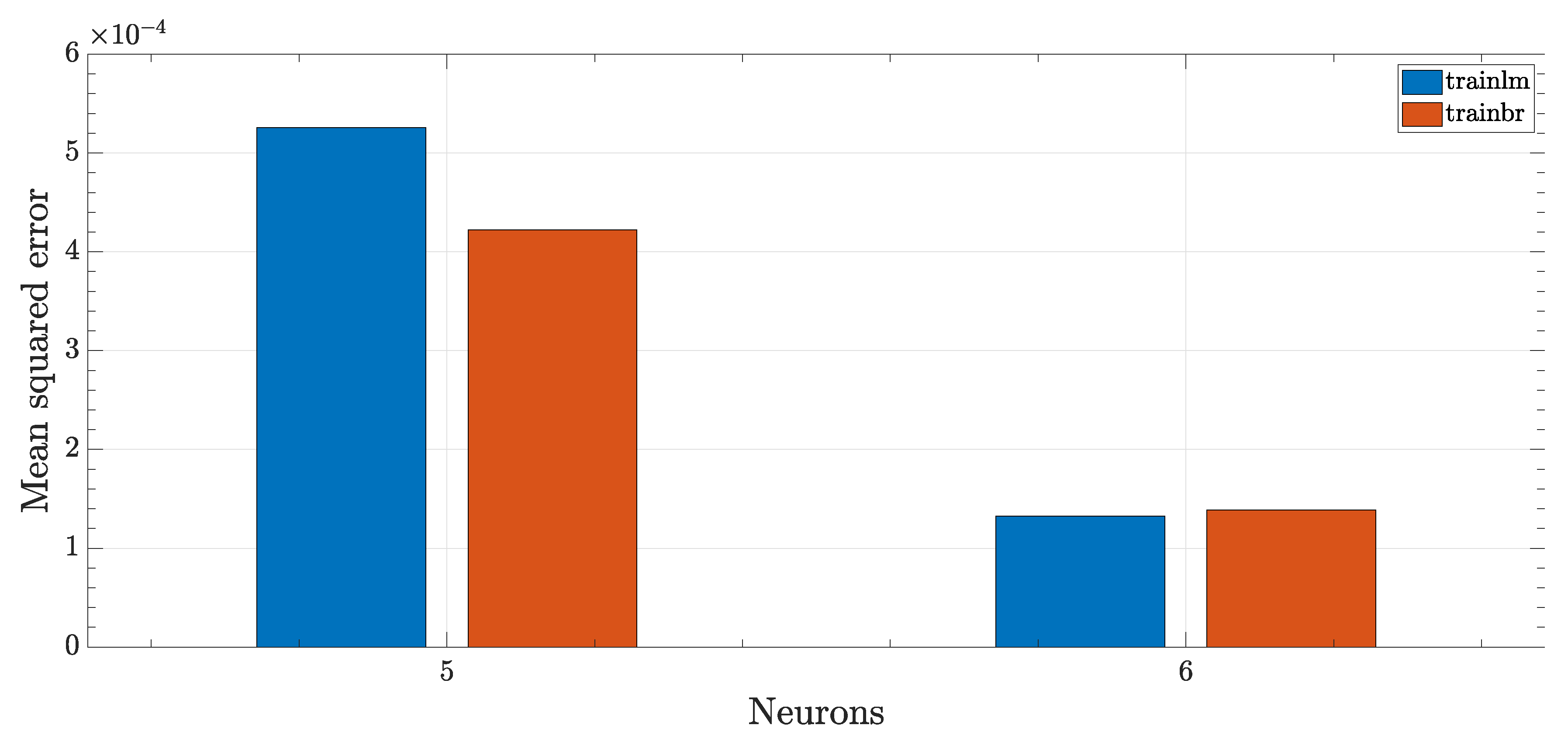
There was a significant boost in performance just by adding a single neuron, even though the performance score was still high (i.e., low accuracy). The Bayesian regression achieved significantly better performance with five neurons, while the difference was negligible considering six neurons.
3.2. Sampling Mode 2
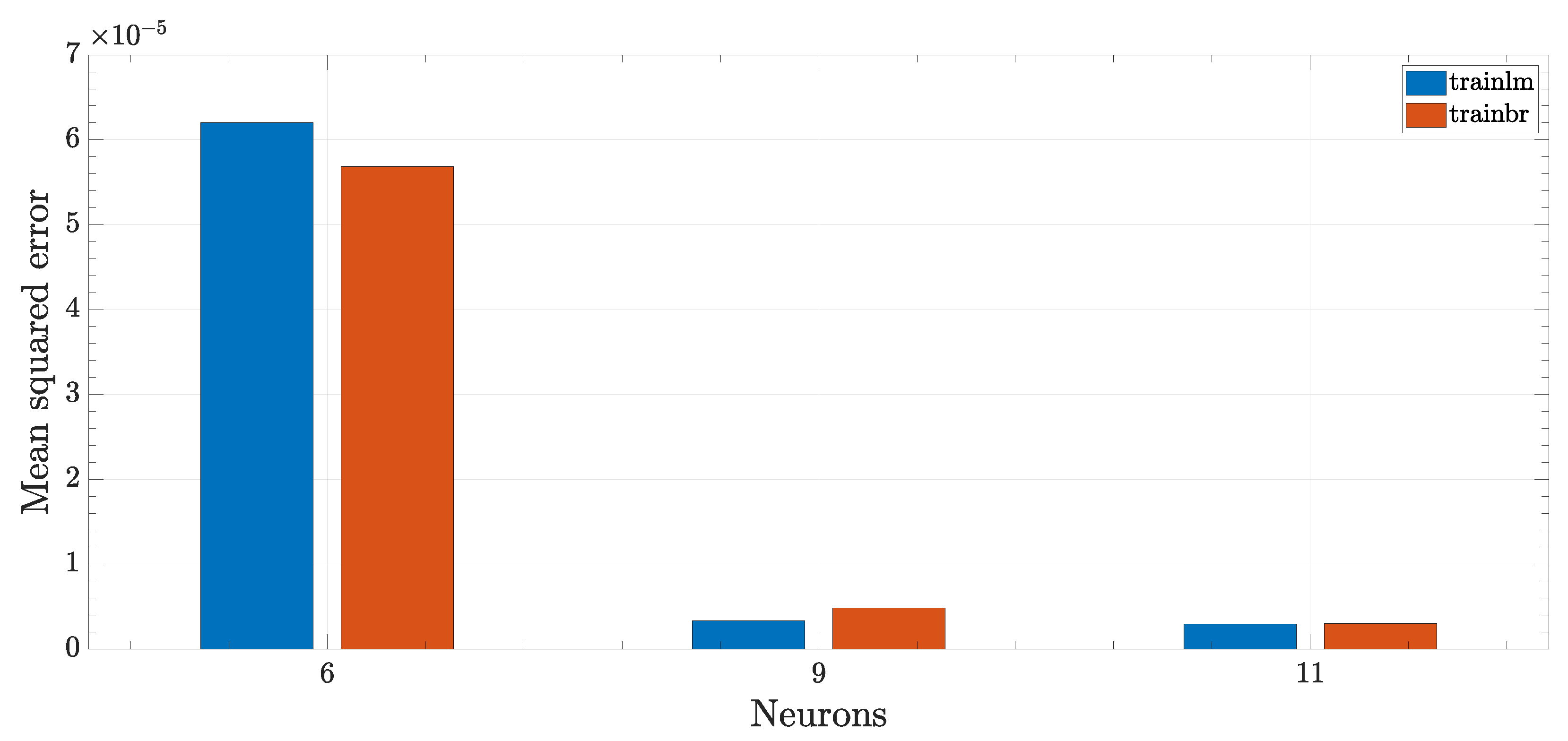
In this case, the number of inputs was increased to two per commutation, that is, 12 in total. The neural networks now had increased complexity but also achieved, globally, a better performance score. For this condition, 6, 9 and 11 neurons networks were considered.
As expected, the performance score (lower is better) decreased with the increase of neurons to value less than in the case of 9 or 11 neurons as visible in Figure 11, thus making much more accurate predictions compared to the first sampling mode.
The difference between the two training algorithms was marginal; considering six neurons, Bayesian regression was superior, while the opposite was true when considering nine neurons. The difference was basically negligible in the 11 neurons case.
3.3. Sampling Mode 3, Single Hidden Layer
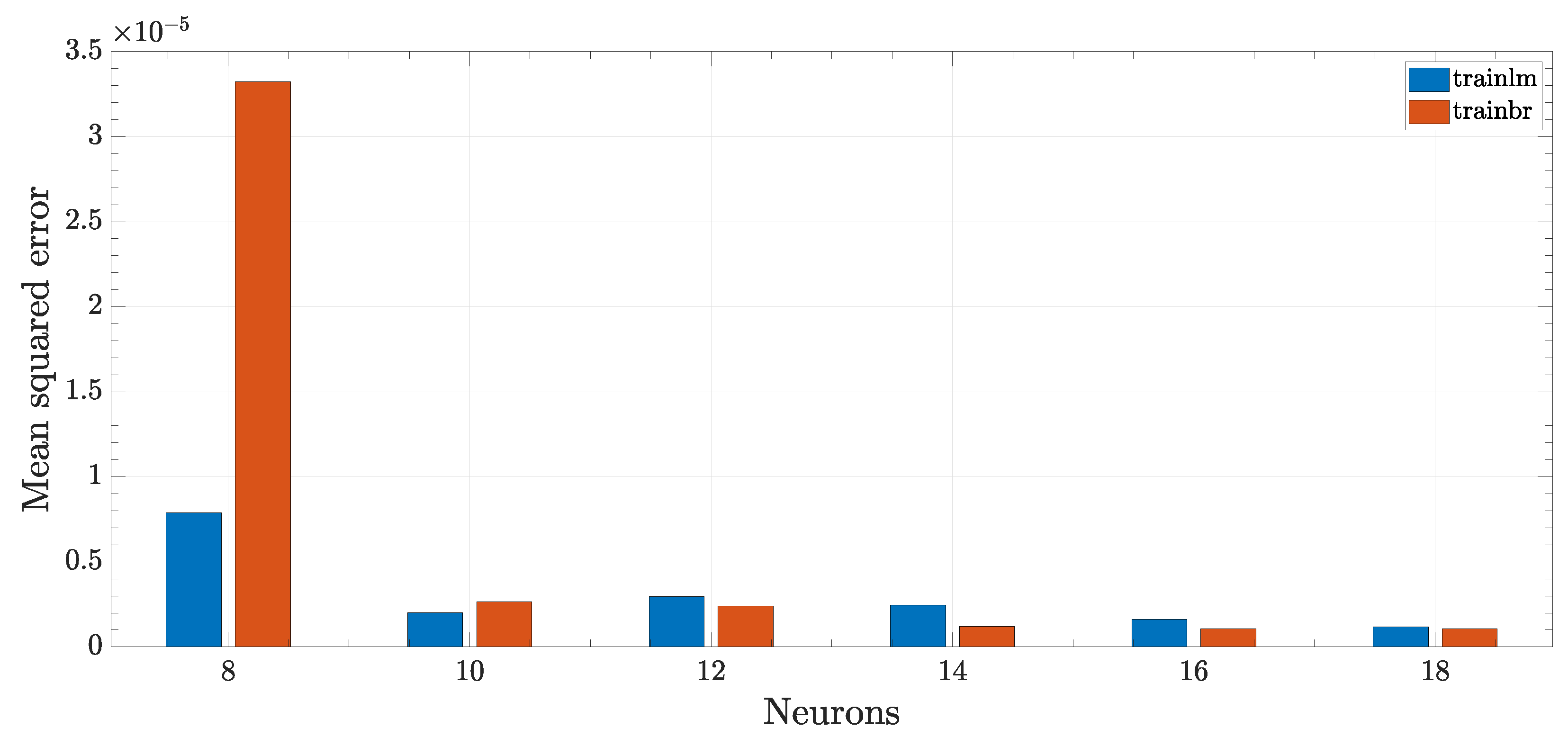
This is the most complex of the configuration analyzed thus far, having now three samples per commutation, thus 18 total inputs. The number of neurons was set to 8, 10, 12, 14 and 16 neurons.
Continuing the established trend, an increase in neuron numbers implies a decrease in performance score, meaning better and more accurate predictions. In this case, the best score achieved was almost as close as the target score, , as visible in Figure 12. In contrast to the previous cases, the Levenberg–Marquardt algorithm performed better with fewer neurons, while the contrary was true for higher complexity networks.
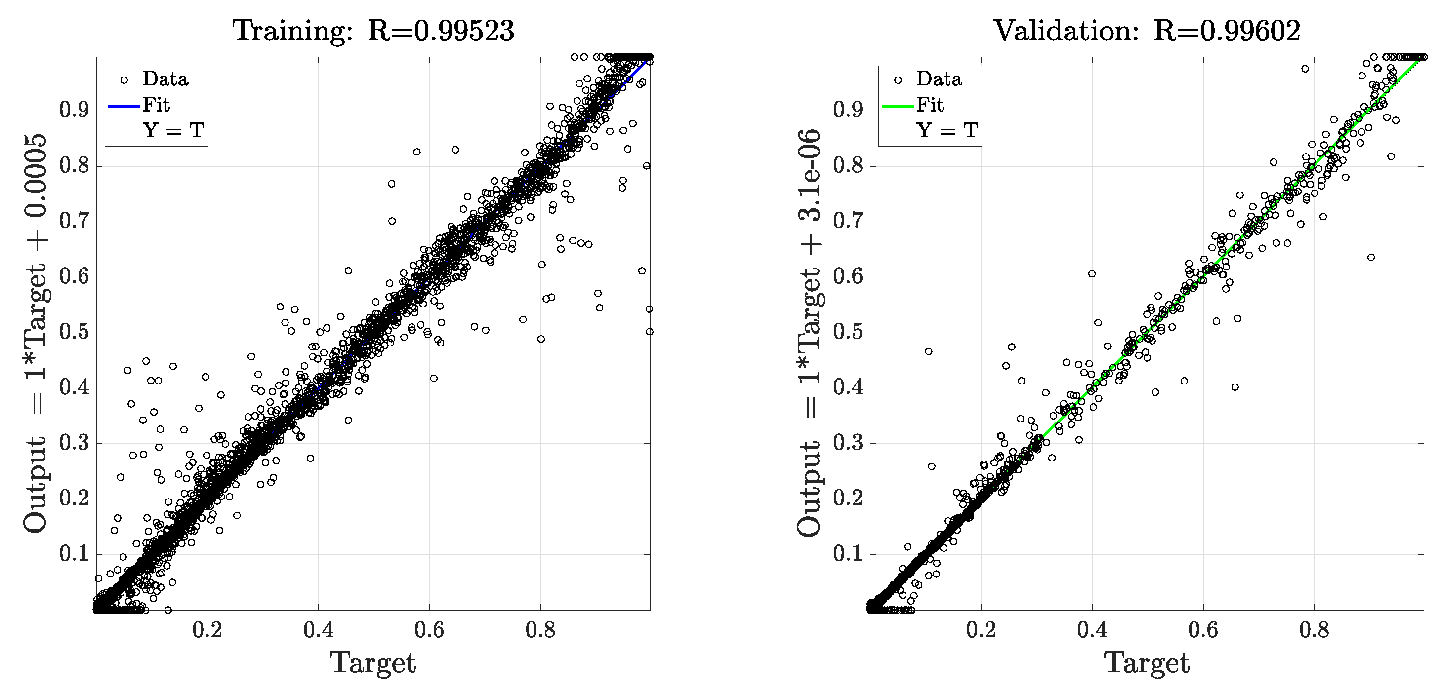
In Figure 13, correlation between targets (i.e., expected outputs) and actual network outputs for sampling mode 3, 18 neurons and trainlm algorithm was reported. It has to be noted that the relatively high number of outliers in both scatter plot can be traced down to an artifact of the representation of eccentricity and relative phase in polar coordinates. As highlighted in Section 2.5, the rotor eccentricity fault was represented in polar coordinates by two fault parameters, encoding the amplitude and phase of eccentricity respectively. As polar coordinates had a singularity in the origin, the phase could not be defined when amplitude was null; additionally, if amplitude was small, the phase was ill-conditioned and large errors in fault detection would appear. However, this behavior was considered acceptable since the information about phase of eccentricity was not relevant for very small fault amplitudes. In any case, the network coefficient of determination () was for the training dataset, for the validation dataset, for the testing datasets and for the complete dataset.
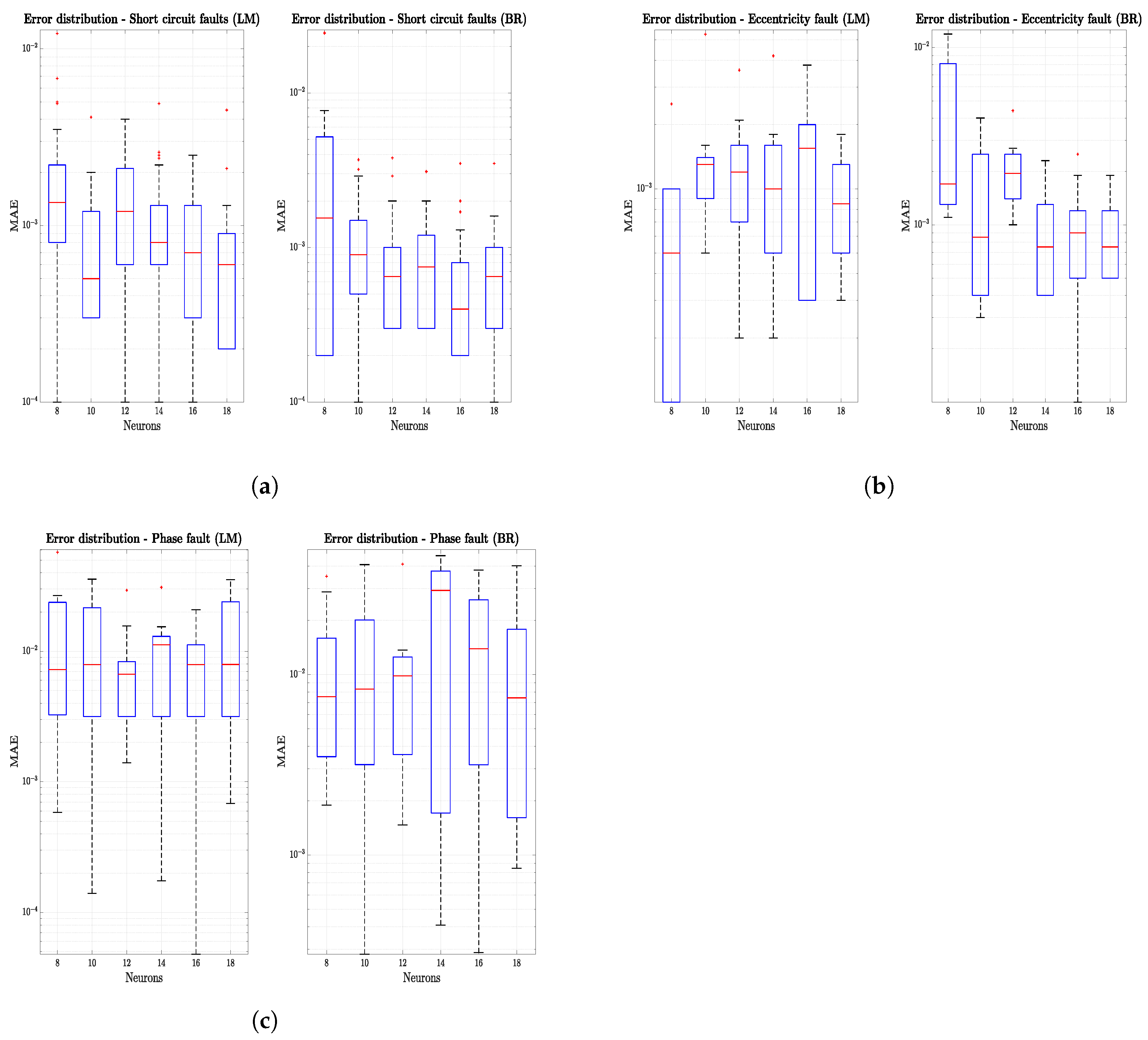
In Figure 14, mean absolute error (MAE) boxplots have been reported for the case of single hidden layer, three input networks using a new custom verification set made of 10 different fault vectors. The general trend was a reduction of the MAE as the number of neurons increased, even though values dispersion did not seem to be affected by the increase in network complexity; this was particularly visible in regards to the phase fault (Figure 14c). Furthermore, no marked difference was observable switching training algorithm from simple Levenberg–Marquardt backpropagation to Bayesian regularization. Anyway, the mean network errors were in the order of , thus generally granting relatively accurate predictions.
3.4. Sampling Mode 3, Double Hidden Layer
This configuration was different from the other one analyzed since it was a double-layer perceptron, having two hidden layers in feedforward configuration.
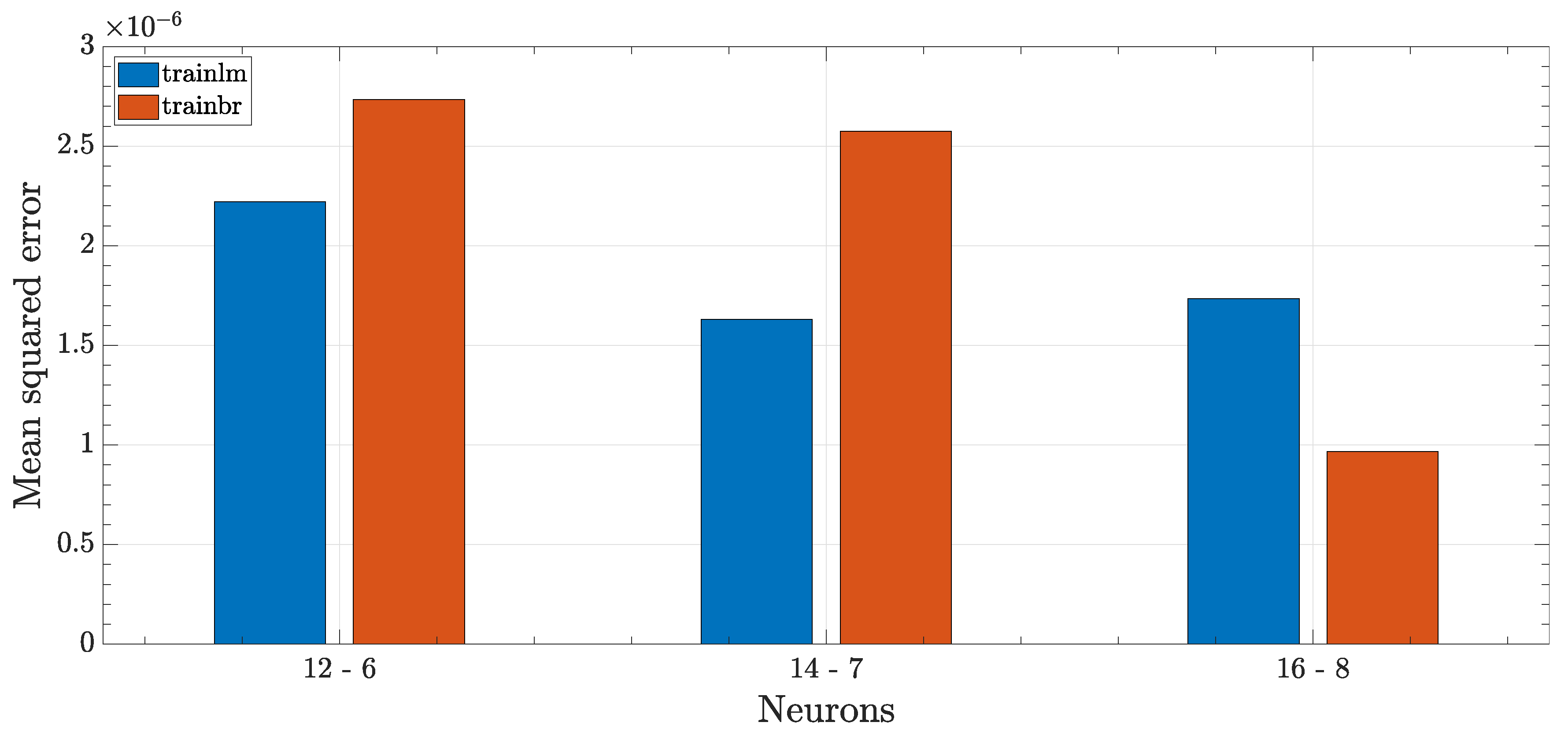
The achieved score was not always better compared to the previous analysis; this implies that an increase in the number of layers was not always associated with an increase in network performance. It has to be noted that the increased complexity of the network, both in terms of neurons and connection increase, resulted in much longer training time, about a three-fold increase when compared to the most complex single layer configuration.
The only configuration capable of achieving a score better than the shallow configuration was the 16-8 network using Bayesian regularization algorithm for training, as visible in Figure 15. In this case, the performance score was less than the set , thus achieving the best score of all the considered configurations.
4. Discussion
In this work, the application of artificial neural networks for prognostic purposes of electromechanical actuators for aerospace applications has been investigated, leveraging a detailed MATLAB Simulink model. The work focused only on particular motor progressive faults, i.e., partial electrical short-circuit and static eccentricity faults.
The process used to evaluate the performance of ANNs has then been described and can be summarized as such: initially, an algorithm generating a vector of faults has been used to create a matrix describing 3000 faults combination between arbitrarily chosen thresholds.
After that, every faults vector has been fed to the Simulink model in order to simulate the real system and important variables such as currents, voltages, mechanical position and angular speed have been logged.
These data have then been used to reconstruct the counter electromotive force coefficient in function of the angular position of the motor. The reconstructed back-EMF has then been sampled using an algorithm to provide data inputs for various ANNs architectures.
Different ANNs architecture have been used as prognostic tools, showing very good performance score, even for very basic architectures. Various sampling strategies have been adopted, generally improving the predictive accuracy of the network increasing the number of inputs of the network itself, i.e., using a higher number of samples for each intracommutation period.
The study has proved that ANNs can be effectively used as prognostics tools for aerospace EMAs. The next step would be a parametric analysis in function of the many different variables defining a neural network, e.g., network architecture, performance function, training function, etc. and an experimental campaign to evaluate the sensitivity to uncertainties in the training model.
After such analysis, a development in lower level language, e.g., C++ can be used to speed up the computation and possibly to allow a field testing campaign in order to evaluate the real-world behavior and performance and the possible implementation on On-Board Computers (OBCs) in prevision of a full-scale, commercial implementation.
Author Contributions
Conceptualization, P.C.B. and M.D.L.D.V.; methodology, P.C.B. and G.Q.; software, M.D.L.D.V., P.C.B. and G.Q.; validation, G.Q. and P.C.B.; formal analysis, G.Q.; investigation, G.Q. and P.C.B.; resources, G.Q.; data curation, G.Q.; writing—original draft preparation, G.Q.; writing—review and editing, P.C.B., M.D.L.D.V. and P.M.; visualization, G.Q.; supervision, M.D.L.D.V. and P.M.; project administration, P.M.; funding acquisition, P.M. All authors have read and agreed to the published version of the manuscript.
Funding
This research received no external funding.
Conflicts of Interest
The authors declare no conflict of interest.
References
- Wheeler, P.; Bozhko, S. The more electric aircraft: Technology and challenges. IEEE Electrif. Mag. 2014, 2, 6–12. [Google Scholar] [CrossRef]
- Van de Bossche, D. More Electric Control Surface Actuation, a Standard for the Next Generation of Transport Aircraft; Control 2004; University of Bath: Bath, UK, 2004; pp. 1–7. [Google Scholar]
- Byington, C.S.; Watson, M.; Edwards, D.; Stoelting, P. A model-based approach to prognostics and health management for flight control actuators. IEEE Aerosp. Conf. Proc. 2004, 6, 3551–3562. [Google Scholar] [CrossRef]
- Hussain, Y.M.; Burrow, S.G.; Henson, L.; Keogh, P. A review of techniques to mitigate jamming in electromechanical actuators for safety critical applications. Int. J. Progn. Health Manag. 2018, 9, 1–11. [Google Scholar]
- Vachtsevanos, G.; Lewis, F.; Roemer, M.; Hess, A.; Wu, B. Intelligent Fault Diagnosis and Prognosis for Engineering Systems; Wiley Hoboken: Hoboken, NJ, USA, 2006. [Google Scholar]
- Liu, J.; Wang, W.; Golnaraghi, F. A multi-step predictor with a variable input pattern for system state forecasting. Mech. Syst. Signal Process. 2009. [Google Scholar] [CrossRef]
- Stetco, A.; Dinmohammadi, F.; Zhao, X.; Robu, V.; Flynn, D.; Barnes, M.; Keane, J.; Nenadic, G. Machine learning methods for wind turbine condition monitoring: A review. Renew. Energy 2019, 133, 620–635. [Google Scholar] [CrossRef]
- Yu, W.K.; Harris, T.A. A new stress-based fatigue life model for ball bearings. Tribol. Trans. 2001. [Google Scholar] [CrossRef]
- Paris, P.; Erdogan, F. A critical analysis of crack propagation laws. In Journal of Fluids Engineering; ASME: New York, NY, USA, 1963. [Google Scholar] [CrossRef]
- Liu, J.; Wang, W.; Ma, F.; Yang, Y.B.; Yang, C.S. A data-model-fusion prognostic framework for dynamic system state forecasting. Eng. Appl. Artif. Intell. 2012, 25, 814–823. [Google Scholar] [CrossRef] [Green Version]
- Liao, L.; Kottig, F. Review of Hybrid Prognostics Approaches for Remaining Useful Life Prediction of Engineered Systems, and an Application to Battery Life Prediction. IEEE Trans. Reliab. 2014, 63, 191–207. [Google Scholar] [CrossRef]
- Mazidi, P.; Bertling Tjernberg, L.; Sanz Bobi, M.A. Wind turbine prognostics and maintenance management based on a hybrid approach of neural networks and a proportional hazards model. Proc. Inst. Mech. Eng. 2017, 231, 121–129. [Google Scholar] [CrossRef]
- Zhang, H.; Kang, R.; Pecht, M. A hybrid prognostics and health management approach for condition-based maintenance. In Proceedings of the 2009 IEEE International Conference on Industrial Engineering and Engineering Management, Hong Kong, China, 8–11 December 2009; pp. 1165–1169. [Google Scholar] [CrossRef]
- Leboeuf, N.; Boileau, T.; Nahid-Mobarakeh, B.; Clerc, G.; Meibody-Tabar, F. Real-Time Detection of Interturn Faults in PM Drives Using Back-EMF Estimation and Residual Analysis. IEEE Trans. Ind. Appl. 2011, 47, 2402–2412. [Google Scholar] [CrossRef]
- Dalla Vedova, M.D.; Berri, P.C. Optimization techniques for prognostics of on-board electromechanical servomechanisms affected by progressive faults. Int. Rev. Aerosp. Eng. 2019, 12, 160–170. [Google Scholar] [CrossRef]
- Dalla Vedova, M.D.; Berri, P.C.; Re, S. A Comparison of Bio-Inspired Meta-Heuristic Algorithms for Aircraft Actuator Prognostics. In Proceedings of the 29th European Safety and Reliability Conference, Hannover, Germany, 22–26 September 2019; pp. 1064–1071. [Google Scholar] [CrossRef] [Green Version]
- Jin, W.; Chen, Y.; Lee, J. Methodology for Ball Screw Component Health Assessment and Failure Analysis. In Volume 2: Systems; Micro and Nano Technologies; Sustainable Manufacturing; American Society of Mechanical Engineers: New York, NY, USA, 2013. [Google Scholar] [CrossRef]
- Skirtich, T.; Siegel, D.; Lee, J.; Pavel, R. A systematic health monitoring and fault identification methodology for machine tool feed axis. In Proceedings of the Technical Program for MFPT: The Applied Systems Health Management Conference 2011: Enabling Sustainable Systems, Virginia Beach, VA, USA, 10–12 May 2011. [Google Scholar]
- Li, X.; Ding, Q.; Sun, J.Q. Remaining useful life estimation in prognostics using deep convolution neural networks. Reliab. Eng. Syst. Saf. 2018, 172, 1–11. [Google Scholar] [CrossRef] [Green Version]
- Listou Ellefsen, A.; Bjørlykhaug, E.; Æsøy, V.; Ushakov, S.; Zhang, H. Remaining useful life predictions for turbofan engine degradation using semi-supervised deep architecture. Reliab. Eng. Syst. Saf. 2019, 183, 240–251. [Google Scholar] [CrossRef]
- Guo, L.; Li, N.; Jia, F.; Lei, Y.; Lin, J. A recurrent neural network based health indicator for remaining useful life prediction of bearings. Neurocomputing 2017, 240, 98–109. [Google Scholar] [CrossRef]
- Zhang, J.; Wang, P.; Yan, R.; Gao, R.X. Long short-term memory for machine remaining life prediction. J. Manuf. Syst. 2018, 48, 78–86. [Google Scholar] [CrossRef]
- Xia, M.; Zheng, X.; Imran, M.; Shoaib, M. Data-driven prognosis method using hybrid deep recurrent neural network. App. Soft Comput. 2020, 93, 106351. [Google Scholar] [CrossRef]
- Elsheikh, A.; Yacout, S.; Ouali, M.S. Bidirectional handshaking LSTM for remaining useful life prediction. Neurocomputing 2019, 323, 148–156. [Google Scholar] [CrossRef]
- Al-Dulaimi, A.; Zabihi, S.; Asif, A.; Mohammadi, A. A multimodal and hybrid deep neural network model for Remaining Useful Life estimation. Comput. Ind. 2019, 108, 186–196. [Google Scholar] [CrossRef]
- Baptista, M.; Henriques, E.P.; de Medeiros, I.P.; Malere, J.P.; Nascimento, C.L.; Prendinger, H. Remaining useful life estimation in aeronautics: Combining data-driven and Kalman filtering. Reliab. Eng. Syst. Saf. 2019, 184, 228–239. [Google Scholar] [CrossRef]
- Liu, J.; Zhang, M.; Zuo, H.; Xie, J. Remaining useful life prognostics for aeroengine based on superstatistics and information fusion. Chin. J. Aeronaut. 2014, 27, 1086–1096. [Google Scholar] [CrossRef] [Green Version]
- Li, Q.; Gao, Z.; Tang, D.; Li, B. Remaining useful life estimation for deteriorating systems with time-varying operational conditions and condition-specific failure zones. Chin. J. Aeronaut. 2016, 29, 662–674. [Google Scholar] [CrossRef] [Green Version]
- Sun, J.; Wang, F.; Ning, S. Aircraft air conditioning system health state estimation and prediction for predictive maintenance. Chin. J. Aeronaut. 2019. [Google Scholar] [CrossRef]
- Baraldi, P.; Mangili, F.; Zio, E. Investigation of uncertainty treatment capability of model-based and data-driven prognostic methods using simulated data. Reliab. Eng. Syst. Saf. 2013, 112, 94–108. [Google Scholar] [CrossRef] [Green Version]
- Djeziri, M.A.; Benmoussa, S.; Benbouzid, M.E. Data-driven approach augmented in simulation for robust fault prognosis. Eng. Appl. Artif. Intell. 2019, 86, 154–164. [Google Scholar] [CrossRef]
- Berri, P.C.; Dalla Vedova, M.D.L.; Maggiore, P. A Lumped Parameter High Fidelity EMA Model for Model-Based Prognostics. In Proceedings of the 29th European Safety and Reliability Conference (ESREL), Hannover, Germany, 22–26 September 2019; Research Publishing Services: Singapore, 2019; pp. 1086–1093. [Google Scholar] [CrossRef]
- Quattrocchi, G.; Berri, P.C.; Dalla Vedova, M.D.L.; Maggiore, P. Back-EMF reconstruction for electromechanical actuators in presence of faults. In Proceedings of the 30th European Safety and Reliability Conference and the 15th Probabilistic Safety Assessment and Management Conference, Venice, Italy, 21–26 June 2020. [Google Scholar]
- Stevens, B.L.; Lewis, F.L.; Johnson, E.N. Aircraft Control and Simulation: Dynamics, Controls Design, and Autonomous Systems; John Wiley & Sons: Hoboken, NJ, USA, 2015. [Google Scholar] [CrossRef]
- Marquardt, D.W. An Algorithm for Least-Squares Estimation of Nonlinear Parameters. J. Soc. Ind. Appl. Math. 1963. [Google Scholar] [CrossRef]
- Hagan, M.T.; Menhaj, M.B. Training Feedforward Networks with the Marquardt Algorithm. IEEE Trans. Neural Netw. 1994. [Google Scholar] [CrossRef] [PubMed]
- Foresee, F.D.; Hagan, M.T.; Dan Foresee, F.; Hagan, M.T. Gauss-Newton approximation to bayesian learning. In Proceedings of the IEEE International Conference on Neural Networks, Houston, TX, USA, 12 June 1997. [Google Scholar] [CrossRef]
Figure 1.
Prognostics algorithm schematization.

Figure 2.
Model overview [33].
Figure 2.
Model overview [33].

Figure 3.
Trapezoidal EMA subsystem [33].
Figure 3.
Trapezoidal EMA subsystem [33].

Figure 4.
F16 longitudinal dynamics model [34].
Figure 4.
F16 longitudinal dynamics model [34].

Figure 5.
Normalized reconstructed back electromotive force (back-EMF) coefficient in nominal and faulty condition.
Figure 5.
Normalized reconstructed back electromotive force (back-EMF) coefficient in nominal and faulty condition.

Figure 6.
Variation of m for two different intra-commutations periods considering 5 randomly seeded back-EMF coefficient curves.
Figure 6.
Variation of m for two different intra-commutations periods considering 5 randomly seeded back-EMF coefficient curves.

Figure 7.
Discretization of five randomly seeded reconstructed back-EMF coefficient curves.

Figure 8.
Example of single hidden layer perceptron.

Figure 9.
Saturated linear symmetric transfer function.

Figure 10.
Single hidden layer networks performance as function of neurons and training function, sampling mode 1.
Figure 10.
Single hidden layer networks performance as function of neurons and training function, sampling mode 1.

Figure 11.
Single hidden layer networks performance as function of neurons and training function, sampling mode 2.
Figure 11.
Single hidden layer networks performance as function of neurons and training function, sampling mode 2.

Figure 12.
Single hidden layer networks performance as function of neurons and training function, sampling mode 3.
Figure 12.
Single hidden layer networks performance as function of neurons and training function, sampling mode 3.

Figure 13.
Correlation between targets (i.e., expected outputs) and actual outputs of the network for sampling mode 3, 18 neurons and trainlm algorithm, for training and validation datasets.
Figure 13.
Correlation between targets (i.e., expected outputs) and actual outputs of the network for sampling mode 3, 18 neurons and trainlm algorithm, for training and validation datasets.

Figure 14.
Distribution of the mean absolute error (MAE) on the identification of the considered
fault modes, for increasing number of neurons in the layer. Errors were determined for a custom
identification set, randomly sampled in the acceptable range defined by Equations (2) and (3). (a) Short circuits. (b) Eccentricity. (c) Phase.

Figure 15.
Double hidden layer networks performance as function of neurons and training function, sampling mode 3.
Figure 15.
Double hidden layer networks performance as function of neurons and training function, sampling mode 3.

© 2020 by the authors. Licensee MDPI, Basel, Switzerland. This article is an open access article distributed under the terms and conditions of the Creative Commons Attribution (CC BY) license (http://creativecommons.org/licenses/by/4.0/).
Share and Cite
MDPI and ACS Style
Quattrocchi, G.; Berri, P.C.; Dalla Vedova, M.D.L.; Maggiore, P. Innovative Actuator Fault Identification Based on Back Electromotive Force Reconstruction. Actuators 2020, 9, 50. https://0-doi-org.brum.beds.ac.uk/10.3390/act9030050
AMA Style
Quattrocchi G, Berri PC, Dalla Vedova MDL, Maggiore P. Innovative Actuator Fault Identification Based on Back Electromotive Force Reconstruction. Actuators. 2020; 9(3):50. https://0-doi-org.brum.beds.ac.uk/10.3390/act9030050
Chicago/Turabian StyleQuattrocchi, Gaetano, Pier C. Berri, Matteo D. L. Dalla Vedova, and Paolo Maggiore. 2020. "Innovative Actuator Fault Identification Based on Back Electromotive Force Reconstruction" Actuators 9, no. 3: 50. https://0-doi-org.brum.beds.ac.uk/10.3390/act9030050
Note that from the first issue of 2016, this journal uses article numbers instead of page numbers. See further details here.