Article

Analytical Analysis of Magnetic Levitation Systems with Harmonic Voltage Input

by
Serguei Maximov
1,†,
Felipe Gonzalez-Montañez
2,†,
Rafael Escarela-Perez
2,*,†,
Juan Carlos Olivares-Galvan
2,† and
Hector Ascencion-Mestiza
1,†
1
Posgrado en Eléctrica, Tecnológico Nacional de México, Instituto Tecnológico de Morelia, Morelia C.P. 58120, Mexico
2
Departamento de Enérgia, Universidad Autónoma Metropolitana Azcapotzalco, Ciudad de México C.P. 02200, Mexico
*
Author to whom correspondence should be addressed.
These authors contributed equally to this work.
Submission received: 30 July 2020 / Revised: 30 August 2020 / Accepted: 9 September 2020 / Published: 11 September 2020
(This article belongs to the Special Issue Electromagnetic Levitation Actuators)

Abstract

:
In this paper, a new analytical method using Lagrange equations for the analysis of magnetic levitation (MagLev) systems is proposed, using Thomson’s jumping ring experiment. The method establishes the dependence of the primary and induced currents, and also the equilibrium height of the levitating object on the input voltage through the mutual inductance of the system. The mutual inductance is calculated in two ways: (i) by employing analytical formula; (ii) through an improved semi-empirical formula based on both measurements and analytical results. The obtained MagLev model was analyzed both analytically and numerically. Analytical solutions to the resulting equations were found for the case of a dynamic equilibrium. The numerical results obtained for the dynamical model under transient operation show a close correspondence with the experimental results. The good precision of the analytical and numerical results demonstrates that the developed method can be effectively implemented.

1. Introduction

The principles of magnetic levitation (MagLev) are used in many important applications, such as actuators, power interrupters for eliminating electric arcs, electromagnetic shock absorbers in electrical vehicles, hybrid suspension systems with active control, levitation of superconductor materials, sensors and electromagnetic mass drivers [1]. One of the perspective usages of the MagLev systems in the near future is related to electromagnetic suspension systems and damping shock absorbers. Automobiles and trucks have shock absorbers with similar geometry to that of Thomson’s ring system. These systems are used to damper vibrations generated by imperfections of road surfaces [2,3,4,5].
Thus, it is an important challenge to be able mathematically and numerically model, analyze, control and design MagLev devices similar to Thomson’s ring system. There are also highly accurate density measurements and density-based detection methods applied to MagLev systems with similar geometries. In [6,7,8], an experimental study of a single-ring MagLev system was presented, opening up a wide operational space and enabling object manipulation and density-based measurements.
In the literature, there are works focused on the numerical analysis of MagLev systems similar to that of Thomson’s ring. Vilchis et al. [9] presented factors that affect 2D finite element method (FEM) transient simulation accuracy for an axisymmetric model of a Thomson-coil actuator. Yannan Zhou et al. [10] numerically studied a Thomson-coil actuator applied in a circuit breaker in a high-voltage direct current system. Tezuka et al. [11] proposed a novel magnetically-levitating motor, able to control five degrees of freedom. In all these systems, analytical or hybrid solutions can be implemented, resulting in accurate and low-demanding computational models.
Dynamic models (DM) of the MagLev systems have been previously developed. TJ-Teo et al. [12] presented a new electromagnetic actuator which has two degrees of freedom (linear and rotary motions). Consequently, the developed MagLev system presents two mutual inductances as functions of linear and rotatory positions. Additionally, Nagai et al. [13] realized a compact actuator system by a sensor-free approach. They presented the circuit equations for the solenoid, where the mutual inductance was approximated as a second-order polynomial function.
Here, we present a new and rigorous analytical solution to the dynamic equations of the MagLev systems, wherein a mutual inductance, which is the key parameter of electromagnetic force, is calculated analytically. This way, we obtain a method that retains the simplicity of lumped-parameter models plus the accuracy of analytical methods within a field modeling context. Our approach was validated using experimental test results obtained from a Thomson’s jumping ring experiment.

2. Model

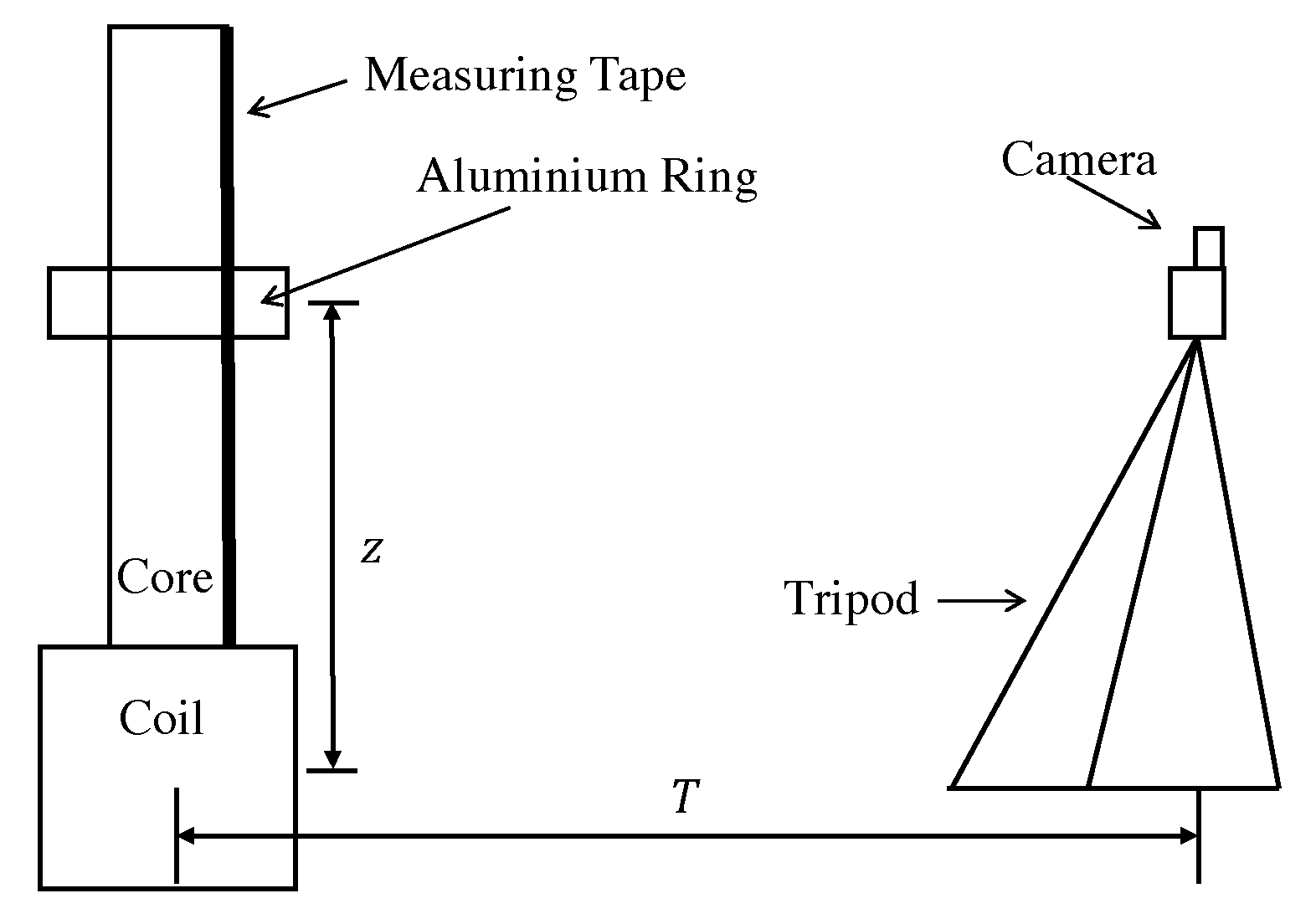
In this work, a system known as the Thomson’s jumping ring is studied, where an aluminum ring is used as a levitating object. The experimental setup is shown in Figure 1. The system is composed of a primary copper coil of 1140 turns, and an aluminum ring that moves freely up and down along a laminated ferromagnetic core.
The equivalent circuit depicted in Figure 2 models this MagLev system.
The governing differential equations that govern the dynamics of the circuit represented in Figure 2 can be obtained from the Lagrangian
L = l 1 i 1 2 2 + l 2 i 2 2 2 + M i 1 i 2 + m z ˙ 2 2 kinetic energy m g z potential energy ,
where z is the ring height, and i 1 and i 2 are the electric currents in the primary coil and aluminum ring, respectively. The parameters l 1 and l 2 are the primary and secondary circuits’ inductances; M is the mutual inductance between the coil and ring; and m and g are the aluminum ring mass and gravitational constant, respectively. Notice that the mutual inductance M ( z ) is a function of the distance z between the coil and ring [14]. Thus, the Lagrange equations are as follows:
d d t L i 1 L q 1 = V ( t ) R 1 i 1 ,
d d t L i 2 L q 2 = R 2 i 2 ,
d d t L z ˙ L z = β z ˙ ,
where R 1 and R 2 are the coil and ring resistances; q 1 and q 2 are the coil and ring electric charges, respectively; and β is the friction coefficient. The right-hand side terms of the Lagrange equations are generalized forces, which are considered as independent terms, associated with the generalized coordinate. Substitution of the Lagrangian (1) into Lagrange equations results in the following system of differential equations (see also [15,16]):
l 1 d i 1 d t = V ( t ) R 1 i 1 d ( M ( z ) i 2 ) d t
l 2 d i 2 d t = R 2 i 2 d ( M ( z ) i 1 ) d t ,
m z ¨ = i 1 i 2 d M ( z ) d z β z ˙ m g .

3. Formula for the Mutual Inductance

Mutual inductance between a coil and aluminum ring is a function of the system geometry and the magnetic medium properties between two coils. It can be calculated in two ways: numerically (using FEM) or analytically. In this section, the linear mutual inductance is analytically calculated based on the results of [17], where an infinite isotropic core is considered. According to [17], the mutual inductance can be divided into two parts:
M = M air + M core ,
where M air is the mutual inductance in air, i.e., in the absence of the core, and M core is the contribution of the ferromagnetic core to the whole inductance. The first part of the mutual inductance can be represented in the form (see [17]):
M air = μ 0 N a w a h a w b h b a a + h a d A b b + h b d B w a 0 d z a z z + w b d z b × 2 A B f 1 f 2 2 K ( f ) E ( f ) ,
where
f = 4 r a r b z b z a 2 + r a + r b 2
is a dimensionless parameter; K ( f ) and E ( f ) are complete elliptic integrals of the first and second kind, respectively [18]. Here, ( r a , z a ) and ( r b , z b ) are pairs of cylindrical coordinates inside the coil and ring (subindices a and b correspond to the coil and aluminum ring, respectively). Namely, r a and r b are radii-vectors and z a and z b positions on the core. Integration with respect to these variables signifies that the whole volume of the coil and ring is involved in the calculation of the mutual inductance between them. Parameters w a and w b are the coil and ring widths; h a and h b are their heights; and a and b are their internal radii (see Figure 3). N a is the number of turns in the coil. The mutual inductance caused by the core is as follows:
M core = 2 μ 0 N a w a h a w b h b 0 d k k 2 × cos k ( z + w b ) + cos k ( z + w a ) cos ( k z ) cos k ( z + w a + w b ) × π 2 k ( a + h a ) [ K 1 k ( a + h a ) L 0 k ( a + h a ) + K 0 k ( a + h a ) L 1 k ( a + h a ) ] a K 1 ( k a ) L 0 ( k a ) + K 0 ( k a ) L 1 ( k a ) π 2 k ( b + h b ) [ K 1 k ( b + h b ) L 0 k ( b + h b ) + K 0 k ( b + h b ) L 1 k ( b + h b ) ] b K 1 ( k b ) L 0 ( k b ) + K 0 ( k b ) L 1 ( k b ) × μ r k I 1 ( β R ) I 0 ( k R ) β I 0 ( β R ) I 1 ( k R ) μ r k I 1 ( β R ) K 0 ( k R ) β I 0 ( β R ) K 1 ( k R ) ,
where β = k 2 + j ω μ σ , μ = μ 0 μ r is the absolute permeability of the core material, μ r is its relative permeability and σ is core conductance.
The total mutual inductance is a function of the ring position z; i.e., M = M ( z ) . Equations (9) and (11) are too complicated to be implemented in the dynamical analysis of the MagLev system. Equations (9) and (11), and FEM calculations, are too complicated and time-consuming to be implemented in the dynamical analysis of the MagLev system, especially in real-time calculations for an electromagnetic suspension system. Therefore, equations (9) and (
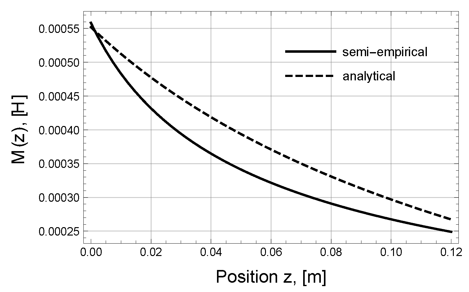
11) must be simplified. In Figure 4, analytical behavior of the total inductance of the ring height is depicted. It can be seen in Figure 4 that the total mutual inductance of the system can be approximated by exponential function as follows:
M ( z ) = α 1 e β 1 z + α 2 e β 2 z ,
where α 1 , α 2 , β 1 and β 2 are some empirical parameters to be obtained by fitting function (12) to the analytical result. The reason for the use of (12), apart from reproducing qualitatively theoretical results (9) and (11), is that it provides a correct asymptotic behavior of the mutual inductance at large distances. A polynomial approximation would diverge at high distances. The numerical values of the parameters involved in (12) can be obtained from (9) and (11) through the widely-used least squares method [19]. As a result, the following values can be obtained: α 1 = 0.000464 H, α 2 = 0.000088 H, β 1 = 4.77562 m−1 and β 2 = 22.74612 m−1. The behavior of the simplified formula for mutual inductance is presented in Figure 4. The precision of the approximation by (12) is such that both curves (the analytical and simplified) are indistinguishable. Another advantage of the approximation (12) is that it can be easily implemented in subsequent analytical calculations.

4. Analytical Solution

In this section, the asymptotic solution of the system of Equations (5)–(7) is found in steady state conditions. The smallness of the mutual inductance (see parameters α 1 and α 2 ) makes possible the implementation of the perturbation theory (PT). This fact is emphasized using a small dimensionless parameter ε 1 , which is included in the set of Equations (5)–(7) as follows:
l 1 d i 1 d t + R 1 i 1 = V ( t ) ε M d i 2 d t ε i 2 d M d t ,
l 2 d i 2 d t + R 2 i 2 = ε M d i 1 d t ε i 1 d M d t ,
z ¨ = ε i 1 i 2 m d M d z β m z ˙ ε 2 g ,
where the multiplier ε 2 next to the last term on the right-hand side of Equation (15) has been placed in order to provide the existence of a bounded steady state solution to the equation system (13)–(15).
A harmonic input voltage in the primary circuit is assumed:
V ( t ) = 1 2 V e j ω t + V * e j ω t
where V and V * are complex amplitudes ( V * is the complex conjugate of V). Notice that Equation (16) gives a cosine-form input voltage. Indeed, complex amplitude V can be represented in the form: V = V e j ϕ , where ϕ is the phase. Then, V * = V e j ϕ . Substitution of these expressions into Equation (16) yields: V ( t ) = V cos ( ω t + ϕ ) . Although the input voltage is of the cosine form, higher harmonics in the currents i 1 ( t ) and i 2 ( t ) and the height z ( t ) appear due to the fact that Equations (13)–(15) are nonlinear. According to PT, they can be expanded into a power series with respect to the small parameter ε as follows:
i k ( t ) = i k , 0 ( t ) + ε i k , 1 ( t ) + ε 2 i k , 2 ( t ) + O ε 3 ,
z ( t ) = z 0 ( t ) + ε z 1 ( t ) + ε 2 z 2 ( t ) + O ε 3 ,
where k = 1 , 2 , and O ε 3 refers to the well-known Landau big- O notation. i k , n ( t ) (where k = 1 , 2 ) and z n ( t ) are the nth order PT contributions to the primary and secondary currents and the ring coordinate (height), respectively.
The substitution of the expansions (17) and (18) into the system (13)–(15) leads to an infinite chain of equations. According to PT, it can be truncated at a certain term. As a result, the zero order of PT yields:
l 1 d i 1 , 0 d t + R 1 i 1 , 0 = V ( t ) ,
l 2 d i 2 , 0 d t + R 2 i 2 , 0 = 0 ,
z ¨ 0 = β m z ˙ 0 .
The general solution to Equation (21) is
z 0 = C 1 + C 2 e β t / m ,
where C 1 and C 2 are constants. In can be seen in (22) that the unique steady state solution to Equation (21) is
z 0 = const .
This solution represents the equilibrium position of the ring. The explicit form of z 0 will be found below for higher orders of PT.
After taking into account the solution (23), the system of Equations (13)–(15) in the first order of PT becomes:
l 1 d i 1 , 1 d t + R 1 i 1 , 1 = M ( z 0 ) d i 2 , 0 d t ,
l 2 d i 2 , 1 d t + R 2 i 2 , 1 = M ( z 0 ) d i 1 , 0 d t ,
z ¨ 1 = i 1 , 0 i 2 , 0 m M ( z 0 ) β m z ˙ 1 .
Finally, second order of PT leads to:
l 1 d i 1 , 2 d t + R 1 i 1 , 2 = M ( z 0 ) d i 2 , 1 d t M ( z 0 ) z 1 d i 2 , 0 d t M ( z 0 ) z 1 ˙ i 2 , 0 ,
l 2 d i 2 , 2 d t + R 2 i 2 , 2 = M ( z 0 ) d i 1 , 1 d t M ( z 0 ) z 1 d i 1 , 0 d t M ( z 0 ) z ˙ 1 i 1 , 0 ,
z ¨ 2 = 1 m i 1 , 0 i 2 , 0 M ( z 0 ) z 1 + i 1 , 0 i 2 , 1 + i 1 , 1 i 2 , 0 M ( z 0 ) β m z ˙ 2 g .
The input voltage (16), in the dynamic equilibrium state, produces periodic currents i k ( t ) and a periodic coordinate z ( t ) , so that each term of the expansions (17) and (18) can be in turn expanded respectively in Fourier series as follows:
i k , n ( t ) = p = i k , n [ p ] e j p ω t , k = 1 , 2
z n ( t ) = p = z n [ p ] e j p ω t ,
where i k , n [ p ] and z n [ p ] are complex amplitudes. Equations (17) and (18) should be substituted into Equations (19)–(29), and the amplitudes of their respective harmonics should be equated in both parts of each equation. As a result, we will obtain a system of algebraic Equations that connect Fourier coefficients i k , n [ p ] and z n [ p ] with the input voltage amplitude | V | . Substitution of (30) into Equations (19) and (20) yields:
p = j p ω l 1 + R 1 i 1 , 0 [ p ] e j p ω t = 1 2 V e j ω t + V * e j ω t ,
p = j p ω l 2 + R 2 i 2 , 0 [ p ] e j p ω t = 0 .
The solutions to these equations are:
i 1 , 0 [ p ] = 1 2 V δ p , 1 + V * δ p , 1 R 1 + j p ω l 1 ,
i 2 , 0 [ p ] = 0 ,
where δ p , l is the symbol of Kronecker. After substituting these results into (30), the form of the currents in the time domain in the zero order of PT can be obtained:
i 1 , 0 ( t ) = Re V e j ω t R 1 + j ω l 1 ,
i 2 , 0 ( t ) = 0 .
Similarly, first and second orders of PT are calculated as:
i 1 , 1 ( t ) = 0 ,
i 2 , 1 ( t ) = Im ω M ( z 0 ) V e j ω t ( R 1 + j ω l 1 ) ( R 2 + j ω l 2 ) ,
z 1 = const ,
i 1 , 2 ( t ) = Re ω 2 M 2 ( z 0 ) V e j ω t ( R 1 + j ω l 1 ) 2 ( R 2 + j ω l 2 ) ,
i 2 , 2 ( t ) = z 1 Im ω M ( z 0 ) V e j ω t ( R 1 + j ω l 1 ) ( R 2 + j ω l 2 ) .
Substitution of (30) into Equation (29) with solutions (36)–(42) taken into account results in the following equation after some simplifications:
z ¨ 2 = j ω M ( z 0 ) M ( z 0 ) 4 m { V 2 e j 2 ω t ( R 1 + j ω l 1 ) 2 ( R 2 + j ω l 2 ) V * 2 e j 2 ω t ( R 1 j ω l 1 ) 2 ( R 2 j ω l 2 ) 2 j ω l 2 | V | 2 ( R 1 2 + ω 2 l 1 2 ) ( R 2 2 + ω 2 l 2 2 ) } β m z ˙ 2 g
Equation (43) has a solution that linearly increases with time. To avoid this instability, it is necessary to equate the constant part on the right-hand side of (
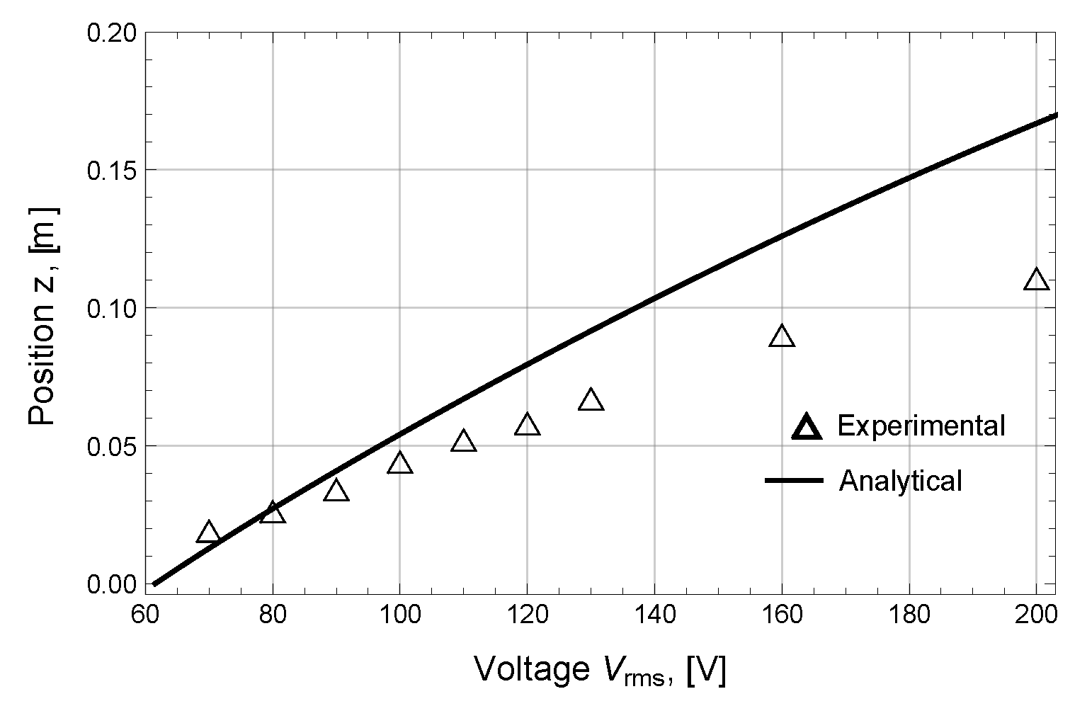
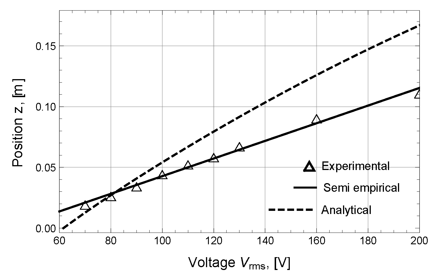
43) to zero. As a result, the following equation can be obtained:
ω 2 l 2 M ( z 0 ) M ( z 0 ) | V | 2 2 m ( R 1 2 + ω 2 l 1 2 ) ( R 2 2 + ω 2 l 2 2 ) g = 0 .
This equation associates the equilibrium height z 0 with the input voltage amplitude | V | . In order to establish the dependence of the ring position on the input voltage amplitude, the simplified formula for mutual inductance (12) should be substituted into Equation (44). Therefore, we come across with the following transcendental equation:
ω 2 l 2 | V | 2 2 m ( R 1 2 + ω 2 l 1 2 ) ( R 2 2 + ω 2 l 2 2 ) α 1 e β 1 z 0 + α 2 e β 2 z 0 × α 1 β 1 e β 1 z 0 + α 2 β 2 e β 2 z 0 = g ,
which can be numerically solved with respect to the ring position.
After taking into account (44), the solution to Equation (43) can be found in the form:
z 2 ( t ) = M ( z 0 ) M ( z 0 ) 4 Re V 2 e 2 j ω t ( R 1 + j ω l 1 ) 2 ( R 2 + j ω l 2 ) ( β + 2 j m ω ) .
The approximate time-behaviors of the currents i 1 ( t ) , i 2 ( t ) and the ring height z ( t ) are finally as follows:
i 1 ( t ) = Re V e j ω t R 1 + j ω l 1 1 ω 2 M 2 ( z 0 ) ( R 1 + j ω l 1 ) ( R 2 + j ω l 2 ) ,
i 2 ( t ) = Im ω M ( z 0 ) V e j ω t ( R 1 + j ω l 1 ) ( R 2 + j ω l 2 ) ,
z ( t ) = z 0 M ( z 0 ) M ( z 0 ) 4 Re V 2 e 2 j ω t ( R 1 + j ω l 1 ) 2 ( R 2 + j ω l 2 ) ( β + 2 j m ω ) .

5. Simulations and Comparison with Experimental Results

5.1. Equilibrium Position of the Ring

The experiment was designed to validate the dynamic model (5)–(7) and the obtained equations (12) and (52) for mutual inductance. The dynamic simulations were performed by solving the system of Equations (5)–(7) employing the standard Runge–Kutta method. The values of the parameters used in the simulations are given in Table 1.
The parameters of the model were obtained by means of laboratory measurements and manufacturing data [16].
In Figure 5 a schematic diagram illustrating the experimental setup used to measure the aluminum ring height is shown. A camera was installed in front of the Thomson’s ring system at a distance T > z , registering the ring position in a slow-motion mode 120 fps (frames per second).
In Figure 6, the experimental and analytical behavior of the ring height vs. the RMS voltage is presented. It can be observed in Figure 6 that, in general, both curves are correlated. Nevertheless, a complete match was not attained. This may have been due to the approximation of an infinitely long core that was adopted to obtain the Equations (9) and (11). In the real experimental setup, as shown in Figure 1, we dealt with a core of a finite height. In this real case, a less number of magnetic lines were concentrated in the core due to dispersion through the upper cross-section of the core. As a result, the magnetic flux through the ring was less than in the case of the infinitely long core. Therefore, the inductance was less than that theoretically calculated in (9) and (11).

5.2. Semi-Empirical Formula for the Mutual Inductance

The analytical calculation of the realistic inductance corresponding to the experimental setup (see Figure 1) is a complicated mathematical task due to its nontrivial geometry. Nevertheless, a different strategy can be adopted in order to estimate the mutual inductance between the coil and ring. In Figure 6, it can be seen that the experimental dependence of the ring position on the RMS voltage is almost linear within the interval of variation of the ring position. This fact can be used to determine the semi-empirical form of mutual inductance. First, assuming the linear behavior of the RMS voltage shown in Figure 6, we can write:
V rms = γ z + δ ,
where the values of γ and δ can be estimated using the least squares method. The results of estimation are shown in Table 1. The relative L 2 -error of this estimation calculated according to the formula:
Error = k = 1 10 V k γ z k δ 2 k = 1 10 V k 2 × 100 % ,
is about 2.87 % which is considered good enough. The resulting empiric RMS voltage behavior is shown in Figure 7, where a good match between both the experimental and empiric curves can be observed.
Consequently, Equation (44) can be represented in the form of the following differential equation:
d M 2 ( z ) d z = 2 m g ( R 1 2 + ω 2 l 1 2 ) ( R 2 2 + ω 2 l 2 2 ) ω 2 l 2 V rms 2 ( z ) ,
where V rms = | V | / 2 is the RMS voltage. By substituting the empirical formula (50) into Equation (51), this equation can be easily solved with respect to the mutual inductance by integrating with the boundary condition M ( z ) 0 as z . The result of integration of Equation (51) is the following:
M ( z ) = 2 m g ( R 1 2 + ω 2 l 1 2 ) ( R 2 2 + ω 2 l 2 2 ) ω 2 l 2 γ ( γ | z | + δ ) .
The obtained semi-empirical mutual inductance (solid line) and its analytical counterpart (dashed line) as functions of the distance z are shown in Figure 8 (notice that it is not possible to implement a sensor to directly measure the mutual inductance). It can be observed that, as expected, the semi-empirical inductance obtained based on the experiments is lower than that provided by analytical calculations.
Of course, in Equation (50), instead of a linear function, we could use a polynomial of order N:
V ( z ) = k = 0 N δ k z k ,
where N is the number of experimental points in Figure 6—thereby obtaining voltage that better fits with the measured points. However, our aim was not only to reach a better fit in Figure 4, but also to solve Equation (51) analytically and obtain a suitable formula for calculating the mutual inductance. On the one hand, substitution of different values of N into Equation (53) shows that the higher the number N, the more complicated the solution to Equation (51). On the other hand, the use of polynomials to approximate functions is valid only within certain intervals. Out of these intervals, the divergence is higher by as much as the order N of the polynomial (53). Therefore, the implementation of polynomials in finding the mutual impedance (52) could lead to divergence for higher distances z. At the same time, Equation (6) provides an acceptable approximation; it results in Equation (51) being easy to integrate; the solution to Equation (51) (see Equation (52)) is an elementary function, which provides correct asymptotic behavior of the mutual inductance at long distances.

5.3. Dynamic Behavior of the Ring

The dynamic behavior of the ring in the transient case was obtained from numerical simulations of Equations (5)–(7) for two different values of the input voltage amplitude, (a) 180 and (b) 120 V (Figure 9), and two different expressions (analytical and semi-empirical) for the mutual inductance M ( z ) . The dashed and solid lines correspond to simulation based on Equations (5)–(7), whereas the line with points shows the experimental behavior of the ring height. The numerical results corresponding to the dashed-line (“Analytical”) were obtained using approximation (12) for the mutual inductance, based on the idealized model of an infinitely long core and analytical expressions (9) and (11). The numerical results represented by the solid-line (“Semi-empirical”) were computed based on the improved semi-empirical formula (52). The semi-empirical formula (52) approximates the mutual impedance much better than the idealized expression (12), which, in turn, has reflected in the fact that the “Semi-empirical” continuous lines better fit the experimental waveforms. Moreover, simulated results using (52) led to equilibrium state heights 0.0794 and 0.147 m for 120 and 180 V, respectively, which is an excellent match with the analytical results obtained from (44). The latter means that the obtained analytical solutions represent the steady-state behavior of the aluminum ring with a good precision.
According to the solutions (47)–(49), the interaction force between the coil and aluminum ring, averaged over an oscillation period, has the form:
f AS = i 1 i 2 M ( z ) ¯ = ω 2 l 2 M ( z 0 ) M ( z 0 ) | V | 2 2 m ( R 1 2 + ω 2 l 1 2 ) ( R 2 2 + ω 2 l 2 2 ) ,
which according to (44) equals the gravitational force:
f AS = m g .
Similarly, the RMS currents i 1 rms and i 2 rms can be obtained from (47) and (48) up to the terms of the order ∼ M 2 ( z 0 ) :
i 1 rms = V rms R 1 2 + ω 2 l 1 2 1 ω 2 M 2 ( z 0 ) ( R 1 R 2 ω 2 l 1 l 2 ) ( R 1 2 + ω 2 l 1 2 ) ( R 2 2 + ω 2 l 2 2 ) ,
i 2 rms = M ( z 0 ) V rms ( R 1 2 + ω 2 l 1 2 ) ( R 2 2 + ω 2 l 2 2 ) .

6. Conclusions

In this work, an analytical method of solving the dynamical model of a MagLev system was proposed. The method permits finding the dynamical equilibrium of the Thomson’s jumping ring system. The precision of the calculation of the equilibrium state is closely related to the accuracy of the formula for estimating the mutual inductance between the coil and ring. A widely-known formula for the mutual inductance between two coils placed on an infinitely long cylindrical core was corrected and adapted for analytical calculation of the inductance of the system. However, the geometry considered in calculating the mutual inductance does not faithfully reproduce the considered MagLev system (in the Thomson’s jumping ring system the core is of a finite length). The analytical method of analysis of the considered MagLev system was essentially improved by implementing a new semi-empirical formula for the mutual inductance between the coil and aluminum ring, which was obtained based on measurements and the analytical solution for the equilibrium state. The obtained dynamical model presents with good precision the transient-state dynamics of the system. The resulting analytical solution—and particularly Equation (4)—can be effectively implemented in the dynamical control of the ring height. Consequently, the developed model can be implemented for electromagnetic shock absorbers and suspension systems.

Author Contributions

Conceptualization, F.G.-M.; Data curation, H.A.-M.; Formal analysis, S.M.; Funding acquisition, J.C.O.-G.; Investigation, S.M. and H.A.-M.; Project administration, R.E.-P.; Supervision, J.C.O.-G.; Validation, F.G.-M.; Writing—original draft, S.M. and F.G.-M.; Writing—review and editing, R.E.-P. and J.C.O.-G. All authors have read and agreed to the published version of the manuscript.

Funding

This research received no external funding.

Acknowledgments

The authors are grateful for the financial support provided by the following Mexican Institutions: CONACYT, CB-2015/256519, CB-2015/257598, SNI and PRODEP.

Conflicts of Interest

The authors declare no conflict of interest.

Abbreviations

The following abbreviations are used in this manuscript:
MagLevMagnetic Levitation
DMDynamic Model
FEMFinite Element Method
PTPerturbation Theory
RMSRoot Means Square

References

  1. Xie, J.; Zhao, P.; Jing, Z.; Zhang, C.; Xia, N.; Fu, J. Research on the sensitivity of magnetic levitation (MagLev) devices. J. Magn. Magn. Mater. 2018, 468, 100–104. [Google Scholar] [CrossRef]
  2. Goldner, R.B.; Zerigian, P.; Hull, J.R. A Preliminary Study of Energy Recovery in Vehicles by Using Regenerative Magnetic Shock Absorbers. SAE Trans. J. Commer. Veh. 2001, 110, 53–59. [Google Scholar]
  3. Graces, K.E.; Iovenitti, P.G.; Teneich, D. Electronic Regenerative Damping in Vehicle Suspension Systems. Int. J. Veh. Des. 2000, 24, 182–197. [Google Scholar]
  4. Suda, Y.; Shiba, T. A New Hybrid Suspension System with Active Control and Energy Regeneration. Veh. Syst. Dyn. Suppl. 1996, 25, 641–654. [Google Scholar] [CrossRef]
  5. Fodor, M.G.; Redfield, R. The Variable Linear Transmissions for Regenerative Damping in Vehicle Suspension Control. Veh. Syst. Dyn. 1993, 22, 1–20. [Google Scholar] [CrossRef]
  6. Zhang, C.; Zhao, P.; Gu, F.; Xie, J.; Xia, N.; He, Y.; Fu, J. Single-ring magnetic levitation configuration for object manipulation and density-based measurement. Anal. Chem. 2018, 90, 9226–9233. [Google Scholar] [CrossRef] [PubMed] [Green Version]
  7. Ge, S.; Whitesides, G.M. “Axial” magnetic levitation using ring magnets enables simple density-based analysis, separation, and manipulation. Anal. Chem. 2018, 90, 12239–12245. [Google Scholar] [CrossRef] [PubMed]
  8. Zhang, C.; Zhao, P.; Gu, F.; Zhang, X.; Xie, J.; He, Y.; Zhou, H.; Fu, J.; Turng, L.S. Axial-Circular Magnetic Levitation: A Three-Dimensional Density Measurement and Manipulation Approach. Anal. Chem. 2020, 92, 6925–6931. [Google Scholar] [CrossRef] [PubMed]
  9. Vilchis-Rodriguez, D.S.; Shuttleworth, R.; Barnes, M. Modelling Thomson coils with axis-symmetric problems: Practical accuracy considerations. IEEE Trans. Energy Convers. 2017, 32, 629–639. [Google Scholar] [CrossRef] [Green Version]
  10. Zhou, Y.; Huang, Y.; Wen, W.; Sun, K.; Men, B.; Zhu, J. Closing performance of the Thomson-coil actuator for a 110 kV FMS. J. Eng. 2018, 2019, 2846–2850. [Google Scholar] [CrossRef]
  11. Tezuka, T.; Kurita, N.; Ishikawa, T. Design and Simulation of a Five Degrees of Freedom Active Control Magnetic Levitated Motor. IEEE Trans. Magn. 2013, 49, 2257–2262. [Google Scholar] [CrossRef]
  12. Teo, T.J.; Zhu, H.; Chen, S.L.; Yang, G.; Pang, C.K. Principle and modeling of a novel moving coil linear-rotary electromagnetic actuator. IEEE Trans. Ind. Electron. 2016, 63, 6930–6940. [Google Scholar] [CrossRef]
  13. Nagai, S.; Nozaki, T.; Kawamura, A. Environmental Robust Position Control for Compact Solenoid Actuators by Sensorless Simultaneous Estimation of Position and Force. IEEE Trans. Ind. Electron. 2016, 63, 5078–5086. [Google Scholar] [CrossRef]
  14. Melgoza, E.; Rodger, D. Comparison of table models of electromagnetic actuators. IEEE Trans. Magn. 2002, 38, 953–956. [Google Scholar] [CrossRef]
  15. Barry, N.; Casey, R. Elihu Thomson’s jumping ring in a levitated closed-loop control experiment. IEEE Trans. Educ. 1999, 42, 72–80. [Google Scholar] [CrossRef]
  16. Župan, T.; Dadić, M.; Štih, Ž. Fully Coupled Dynamic Model of Thomson’s Levitating Ring. IEEE Trans. Magn. 2015, 51, 1–9. [Google Scholar] [CrossRef]
  17. Wilcox, D.; Conloni, M.; Hurley, W. Calculation of self and mutual impedances for coils on ferromagnetic cores. IEE Proc. 1988, 135, 470–476. [Google Scholar] [CrossRef]
  18. Ryzhik, I.S.; Gradshteyn, I.S. Table of Integrals, Series and Products, 3rd ed.; Academic Press: Cambridge, MA, USA, 1965. [Google Scholar]
  19. Kariya, T.; Kurata, H. Generalized Least Squares; Wiley: Hoboken, NJ, USA, 2004. [Google Scholar]
Figure 1. Experimental setup.
Actuators 09 00082 g001
Figure 2. Equivalent circuit of the MagLev.
Actuators 09 00082 g002
Figure 3. Coil and aluminum ring on an infinitely long core.
Actuators 09 00082 g003
Figure 4. Mutual inductance: analytically calculated and exponential approximation.
Actuators 09 00082 g004
Figure 5. Schematic diagram of position measurement using a camera.
Actuators 09 00082 g005
Figure 6. Ring position vs. RMS voltage.
Actuators 09 00082 g006
Figure 7. RMS voltage vs. ring position: experimental results and empirical approximation.
Actuators 09 00082 g007
Figure 8. Mutual inductance: semi-empirical approximation and analytically calculated.
Actuators 09 00082 g008
Figure 9. Experimental results versus dynamic simulations: (a) V = 180 V and (b) V = 120 V.
Actuators 09 00082 g009
Table 1. Parameters of the model.
ParameterSymbolValue
Coil resistance R 1 10.200   Ω
Coil inductance l 1 36.303   m H
Ring resistance R 2 61.277 μΩ
Ring inductance l 2 58.200 μH
Ring massm 0.053   k g
Friction coefficient β 0.404   N s m−1
Voltage amplitudeV120–180 V
Frequencyf60 Hz
Parameters of the α 1 464.000 μH
mutual inductance α 2 88.000 μH
(analytical formula) β 1 4.776 m−1
β 2 22.746 m−1
Parameters of the γ 1377.91 V m−1
mutual inductance δ 41.04 V
(semi empirical)

