Use of Cost-Adjusted Importance Measures for Aircraft System Maintenance Optimization


1
Hellenic Ministry of National Defense, 15451 Athens, Greece
2
Department of Mechanical and Aeronautical Engineering, School of Engineering, University of South Wales, Treforest Campus, Treforest CF37 1DL, UK
*
Author to whom correspondence should be addressed.
†
These authors contributed equally to this work.
Aerospace 2018, 5(3), 68; https://0-doi-org.brum.beds.ac.uk/10.3390/aerospace5030068
Submission received: 28 May 2018
/
Revised: 20 June 2018
/
Accepted: 21 June 2018
/
Published: 24 June 2018
(This article belongs to the Special Issue Civil and Military Airworthiness: Recent Developments and Challenges)
Abstract
:The development of an aircraft maintenance planning optimization tool and its application to an aircraft component is presented. Various reliability concepts and approaches have been analyzed, together with objective criteria which can be used to optimize the maintenance planning of an aircraft system, subsystem or component. Wolfram® Mathematica v10.3 9 (Witney, UK) has been used to develop the novel optimization tool, the application of which is expected to yield significant benefits in selecting the most appropriate maintenance intervention based on objective criteria, in estimating the probability of nonscheduled maintenance and in estimating the required number of spare components for both scheduled and nonscheduled maintenance. As such, the results of the application of the tool can be used to assist the risk planning process for future system malfunctions, providing safe projections to facilitate the supply chain of the end user of the system, resulting in higher aircraft fleet operational availability.
1. Introduction
Maintaining a fleet of aircraft poses significant challenges for any organization in the aircraft operations business, as multiple and, many times, conflicting requirements are set regarding to the maintenance and operation costs and the desired service levels. Existing approaches to aircraft maintenance planning and scheduling are limited in their capacity to deal with contingencies arising out of tasks carried out during the implementation of maintenance projects [1].
At the aircraft system level, recent methods have been proposed [2,3,4] that aim to optimize the outcome of an aircraft maintenance plan with respect to various aircraft operational requirements. These studies are based on deterministic mathematical models describing flight and maintenance procedures, without taking into account failures and corrective maintenance requirements. An attempt to incorporate effects of stochastic events in optimizing the maintenance scheduling of an aircraft’s main system (engine) to achieve robust flight maintenance planning solutions, has employed Monte Carlo simulations [5]. Further studies have extended the scope to include modelling unscheduled event consequences [6] and up to using a fuzzy analytic hierarchy process (AHP) to improve staff allocation, as well as the support of decision-making process within the aircraft maintenance industry [7].
At the aircraft subsystem and multicomponent subsystem level (a Low Pressure Turbine-LPT of an aircraft jet engine for example), there is an increasing interest on maintenance optimization that would address preventive maintenance scheduling under various constraints [8], minimize the maintenance cost and the unexpected maintenance stop occasions [9], or would minimize the operational costs [10].
Maintaining an aircraft system is necessary for achieving sustained performance levels during its operational life. The maintenance should be implemented with the minimum possible cost, while adhering to the highest possible quality standards to guarantee the uninterrupted operation of the systems, minimizing their downtime and the cost-efficient operation of the systems, by careful allocation of the available resources.
The life cycle cost (LCC) of a system can be classified as [11]:
- Research, development, test and evaluation (RDT&E) cost.
- Investment cost, which is related to production, procurement, manufacture, and infrastructure maintenance activities among others.
- Operating and support (O&S) cost, which also includes the maintenance cost.
- Disposal cost.
The outcome of the cost assessment and program evaluation of the Department of Defense of the United States of America [11] has shown that the operating and support cost has the biggest share at the life cycle cost (nearly 60%). This indicates that the maintenance of a system not only influences its operational capabilities, but it also determines significantly its life cycle cost.
This is why nowadays an immense pressure is applied to the aerospace industry for developing systems with very high maintainability levels throughout their operational life. The maintainability indicates first and foremost how easy it is for a system to be maintained, and secondly how costly it is.
The desired maintainability levels shall be part of the specifications of the system from the development and production stages, aiming at reducing the cost and the complexity of the maintenance procedures which are going to be implemented during the system’s operational life. The achieved maintainability levels can be positively influenced by the following characteristics and design philosophies:
- Modular design architecture, which facilitates the removal and installation process for the subsystems and components of the system, which can then be forwarded to the respective repair shops, thus eliminating the need for ‘on-board’ repair work.
- Interoperability of subsystems and components with the use of standard interface protocols, which facilitates the prompt repair or upgrade of the system simply by installing a new and/or upgraded subsystem or component.
- Prognostics, which enables the monitoring, tracking and recording of the operational data, a feature which helps the user to identify operational limit exceedances and potential failures, while suggesting preventive actions.
- ‘Fail-safe’ design, which isolates the subsystems and components in case of a system failure, protecting them from further failures and malfunctions.
- Accessibility, especially for subsystems and components that need to be inspected in frequent intervals.
- Commonality with other systems.
- Standardization of subsystems, components and support tools and equipment.
- Opportunistic maintenance and maintenance-free operating periods.
- Commercial off-the-shelf (COTS) support.
Various exogenous factors can also play an important role to the maintainability of a system, such as:
- Low probability of diminishing manufacturing sources (DMS), material shortage, intellectual property rights and monopolies.
- Use of technical orders and digital training of the maintenance personnel.
- Centralized and automated analysis and reporting of the operational and support data, using appropriate key performance indicators (KPIs).
- Network-centric management of the supply chain.
- Appropriate packaging, handling, storage and transportation.
- Spares optimization as well as personnel allocation optimization.
- Follow-on support programs.
1.1. Basic Terminology
The maintenance practice has evolved throughout the ages and various philosophies and approaches have been introduced mainly due to the increasing complexity and technological enhancement of the aircraft systems. The most fundamental philosophies/approaches are the following:
- Run-to-Failure or Breakdown Maintenance. It is implemented on a nonscheduled basis, following the failure of a system/subsystem/component. Its objective is the identification, isolation and rectification of a failure to return the system/subsystem/component within its established operating limits [12].
- Preventive Maintenance. Its objective is to reduce the probability of a nonscheduled maintenance, which typically incurs high costs and considerably lengthy times to return the system to service. Preventive maintenance is implemented through a variety of tools, such as non-destructive inspections (NDI) and planned component replacement (PCR) [12].
- Opportunistic Maintenance. It is a combination of breakdown and preventive maintenance philosophies. Its objective is to reduce the maintenance cost, by taking advantage of any failure and its subsequent downtime, so as to intervene and implement preventive maintenance of subsystems/components which have not failed yet, aiming to reduce the probability of future failure [13].
- Upgrade or Modification. It aims to upgrade the system to enhance its performance and maintainability. It might be required as a solution to a design or manufacturing problem.
- Predictive or Condition Based Maintenance (CBM). It is based on continuous condition and operational data monitoring of a system with an objective to predict its future failure [14].
- Reliability Centered Maintenance (RCM). It is a structured process that aims to optimize the management of the failures of a system [12]. Its objective is to sustain the operation of the system within the desired performance levels, to manage the consequences of the failures and to define the optimum and applicable maintenance policy, by taking into account existing constraints with regard to resources, environmental, health and safety legislation [15].
- Risk Based Maintenance (RBM). It focuses on the management of the risk of active and potential damage mechanisms and its effects to the health, safety and the environment. Severity and probability are assessed for each identified risk, with an objective to define the maintenance schedule which minimizes the overall risk [16].
- Design-Out Maintenance. Its aim is to detect possible defects during the design phase of a system, thus avoiding future system failures. It focuses on possible critical failures which should incur costs which are higher than certain affordable levels.
1.2. Reliability
Reliability is an expression of the ability of a system/subsystem/component to operate according to its specification and within the established operating limits, without being subjected to nonscheduled inspection. In other words, it is the probability to operate without failures within a defined period [17]. In analytical form, the reliability or survival function expresses the probability that a system is operating beyond time :
where is the cumulative distribution function (CDF) that describes the intervals between successive failures?
The mean time to/between failure (MTTF or MTBF) serves as an indicator for the reliability of a system/subsystem or component. High MTTF values indicate high reliability levels. If a system begins to operate at time and fails times at temporal points , where Times To Failure (TTF) are defined as the intervals , then MTTF is given by:
MTTF derives from the reliability function, as follows:
Reliability is an intrinsic qualitative characteristic of a system or component, forged during the design, development, test, and production phases. However, reliability can be affected from extrinsic factors, such as environment, operations, maintenance and support, etc. It is therefore important that these factors correspond to the technical and operational specifications of the system and its components.
1.3. An Overview of the ‘Component Importance Measures’
Importance measures are objective criteria that classify the significance of the components within the structure of a system, depending on the purpose of the analysis. These measures may serve as resource allocation factors for scheduled maintenance and can help to estimate the spare parts required for both scheduled and unscheduled component replacements. Not all existing importance measures are utilized within the context of the analysis of this study. However, because the selection of the importance measure is subjective and might serve different purpose of analysis, it is believed that an overview of existing importance measures is beneficial for the reader and may trigger ideas on how to expand the applicability of this study. The overview is based on existing literature on ideas and developments in importance measures for reliability and risk analysis [18,19,20,21,22,23,24].
In order to describe the importance measures that follow, the notations of Table 1 are used.
1.3.1. Importance Measures Based Solely on System Structure
These importance measures depend solely on the system structure and are independent of time.
● Structural Importance (Str) or Birnbaum’s Structural Importance
Structural importance (also known as Birnbaum’s structural importance) for component is the fraction of the system states in which component is working, where a failure of component will result in a failure of the system.
● Barlow-Proschan Importance (BP)
The Barlow-Proschan importance for component is the probability that the failure of component coincides with the failure of the system.
1.3.2. Importance Measures Based on System Structure and Component’s Reliability
These importance measures depend on the system structure and time, because they take into consideration both the system structure and the components reliability functions.
● Birnbaum Importance (B) or Reliability Importance
Birnbaum importance (also known as reliability importance) at time for component is the improvement in the system reliability that would be gained by replacing a failed component with a perfect component :
The Birnbaum importance measure does not take into consideration the reliability for component at time .
● Improvement Importance (Imp) or Improvement Potential
Improvement importance (also known as improvement potential) at time for component is the increase of the system reliability if component is replaced with a perfect component:
For the purpose of this study, whenever a planned component replacement (PCR) is required, we use the improvement importance measure after a ‘cost adjustment’. As such, the decision which is being made upon scheduled maintenance is to replace the component for which the highest value of ‘benefit/cost’ is achieved. More specifically, if the value of the improvement importance measure for component is , and the cost of scheduled replacement for component is , we define the cost-adjusted improvement importance measure as: .
● Risk Achievement Importance or Risk Achievement Worth (RAW)
Risk achievement importance (also known as risk achievement worth) at time for component expresses the relative increase of the system unreliability, if component failed:
● Risk Reduction Importance or Risk Reduction Worth (RRW)
Risk reduction importance (also known as risk reduction worth) at time for component expresses the relative decrease of the system unreliability, if component were perfect:
● Failure-Based Criticality Importance (FBC)
Failure-based criticality importance (also known as criticality failure importance or failure criticality or criticality importance factor) at time for component is the probability that component has caused system failure, when the system has failed at time :
Proposition 1.
The improvement importance and failure-based criticality importance measures obtain analogous weights. Specifically, for any given component, the improvement importance measure equals the system unreliability times the failure-based criticality importance measure.
Proof of Proposition 1.
Hence, Equation (8) becomes:
□
● Success-Based Criticality Importance (SBC)
Success-based criticality importance (also known as criticality success importance or criticality importance factor) at time for component is the probability that component contributes to system success, given that the system is operating:
● Fussell-Vesely Importance (FV)
The Fussell-Vesely importance at time for component is given by:
where is the probability that at least one minimal cut set containing component has failed at time . A minimal cut set is a minimal set of components which, if failed, causes the system to fail.
● Partial Derivative Importance (PD)
The partial derivative importance at time for component expresses the sensitivity of the system reliability on a marginal change of the component reliability [25]:
An advantage of this importance measure is that it may consider marginal changes in a component’s reliability, whereas the previous importance measures consider either a failed or a perfect component.
2. Materials and Methods
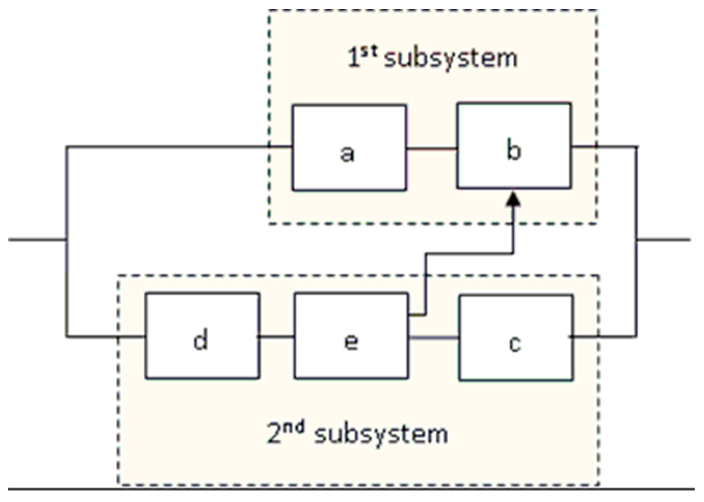
The developed optimization software tool is demonstrated as applied to the maintenance planning of a fuel pump of an aircraft jet engine. The fuel pump consists of two subsystems (subsystem 1, subsystem 2) which operate in parallel, hence for the pump to operate at least one subsystem must operate.
Subsystem 1 consists of an electrical valve (a) and a mechanical fuel regulator (b). For subsystem 1 to operate, both (a) and (b) must operate. Subsystem 2 consists of an electronic fuel regulator (c), an electrical compressor (d) and a hydraulic valve (e). For Subsystem 2 to operate, all (c), (d), and (e) must operate. In case of a failure of the electronic fuel regulator (c), Subsystem 2 can use the mechanical fuel regulator (b), which belongs to Subsystem 1.
2.1. Basic Assumptions
The fuel pump is represented by the schematic of Figure 1.
All its components operate independently and a failure of one or more components is not going to affect the operation of the rest. Furthermore, the pump can operate even when one or more of its components have failed. The first assumption here is that a component failure cannot be detected if the pump keeps operating, as such, corrective maintenance will be implemented only in case that the pump stops operating.
2.2. System Structure Function
The fuel pump structure function is:
2.3. Minimal Cut Sets
The fuel pump minimal cut sets are:
2.4. Components Reliability Functions
We accept that every component , with , is going through its useful life, hence its failure rate is constant and the respective failure intervals follow the exponential distribution with parameter . In other words, each component fails randomly and its failures follow the Poisson distribution with parameter . The reliability function of component is given by:
The component reliability information is shown in Table 2.
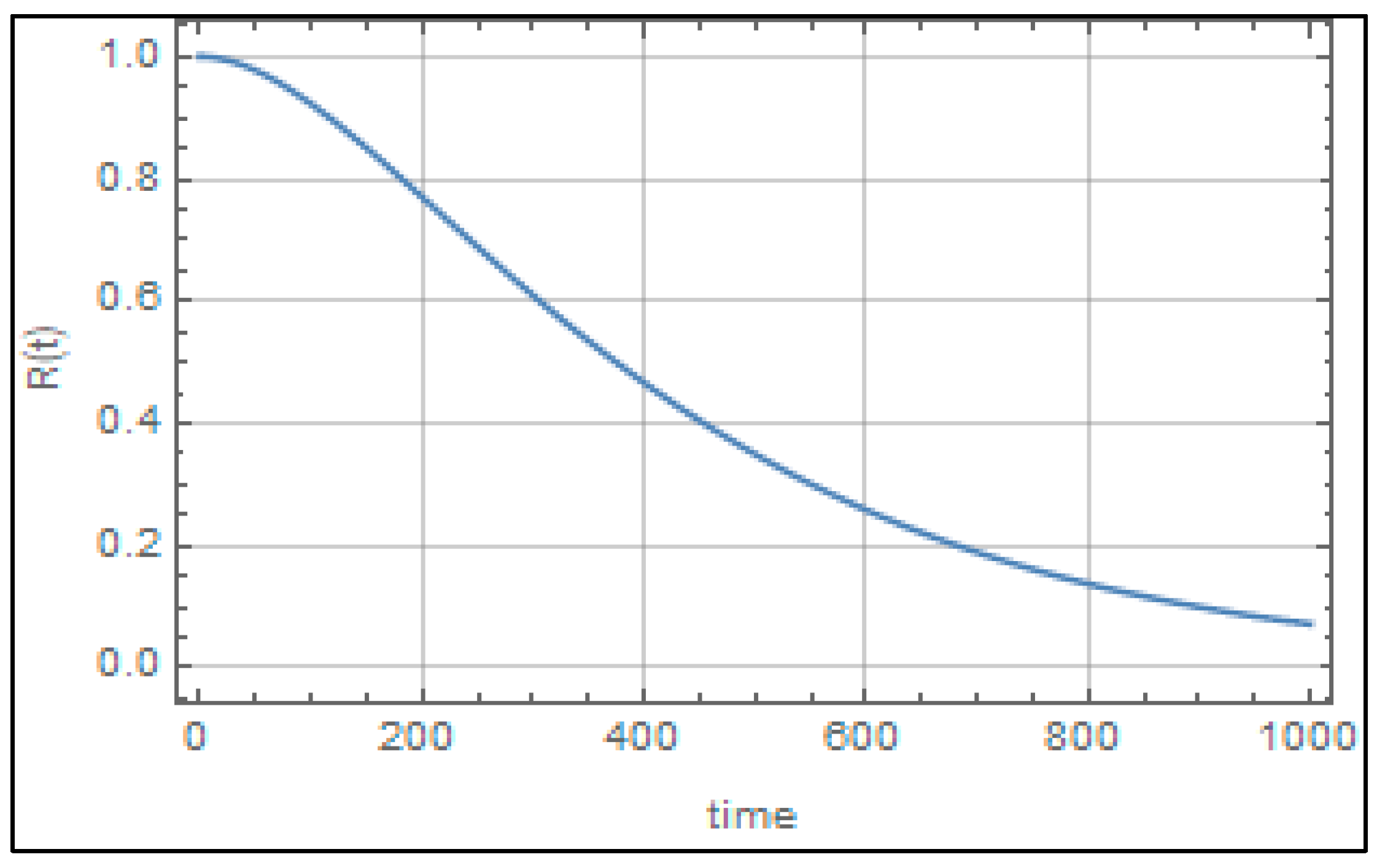
2.5. System Reliability Function
The reliability function of the fuel pump for is shown at the Figure 2 below.
At all components are assumed to be new (‘perfect’). Following Equations (13) and (14) the fuel pump reliability function is given by:
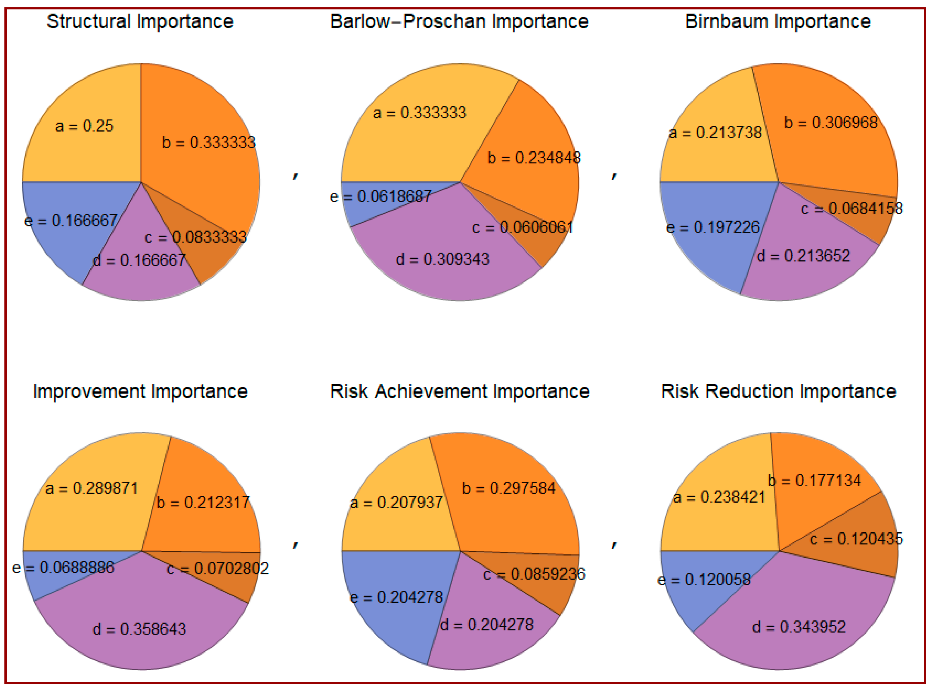
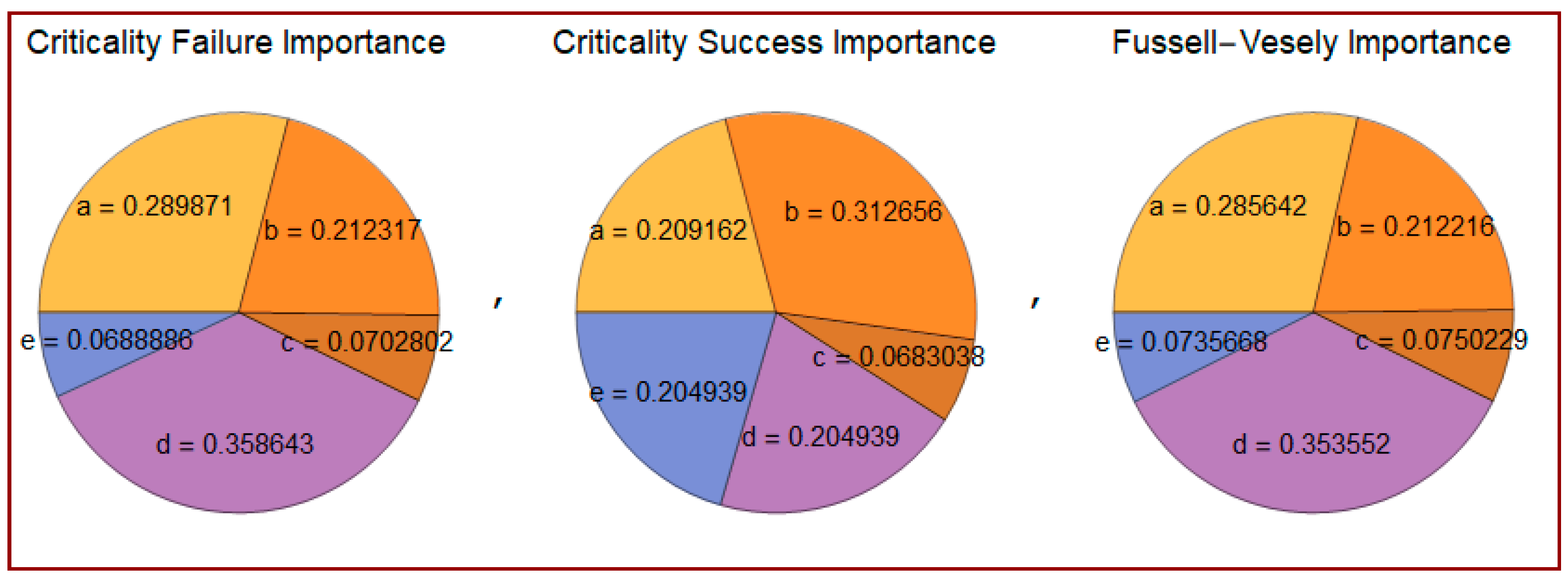
2.6. Calculation of the Components’ Importance Measures
As an example, Figure 3 shows the components’ importance measures percentages at .
Notably, the percentages of the failure-based criticality and the improvement importance measures are equal (see Proposition 1).
2.7. Estimation of the Optimum Maintenance Plan
Importance measures can be used as objective criteria to make the optimum decision regarding the maintenance planning of the fuel pump. However, since the importance measures do not consider the associated cost of components, we introduce a cost adjustment. Thus, we expand the applicability of the importance measures as a ‘benefit over cost’ criterion for decision making, while trying to determine the optimum maintenance scenario.
2.7.1. Inputs
The proposed software tool uses the following inputs:
- The structure of the system.
- The life cycle of the system, more specifically the timeframe of the maintenance plan of the system.
- The reliability distribution of each component.
- The importance measure which is going to be used as an objective criterion to determine the component which will be replaced on a preventive basis during the implementation of the scheduled maintenance of the system. The specified importance measure will be cost-adjusted according to the cost inputs that follow.
- The cost of the scheduled preventive replacement of each component with a brand new one. In other words, the cost of scheduled preventive maintenance for each component after which the cumulative time of operation of the component is zero.
- The cost of the nonscheduled replacement of each component with a brand new one. In other words, the cost of nonscheduled maintenance for each component after which the cumulative time of operation of the component is zero.
- The cost of scheduled preventive replacement of all the components, at once, with brand new ones. In other words, the cost of scheduled preventive maintenance for all components simultaneously, after which the cumulative time of operation of the components is zero.
- The confidence level for the fulfilment of the nonscheduled maintenance requirements, in case of system failures.
2.7.2. Processing
The software tool will use an algorithm to assess all the potential scheduled maintenance scenarios; for each scenario it will calculate the value of the criterion ‘lowest total maintenance cost/average reliability outcome’. The lowest value of the criterion will determine the optimum scheduled maintenance scenario. Specifically, the structure of the algorithm is:
| Estimate system structure function For N = 0 to 98:
|
2.7.3. Outputs
The outputs of the tool are the following:
- The diagram of the procedure for which the lowest value of the criterion ‘cost/benefit’ is achieved.
- The reliability function diagram of the system for the optimum scheduled maintenance scenario.
- The average reliability of the system.
- The lowest value of the reliability of the system, at which the system has to be grounded for scheduled maintenance.
- The MTTF of the system.
- The replacement schedule for the system’s components.
- The required number of spare parts for each component, for both scheduled and nonscheduled maintenance (at the determined confidence level).
- The cost analysis for both scheduled and nonscheduled replacement of the components.
3. Exemplified Example/Results
The following is an exemplified example of an optimization process that uses the proposed software tool.
3.1. Task
The optimum maintenance plan for the fuel pump needs to be established for its first 3000 h of operation with the following constraints: Only one component will be replaced by a new one (or its cumulative time of operation will be considered as zero following an inspection/rectification) during the implementation of the scheduled maintenance of the system. The criterion that will determine the component to be replaced is the ‘cost-adjusted improvement importance measure’, which corresponds to the cost of the scheduled replacement of each individual component, as illustrated in Table 2.
3.2. Components Replacement Cost
The replacement cost of the components is estimated for three different cases:
- Scheduled replacement of a unique component (preventive maintenance)
- Nonscheduled replacement of a unique component (corrective maintenance)
- Scheduled replacement of all the components simultaneously (preventive maintenance)
The estimation of the scheduled replacement cost for each component takes into account the purchase price of the component and of all the consumables required for its replacement, as well as the total cost of the required maintenance work, such as depreciation of special tools and equipment, energy cost, man-hours cost, the system down-time and its effect on the operational availability, as well as any other associated cost (safe maintenance procedures cost, accessibility cost, operational checks cost, transportation cost for involved staff and materiel).
The cost of the nonscheduled replacement of each component in case of a pump failure should be considered higher than the respective scheduled replacement cost. Further to the cost categories which have been mentioned previously, the risk of unintended damage and/or failures of other jet engine subsystems due to the failure of the pump, should also be considered. It is also possible that the fuel pump fails in a location at a distance from the maintenance base station, a situation that will potentially incur higher costs and disruption to the aircraft fleet operations, due to the nonscheduled grounding of the jet engine and, consequently, the aircraft.
The information regarding the replacement cost (scheduled and nonscheduled) of each component of the fuel pump is presented at the Table 2.
The estimation of the replacement cost, at once, of more than one components, should consider the fact that the total replacement cost should be less than the sum of the scheduled replacement cost for each component (Table 2). This is due to the economies of scale, which materialize due to maintenance work which is common for some or all the components. For example, when all the components are replaced at once, safe maintenance procedures and the operational check of the fuel pump take place only once. In addition, the total downtime of the pump is less and the cumulative effect to the operational availability of the jet engines/aircraft fleet is less severe.
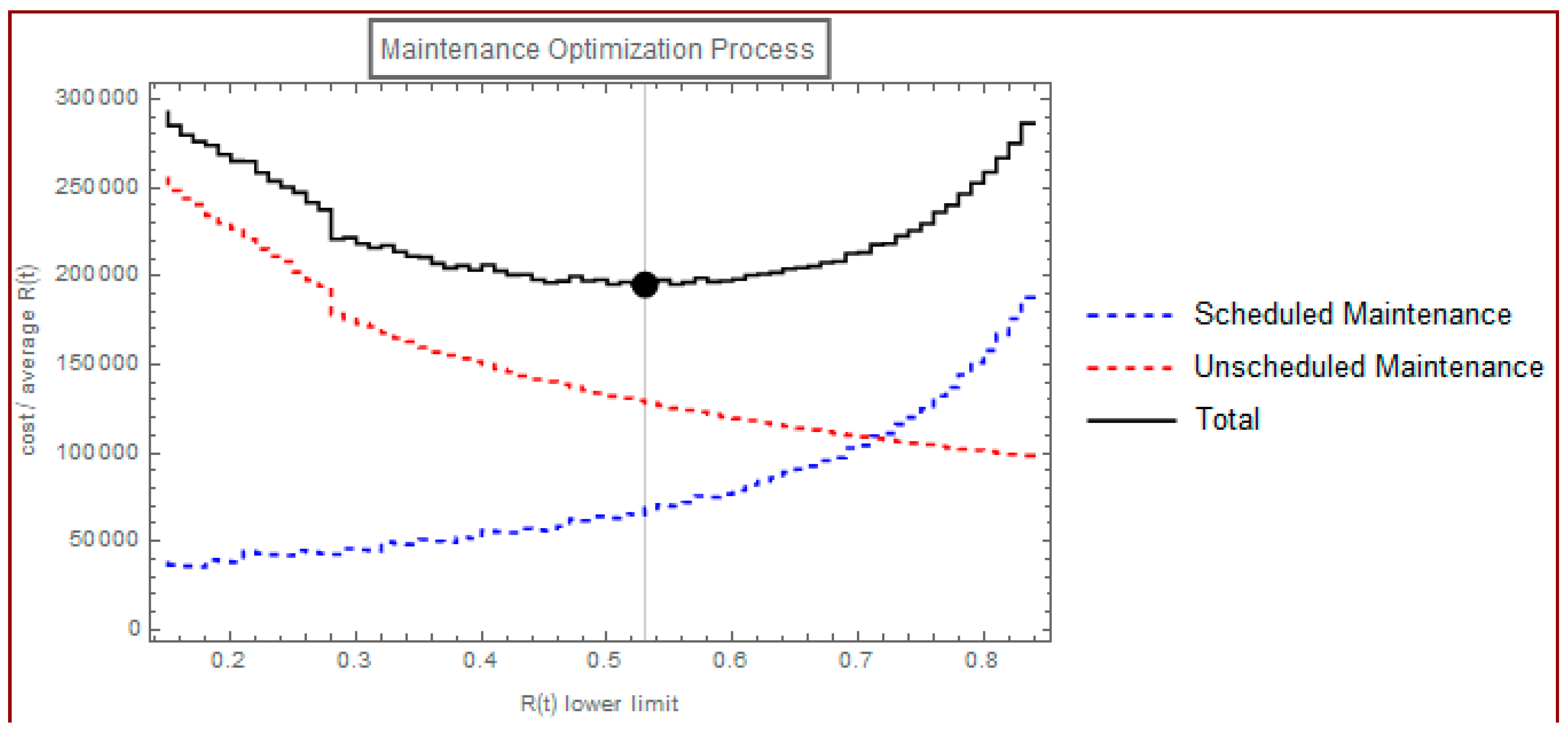
3.3. Optimization Criterion
As optimum maintenance plan is considered the one with the lowest possible total maintenance cost (for both scheduled and nonscheduled maintenance) for the average reliability, which is achieved during the first 3000 h of operation of the fuel pump. In other words, the optimization criterion is the lowest possible value of ‘cost over benefit’. The optimization of the preventive maintenance plan is shown in Figure 4.
3.4. Optimum Number of Spare Components for Scheduled Maintenance
Every time that the reliability of the fuel pump approaches the lowest acceptable limit, the pump is grounded for scheduled maintenance. In that case, a preventive replacement will take place for the component for which it is estimated to achieve the highest possible improvement of the reliability of the pump for the associated cost of the improvement. The importance measure of the improvement is actually ‘cost adjusted’ and as such the decision which has been made is to replace the component for which the lowest value of ‘cost/benefit’ is achieved.
More specifically, if at the time of the scheduled downtime, the value of the improvement importance measure for the component is , with , and the replacement cost of each component is , then, as shown in Table 2, the component replaced is not the one with the highest value of , but the one with the highest value of . This is how an estimation can be made for the complete list of the components which are going to be replaced during the first 3000 h of operation of the pump. Having assessed that, an estimation can be made as well for the number of spare components which will be needed for the scheduled maintenance of the pump.
3.5. Optimum Number of Spare Components for Non-Scheduled Maintenance
The mean time between two successive occurrences of nonscheduled maintenance for the first 3000 h of operation of the fuel pump can be estimated by Equation (3) as MTTF = 2040.3 h. The number of failures is: μ = 8.26.
The number of failures, for a certain confidence level, and the respective number of spare components needed for the nonscheduled maintenance for the first 3000 h of operation can be estimated by using Poisson distribution with parameter μ = 8.26. As per the results presented at the Table 3 (for a 95% confidence level), a number of 13 nonscheduled component replacements will be needed for a single fuel pump.
Having estimated this, the quantity of each specific type of spare part for the corrective maintenance can now be estimated. This time, the failure-based criticality importance measure is considered to better express the contribution of each type of spare component to the occurrence of a fuel pump failure. This importance measure represents the probability of a fuel pump failure due to a component failure. Equivalently, according to the Proposition 1, the (more conveniently estimated) improvement importance measure can be used as well.
For the occasion of unscheduled maintenance requirements, cost adjustment on the improvement importance measure is not required. Indeed, cost does not affect the probability of fuel pump failure due to a specific component failure. However, since the improvement importance measure is now applied through the whole 3000 operational hours timeframe, and not to a specific instance in time (such as in the case of scheduled maintenance temporal points), the integral of the improvement importance measure for every component is calculated, from 0 to 3000 h of the pump’s operation. The integration of the improvement importance measures serves as the allocation base for the previously estimated total 13 spare components (unscheduled maintenance), in order to determine the quantity for each component type.
After the allocation of the 13 system failures to each spare part, it is strongly recommended that no rounding should be performed for a single fuel pump’s spares (as seen in Table 3). Such an analysis normally aims at making provisions for a relatively large population of fuel pumps, hence it is suggested that any rounding should be performed after the calculation of the total number of each spare part type.
Table 3 shows that a confidence level of 95% to fulfill the nonscheduled maintenance requirements of the pump for the first 3000 h of operation, is going to require 13 spare components. Using the integral of the improvement importance measure as an allocation basis for the 13 spare components, it is concluded that five nonscheduled replacements of component (a) are going to take place), 4.4 nonscheduled replacements of the component (b), 0.5 nonscheduled replacements of the component (c), 2.7 nonscheduled replacements of the component (d) and 0.5 nonscheduled replacements of the component (e). The total cost of all the above nonscheduled replacements is 88,817.70 , and this is the total cost of the nonscheduled maintenance of the pump for the first 3000 h of operation.
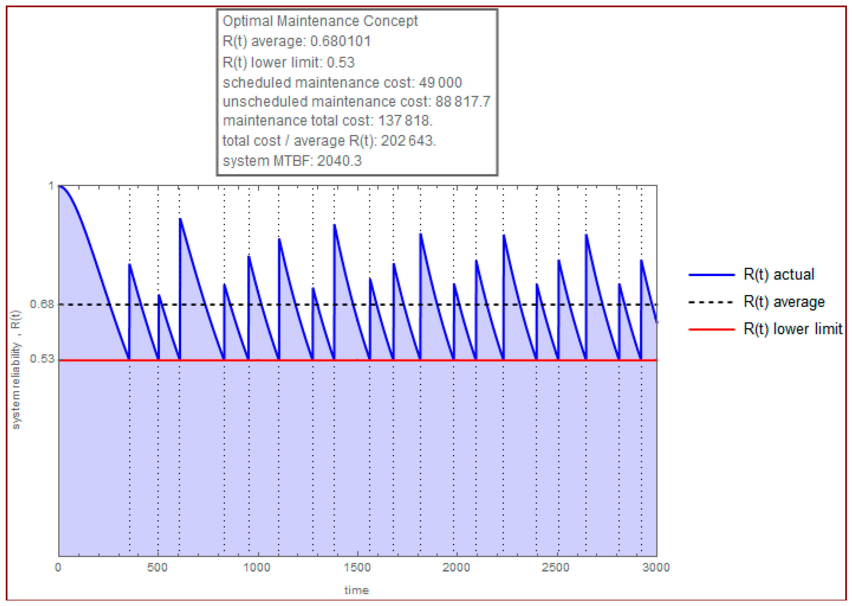
3.6. Results
The reliability function of the first 3000 h of operation of the fuel pump is presented in Figure 5. The local maxima of the curve represent the improvement of the reliability of the fuel pump following the scheduled down time during which a preventive replacement of a component has taken place. It is reminded that the decision to replace a component has been made based to the lowest value of the cost/benefit optimization criterion, using the cost-adjusted improvement importance measure.
The horizontal red line shows the lowest acceptable reliability limit for the fuel pump, which is 53%. Whenever the limit is reached, the pump is grounded for preventive maintenance or replacement of a specific component. The horizontal dotted black line shows the mean reliability of 68%, which is achieved during the 3000 h of operation.
The results shown in Table 4 and Table 5 indicate that fulfilling the scheduled maintenance requirements of the first 3000 h of operation, is going to require 11 stand-alone replacements of the component (a), seven stand-alone replacements of the component (b) and one stand-alone replacement of the component (d). The total cost of all the above replacements is 49,000 and this is the total cost of the scheduled maintenance of the pump for the first 3000 h of operation. Notably, no PCRs for components (c) and (e) are required, because any potential replacement of these components would have brought relatively poor improvement in the fuel pump’s reliability, given the associated replacement cost. On the other hand, Table 5 shows that the components (a) and (b) PCRs usually have the highest impact on the fuel pump’s reliability improvement, compared to the associated replacement cost.
The total maintenance cost (scheduled and nonscheduled) can now be calculated for the first 3000 operation hours of the pump:
and the mean reliability for the same timeframe is 68%. As such, the optimization criterion of (cost/benefit) takes its optimum value of .
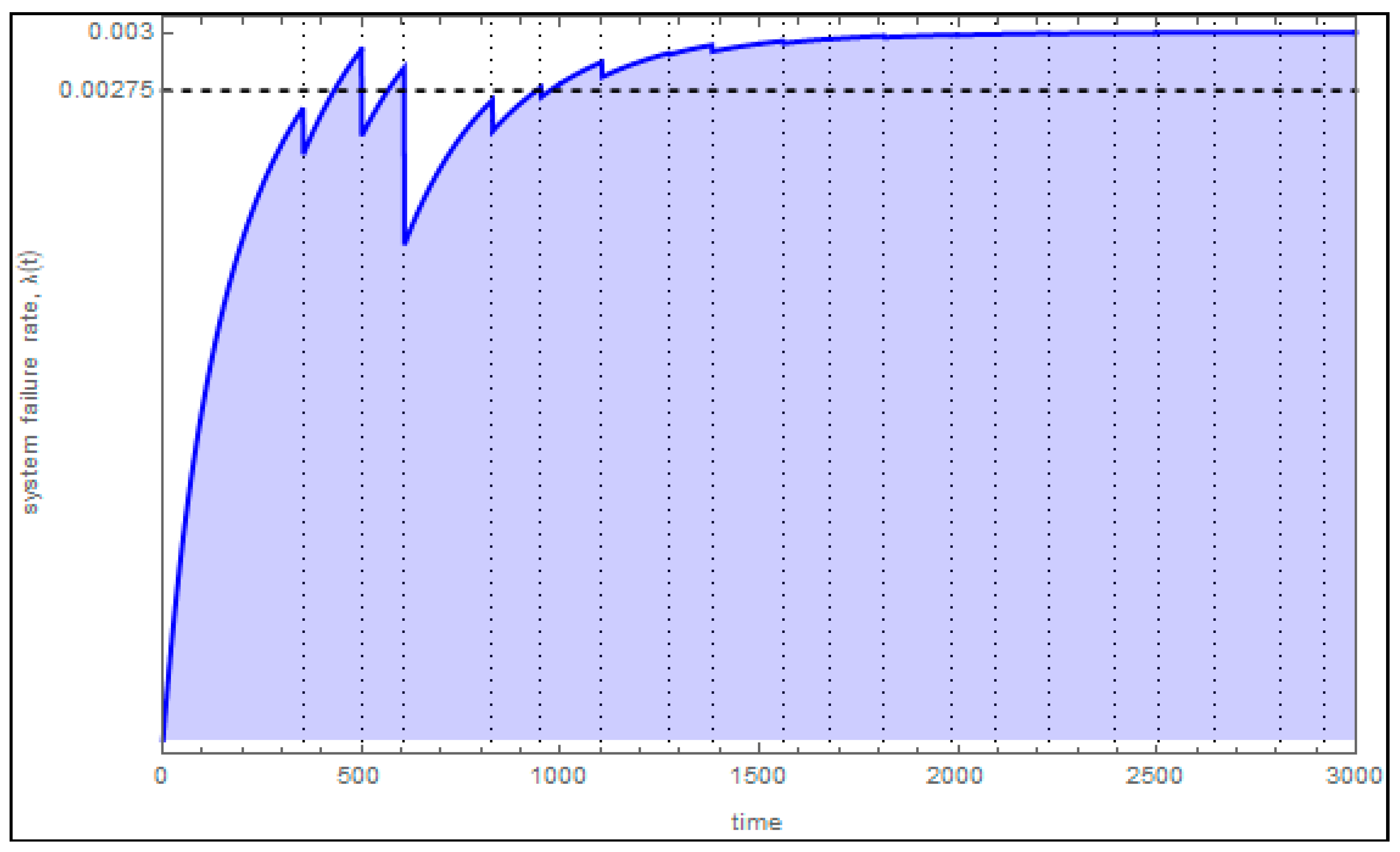
Figure 6 shows the failure rate and the mean failure rate of the fuel pump.
It is observed that after the first 1500 h of operation, which seems as a ‘warm-up period’, the failure rate of the pump converges to a constant value (CFR period).
3.7. An Alternative Scenario: All Components Are Replaced Simultaneously
At this scenario, all the components are replaced simultaneously at any time the pump is subjected to scheduled maintenance. Still, the timing of the scheduled maintenance is determined by the lowest reliability limit which has been set for the pump. After each time the pump is subjected to scheduled maintenance, the pump is considered as brand new and, as such, the time interval between two subsequent scheduled maintenance occurrences is considered as constant.
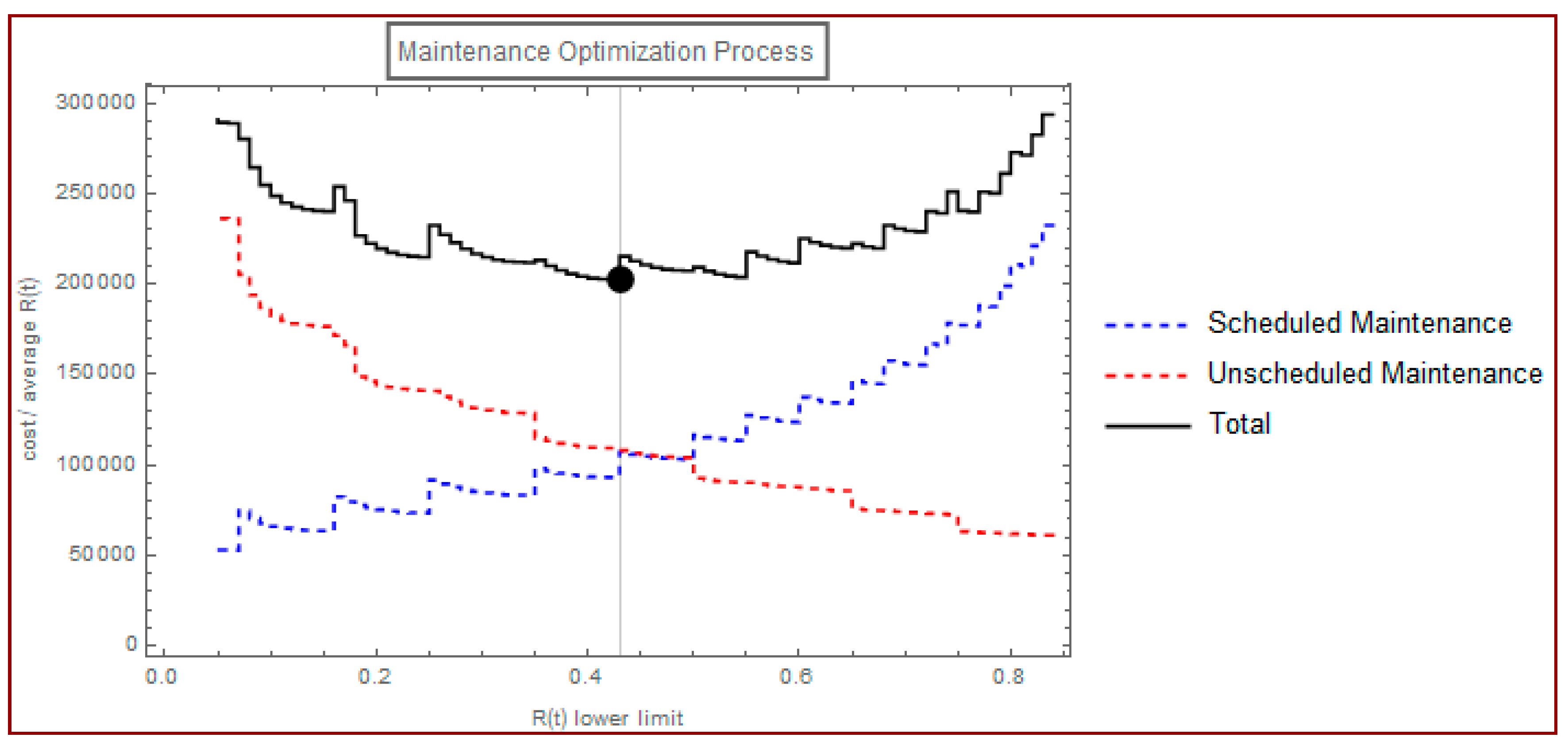
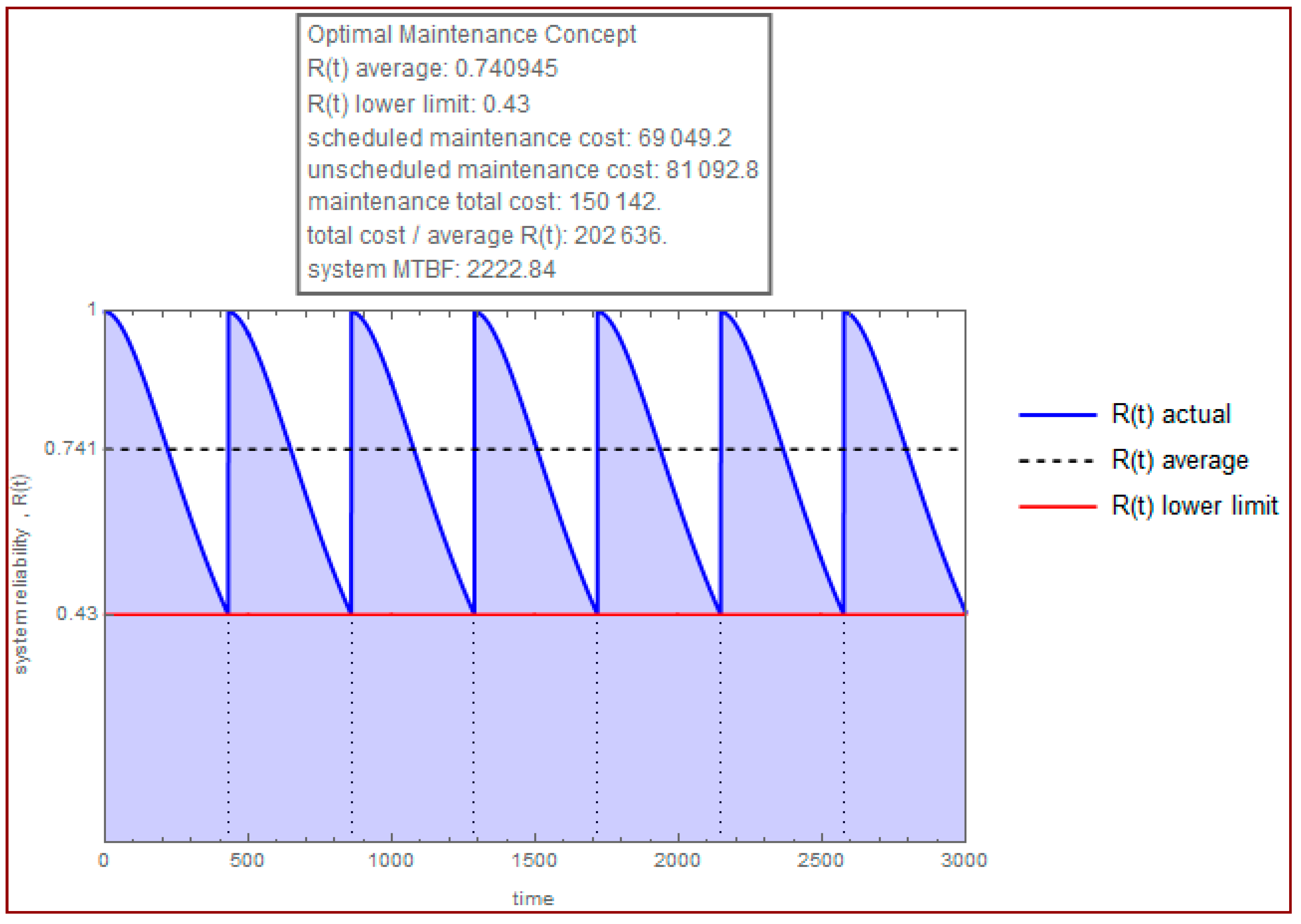
The optimization of the maintenance plan for this alternative scenario is shown at the Figure 7.
Following this, the developed software tool investigates thoroughly the optimum maintenance plan and returns to Figure 8 as well as Table 6, Table 7 and Table 8.
According to the assumption of Section 3.2, the cost of the scheduled replacement of more than one components simultaneously, is going to be less than the sum of the costs of each stand-alone scheduled replacement as shown in Table 2. More specifically, it is deducted that since the cost of the preventive simultaneous replacement of all the components is less than the 52.31% of the sum of the costs of each stand-alone preventive replacement, then the scenario of the preventive replacement of all the components simultaneously is more efficient. In case the scheduled simultaneous replacement of all the components maintains the cost at 52.31%, as compared with the original scenario, then the two scenarios are almost equivalent with regards to the optimization criterion being used. Of note, the case under examination serves as an example for the application of the software tool; no actual data were used, including the system structure, components reliability functions, and component replacement costs. The equivalence threshold is sensitive to structure, reliability, and cost inputs—hence the above-estimated 52.31% threshold should not be generalized.
Table 6 results indicate that the optimum maintenance is achieved when the pump is grounded every h of operation and all its components are replaced at once, with reliability approaching the lowest acceptable limit of 43%.
Table 7 shows that to fulfil the preventive maintenance requirements of the pump during its first 3000 h of operation, six components of each type need to be scheduled to be replaced. In that case, the total replacement cost of the 30 involved components is . For this alternative scenario, this is the total cost of the preventive maintenance of the pump for the first 3000 h of operation.
Table 8 shows that, a confidence level of 95% to fulfil the nonscheduled maintenance requirements for the first 3000 h of operation of the fuel pump, is going to require a nonscheduled replacement of 10 components. In more detail, the alternative scenario is going to require the nonscheduled replacement of 3.2 (a) components, 1.98 (b) components, 0.62 (c) components, 3.66 (d) components and 0.54 (e) components. The total cost of all the above nonscheduled replacements is 81,092.8 , and this is the total cost of the nonscheduled maintenance of the pump for the first 3000 h of operation.
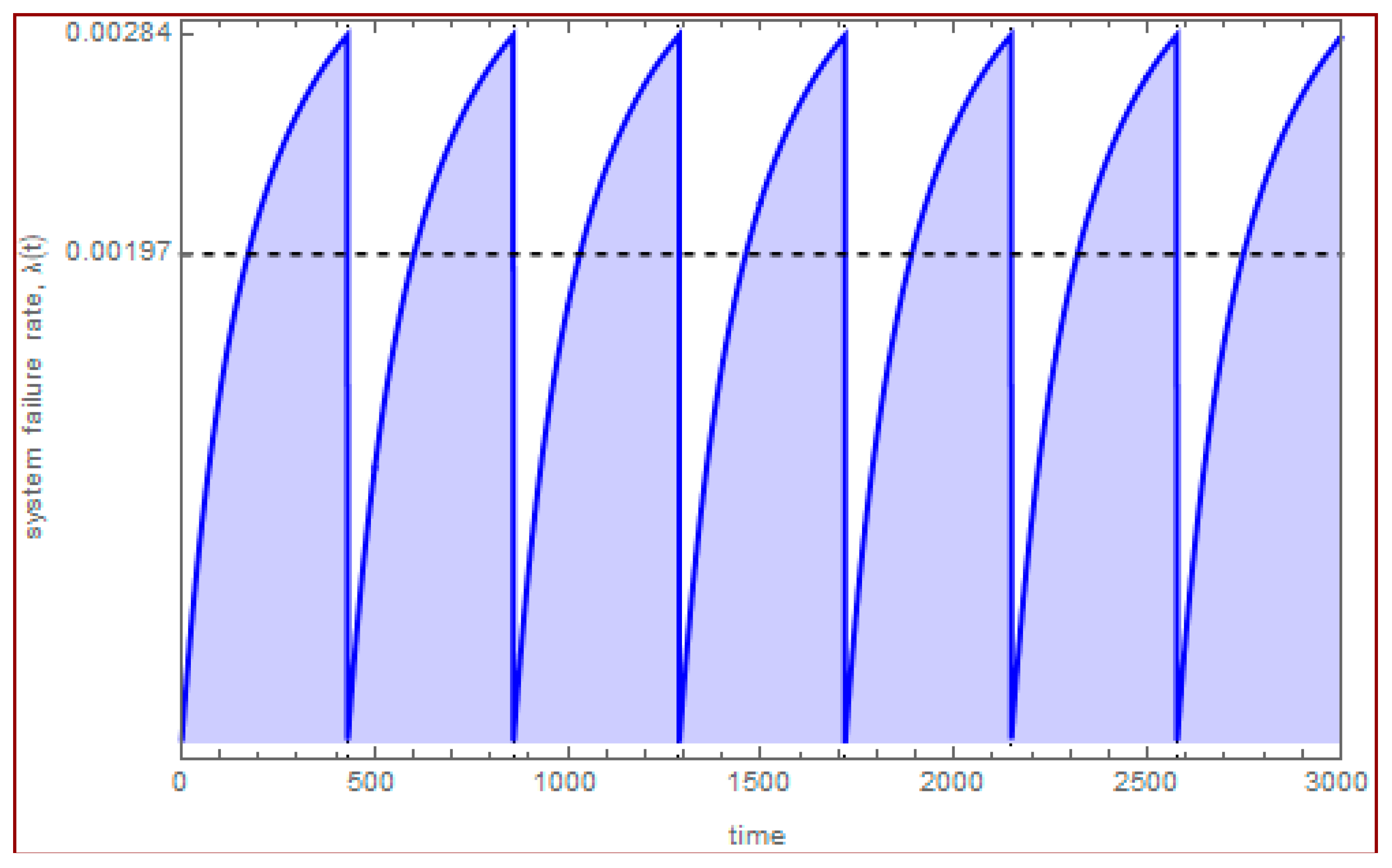
Figure 9 shows the failure rate and the mean failure rate . The failure rate takes its highest value just before the scheduled grounding of the pump. Another observation is that between two successive groundings, the pump is always at IFR period.
The total maintenance cost (scheduled and nonscheduled) can now be calculated for the first 3000 operation hours of the pump:
and the mean reliability for the same timeframe is 74.1%. As such, the optimization criterion of cost/benefit takes its optimum value of . The value is almost equivalent to the value of the optimization criterion of the first scenario.
The outputs of the two maintenance concepts are summarized in Table 9.
4. Discussion
Combination of dependencies and simulation optimization have been considered as promising areas for future work for optimal maintenance of multicomponent systems [26]. On the other hand, most optimal maintenance models in the literature use as optimization criterion the system maintenance cost rate, but they ignore the reliability performance [27]. Minimizing the system maintenance cost rate does not necessarily imply that the system reliability performance is optimized with regards to the cost, especially for multicomponent systems, and sometimes minimal maintenance cost is associated with very low system reliability measures. This is one of the effects of having various components in the system which may have different maintenance costs and different importance for the system [28]. As such, the optimal maintenance should always take into account both the maintenance cost and reliability and this is the rationale of introducing the cost adjusted importance measure to determine the optimal maintenance plan.
In the specific example of the fuel pump, it is noticeable that the first scenario (replacement of one component at a time) essentially brings the fuel pump at a state of a constant failure rate, after a ‘warmup’ period. On the contrary, the alternative scenario (simultaneous replacement of all components) does not have the same effect on the failure rate. Further investigation is needed, in order to assess the mechanism behind the convergence of the failure rate of the first scenario.
Other preventive maintenance scenarios may be examined as well, for example the simultaneous replacement of two or more components, at each time the pump is grounded for scheduled maintenance. In such cases, the calculation of combined importance measures is required.
Furthermore, the required confidence level for the number of components spare parts, which are required for the nonscheduled maintenance, affects the respective maintenance cost. This is a key cost driver for the maintenance optimization process; it is also a risk source for potential availability shortfalls, therefore careful attention should be paid to determine an appropriate confidence level.
Author Contributions
M.B. contributed to the data curation and all authors contributed to the conceptualization, project administration, formal analysis, writing, editing and reviewing the manuscript.
Funding
This research received no external funding.
Conflicts of Interest
The authors declare no conflicts of interest.
References
- Samaranayake, P.; Kiridena, S. Aircraft maintenance planning and scheduling: An integrated framework. J. Qual. Maint. Eng. 2012, 18, 432–453. [Google Scholar] [CrossRef]
- Rosenzweig, V.V.; Domitrovic, A.; Bubic, M. Planning of training aircraft flight hours. Croat. Oper. Res. Rev. (CRORR) 2010, 1, 170–179. [Google Scholar]
- Kozanidis, G.; Gavranis, A.; Kostarelou, E. Mixed integer least squares optimization for flight and maintenance planning of mission aircraft. Naval Res. Logist. 2012, 59, 212–229. [Google Scholar] [CrossRef]
- Gavranis, A.; Kozanidis, G. An exact solution for maximizing the fleet availability of a unit of aircraft subject to flight and maintenance requirements. Eur. J. Oper. Res. 2015, 242, 631–643. [Google Scholar] [CrossRef]
- Antonakis, A.S.; Giannakoglou, K.C. Optimization of military aircraft engine maintenance subject to engine part shortages using asynchronous metamodel-assisted particle swarm optimization and Monte-Carlo simulations. Int. J. Syst. Sci. Oper. Logist. 2017. [Google Scholar] [CrossRef]
- Papakostas, N.; Papachatzakis, P.; Xanthakis, V.; Mourtzis, D.; Chryssolouris, G. An approach to operational aircraft maintenance planning. Decis. Support Syst. 2010, 48, 604–612. [Google Scholar] [CrossRef]
- Cheung, A.; Ip, W.H.; Lu, D. Expert system for aircraft maintenance services industry. J. Qual. Maint. Eng. 2005, 11, 348–358. [Google Scholar] [CrossRef]
- Joo, S.J. Scheduling preventive maintenance for modular designed components: A dynamic approach. Eur. J. Oper. Res. 2009, 192, 512–520. [Google Scholar] [CrossRef]
- Gustavsson, M.P.; Patriksson, M.; Stomberg, A.B.; Wojciechowski, A.; Onnheim, M. Preventive maintenance scheduling of multi-component systems with interval costs. Comput. Ind. Eng. 2014, 76, 390–400. [Google Scholar] [CrossRef]
- Vianna, W.O.L.; Yoneyama, T. Predictive maintenance optimization for aircraft redundant systems subjected to multiple wear profiles. IEEE Syst. J. 2018, 12, 1170–1181. [Google Scholar] [CrossRef]
- Office of the Secretary of Defense. Cost Assessment and Program Evaluation; Office of the Secretary of Defense: Washington, DC, USA, 2014.
- Department of Defense. MIL-STD-3034 ‘Reliability-Centered Maintenance (RCM) Process’; Department of Defense: Washington, DC, USA, 2011.
- Wojciechowski, A. On the Optimization of Opportunistic Maintenance. Thesis for the Degree of Licentiate of Engineering, Chalmers University of Gothenburg, Gothenburg, Sweden, 2010. [Google Scholar]
- Deputy under Secretary for Logistics and Materiel Readiness. Memorandum ‘Condition Based Maintenance Plus; Deputy under Secretary for Logistics and Materiel Readiness: Washington, DC, USA, 2002.
- SAE JA1011 ‘Evaluation criteria for Reliability-Centered Maintenance Processes; SAE International: Warrendale, PA, USA, 2009.
- API Recommended Practice 580 ‘Risk Based Inspection; American Petroleum Institute: Washington, DC, USA, 2016.
- Chairman of the Joint Chiefs of Staff Manual. CJCSM 3170.01C ‘Operation of the Joint Capabilities Integration and Development System’; Chairman of the Joint Chiefs of Staff Manual: Washington, DC, USA, 2017. [Google Scholar]
- Cheok, M.C.; Parry, G.W.; Sherry, R.R. Use of importance measures in risk-informed regulatory applications. Reliab. Eng. Syst. Saf. 1998, 60, 213–226. [Google Scholar] [CrossRef]
- Vasseur, D.; Llory, M. International survey on PSA figures of merit. Reliab. Eng. Syst. Saf. 1999, 66, 261–274. [Google Scholar] [CrossRef]
- Van Der Borst, M.; Schoonakker, H. An overview of PSA importance measures. Reliab. Eng. Syst. Saf. 2001, 72, 241–245. [Google Scholar] [CrossRef]
- Vaurio, J.K. Ideas and developments in importance measures and fault-tree techniques for reliability and risk analysis. Reliab. Eng. Syst. Saf. 2010, 95, 99–107. [Google Scholar] [CrossRef]
- Vaurio, J.K. Importance measures in risk-informed decision making: Ranking, optimization and configuration control. Reliab. Eng. Syst. Saf. 2011, 96, 1426–1436. [Google Scholar] [CrossRef]
- Rocco, C.M.; Ramirez-Marquez, J.E. Innovative approaches for addressing old challenges in component importance measures. Reliab. Eng. Syst. Saf. 2012, 108, 123–130. [Google Scholar] [CrossRef]
- Wolfram Language and System Documentation Center. Available online: http://reference.wolfram.com/language/ (accessed on 25 May 2018).
- Leemis, L.M. Reliability: Probabilistic Models and Statistical Methods; Prentice Hall, Inc.: Englewood Clifs, NJ, USA, 1995; ISBN 9780137205172. [Google Scholar]
- Nicolai, R.P.; Dekker, R. Optimal Maintenance of Multi-Component Systems: A Review; Erasmus University Rotterdam, Erasmus School of Economics: Rotterdam, The Netherlands, 2006. [Google Scholar]
- Wang, H. A survey of maintenance policies of deteriorating systems. Eur. J. Oper. Res. 2002, 139, 469–489. [Google Scholar] [CrossRef]
- Wang, H.; Pham, H. Availability and optimal maintenance of series systems subject to imperfect repair and correlated failure and repair. Eur. J. Oper. Res. 2006, 17, 1706–1722. [Google Scholar] [CrossRef]
Figure 1.
Schematic of the fuel pump.

Figure 2.
Reliability function of the fuel pump for .

Figure 3.
Components’ importance measures percentages at .


Figure 4.
Optimization of the preventive maintenance plan for the fuel pump for the first 3000 h of its operation.
Figure 4.
Optimization of the preventive maintenance plan for the fuel pump for the first 3000 h of its operation.

Figure 5.
The reliability function under the optimum maintenance plan for the fuel pump for its first 3000 h of operation.
Figure 5.
The reliability function under the optimum maintenance plan for the fuel pump for its first 3000 h of operation.

Figure 6.
Failure rate (blue curve) and the mean failure rate (horizontal dotted line) of the fuel pump for its first 3000 h of operation.
Figure 6.
Failure rate (blue curve) and the mean failure rate (horizontal dotted line) of the fuel pump for its first 3000 h of operation.

Figure 7.
Optimization of the preventive maintenance plan for the fuel pump for the first 3000 h of its operation (alternative scenario).
Figure 7.
Optimization of the preventive maintenance plan for the fuel pump for the first 3000 h of its operation (alternative scenario).

Figure 8.
Fuel pump reliability for the first 3000 h of its operation (alternative scenario).

Figure 9.
Failure rate (blue curve) and the mean failure rate (horizontal dotted line) of the pump for its first 3000 h of its operation (alternative scenario).
Figure 9.
Failure rate (blue curve) and the mean failure rate (horizontal dotted line) of the pump for its first 3000 h of its operation (alternative scenario).


Table 1.
Notations for the basic functions.
| Notation | Description |
|---|---|
| System reliability function | |
| System unreliability function | |
| Component reliability function | |
| Component unreliability function | |
| System reliability function, whereas (perfect component ) | |
| System reliability function, whereas (failed component ) | |
| System unreliability function, whereas (perfect component ) | |
| System unreliability function, whereas (failed component ) |
Table 2.
Component reliability and cost information.
| Component MTTF (Hours) | Component Failure Rate (Constant) | Component Reliability Function | Cost of Scheduled Replacement of a Single Component (Euros) | Cost of Unscheduled Replacement of a Single Component (Euros) |
|---|---|---|---|---|
Table 3.
Spare components required to fulfil the nonscheduled maintenance requirements (95% confidence level).
Table 3.
Spare components required to fulfil the nonscheduled maintenance requirements (95% confidence level).
| Part Type | Items | Cost |
|---|---|---|
| A | 5.02131 | 20,085.20 |
| B | 4.36118 | 26,167.10 |
| C | 0.462472 | 3699.78 |
| D | 2.6525 | 31,830.00 |
| E | 0.502543 | 7035.60 |
| Fails | ||
| (95.7391%) | 13 | 88,817.70 |
Table 4.
Components replacement plan for the scheduled maintenance of the fuel pump for its first 3000 h of operation.
Table 4.
Components replacement plan for the scheduled maintenance of the fuel pump for its first 3000 h of operation.
| Part Type | Replace at |
|---|---|
| d | 353.653 |
| b | 500.406 |
| a | 607.353 |
| a | 829.207 |
| b | 951.600 |
| a | 1104.010 |
| b | 1273.250 |
| a | 1381.720 |
| a | 1560.730 |
| b | 1678.180 |
| a | 1813.860 |
| a | 1981.150 |
| b | 2092.210 |
| a | 2230.450 |
| a | 2396.240 |
| b | 2506.640 |
| a | 2644.860 |
| a | 2810.480 |
| b | 2920.860 |
Table 5.
Total replacement cost breakdown for the scheduled maintenance of the fuel pump for its first 3000 h of operation.
Table 5.
Total replacement cost breakdown for the scheduled maintenance of the fuel pump for its first 3000 h of operation.
| Part Type | Items | Cost |
|---|---|---|
| a | 11 | 22,000 |
| b | 7 | 21,000 |
| c | 0 | 0 |
| d | 1 | 6000 |
| e | 0 | 0 |
| Total sched. | 19 | 49,000 |
Table 6.
Components replacement plan (alternative scenario).
| Part Types | Replace at |
|---|---|
| a, b, c, d, e | 429.21 |
| a, b, c, d, e | 858.42 |
| a, b, c, d, e | 1287.64 |
| a, b, c, d, e | 1716.85 |
| a, b, c, d, e | 2146.06 |
| a, b, c, d, e | 2575.27 |
Table 7.
Total replacement cost breakdown (alternative scenario).
| Part Type | Items | Cost |
|---|---|---|
| a | 6 | |
| b | 6 | |
| c | 6 | |
| d | 6 | |
| e | 6 | |
| Total sched. | 30 | 69,049.20 |
Table 8.
Total replacement cost breakdown (alternative scenario, confidence level 95%).
| Part Type | Items | Cost |
|---|---|---|
| a | 3.200540 | 12,802.10 |
| b | 1.983480 | 11,900.90 |
| c | 0.618516 | 4948.13 |
| d | 3.661420 | 43,937.10 |
| e | 0.536043 | 7504.60 |
| Fails. | 10 | 81,092.80 |
Table 9.
Summary of the two maintenance concepts.
| Initial Scenario | Alternative Scenario | |||||
| Average reliability | 0.68 | 0.74 | ||||
| Reliability lower limit | 0.53 | 0.43 | ||||
| Cost of scheduled maintenance | 49,000 | 69,049 | ||||
| Cost of unscheduled maintenance | 88,817 | 81,093 | ||||
| Total maintenance cost | 137,818 | 150,142 | ||||
| Total maintenance cost/average reliability | 202,643 | 202,636 | ||||
| Average failure rate per 1000 h of operation | 2.75 | 1.97 | ||||
| MTTF | 2040 | 2223 | ||||
| Component Types | Sched. | Unsched. | Total | Sched. | Unsched. | Total |
| A | 11 | 5.0 | 16.0 | 6 | 3.2 | 9.2 |
| B | 7 | 4.4 | 11.4 | 6 | 2.0 | 8.0 |
| c | 0.5 | 0.5 | 6 | 0.6 | 6.6 | |
| d | 1 | 2.7 | 3.7 | 6 | 3.7 | 9.7 |
| e | 0.5 | 0.5 | 6 | 0.5 | 6.5 | |
| Total | 19 | 13 | 32 | 30 | 10 | 40 |
© 2018 by the authors. Licensee MDPI, Basel, Switzerland. This article is an open access article distributed under the terms and conditions of the Creative Commons Attribution (CC BY) license (http://creativecommons.org/licenses/by/4.0/).
Share and Cite
MDPI and ACS Style
Bozoudis, M.; Lappas, I.; Kottas, A. Use of Cost-Adjusted Importance Measures for Aircraft System Maintenance Optimization. Aerospace 2018, 5, 68. https://0-doi-org.brum.beds.ac.uk/10.3390/aerospace5030068
AMA Style
Bozoudis M, Lappas I, Kottas A. Use of Cost-Adjusted Importance Measures for Aircraft System Maintenance Optimization. Aerospace. 2018; 5(3):68. https://0-doi-org.brum.beds.ac.uk/10.3390/aerospace5030068
Chicago/Turabian StyleBozoudis, Michail, Ilias Lappas, and Angelos Kottas. 2018. "Use of Cost-Adjusted Importance Measures for Aircraft System Maintenance Optimization" Aerospace 5, no. 3: 68. https://0-doi-org.brum.beds.ac.uk/10.3390/aerospace5030068
Note that from the first issue of 2016, this journal uses article numbers instead of page numbers. See further details here.