Fast Evaluation of Aircraft Icing Severity Using Machine Learning Based on XGBoost


1
Department of Mechanical and Industrial Engineering, University of Illinois at Chicago, Chicago, IL 60607, USA
2
Department of Computer Science, Beijing University of Posts and Telecommunications, Beijing 100083, China
3
National Oilwell Varco, Houston, TX 77041, USA
4
Computational Science Division and Leadership Computing Facility, Argonne National Laboratory, Lemont, IL 60439, USA
*
Author to whom correspondence should be addressed.
Aerospace 2020, 7(4), 36; https://0-doi-org.brum.beds.ac.uk/10.3390/aerospace7040036
Submission received: 14 February 2020
/
Revised: 24 March 2020
/
Accepted: 27 March 2020
/
Published: 31 March 2020
(This article belongs to the Special Issue Deicing and Anti-Icing of Aircraft)
Abstract
:Aircraft icing represents a serious hazard in aviation which has caused a number of fatal accidents over the years. In addition, it can lead to substantial increase in drag and weight, thus reducing the aerodynamics performance of the airplane. The process of ice accretion on a solid surface is a complex interaction of aerodynamic and environmental variables. The complex relationship makes machine learning-based methods an attractive alternative to traditional numerical simulation-based approaches. In this study, we introduce a purely data-driven approach to find the complex pattern between different flight conditions and aircraft icing severity prediction. The supervised learning algorithm Extreme Gradient Boosting (XGBoost) is applied to establish the prediction framework which makes prediction based on any set of observations. The input flight conditions for the proposed prediction framework are liquid water content, droplet diameter and exposure time. The proposed approach is demonstrated in three cases: maximum ice thickness prediction, icing area prediction and icing severity level evaluation. Performance comparison studies and error analysis are also conducted to verify the effectiveness and performance of the proposed method. Results show that the proposed method has reasonable capability in evaluating aircraft icing severity.
1. Introduction
Ice accretion on aircraft surfaces has been the principal cause of several flight accidents in the past and represents a source of major concern in aviation. Aircraft icing often happens when aircraft encounters clouds with supercooled water droplets in flight. The droplets impacting the aircraft then accumulate as ice on an aircraft surfaces. The formation process of ice is a complex interaction of aerodynamic and environmental variables [1]. The aerodynamic factors include flight speed, attack angle and exposure time. The environmental variables include liquid water content (LWC), droplet diameter and free-stream temperature.
Aircraft icing is an area of active research for its relevance to aviation safety and aerodynamic performance of the airplane [2]. Experiments [3] were firstly carried out to study the icing formation and determine the icing severity level. With the building up of the theoretical icing models [4,5], considerable research has been done to investigate the icing phenomenon numerically. For example, the LEWICE code [6,7] based on the Messinger model [4] is developed by the NASA Glenn Research Center to study the ice accretion for different flight conditions. Many groups also developed in-house icing codes. Gori et al. [8] developed the PoliMIce Ice accretion software to provide a general interface allowing different aerodynamic and ice accretion software to communicate. Pena et al. [9] used the Navier–Stokes-multi-block (NSMB) compressible solver for modeling the ice/air interface evolution based on the level-set framework. Cao et al. [10,11] developed mathematical models to simulate the ice accretion on three-dimensional bodies directly. Li and Paoli [12] developed the Icing solver based on OpenFOAM framework [13] with two-way coupling between air flow and ice accretion. A simulation tool was developed by Lampton and Valasek [14] to evaluate icing severity and its effect on aircraft flight performance. It should be noted that most of the icing codes calculate the ice accretion by setting constant values of the LWC and droplet size. However, in reality, the distribution of LWC and droplet size in the clouds are not uniform. Indeed, according to FA Regulations-25, the LWC and droplet size substantially impact the aircraft icing severity level [15].
The development of computational methods for aircraft icing was motivated on one hand by the progress of theoretical icing models incorporating richer and/or more complex physics, and on the other hand by the need of limiting the high cost of carrying out expensive experimental campaigns. From a computational perspective, however, in order to obtain qualified icing results numerically, fine grids and regularly remeshing to update the air flow field [12] are necessary, which requires tremendous computational resources.
In recent years, there has been growing interest in applying artificial intelligence and statistical learning methods to aircraft icing research. For example, Ogretim et al. [16] developed the methodology by incorporating the Fourier series expansion of an ice shape and then utilizing neural network to model the Fourier coefficient. McCann [1] built a pair of neural networks to recognize vertical atmospheric patterns associated to different icing intensities. Cao et al. [17] used MATLAB neural network toolbox to determine the relationships of ice geometry and airfoil aerodynamic coefficients. Fossati et al. [18] proposed a reduced order modeling approach to overcome the computational effort in icing investigation. Zhan et al. [19] proposed a reduced-order modeling framework based on orthogonal decomposition, multidimensional interpolation, and machine learning algorithms to adaptively select an optimal set of snapshots in the context of in-flight icing certification.
The present study is a first step toward the development of a data-driven approach to predict aircraft icing severity by exploring the complex pattern between LWC, droplet diameter and exposure time. This work is motivated by the fact that numerical simulations generally require computationally expensive and/or cumbersome treatments to calculate the ice displacement and accretion along the wing, such as remeshing [12,20] or other sophisticated techniques. Data-driven methods can help alleviate this constraints once trained, especially if the objective is to extract general yet critical ice features such as the ice global coverage or maximum ice thickness rather than determining the full flow-field and ice distribution as in CFD simulations.
Among data-driven methods, extreme gradient boosting (XGBoost) is a popular supervised learning algorithm based on decision trees, introduced by Chen and Guestrin [21]. XGBoost is a variation of the gradient boosting method (GBM) [22], designed to be more computational efficient and flexible. Nwachukwu et al. [23] proposed an approach to provide quick evaluations of well placements in heterogeneous models by using GBM. Zhang et al. [24] developed a data-driven wind turbine fault detection model based on XGBoost. To the best of our knowledge, this current study presents the first application of XGBoost in aircraft icing prediction. The model is trained and evaluated on a database of available flow data that include simulation data from Reynolds-averaged Navier–Stokes (RANS) models, partly obtained from previous simulations [12] and partly generated here; and new data from high-fidelity delayed detached eddy simulations (DDES) [25,26].
The first part of this study presents the DDES method used to produce the new high-fidelity simulation data based on a low-dissipation algorithm [27] implemented in the OpenFoam [13] CFD package. The second part of the study introduces the proposed data-driven ensemble classifier and regression model based on XGBoost. The input parameters for the proposed models are LWC, droplet diameter and exposure time. The corresponding outputs are the icing severity level [28], area size covered by ice and maximum ice thickness. Performance comparison studies and error analysis are conducted to verify the effectiveness and performance of the proposed method.
The present study proposes a method to fast evaluate the aircraft icing severity based on the extreme gradient boosting machine learning method. Applications to three icing features demonstrate that the proposed approach can provide a suitable alternative to numerical simulation approach with reasonable accuracy and shorter computational time. Error analysis method containing various components is established to provide an accurate quantitative measure of the predictions. Additionally, the effect of different aerodynamic and meteorological factors on the icing severity results can be reported by the current method. Potential uses for this method include estimating degradation of the aircraft aerodynamic performance by coupling with other computational fluid dynamics codes and increasing the flight safety by coupling with other ice protection systems.
2. Computational Methods and Problem Description
2.1. Computational Methods
The turbulent flow field is obtained by using rhoEnergyFoam solver [27] to solve the compressible Navier–Stokes equations. The rhoEnergyFoam solver is a newly released solver in OpenFOAM open-source community [13], which is a high-fidelity solver with capability of conserving the total kinetic energy in the inviscid limit.
The governing equations rhoEnergyFoam solves are the Navier–Stokes equations for a compressible ideal gas, integrated over an arbitrary control volume V.
where is the outward normal, , and represent the conservative variables vector, the associated Eulerian and viscous fluxes, respectively. Here, is the density of the air, is the velocity component in the i-th coordinate direction, E is the total energy per unit mass, e is the internal energy per unit mass, H is the total enthalpy, is the viscous stress tensor, is the heat flux vector.
Then, the Eulerian fluxes are split into the convective and pressure contribution:
The convective and pressure fluxes both consist of a central part and a diffusive part. The central part of the convective flux is evaluated through the second-order accurate midpoint interpolation scheme which discretely preserves kinetic energy of the flow from convection, and the pressure flux is evaluated through the standard central interpolation. A shock sensor is used in rhoEnergyFoam solver to judge the smoothness of the numerical solution. When capturing shock waves, the artificial diffusion terms provided by the Advection Upstream Splitting Method (AUSM) [29] are applied to pressure and convective fluxes. Since the current work targets on conducting delayed detached eddy simulation (DDES) simulation and the mesh resolution is fine enough, so no artificial diffusion is needed and the AUSM scheme is deactivated to preserve the total kinetic energy for large-eddy simulation (LES) simulation. A third-order, four-stage Runge–Kutta scheme is used to advance in time.
The delayed detached eddy simulation (DDES) proposed by Spalart et al. [26] is adopted for solving the airflow field. The DDES method considers a full RANS model in the near wall region and combines it with a large-eddy simulation (LES) for the outer flow. The governing equations can be described as follows.
where is the modified eddy viscosity and . The is chosen such that in the proximity of walls. The coefficients and blending functions can be found in the original paper [30]. The length scale is expressed as follows.
where
where is the velocity gradients, is the Karman constant and d is the distance to the wall. The shielding function is introduced to detect the boundary layer and delays the switch to LES mode until outside of it.
After obtaining the airflow results, the icing thermodynamic process is solved by applying the icing solver developed by Li and Paoli [12]. The thermal wall function derived by Da Silva et al. [31] has been implemented and applied to the wing surface to study the roughness effect caused by ice accretion. The roughness effect is considered by using the momentum and heat transfer analogy factor. Here, is the turbulent thermal diffusivity.
where is the turbulent viscosity, is the turbulent Prandtl number, is the rough skin friction, is the shear velocity, and is the equivalent sand-grain roughness. a, b, and C are defined by Stefanini et al. [32] as three constants as −0.45, −0.8 and 1.42, respectively.
2.2. Problem Description
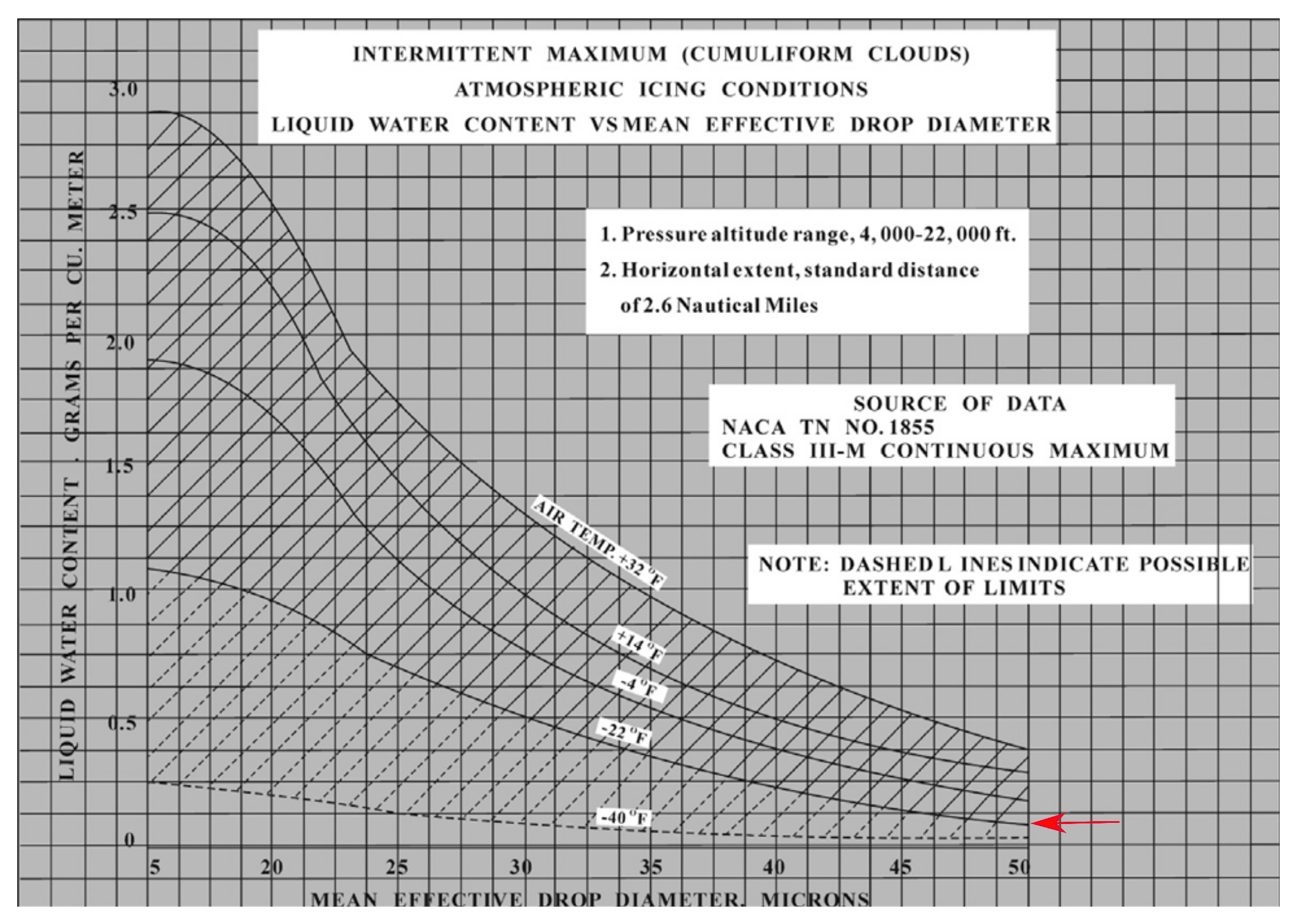
Among the parameters affect aircraft icing, the cloud type (Stratiform cloud and Cumuliform cloud) determines the liquid water content and water droplet diameter distributions [28]. In the stratiform cloud, smaller droplet diameter and lower liquid water content with larger horizontal distribution area often occur. FAR-25 [15] defines the relationship among LWC, droplet diameter and ambient temperature as shown in Figure 1. The corresponding icing condition is referred as continuous maximum icing (CMI). The water droplet diameter in the cumuliform cloud is larger than that in the stratiform cloud. Therefore, the FAR-25 defines icing condition occurring in the cumuliform cloud as intermittent maximum icing (IMI) condition. The relationship among LWC, droplet diameter and ambient temperature for IMI condition is shown in Figure 2. Hence, different meteorological variables (LWC, droplet diameter) can be extracted from Figure 1 and Figure 2 to further study how these factors affect the icing severity level. Additionally, different cloud sizes lead directly to different exposure time. The severity and extent of aircraft icing are positively correlated with the exposure time. Therefore, multiple exposure time are assigned to the extracted meteorological variables (LWC, droplet diameter) to study the effect of exposure time on aircraft icing severity.
The NACA0012 airfoil is studied in this paper. The flow conditions correspond to those of the experiment test case of Shin et al. [33], namely the angle of attack is , the free stream velocity is m/s, the pressure is = 101,300 pa. The static temperature K. The selected LWC, droplet diameter and exposure time are applied for the icing severity calculation.
3. Data-Driven Methods
The second part of the study made use of machine learning models for icing severity prediction. In order to predict the aircraft icing severity precisely, we firstly predict the icing severity level (Table 1) based on icing thickness described by Cao et al. [28] Aviation meteorologists could issue forecasts of meteorological variables, but the pilots would have to interpret the forecasts into an icing hazard for their own situation. Instead, the pilots would have a good idea how hazardous the icing is if they can get the icing severity level in report [1]. Besides the icing severity level, the machine learning models are also trained to predict the size of the area on the airfoil covered by ice and maximum ice thickness. Four categories are introduced in Table 1 to describe the icing severity levels. It is reasonable to consider the ice maximum thickness rather than the rate of accretion in determining the icing severity levels. Indeed, the ice thickness depends on the environmental conditions as well as the time spent in such conditions. The flight performance will not be greatly affected if the airplane does not stay for long in icing state even if the icing condition is severe.
3.1. The Extreme Gradient Boosting Model
XGBoost is a decision tree based method. It is a supervised machine learning algorithm for structured or tabular datasets on classication and regression predictive modeling problems. A detailed explanation of the computational methods of XGBoost [21] is beyond the scope of the current study. A brief introduction and generalized algorithm are presented.
Boosting is an ensemble technique where new models are added to correct the errors made by existing models. Models are added sequentially until no further improvements can be made. XGBoost is an improved Gradient Boosting algorithm where new models are created that predict the residuals or errors of prior models and then added together to make the final prediction [21]. It is called gradient boosting because it uses a gradient descent algorithm to minimize the loss when adding new models.
As an improvement, XGBoost adds the regularization factor to the loss function to represent the complexity of the trees, and it defines the objective function of the optimization in the training model, which is given by
where the is the model parameter trained from given data, L is the training loss function, such as square loss or logistic loss, which represents the matching degree between the model and the given training data. is the regularization term, such as norm or norm, which represents the complexity of the model. XGBoost uses the tree model complexity as a regularization term in the objective function to avoid overfitting [23]. A tree ensemble model predicts the output by averaging K trees.
where F is the space of regression trees. To learn the set of function in the model, we minimize the following regularized objective.
where l is a differentiable convex loss function that measures the difference between the prediction and the target . n is the number of predictions and the second term penalizes the complexity of the model. For a given tree ensemble model, the complexity of the model can be defined as
where the and are both regularization factors. is the complexity of the each leaf which is used to control tree node splitting. The node will split when the loss function is larger than the value of . is a parameter to scale the penalty, T is the number of leaves in a decision tree and is the weight of the leaf nodes. The XGBoost algorithm apply the second-order Taylor expansion to the loss function in the optimization process. Therefore, the objective function at step t can be derived as
where and are the first and second derivative of the loss function. We can also express the derivatives by the sum for each leaf node as and where represents all the data samples in leaf node j. Therefore, we can express the objective function as
The XGBoost algorithm involves the creation and addition of decision trees sequentially, each constructed based on the information from all previously built trees. Shallow trees often yield poor performance because they capture few details of the problem and are generally referred to as weak learners. Deeper trees might capture too many details of the problem and overfit the training dataset, limiting the ability to make good predictions on new data. Thus, it is important to tune the number and size of decision trees with XGBoost. Additionally, the hyperparameter learning rate also needs to be tuned to prevent the model from quickly fitting and then overfitting the training dataset. It scales the newly added weights to reduce the influence of each individual tree and leaves space for future trees to improve the model. In the current work, we firstly selected multiple combinations of the three parameters within reasonable ranges. For the number of trees, we evaluated a series of values from 600 to 1200 with a step size of 100 for the regression model and from 50 to 350 with a step size of 50 for the classification model. Four different values of the size of trees are selected. The learning rate is varied on a scale from to . Then, the cross-validation is performed on the training dataset with different parameter combinations and the one produces the minimum mean square error on the validation dataset is selected and used in the final models.
3.2. Data Sets
Data preparation is the first step to build the predictive model. In the current work, the models were trained, validated and tested on a data base of 1736 samples, consisting of high fidelity simulation data (DDES) and RANS results. The RANS data, obtained by applying the ice accretion modeling solver developed by the author in the previous work [12], are used to constitute the major part (around ) of the database. The DDES data are mainly used for comparison purpose when evaluating the model’s capability in predicting the icing severity results. The DDES results are obtained by applying the author’s newly developed icing solver [25] and described in the next section. 217 sets of meteorological variables (LWC, droplet diameter) are selected from their distribution profile at shown in Figure 1 and Figure 2 to represent a variety of icing conditions. The range of variation for LWC is from 0.04 g/m3 to 0.2 g/m3 in CMI condition and from 0.1 g/m3 to 1.07 g/m3 in IMI condition. The range of variation for droplet diameter is from 15 m to 40 m in CMI condition and from 5 m to 50 m in IMI condition. Eight exposure time are selected from 1 min to 30 min (1, 3, 6, 10, 15, 20, 25, 30 min) and then assigned to each pair of LWC and droplet diameter. The number of training samples is decided by exploring the effect of the size of training datasets on the prediction errors. The model’s performance for predicting icing area and maximum ice thickness at training datasets with different sizes are summarized in Table 2 and Table 3. From the set of full generated samples, 1215 samples are selected for the training and 521 samples for the testing. Since testing and training samples are partitioned randomly from the set of generated samples following same design principle, the testing and training data sets have the same population distribution.
3.3. Error Analysis
To evaluate the performance of the developed models to predict the icing area and maximum ice thickness, multiple error analysis measures were performed. For predicting the icing severity level, the model’s performance evaluation is introduced in the next section.
3.3.1. RMSE
The root mean squared error (RMSE) was calculated for the regression model. It presents an estimate of by how much each predicted outcome will deviate from its true value.
3.3.2.
The or Coefficient of determination is another measure for the regression model which presents how well the model can replicate the true outcomes. Sufficient agreement is achieved when [23].
where is the mean of the true outcomes.
3.3.3. Distribution of Errors
The errors are calculated as fractions given by the value of residuals divided by the true outcomes. The histograms are constructed to examine the nature of the error distributions. It is the most informative measure of prediction model performance.
4. Simulations and Results
4.1. Numerical Simulation Results
For the DDES computation, the baseline topology of the grid is a C-type structured grid as shown in Figure 3. The far-field boundaries are located 50 chord lengths (c) away from the airfoil to diminish the influence of the boundary condition and the spanwise domain size is . The first layer heights is . The grid details are presented in Table 4, in which , , and are the numbers of grid points along the circumference direction, the wall-normal direction, and the spanwise direction, respectively, and the represents the number of grid points on the airfoil surface. Since the main focus of the current work is the development of the icing severity prediction model, the instantaneous flow field will not be discussed in this paper.
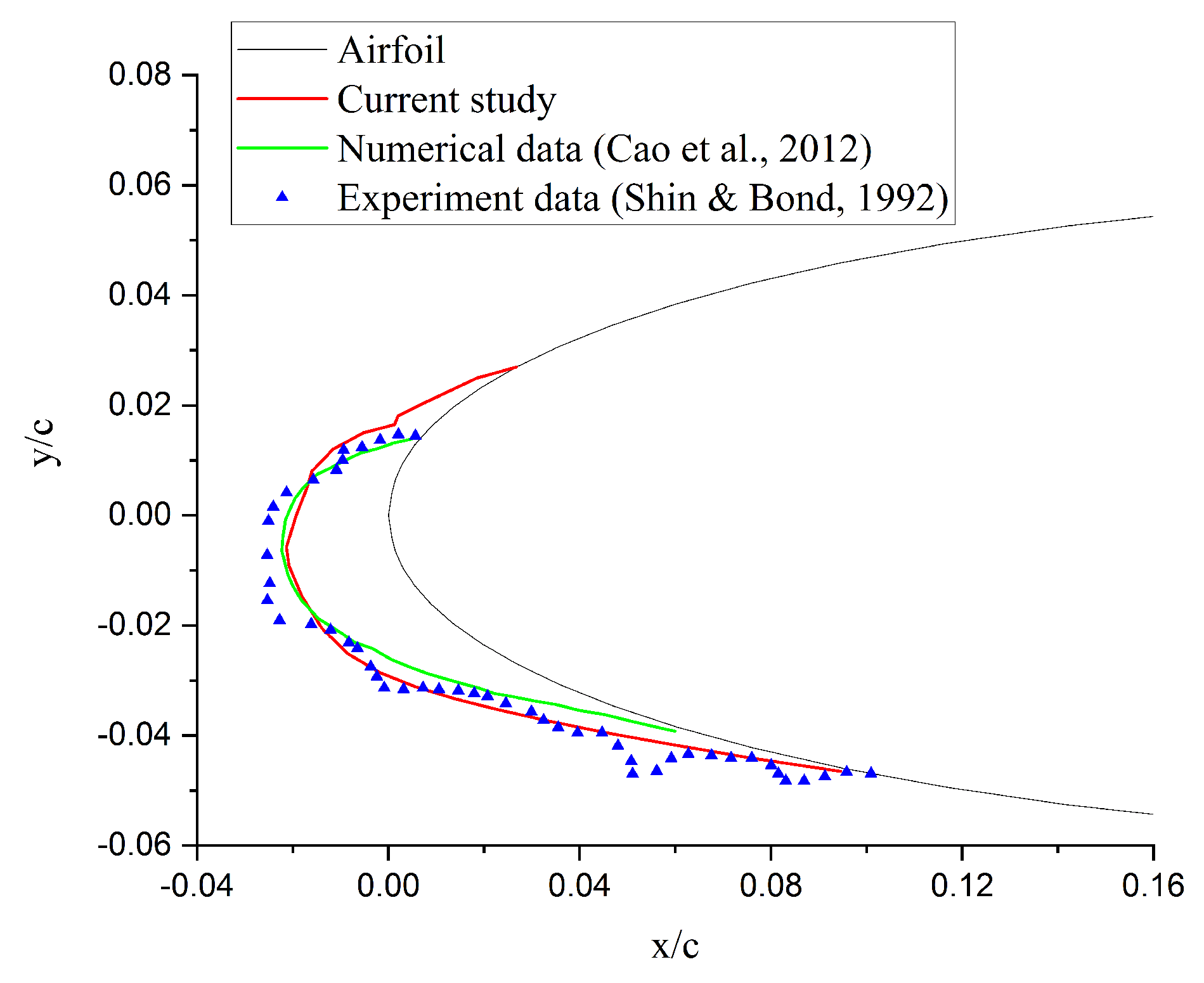
To carry out the ice accretion simulation, the meteorological factors and droplet diameter is set to be 1.0 g/m3 and 20 m, respectively. The exposure time is 360 s. For validation purposes, Figure 4 shows the ice shape comparison between the simulated results in this paper, experimental data [33], and simulated results from Cao et al. [10]. From the comparison plot, a good agreement is obtained. It can be seen that the ice height is higher in the lower region of the airfoil. This is because the airfoil is at angles of attack, the main impingement region is at the lower surface.
4.2. Aircraft Icing Severity Evaluation Based on XGBoost
In this section, the building process of the aircraft icing severity evaluation model is described, and then the prediction results are studied and error analysis are conducted to demonstrate the effectiveness of the proposed approach. Three icing conditions, that is, LWC, droplet diameter and exposure time are given to the model. We consider three icing severity features to demonstrate the applicability of the model: icing area, maximum ice thickness and icing severity level, and then the effects of the icing conditions on the three icing severity features are studied. Chang et al. [35] suggest that using both the separated-specimen method and the whole-set method to conduct the simulation to comprehensively evaluate the model’s performance. The separated-specimen method is used to divide the database into the CMI condition and the IMI condition. For each feature, we explore the effect of training dataset type on the model performance by carrying out the prediction for each dataset. A schematic of the proposed workflow is shown in Figure 5.
4.2.1. Icing Area and Maximum Ice Thickness Evaluation
In this case, the model is used to predict the area size covered by ice and the maximum ice thickness on the airfoil. The performance of the model is summarized in Table 5 and Table 6 for the three datasets: CMI dataset, IMI dataset and the whole dataset. It can be observed that the larger training set yields lower prediction errors. More importantly, the fact that the model yields the best performance on the whole dataset indicates that the model is capable of differentiating the CMI and IMI condition when evaluating the icing area and maximum ice thickness. The CPU time is recorded as the training time. The tests are performed on the 3.5 GHz Intel Core i7 processor in serial.
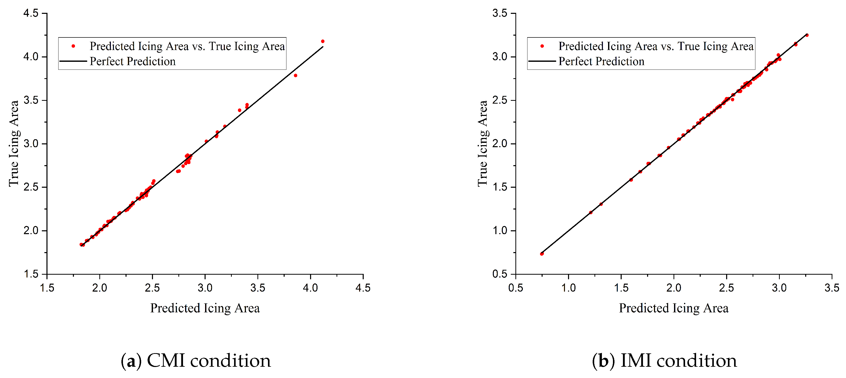
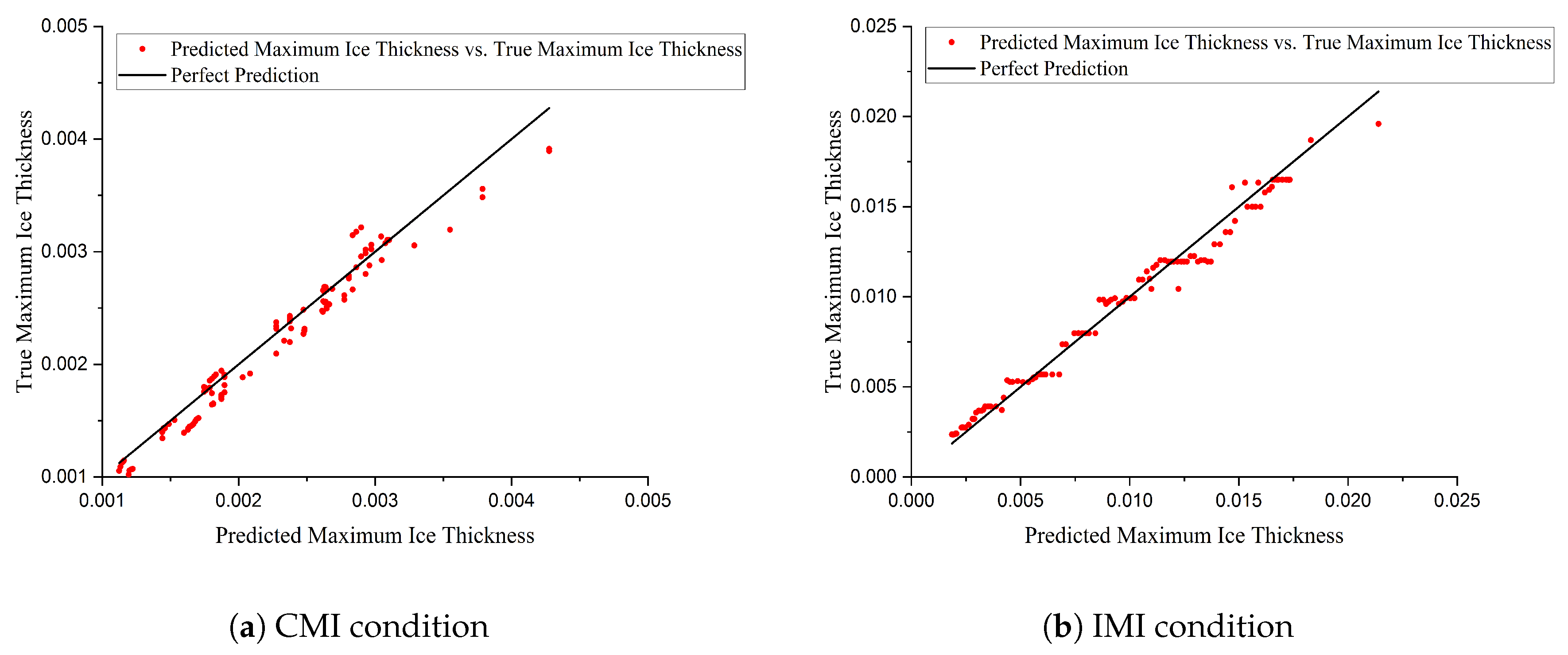
To further demonstrate the effectiveness of the model, we present the comparison between the true results and predicted results in the test dataset in Figure 6 and Figure 7. The scatter plot is the true icing area versus the predicted icing area and true maximum ice thickness versus the predicted maximum ice thickness, and the black line with unit slope represents a perfect prediction. They indicate that the sufficient agreement is achieved between the predicted and true result.
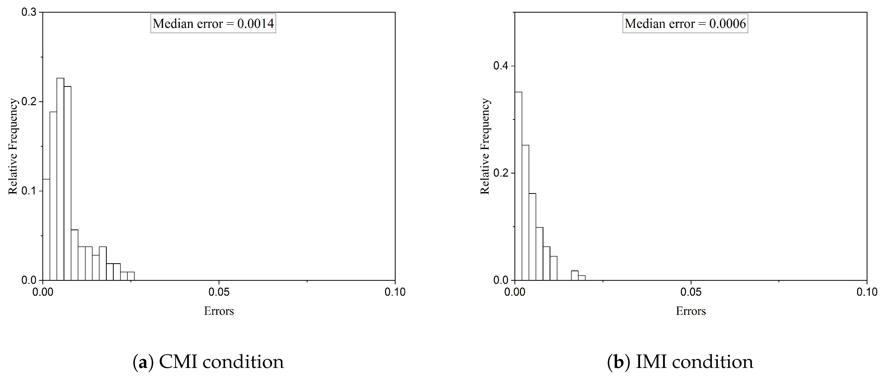
The Figure 8 and Figure 9 present the histograms of the test errors to examine the nature of the error distributions. For predicting the icing area, the median error is 0.0014 in CMI condition and 0.0006 in IMI condition. For predicting maximum ice thickness, the median error is 0.0420 in CMI condition and 0.0400 in IMI condition. All of them are lower than 0.0500, which is deemed satisfactory [23].
Figure 10 presents the recreated icing area and maximum ice thickness corresponding to the LWC and droplet diameter distribution shown in Figure 1 and Figure 2 using the predictive model. It can be observed that in both conditions, the model’s results have good agreement with the DDES results. In the CMI condition, the RANS method tends to underpredict the icing area and the maximum ice thickness as well. Since the model is trained on the datasets comprises not only RANS data but DDES data as well, the model is able to learn an average result. The IMI condition represents the icing condition occurring in the cumuliform clouds which is generally unstable relative to the stratiform clouds. Furthermore, due to the complexity and unsteadiness of the ice accretion process itself, indeed, the icing results shown in Figure 10b shows more strong oscillations. However, it should be noted that the icing area and maximum ice thickness oscillates strongly but with little changes for small droplets (less than 15 m). Those small droplets do not contribute much to icing. Overall, it can be concluded that fairly good agreement is achieved for the model.
In both conditions, the larger the water droplets, the thicker the ice layer, the greater impact on the aircraft safety. By comparing Figure 10a,b, we can notice that in general, the maximum ice thickness in IMI condition is higher than it is in CMI condition. This is because that CMI condition represents the occurrence of icing in Stratiform cloud which usually has lower liquid water content than cumuliform cloud. The LWC represents the amount of supercooled water droplets that an aircraft can hit in a given air mass, thus, the thickness of ice increases with the increase of LWC and cause greater damage to the aerodynamic performance.
Figure 11 shows the effect of exposure time on the icing area with the median value of LWC and droplet diameter. The predicted icing area and the DDES results are in good agreement. As expected, in both conditions, the icing area increases with the increase of exposure time. It should be noticed that the icing area growth ratio are increasing with time, which means that the longer a flight stays in the icing cloud, the faster the icing area increases. This observation might be attributed to the runback water effect [11]. The conductive heat transfer plays a dominant role in the ice accretion process, thus, it can be fairly assumed that in the early icing stage where very thin ice layer created, all the water droplets gets frozen immediately upon the impact on the aircraft surface and there exists no overflow water. The conductive heat loss gets weaker as the ice layer thickness increases and the overflow water first appears as the ice layer has grown to a certain extent which is referred to as critical ice thickness [11]. Since the overflow water is mainly driven by the air/water interface friction, it moves closely follows the wall air streamlines [36]. Hence, it is appropriate to consider that the overflow water might contribute to the icing area increment.
Figure 12 shows that the built model can successfully capture the maximum ice thickness with exposure time with the median value of LWC and droplet diameter. Intuitively, the longer the aircraft stays in icing condition, the thicker the ice layer, which is also confirmed by Figure 12. Additionally, it is worth mentioning that thickness growth ratio is decreasing with time. Again, it can be accounted for by the runback water effect. As the ice layer grows to the critical ice thickness, only part of the water droplet gets frozen, which slows down the maximum ice thickness growing speed.
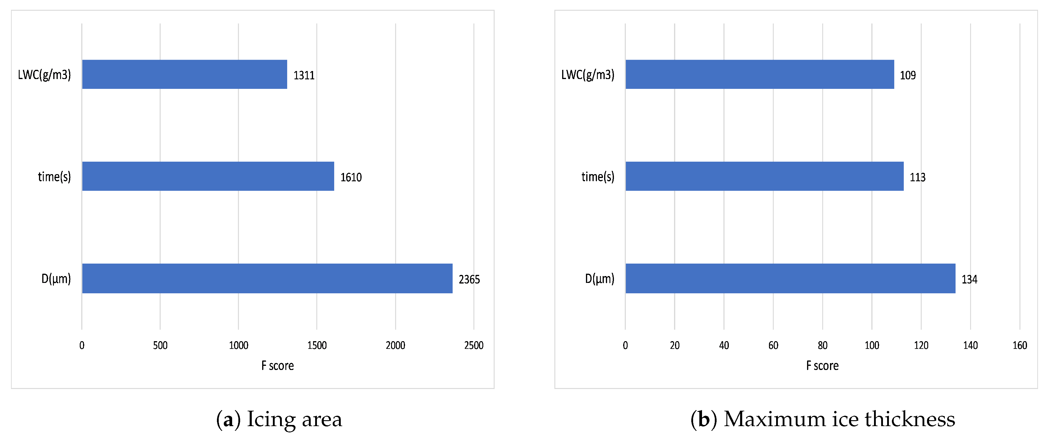
A benefit of using ensembles of decision tree methods like XGBoost is that they can provide estimates of feature importance from a trained predictive model. Generally, scores are generated to indicate how useful or valuable each feature was in the construction of the boosted decision trees within the model. In this case, we output the feature importance to rank the importance of the three input parameters to the icing severity results. The scores are summarized in the Figure 13 where D represents the droplet diameter. We can see that the droplet diameter has the highest importance and the LWC has the lowest importance with regards to icing area. In terms of maximum ice thickness, droplet diameter has the highest importance, the exposure time and LWC have a comparable level of importance.
4.2.2. Icing Severity Level Determination
For predicting the icing severity levels, the model is quantitatively evaluated by using several model evaluation indicators, such as precision, recall rate, F1 score and confusion matrix. The binary classification problem is taken as an example to explain the definitions of these measures. For each icing severity level prediction, the dataset are divided into true positive (TP), false positive (FP), true negative (TN) and false negative (FN) according to the combination of its real category and machine learning model prediction category.
- PrecisionPrecision indicates the proportion of the positive prediction which was correct. It is defined as the number of true positives (TP) over the number of true positives plus the number of false positives (FP).
- Recall RateRecall Rate indicates the proportion of actual positives was identified correctly. It is defined as the number of true positives (TP) over the number of true positives plus the number of false negatives (FN).
- F1 ScoreF1 Score relates precision and recall and is defined as the harmonic mean of them.
- Confusion MatrixThe confusion matrix [37] is used for evaluating the model when faced with a multi-classification problem. In the current work, it is applied to measure the performance of the model predicting the icing severity level. Each row of the matrix represents the predicted category while each column represents the actual category, which allows more detailed analysis than mere proportion of correct classifications.
The above mentioned evaluation indicators are summarized in Table 7. It can be seen that in the confusion matrix, the diagonal values are much higher than the non-diagonal value. The precision and recall rate for the four categories are all above . It shows that the XGBoost model has high accuracy when predicting icing severity level. It should be noticed that there are three extreme error cases: two severe predictions instead of light and one light prediction instead of severe. By looking into the error samples, the two severe predictions happens at 30 min exposure time. The corresponding LWC and droplet diameter indicate the icing severity level should be light though. The light prediction happens at 15 min exposure time. The feature importance shown in Figure 14 indicates that the model put much more weight on exposure time than LWC. Thus, the wrong severe prediction might be caused by the large exposure time.
The feature importance is reported in Figure 14, from which we can see that the droplet diameter and the exposure time have the highest importance and the LWC has the lowest importance with regards to icing severity level prediction. The noticeable difference between Figure 13b and Figure 14 might be attributed to model’s training process. Although the maximum ice thickness and the icing severity level have the similar physical meaning, the model might adopt different weights during the training process to generate the satisfied results for continuous variable and ordinal variable.
5. Conclusions
In this study, we proposed an approach to provide quick evaluations of aircraft icing severity at different flight conditions based on the machine learning model XGBoost. In its application to predict icing area, maximum ice thickness and icing severity level, well-defined performance measures are carried out through the training and testing process. It was found that the new method shows promising performance in different types of icing conditions. Due to its small computational resources requirement, fast performance and reasonable accuracy, the new method can provide an attractive alternative to traditional numerical simulation approach. Additionally, its ability to generate the feature importance can help to study the effect of different aerodynamic and meteorological factors on the icing severity results. The limitation found on the use of the current method is that the range of predictions is limited to the input data range. For example, it will not be able to predict icing severity precisely for different wings.
The proposed method has the potential to be coupled with other ice protection systems to further increase the flight safety. Additionally, coupling the proposed method with other computational fluid dynamics codes to estimate the degradation of the aircraft performance is currently being explored. If successful, a short-term application of this study would be to use the trained model to obtain a more comprehensive ‘off-line’ mapping of ice severity that incorporates a larger data-set of meteorological data and flight conditions. A long term application would be to use the trained model in a on-board software to help the pilot determine ‘on-line’ the severity as function of current conditions.
Author Contributions
Conceptualization, S.L., M.H. and R.P.; methodology, S.L., M.H.; software, J.Q.; validation, J.Q. and S.L.; formal analysis, S.L. and R.P.; investigation, S.L. and R.P.; resources, R.P.; writing—original draft preparation, S.L.; writing—review and editing, R.P.; visualization, S.L.; supervision, R.P.; funding acquisition, R.P. All authors have read and agreed to the published version of the manuscript.
Funding
This work was supported by Argonne National Laboratory through grant #ANL 4J-30361-0030A to R. Paoli and titled “Multiscale modeling of complex flows”.
Acknowledgments
The authors would like to acknowledge the constructive comments, and suggestions provided by the anonymous reviewers that greatly improved the quality of the article.
Conflicts of Interest
The authors declare no conflict of interest.
References
- McCann, D.W. NNICE—A neural network aircraft icing algorithm. Environ. Model. Softw. 2005, 20, 1335–1342. [Google Scholar] [CrossRef]
- Bragg, M.B.; Broeren, A.P.; Blumenthal, L.A. Iced-airfoil aerodynamics. Prog. Aerosp. Sci. 2005, 41, 323–362. [Google Scholar] [CrossRef]
- Ratvasky, T.P.; Ranaudo, R.J. Icing Effects on Aircraft Stability and Control Determined from Flight Data, Preliminary Results. In Proceedings of the 31st Aerospace Sciences Meeting, Reno, NV, USA, 11–14 January 1993. [Google Scholar]
- Messinger, B.L. Equilibrium temperature of an unheated icing surface as a function of air speed. J. Aeronaut. Sci. 1953, 20, 29–42. [Google Scholar] [CrossRef]
- Myers, T.G. Extension to the Messinger Model for Aircraft Icing. AIAA J. 2001, 39, 211–221. [Google Scholar] [CrossRef] [Green Version]
- Ruff, G.; Berkowitz, B. User’s Manual for the NASA Lewis Ice Accretion Prediction Code (LEWICE); NASA-CR-185129; NASA: Washington, DC, USA, 1990.
- Wright, W.B. User Manual for the NASA Glenn Ice Accretion Code LEWICE, Ver. 2.2.2; NASA/CR-2002-211793; NASA: Washington, DC, USA, 2002.
- Gori, G.; Zocca, M.; Garabelli, M.; Guardone, A.; Quaranta, G. PoliMIce: A simulation framework for three-dimensional ice accretion. Appl. Math. Comput. 2015, 267, 96–107. [Google Scholar] [CrossRef]
- Pena, D.; Hoarau, Y.; Laurendeau, E. A single step ice accretion model using Level-Set method. J. Fluids Struct. 2016, 65, 278–294. [Google Scholar] [CrossRef] [Green Version]
- Cao, Y.; Ma, C.; Zhang, Q.; Sheridan, J. Numerical simulation of ice accretions on an aircraft wing. Aerosp. Sci. Technol. 2012, 23, 296–304. [Google Scholar] [CrossRef]
- Cao, Y.; Huang, J.; Yin, J. Numerical simulation of three-dimensional ice accretion on an aircraft wing. Int. J. Heat Mass Transf. 2016, 92, 34–54. [Google Scholar] [CrossRef]
- Li, S.; Paoli, R. Modeling of Ice Accretion over Aircraft Wings Using a Compressible OpenFOAM Solver. Int. J. Aerosp. Eng. 2019, 2019, 11. [Google Scholar] [CrossRef]
- Weller, H.G.; Tabor, G.; Jasak, H.; Fureby, C. A tensorial approach to computational continuum mechanics using object-oriented techniques. Comput. Phys. 1998, 12, 620–631. [Google Scholar] [CrossRef]
- Lampton, A.; Valasek, J. Prediction of Icing Effects on the Dynamic Response of Light Airplanes. J. Guid. Control Dyn. 2007, 30, 722–732. [Google Scholar] [CrossRef]
- F.A. Regulations, Part 25—Airworthiness Standards: Transport Category Air-Planes; Federal Aviation Administration (FAA): Washington, DC, USA, 2013.
- Ogretim, E.; Huebsch, W.; Shinn, A. Aircraft Ice Accretion Prediction Based on Neural Networks. J. Aircr. 2006, 43, 233–240. [Google Scholar] [CrossRef]
- Cao, Y.; Yuan, K.; Li, G. Effects of ice geometry on airfoil performance using neural networks prediction. Aircr. Eng. Aerosp. Technol. 2011, 83, 266–274. [Google Scholar] [CrossRef]
- Fossati, M.; Habashi, W.G. Multiparameter analysis of aero-icing problems using proper orthogonal decomposition and multidimensional interpolation. AIAA J. 2013, 51, 946–960. [Google Scholar] [CrossRef]
- Zhan, Z.; Habashi, W.G.; Fossati, M. Real-Time Regional Jet Comprehensive Aeroicing Analysis via Reduced-Order Modeling. AIAA J. 2016, 54, 3787–3802. [Google Scholar] [CrossRef] [Green Version]
- Li, S.; Paoli, R.; D’Mello, M. Scalability of OpenFOAM Density-Based Solver with Runge–Kutta Temporal Discretization Scheme. Sci. Program. 2020, 2020, 11. [Google Scholar] [CrossRef]
- Chen, T.; Guestrin, C. XGBoost: A Scalable Tree Boosting System. In Proceedings of the 22nd ACM SIGKDD International Conference on Knowledge Discovery and Data Mining, San Francisco, CA, USA, 13–17 August 2016; ACM: New York, NY, USA, 2016; pp. 785–794. [Google Scholar]
- Friedman, J.H. Greedy function approximation: A gradient boosting machine. Ann. Stat. 2001, 29, 1189–1232. [Google Scholar] [CrossRef]
- Nwachukwu, A.; Jeong, H.; Pyrcz, M.; Lake, L.W. Fast evaluation of well placements in heterogeneous reservoir models using machine learning. J. Pet. Sci. Eng. 2018, 163, 463–475. [Google Scholar] [CrossRef]
- Zhang, D.; Qian, L.; Mao, B.; Huang, C.; Huang, B.; Si, Y. A Data-Driven Design for Fault Detection of Wind Turbines Using Random Forests and XGboost. IEEE Access 2018, 6, 21020–21031. [Google Scholar] [CrossRef]
- Li, S.; Paoli, R. Numerical Study of Ice Accretion over Aircraft Wings Using Delayed Detached Eddy Simulation. In Proceedings of the 72nd Annual Meeting of the APS Division of Fluid Dynamics, Seattle, WA, USA, 23–26 November 2019. [Google Scholar]
- Spalart, P.R.; Deck, S.; Shur, M.L.; Squires, K.D.; Strelets, M.K.; Travin, A. A New Version of Detached-eddy Simulation, Resistant to Ambiguous Grid Densities. Theor. Comput. Fluid Dyn. 2006, 20, 181. [Google Scholar] [CrossRef]
- Modesti, D.; Pirozzoli, S. A low-dissipative solver for turbulent compressible flows on unstructured meshes, with OpenFOAM implementation. Comput. Fluids 2017, 152, 14–23. [Google Scholar] [CrossRef]
- Cao, Y.; Tan, W.; Wu, Z. Aircraft icing: An ongoing threat to aviation safety. Aerosp. Sci. Technol. 2018, 75, 353–385. [Google Scholar] [CrossRef]
- Liou, M.S.; Steffen, C. A New Flux Splitting Scheme. J. Comput. Phys. 1993, 107, 23–39. [Google Scholar] [CrossRef] [Green Version]
- Spalart, P.; Allmaras, S. A one-equation turbulence model for aerodynamic flow. In Proceedings of the 30th Aerospace Sciences Meeting and Exhibit, Reno, NV, USA, 6–9 January 1992. [Google Scholar]
- Silva, G.L.D.; Pimenta, M. Proposed Wall Function Models for Heat Transfer around a Cylinder with Rough Surface in Cross Flow; SAE Technical Papers; SAE international: Warrendale, PA, USA, 2011. [Google Scholar]
- Henzeand, C.; Bragg, M. Turbulence Intensity Measurement Technique for Use in Icing Wind Tunnels. J. Aircr. 1999, 36, 577–583. [Google Scholar]
- Shin, J.W.; Bond, T.H. Experimental and computational ice shapes and resulting drag increase for a NACA 0012 airfoil. In Proceedings of the 5th Symposium on Numerical and Physical Aspects of Aerodynamic Flows, Long Beach, CA, USA, 13–15 January 1992. [Google Scholar]
- Pedregosa, F.; Varoquaux, G.; Gramfort, A.; Michel, V.; Thirion, B.; Grisel, O.; Blondel, M.; Prettenhofer, P.; Weiss, R.; Dubourg, V.; et al. Scikit-Learn: Machine Learning in Python. J. Mach. Learn. Res. 2011, 12, 2825–2830. [Google Scholar]
- Chang, S.; Leng, M.; Wu, H.; Thompson, J. Aircraft ice accretion prediction using neural network and wavelet packet transform. Aircr. Eng. Aerosp. Technol. 2016, 88, 128–136. [Google Scholar] [CrossRef]
- Cao, Y.; Huang, J.; Yin, J. ONERA three-dimensional icing model. AIAA J. 1995, 33, 1038–1045. [Google Scholar]
- Powers, D.M.W. Evaluation: From Precision, Recall and F-Factor to ROC, Informedness, Markedness & Correlation. J. Mach. Learn. Technol. 2011, 2, 37–63. [Google Scholar]
Figure 1.
FAR-25 Appendix C continuous maximum icing (CMI) conditions (liquid water content vs. mean effective drop diameter) reproduced from Ref. [28].
Figure 1.
FAR-25 Appendix C continuous maximum icing (CMI) conditions (liquid water content vs. mean effective drop diameter) reproduced from Ref. [28].

Figure 2.
FAR-25 Appendix C intermittent maximum icing (IMI) conditions (liquid water content vs. mean effective drop diameter) reproduced from Ref. [28].
Figure 2.
FAR-25 Appendix C intermittent maximum icing (IMI) conditions (liquid water content vs. mean effective drop diameter) reproduced from Ref. [28].

Figure 3.
Computational grid for NACA0012 airfoil.

Figure 4.
Ice shape comparison on NACA0012 airfoil.

Figure 5.
Workflow of the proposed algorithm.

Figure 6.
Icing area evaluation in CMI condition and IMI condition.

Figure 7.
Maximum ice thickness evaluation in CMI condition and IMI condition.

Figure 8.
Error distribution for predicting icing area in CMI condition and IMI condition.

Figure 9.
Error distribution for predicting maximum ice thickness in CMI condition and IMI condition.
Figure 9.
Error distribution for predicting maximum ice thickness in CMI condition and IMI condition.

Figure 10.
Recreated Icing area and maximum ice thickness results in CMI and IMI conditions.

Figure 11.
Effect of exposure time on icing area.

Figure 12.
Effect of exposure time on maximum ice thickness.

Figure 13.
Bar chart of XGBoost feature importance.

Figure 14.
Bar Chart of XGBoost Feature Importance.


Table 1.
Icing severity level based on icing thickness.
| Icing Severity Level | Light | Moderate | Heavy | Severe |
|---|---|---|---|---|
| Maximum thickness (mm) | 0.1–5.0 | 5.1–15 | 15.1–30 | >30 |
Table 2.
Summary of model performance for predicting icing area at different sizes of training datasets.
Table 2.
Summary of model performance for predicting icing area at different sizes of training datasets.
| No. of Training Data | RMSE | Median Error | |
|---|---|---|---|
| 300 | 0.107 | 0.927 | 0.0040 |
| 600 | 0.058 | 0.991 | 0.0021 |
| 1200 | 0.041 | 0.999 | 0.0014 |
Table 3.
Summary of model performance for predicting maximum ice thickness at different sizes of training datasets.
Table 3.
Summary of model performance for predicting maximum ice thickness at different sizes of training datasets.
| No. of Training Data | RMSE | Median Error | |
|---|---|---|---|
| 300 | 0.049 | 0.921 | 0.0720 |
| 600 | 0.027 | 0.957 | 0.0470 |
| 1200 | 0.020 | 0.969 | 0.0400 |
Table 4.
NACA0012 airfoil grid description.
| #Grid | #Points (Million) | ||||
|---|---|---|---|---|---|
| DDES Grid | 680 | 210 | 130 | 950 | 13.22 |
Table 5.
Summary of model performance for predicting icing area on three datasets.
| Dataset | RMSE | Median Error | Training Time (s) | |
|---|---|---|---|---|
| CMI dataset | 0.103 | 0.999 | 0.0014 | 0.29 |
| IMI dataset | 0.057 | 0.999 | 0.0006 | 0.57 |
| Whole dataset | 0.036 | 0.999 | 0.0012 | 0.91 |
Table 6.
Summary of model performance for predicting maximum ice thickness on three datasets.
| Dataset | RMSE | Median Error | Training Time (s) | |
|---|---|---|---|---|
| CMI dataset | 0.097 | 0.957 | 0.0420 | 0.04 |
| IMI dataset | 0.039 | 0.987 | 0.0400 | 0.15 |
| Whole dataset | 0.020 | 0.977 | 0.0400 | 0.37 |
Table 7.
Performance evaluation of the model for predicting icing severity level.
| Confusion Matrix | Precision | Recall Rate | F1 Score | |||||
|---|---|---|---|---|---|---|---|---|
| Actual | Light | Moderate | Heavy | Severe | ||||
| Predicted | ||||||||
| Light | 55 | 0 | 2 | 1 | 0.95 | 0.96 | 0.95 | |
| Moderate | 0 | 245 | 3 | 0 | 0.99 | 0.99 | 0.99 | |
| Heavy | 0 | 1 | 161 | 0 | 0.99 | 0.97 | 0.98 | |
| Severe | 2 | 0 | 0 | 51 | 0.96 | 0.98 | 0.97 | |
© 2020 by the authors. Licensee MDPI, Basel, Switzerland. This article is an open access article distributed under the terms and conditions of the Creative Commons Attribution (CC BY) license (http://creativecommons.org/licenses/by/4.0/).
Share and Cite
MDPI and ACS Style
Li, S.; Qin, J.; He, M.; Paoli, R. Fast Evaluation of Aircraft Icing Severity Using Machine Learning Based on XGBoost. Aerospace 2020, 7, 36. https://0-doi-org.brum.beds.ac.uk/10.3390/aerospace7040036
AMA Style
Li S, Qin J, He M, Paoli R. Fast Evaluation of Aircraft Icing Severity Using Machine Learning Based on XGBoost. Aerospace. 2020; 7(4):36. https://0-doi-org.brum.beds.ac.uk/10.3390/aerospace7040036
Chicago/Turabian StyleLi, Sibo, Jingkun Qin, Miao He, and Roberto Paoli. 2020. "Fast Evaluation of Aircraft Icing Severity Using Machine Learning Based on XGBoost" Aerospace 7, no. 4: 36. https://0-doi-org.brum.beds.ac.uk/10.3390/aerospace7040036
Note that from the first issue of 2016, this journal uses article numbers instead of page numbers. See further details here.