
Aircraft Flight Stabilizer System by CDM Designed Servo State-Feedback Controller

1
Graduate School of Science and Technology, Tokai University, Hiratsuka-shi, Kanagawa 259-1292, Japan
2
Department of Precision Engineering, Tokai University, Hiratsuka-shi, Kanagawa 259-1292, Japan
*
Authors to whom correspondence should be addressed.
Aerospace 2021, 8(2), 45; https://0-doi-org.brum.beds.ac.uk/10.3390/aerospace8020045
Submission received: 30 November 2020
/
Revised: 29 January 2021
/
Accepted: 3 February 2021
/
Published: 8 February 2021
(This article belongs to the Special Issue Aircraft Modeling for Design, Simulation and Control)
Abstract
:This research presents an automatic flight control system whose advantage is its ease of modification or maintenance while still effectively meeting the system’s performance requirement. This research proposes a mixed servo state-feedback system for controlling aircraft longitudinal and lateral-directional motion simultaneously based on the coefficient diagram method or CDM as the controller design methodology. The structure of this mixed servo state-feedback system is intuitive and straightforward, while CDM’s design processes are clear. Simulation results with aircraft linear and nonlinear models exhibit excellent performance in stabilizing and tracking the reference commands for both longitudinal and lateral-directional motion.
1. Introduction
Generally, the design process of an automatic flight control system starts from investigating the flight behavior or flight dynamics of an aircraft. The aircraft flight dynamics usually vary depending on the aircraft type. However, most aircraft exhibit a common behavior in flight dynamics if the primary flight control system remains the same. Typically, the flight dynamics model of a general aircraft becomes nonlinear. In the design of an automatic flight control system, complex procedures are involved when attempting to address nonlinear aspects of the flight dynamics model. For the sake of simplicity, sometimes, these nonlinear models need to be linearized. After such linearization, the original system model is divided into two linear components, namely, the longitudinal model and the lateral-directional model. If we focus on the relationship between these two models and the primary flight control system, the performance of the aircraft longitudinal model is strongly influenced by the deflection of the elevator, while the lateral-directional model is affected by the deflection of the aileron and rudder. Over the past decades, many researchers have investigated these aircraft flight models and proposed automatic aircraft flight control systems in a variety of means as well as for a variety of flight operations or flight envelopes. As related to previous works, an automatic flight control system is developed based on the new inversion model technique (using a Newton–Raphson trim algorithm) for advanced aircraft configurations with severe nonlinear characteristics [1]. The analysis in [2] emphasizes the feedback decoupling theory on the time domain and its application to roll attitude control. The attitude control is also studied in [3] where the automatic control is developed by using the method of calculating the torque driving the aircraft to a prescribed attitude. A well-known controller called the “Proportional–Integral–Derivative controller or PID controller” is presented for pitch attitude control in [4]; this research uses many different tuning methods to obtain the optimum parameter’s value of the PID. In [5], pitch attitude control analysis based on a singular perturbation approach theory dealing with the aircraft longitudinal decoupling was presented. These automatic aircraft flight control systems can be applied to either full or partial aircraft flight models.
The purpose of this research is to present another type of automatic flight control system, where the resulting system has a simple structure, and the design processes are straightforward. It is common to use a state-space model and a servo state feedback system to describe the aircraft dynamics and build an automatic flight control system. Its simple structure and flexibility are a primary advantage of this feedback system. The coefficient diagram method or CDM is the controller design theory used to obtain the servo state feedback gains. CDM is an efficient, easy-to-understand controller design theory and provides the decision-making criteria for determining system response in an explicit manner. In CDM, a coefficient diagram is used to analyze the system response. There are three essential parameters (stability index, , stability limit, , and equivalent time constant, ) established by CDM to adjust the system coefficient equations to meet the shape of the coefficient diagram’s needs. All three parameters also have discretionary criteria, but they can also be adjusted to achieve the desired system performance. The efficacy of the CDM has been verified by previous works in which a partial model of an aircraft is employed for simulation [6,7,8]. The entire structure of the automatic flight control system comprises two subsystems, that is, one for longitudinal control and another for lateral-directional control. The altitude and heading are controlled variables in these subsystems. Both subsystems have their controller gains, which are obtained from the linearized state-space model and separately designed by the CDM. We then applied the proposed automatic flight control system to the nonlinear aircraft flight dynamics model to investigate the system’s performance. The simulation results showed that the proposed automatic flight control system exhibited satisfactory performance while retaining simplicity in its design processes.
2. Aircraft Flight Dynamics
2.1. Longitudinal Dynamics
After linearization, the desired longitudinal dynamics in the state-space form are shown in Equation (1), where is a state vector, , is the input [9,10], which consists of the elevator deflection and thrust, and are the output. By using dimensional derivative notation, the longitudinal state matrix, , the longitudinal control matrix, , and the longitudinal output matrix, are given as shown in Equation (1).
2.2. Lateral-Directional Dynamics
Following the same way as in the longitudinal dynamics, the desired lateral-directional dynamics in the state-space form is shown in Equation (2), where is a state vector and is expressed as , is an input, which consists of the aileron and rudder deflection, and are output. By using dimensional derivative notation, the lateral-directional state matrix, , the lateral-directional control matrix, , and the lateral-directional output matrix, are given in Equation (2).
2.3. Integrated Dynamics
The integrated dynamics is a combination of longitudinal and lateral-directional dynamics. These dynamics have as a state vector, and as the input, These integrated dynamics are used for investigating the system performance and its state-space form as given in Equation (3).
3. Coefficient Diagram Method and Servo State-Feedback System
3.1. Coefficient Diagram Method
The coefficient diagram method or CDM is a kind of controller design theory and was first introduced by Professor Shunji Manabe [11]. From the efficient and uncomplicated CDM, there are many studies about CDM in various fields [12,13]. In addition, there is specific research using CDM in the aeronautic and aerospace field [14,15]. This controller design theory uses a diagram called the “coefficient diagram,” which provides sufficient information about the three primary characteristics of the control system (stability, response, and robustness). By consideration of the shape of the coefficient curve, the stability can be observed from the curvature, the response can be observed from the inclination, and the robustness can be observed from the variation of the shape of the curve due to plant/controller parameter variation. The characteristic polynomial of the desired automatic control system (closed-loop system) will determine the coefficient values in this curve. In CDM, this characteristic polynomial is obtained from the CDM’s characteristic polynomial. The CDM’s monic characteristic polynomial is shown in Equation (4),
where are the coefficients. CDM introduces three specific design parameters comprising stability index, , stability limit, , and equivalent time constant, and uses these three parameters in conjunction with Equation (4) to obtain the CDM’s characteristic polynomial. By tuning, these three parameters lead to the proper controller. CDM defines the criterion for tuning these parameters as follows: The stability index must satisfy the inequality, and the stability limit relates to the stability index, as shown in Equation (5).
The equivalent time constant is related to the settling time and shown in Equation (6),
However, CDM recommends the value set of the stability index known as the standard stability index, as shown in Equation (7),
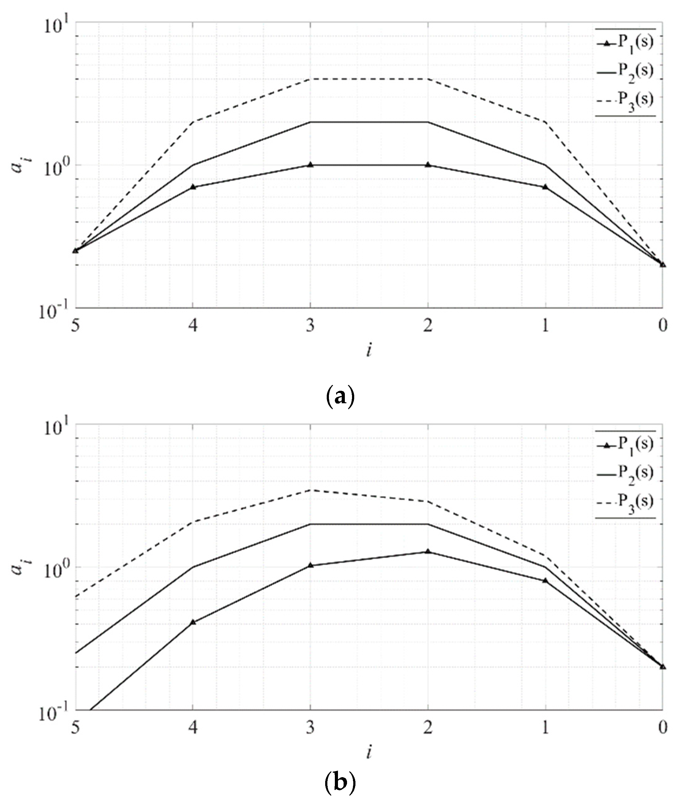
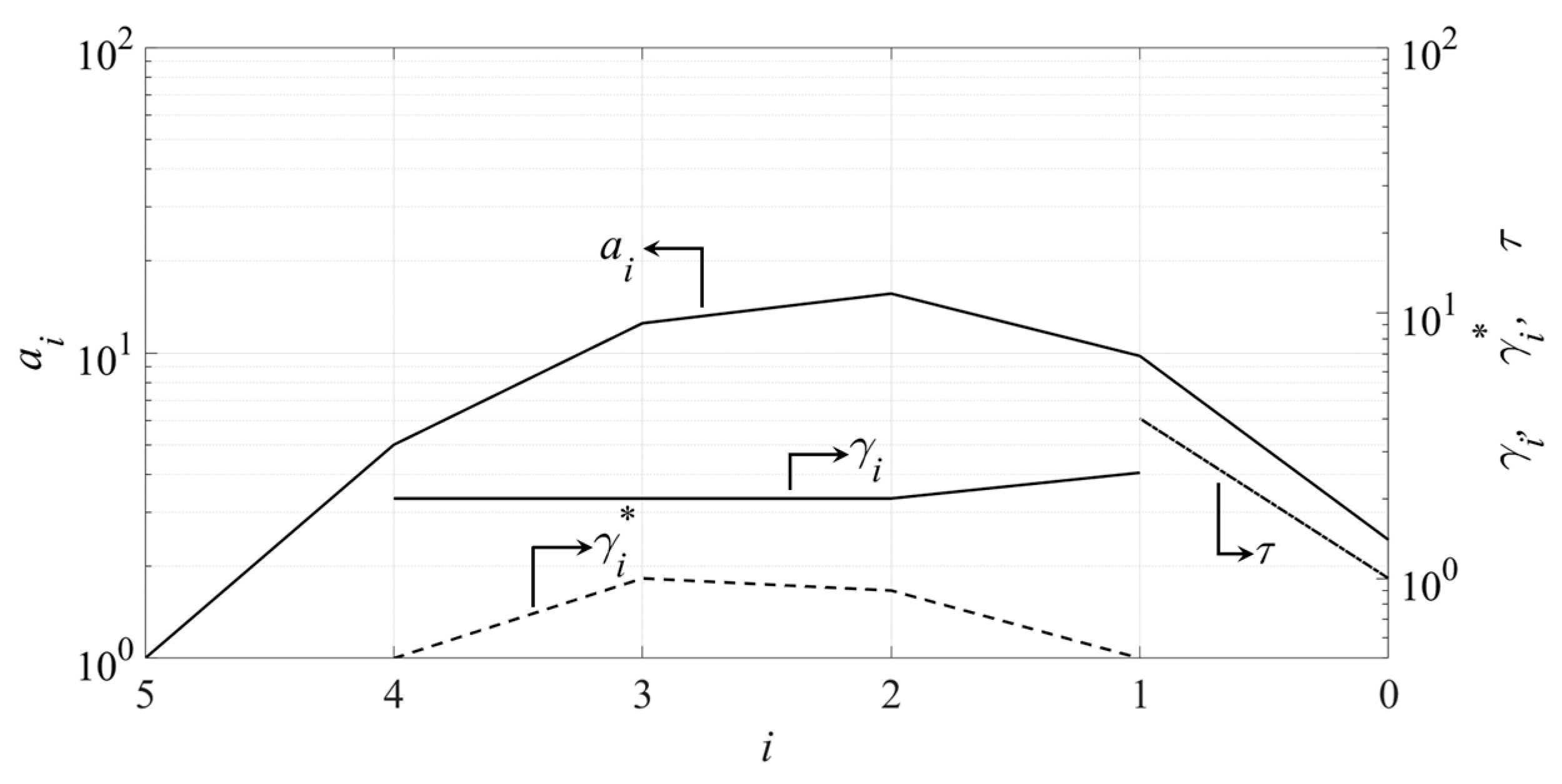
For an illustration purposes to explain how the shape of the coefficient diagram should be interpreted from a stability viewpoint, three 5th-order systems with different sets of stability index,, and the equivalent time constant,, are compared. Their characteristic polynomials and poles are expressed as Equations (8)–(10).
By considering the poles of these systems, is more stable than the other two, and the coefficient diagram of is more curved than the other, as shown in Figure 1a. For another comparison, the same stability indexes but different equivalent time constants, 4, 5, and 6, are assigned for ,, and , respectively. It is seen from Figure 1b that with the smallest equivalent time constant is more left-end down than the other two. Therefore, after observing both coefficient diagrams, the more up-lifted the diagram’s curve is, the more stable the system becomes, and the more left-end down the curve is, the faster the response becomes.
3.2. Servo State-Feedback System
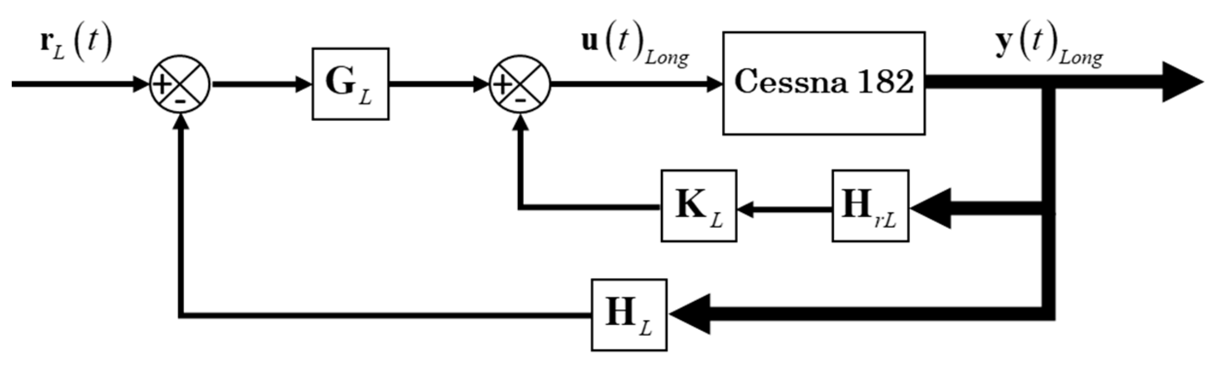
Both longitudinal and lateral-directional dynamics are the plants that have an integrator and the same pattern (same number of state variables, inputs, and outputs). Therefore, this subsection uses the longitudinal dynamics, shown in Figure 2, to explain the servo state-feedback system’s general configuration for this research [16]. In this servo system, let the output be the velocity and altitude, . Then, only three state variables remain as the variables to feedback into the system. Therefore, it is necessary to introduce two reduced matrices to complete this servo state feedback system. The reduced matrix and are shown in Equation (11).
By considering Figure 2 and Equation (1), with as the reference command, and , as state-feedback gain matrices, the input can be described as in Equation (12),
Letting be the total servo state-feedback gain matrix and using Equation (12), and , we rewrite the input again, as shown in Equation (13),
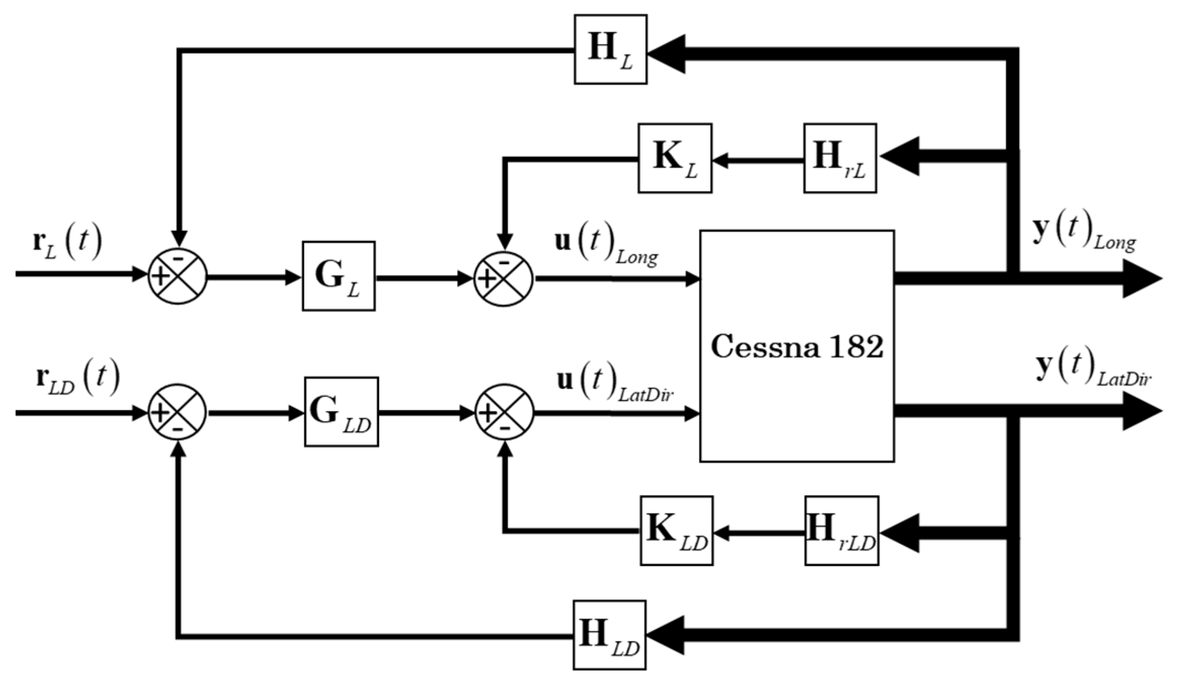
As stated previously, the lateral-directional dynamics servo state-feedback system also has two outputs (sideslip and the heading angle) and two inputs, as in the longitudinal dynamics. Therefore, we are able to apply the same configuration, as shown in Figure 2, to this system. The reduced matrices of lateral-directional dynamics servo state-feedback system, and , are identical with and , respectively. The total servo state-feedback gain matrix for both systems ( and ) is applied to the integrated dynamics, Equation (3), to obtain the proposed aircraft flight stabilizer system, as shown in Figure 3.
The aircraft flight stabilizer system in Figure 3 uses CDM to determine the total servo state-feedback gain matrix. The summary of the procedures to determine the total servo state-feedback gain matrices is given as follows.
- Choose the values of , and , to determine the desired CDM’s monic characteristic polynomial, Equation (4).
- Use the poles of obtained CDM’s monic characteristic polynomial to specify the eigenvalues of the matrix, and . Then use a pole placement technique to determine the values of the total servo state-feedback gain matrix, , and .
- Calculate the values of , for longitudinal dynamics, and , for lateral-directional dynamics.
- If necessary, the adjustment follows CDM’s criterion, Equations (5) and (6), until the system requirement can be met for each system.
4. Simulation Results
To investigate the performance of the proposed aircraft flight stabilizer system, the simulation was carried out with MATLAB® and Simulink® with Cessna 182 as the test aircraft in the linear model and nonlinear model. The nonlinear model used in this simulation was Airlib [17], developed by Giampiero Campa. This tool block was a general nonlinear 6-DOF aircraft model, with a very accurate built-in atmosphere model and constant aerodynamic derivatives. The block’s architecture was largely based on the Aircraft block provided by the FDC toolbox (Marc Rauw, 1993–2000) [18]. The geometric data of a Cessna 182 and flight condition data used in this simulation are shown in Table 1 and Table 2 [9], respectively.
The longitudinal state matrix, , the longitudinal control matrix, , the lateral-directional state matrix, and the lateral-directional control matrix, of Cessna 182 used in Equation (3) are shown in Equations (14) and (15), respectively.
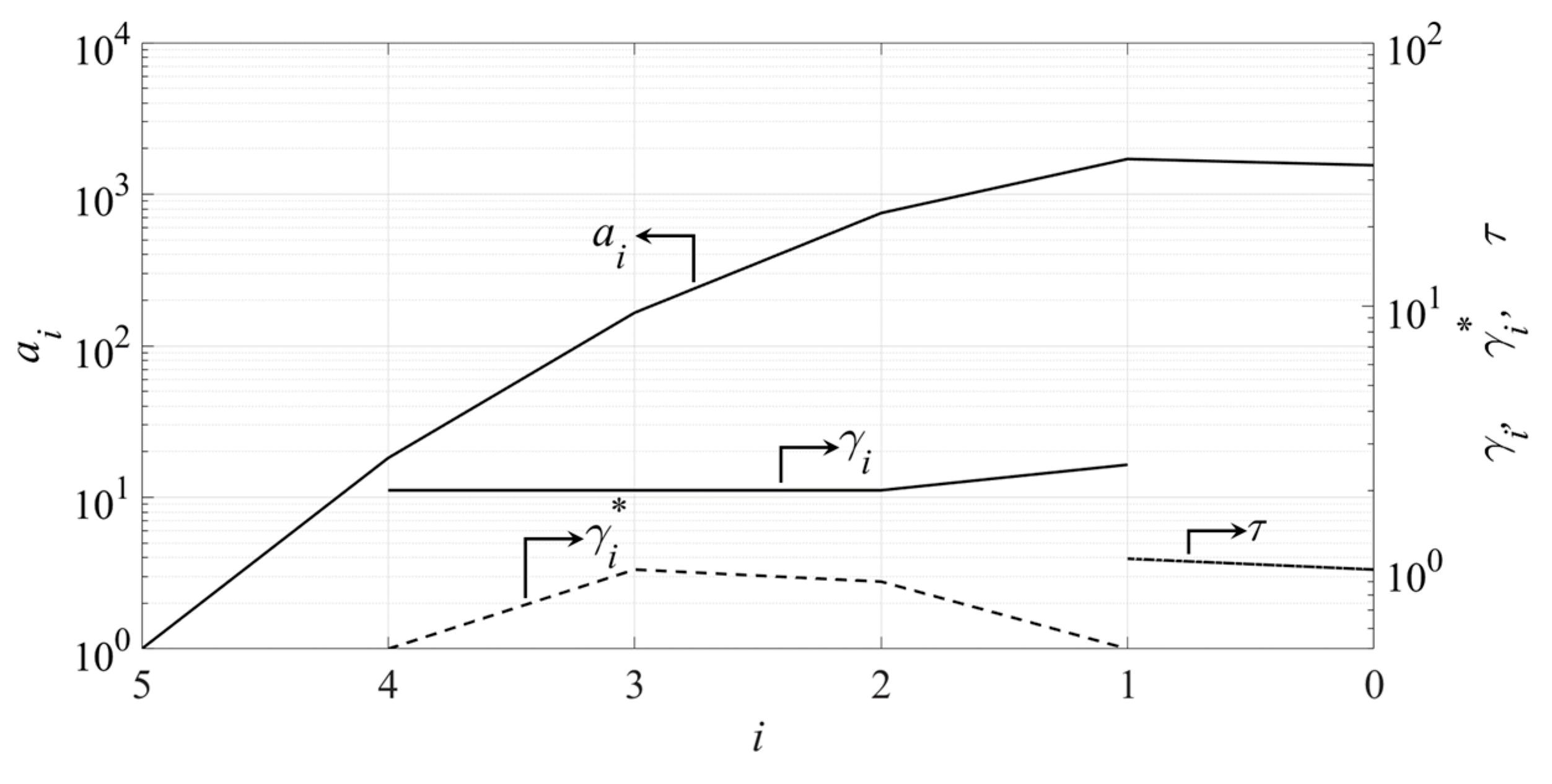
With the total servo state-feedback gain matrices obtained as above, we chose the set values of , as given in Equation (7). These set values of are called standard stability index, and CDM guarantees that the obtained system with these values has a good balance between stability, robustness, and response. The value of equal to 1.1 for longitudinal dynamics and equal to 4 for lateral-directional dynamics were chosen to meet the required system response that wants the fastest control system response as soon as possible with less overshoot. With the CDM’s monic characteristic polynomial, Equation (4), the coefficient diagrams of both subsystems are shown in Figure 4 and Figure 5.
By observing both coefficient diagrams, Figure 4 and Figure 5, both systems had stability due to the use of the same set of which can be observed from the diagram’s curvature. If the diagram’s curvature became larger, the system becomes more stable. However, the longitudinal dynamics exhibited a faster response than the lateral-directional dynamics due to a different and can be observed from the greater inclination of Figure 4 than Figure 5. The proposed control system used the obtained CDM’s polynomial to determine the total servo state-feedback gain matrices, and the controller was constructed in the Simulink®. The total servo state-feedback gain matrices for longitudinal dynamics and lateral-directional dynamics are shown in Equations (16) and (17), respectively.
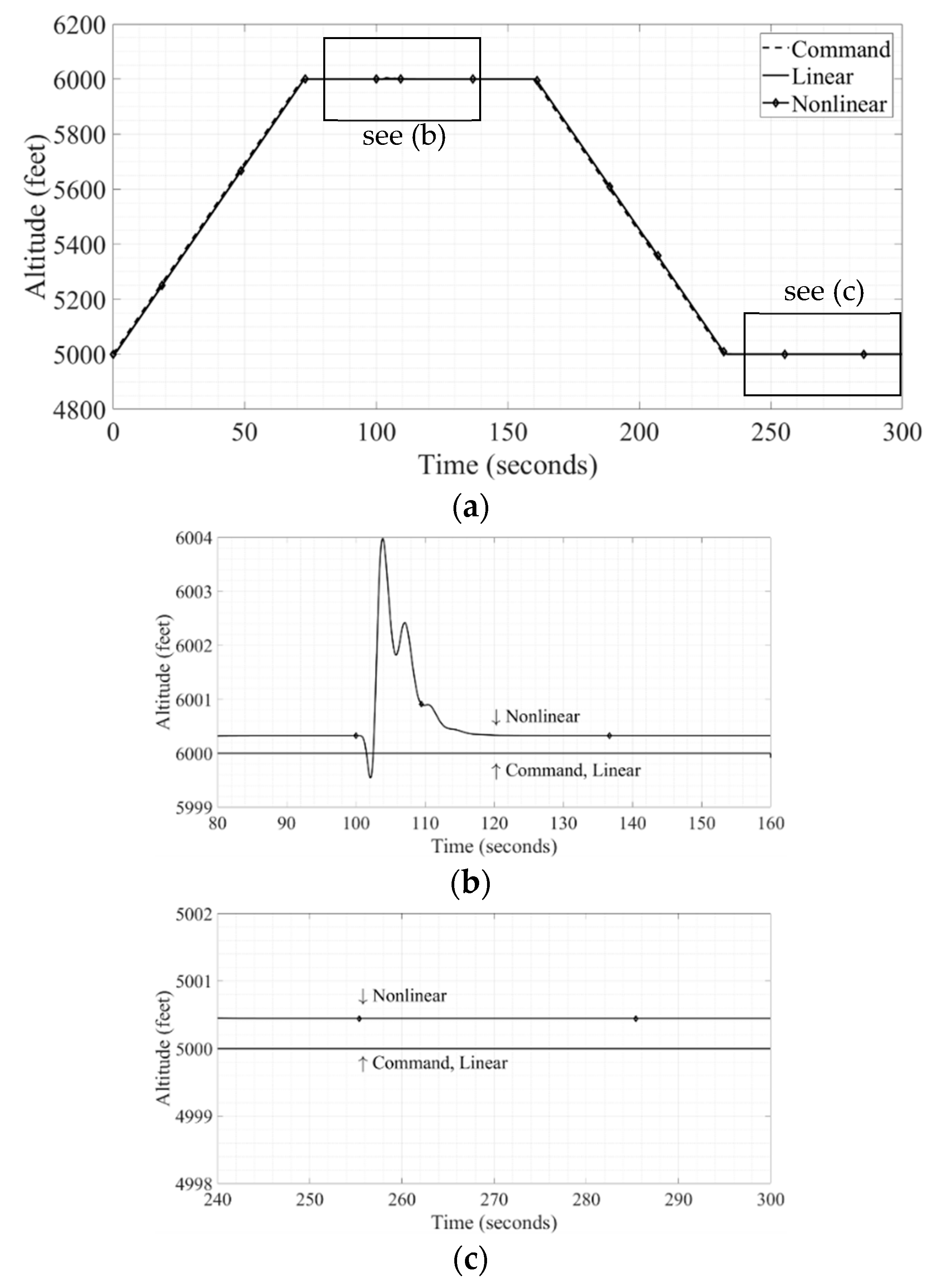
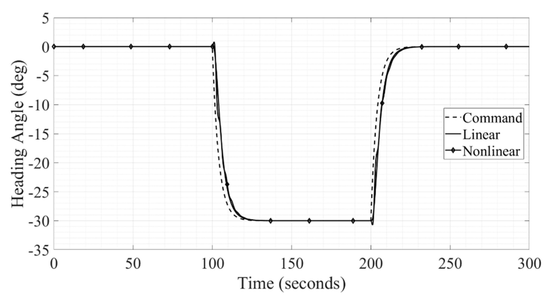
The simulation used an 840 feet per minute rate of climb and descent as a command signal to the longitudinal dynamics system and 45 degrees per minute rate of turn to the lateral-directional dynamics system. The response of altitude and heading control are shown in Figure 6 and Figure 7, respectively.
The altitude command changed from 5000 to 6000 feet at the beginning and held at this altitude until 160 s, then returned to 5000 feet. The heading command changed from 0 degrees to −30 degrees at 100 and held at this angle until 200 s, then came back to 0 degrees. The simulation response in Figure 6 illustrates that both controllers of linear and nonlinear systems exhibited excellent performance in tracking altitude command signals at the same rate of climb and descent as the command signals. However, the altitude response of the nonlinear system had a small overshoot, 0.07%, when a heading change occurred at 100 s (see Figure 6b) and had a small error, 0.01%, at a steady-state, between the command signal and response of the linear system (see Figure 6c). In the heading response (see Figure 7), both controllers of linear and nonlinear systems still exhibited excellent performance in tracking heading command signals. However, the nonlinear system’s response had a small overshoot of approximately 0.8 degrees when the heading changed. With respect to the heading command, both linear and nonlinear systems presented no steady-state error.
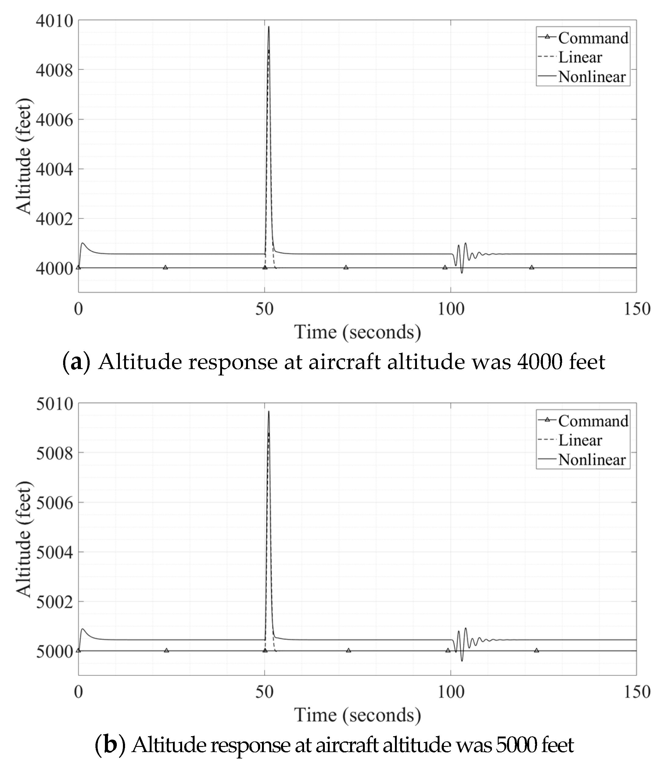
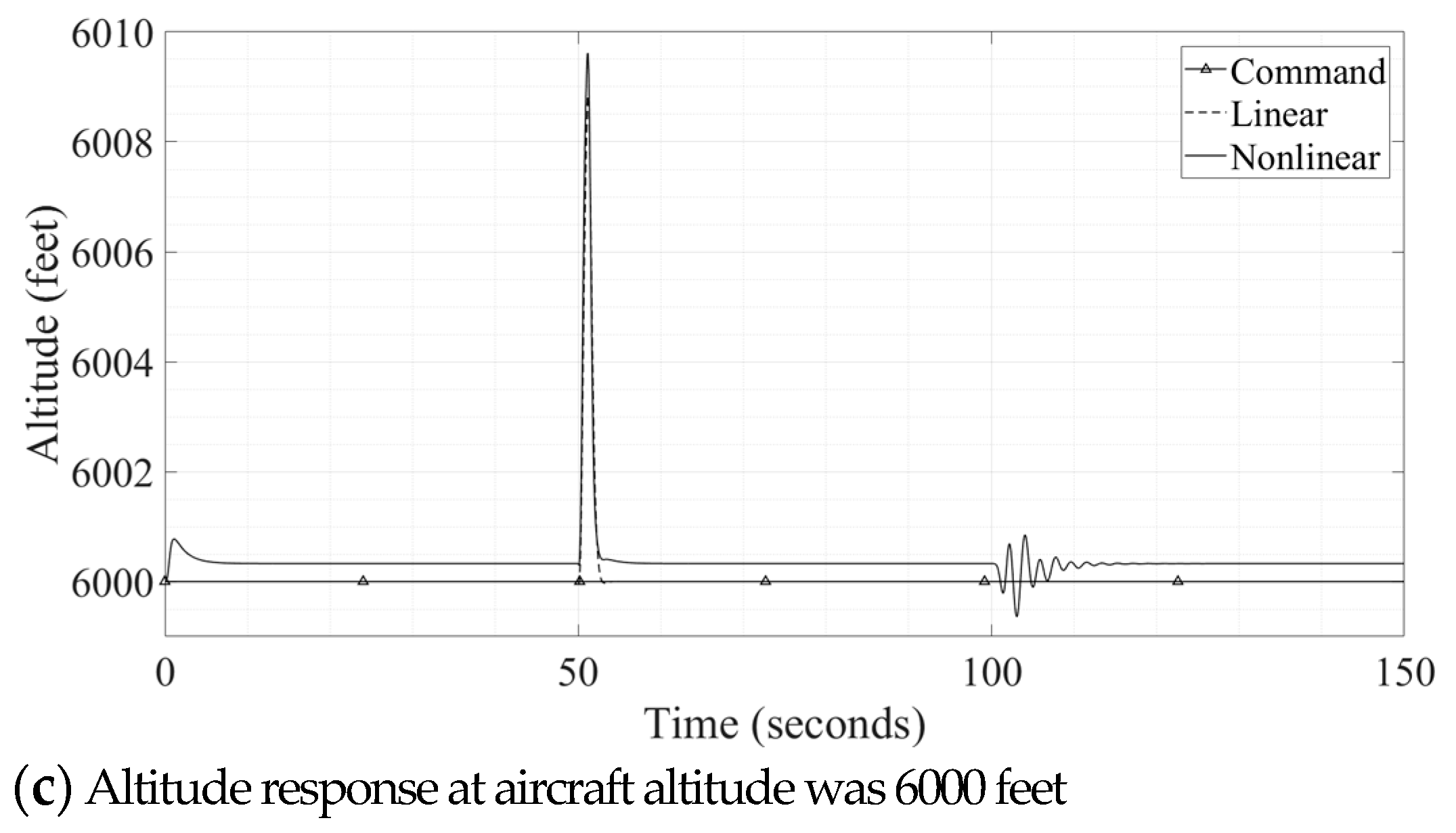
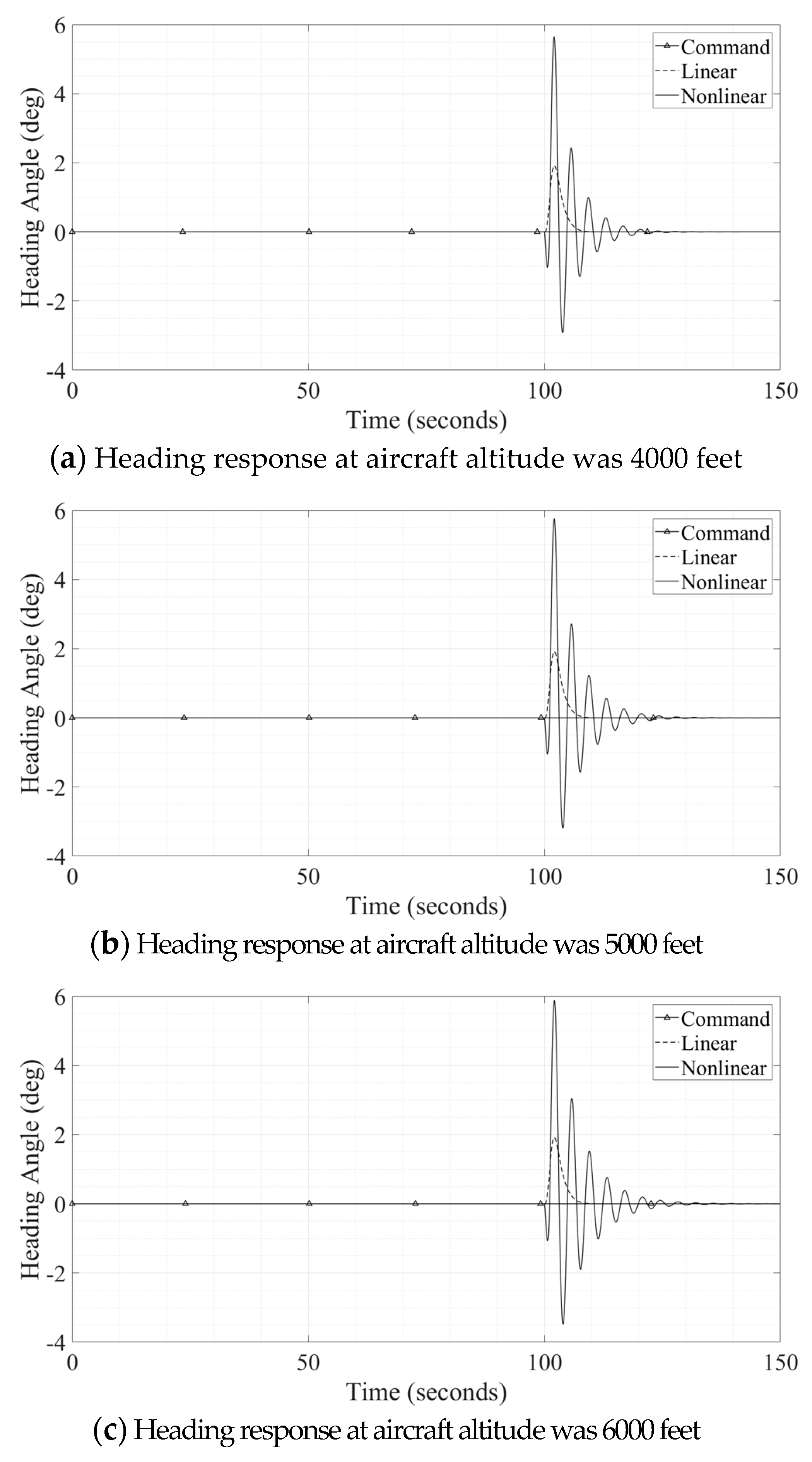
It is generally known that the aircraft’s altitude is the one crucial parameter in flight. Therefore, to investigate the proposed control system’s effectiveness, this simulation tested the control system for the aircraft’s altitude and zero-heading stabilization. There were three tested altitudes: 4000 feet, 5000 feet, and 6000 feet, and the disturbance signal to both controlled variables (altitude and heading) at each altitude test was applied. The disturbance signals were impulse signals and applied to the altitude at 50 s and heading at 100 s. The response of altitude and heading are shown in Figure 8 and Figure 9, respectively.
By observing Figure 8, it was found that the proposed control system exhibited a good disturbance rejection behavior (the disturbance signal applied directly to the altitude at 50 s) in all three tested altitudes. The proposed control system could also mitigate a change in heading occurring at 100 s. As seen in Figure 9, the heading response was not affected by the altitude change and exhibited an excellent disturbance rejection behavior (the disturbance signal applied directly to the heading at 100 s) in all three tested altitudes. Considering the proposed control system’s performance for all three flight altitude changes, the system was found to exhibit little change, which implies its robustness. For example, in Figure 8, in an attempt to maintain a constant altitude in three different levels, there was a slight change in the steady-state error when the altitude decreased. Similarly, in Figure 9, the overshoot increased only slightly as the altitude increased.
5. Conclusions
This research’s objective was to obtain an efficient controller in which the controller’s structure was straightforward and easy to modify. The consideration of the general structure of the controller, controller design processes, and the simulation results, confirmed that the obtained controller met the objectives. In terms of the controller’s structure, the use of the servo state-feedback controller, which decouples longitudinal and lateral-directional dynamics, makes these controllers easy to modify the controlled state variable for other control purposes by means of modifying the reduced matrix. Moreover, if there is a need to change the controller structure or type, it can be done partially without affecting the rest. In terms of controller design based on CDM, which is a useful and practical controller design theory, this controller design approach had a straightforward and clear criterion in tuning and guarantees that the obtained system will achieve a good balance of stability, response, and robustness.
Author Contributions
Conceptualization, E.A. and Y.Y.; validation, E.A. and Y.Y.; formal analysis, E.A.; investigation, E.A.; writing—original draft preparation, E.A. and Y.Y.; writing—review and editing, E.A. and Y.Y.; visualization, E.A. and Y.Y.; supervision, E.A. and Y.Y.; project administration, E.A. and Y.Y.; funding acquisition, Y.Y. Both authors have read and agreed to the published version of the manuscript.
Funding
This study was supported by funding of Tokai University.
Institutional Review Board Statement
Not applicable.
Informed Consent Statement
Not applicable.
Data Availability Statement
Not applicable.
Conflicts of Interest
The authors have no conflict of interest to disclose.
Nomenclature
| g | gravity acceleration, ft/sec2 |
| h | altitude, ft |
| dimensional derivative of moment | |
| p | roll angular rate, rad/sec2 |
| q | pitch angular rate, rad/sec2 |
| r | yaw angular rate, rad/sec2 |
| ts | settling time, sec |
| v | velocity, ft/sec |
| airspeed, ft/sec | |
| dimensional derivative of force | |
| angle of attack, rad | |
| sideslip angle, rad | |
| deflection of control surfaces, rad | |
| roll angle, rad | |
| stability index | |
| stability limit | |
| pitch angle, rad | |
| steady state pitch angle, rad | |
| equivalent time constant, sec | |
| yaw angle, rad | |
| Subscripts | |
| A | aileron |
| E | elevator |
| LatDir, LD | relative to the lateral-directional dynamics |
| Long, L | relative to the longitudinal dynamics |
| rL | reduce matrix of the longitudinal dynamics |
| rLD | reduce matrix of the lateral-directional dynamics |
| R | rudder |
| T | thrust |
References
- Smith, G.; Meyer, G. Aircraft Automatic Flight Control System with Model Inversion. J. Guid. 1987, 10, 269–275. [Google Scholar] [CrossRef]
- Guo, J.; Tang, S. Application of the feedback decoupling method in the attitude control of the rolling aircraft. In Proceedings of the 2012 International Conference on Systems and Informatics (ICSAI2012), Yantai, China, 19–20 May 2012; pp. 371–375. [Google Scholar]
- Zolotukhin, Y.N.; Nesterov, A.A. Aircraft attitude control. Optoelectron. Instrum. Data Process. 2015, 51, 456–461. [Google Scholar] [CrossRef]
- Deepa, S.; Sudha, G. Longitudinal control of aircraft dynamics based on optimization of PID parameters. Thermophys. Aeromech. 2016, 23, 185–194. [Google Scholar] [CrossRef]
- Shan, S.; Hou, Z.; Wang, W. Aircraft longitudinal decoupling based on a singular perturbation approach. Adv. Mech. Eng. 2017, 9, 1–8. [Google Scholar] [CrossRef]
- Asa, E.; Yamamoto, Y.; Benjanarasuth, T. Aircraft Altitude Control Based on CDM. In Proceedings of the 2019 IEEE 2nd International Conference on Information and Computer Technologies (ICICT), Kahului, HI, USA, 14–17 March 2019; Volume 14, pp. 266–269. [Google Scholar]
- Asa, E.; Yamamoto, Y. Aircraft Heading Hold Control Based on CDM. In Proceedings of the 2019 19th International Conference on Control, Automation and Systems (ICCAS), Jeju, Korea, 15–18 October 2019; pp. 247–250. [Google Scholar]
- Asa, E.; Yamamoto, Y. CDM based Controller design for Stabilizing the Altitude and Heading of an Aircraft. In Proceedings of the 2019 IEEE International Conference on Cybernetics and Intelligent Systems (CIS) and IEEE Conference on Robotics, Automation and Mechatronics (RAM), Bangkok, Thailand, 18–20 November 2019; pp. 144–148. [Google Scholar]
- Marcello, R. Aircraft Dynamics from Modeling to Simulation; John Wiley & Sons, Inc.: Hoboken, NJ, USA, 2012; Chapters 3, 4, 8; Appendix B; pp. 586–588. [Google Scholar]
- David, K. Schmidt, Modern Flight Dynamics; McGraw-Hill, Inc.: New York, NN, USA, 2012; Chapters 8, 12. [Google Scholar]
- Manabe, S. Coefficient Diagram Method. IFAC Proc. Vol. 1998, 31, 211–222. [Google Scholar] [CrossRef]
- Asa, E.; Benjanarasuth, T.; Ngamwiwit, J.; Komine, N. Hybrid controller for swinging up and stabilizing the inverted pendulum on cart. In Proceedings of the 2008 International Conference on Control, Automation and Systems, Seoul, Korea, 14–17 October 2008; pp. 2504–2507. [Google Scholar]
- Ocal, O.; Bir, A.; Tibken, B. Digital design of Coefficient Diagram Method. In Proceedings of the 2009 American Control Conference, St. Louis, MO, USA, 10–21 June 2009; Volume 10, pp. 2849–2854. [Google Scholar]
- Manabe, S. Application of Coefficient Diagram Method to Mimo Design in Aerospace. In IFAC Proceedings Volumes; Elsevier BV: Amsterdam, The Netherlands, 2002; Volume 35, pp. 43–48. [Google Scholar]
- Hirokawa, R.; Sato, K.; Manabe, S. Autopilot design for a missile with reaction-jet using coefficient diagram method. In Proceedings of the AIAA Guidance, Navigation and Control Conference and Exhibit, Montreal, QC, Canada, 6–9 August 2001. [Google Scholar]
- Ogata, K.; Brewer, J.W. Modern Control Engineering. J. Dyn. Syst. Meas. Control 1971, 93, 63. [Google Scholar] [CrossRef]
- Campa, G. Airlib, MATLAB Central File Exchange. Available online: http://www.mathworks.com/matlabcentral/fileexchange/3019-airlib (accessed on 27 January 2020).
- Rauw, M.O. FDC 1.2—A Simulink Toolbox for Flight Dynamics and Control Analysis, 2nd ed.; May 2001. Available online: http://www.dutchroll.sourceforge.net (accessed on 4 February 2020).
Figure 1.
Coefficient diagram: (a) Stability; (b) Time response.

Figure 2.
The longitudinal dynamics servo state-feedback system.

Figure 3.
Aircraft flight stabilizer system.

Figure 4.
Coefficient diagram of longitudinal dynamics.

Figure 5.
Coefficient diagram of lateral-directional dynamics.

Figure 6.
Altitude response: (a) Total response; (b) Response in 80 to 160 s; (c) Response in 240 to 300 s.
Figure 6.
Altitude response: (a) Total response; (b) Response in 80 to 160 s; (c) Response in 240 to 300 s.

Figure 7.
Heading response.

Figure 8.
Altitude response with disturbance signal at various aircraft altitude.


Figure 9.
Heading response with disturbance signal at various aircraft altitude.


Table 1.
Cessna 182 geometric data.
| Cessna 182 | Symbol | Value |
|---|---|---|
| Wing surface (ft2) | 174 | |
| MAC (ft) | 4.9 | |
| Wingspan (ft) | 36 |
Table 2.
Cessna 182 flight condition data.
| Symbol | Cruise | |
|---|---|---|
| Altitude (ft) | 5000 | |
| Mach number | 0.201 | |
| Airspeed (ft/sec) | 220.1 | |
| Dynamic Pressure (lbs/ft2) | 49.6 | |
| CG -%MAC | 0.264 | |
| AOA (deg) | 0 |
Publisher’s Note: MDPI stays neutral with regard to jurisdictional claims in published maps and institutional affiliations. |
© 2021 by the authors. Licensee MDPI, Basel, Switzerland. This article is an open access article distributed under the terms and conditions of the Creative Commons Attribution (CC BY) license (http://creativecommons.org/licenses/by/4.0/).
Share and Cite
MDPI and ACS Style
Asa, E.; Yamamoto, Y. Aircraft Flight Stabilizer System by CDM Designed Servo State-Feedback Controller. Aerospace 2021, 8, 45. https://0-doi-org.brum.beds.ac.uk/10.3390/aerospace8020045
AMA Style
Asa E, Yamamoto Y. Aircraft Flight Stabilizer System by CDM Designed Servo State-Feedback Controller. Aerospace. 2021; 8(2):45. https://0-doi-org.brum.beds.ac.uk/10.3390/aerospace8020045
Chicago/Turabian StyleAsa, Ekachai, and Yoshio Yamamoto. 2021. "Aircraft Flight Stabilizer System by CDM Designed Servo State-Feedback Controller" Aerospace 8, no. 2: 45. https://0-doi-org.brum.beds.ac.uk/10.3390/aerospace8020045
Note that from the first issue of 2016, this journal uses article numbers instead of page numbers. See further details here.