An Experimental Investigation of the Convective Heat Transfer on a Small Helicopter Rotor with Anti-Icing and De-Icing Test Setups

Abstract

Successful icing/de-icing simulations for rotorcraft require a good prediction of the convective heat transfer on the blade’s surface. Rotorcraft icing is an unwanted phenomenon that is known to cause flight cancelations, loss of rotor performance and severe vibrations that may have disastrous and deadly consequences. Following a series of experiments carried out at the Anti-icing Materials International Laboratory (AMIL), this paper provides heat transfer measurements on heated rotor blades, under both the anti-icing and de-icing modes in terms of the Nusselt Number (Nu). The objective is to develop correlations for the Nu in the presence of (1) an ice layer on the blades (Nu_Ice) and (2) liquid water content (LWC) in the freestream with no ice (Nu_Wet). For the sake of comparison, the Nu_Wet and the Nu_Ice are compared to heat transfer values in dry runs (Nu_Dry). Measurements are reported on the nose of the blade-leading edge, for three rotor speeds (Ω) = 500, 900 and 1000 RPM; a pitch angle (θ) = 6°; and three different radial positions (r/R), r/R = 0.6, 0.75 and 0.95. The de-icing tests are performed twice, once for a glaze ice accretion and another time for rime ice. Results indicate that the Nu_Dry and the Nu_Wet directly increased with V_∝, r/R or Ω, mainly due to an increase in the Reynolds number (Re). Measurements indicate that the Nu_Wet to Nu_Dry ratio was always larger than 1 as a direct result of the water spray addition. Nu_Ice behavior was different and was largely affected by the ice thickness (t_ice) on the blade. However, the ice acted as insulation on the blade surface and the Nu_Ice to Nu_Dry ratio was always less than 1, thus minimizing the effect of convection. Four correlations are then proposed for the Nu_Dry, the Nu_Wet and the Nu_Ice, with an average error between 3.61% and 12.41%. The Nu_Dry correlation satisfies what is expected from heat transfer near the leading edge of an airfoil, where the Nu_Dry correlates well with Re^0.52.

1. Introduction

Helicopters play an increasingly important role in both military and civil transportation. Although they offer great flexibility and mobility, their operations are greatly affected by icing, especially in the North American weather [1]. Supercooled droplets in clouds are intercepted by rotor blades, engine inlets and other helicopter components [2]. These droplets eventually freeze and create an ice layer that if left untreated, continues to grow and may lead to catastrophic events. Icing is also known to occur even when the Outside Air Temperature (OAT) is above 0 °C. Rotorcraft blades are usually thinner and smaller compared to fixed wing aircraft, adding to the complexity of the addition of an ice protection system. This is why electrothermal heaters are currently considered the most, if not the only, available ice protection system available for rotor blades [3]. These systems operate in either the anti-icing or de-icing mode [2]. In the former, a continuous supply of heat keeps the blades at a temperature that guarantees no ice formation. Anti-icing is not favored for helicopters since it requires a large amount of energy that most helicopters are not capable of providing. De-icing undertakes an on–off cyclic approach to ice elimination. Ice is thus allowed to form at certain locations and time intervals before the heaters are activated and the ice is shed; the process is repeated throughout flight and could offer a more economical solution for ice protection.

Research on rotorcraft icing/de-icing can be traced back to the early 1940s, but work on electrothermal application to rotor blades initiated in 1957 with Sikorsk [4] and later with Bell Helicopter in the late 1980s [5]. Wind tunnel testing began between 1980 and 1983 at ONERA in France, with complete icing and de-icing tests on a quarter scale tail rotor of the Eurocopter Super Puma [6]) Although extensive experimental efforts followed in the years after [7,8,9,10,11,12,13,14,15], the National Transportation Safety Board (NTSB) of the USA still classified icing among its “most wanted transportation safety improvements” in 1997 [16]. The classification occurred in the decade where the advent of supercomputers allowed the resolution of the Navier–Stokes equations, with the subsequent emergence of high-fidelity icing codes such as FENSAP-ICE [17]. Although experimental efforts continued [18,19,20,21,22,23,24,25,26], the state of the art in the post-millennium mostly revolved around numerical simulations of the icing/de-icing problem [27,28,29,30,31,32,33,34].

However, and to the best of the author’s knowledge, most of the existing computational methods have been mainly used to simulate fixed-wing aircraft. Up until recently, few works addressed the numerical simulation of rotorcraft icing/de-icing. Moreover, the algorithms required for such simulations are complex and require significant computational power. For example, Narducci and Kreeger developed a high-fidelity method to evaluate ice accumulation for a helicopter flying through an icing cloud in hover [35] as well as in forward flight [36]. Chen et al. performed CFD numerical simulations and optimization analyses for rotor anti-icing based on big data analytics [37]. Xi and Qi-Jun proposed a new three-dimensional icing model capable of simulating ice accretion on rotors [38]. Although these studies offer breakthroughs in rotor icing simulations, a recent review by Aubert [39] found that the entire rotor simulation process from ice accretion to impact to shedding needs refinement. Based on his review of previous rotor icing studies, he concluded that that most numerical solvers, need enhancement for better icing and de-icing predictions. Therefore, there is still room in research and development for numerical modeling of rotor icing.

In an earlier publication, Samad et al. [40] proposed the use of low- and medium-fidelity numerical tools for heat transfer calculation of a small helicopter tail rotor. The tools are known as the BEMT-RHT and UVLM-RHT. They implement the Blade Element Momentum Theory (BEMT) and the Unsteady Vortex Lattice Method (UVLM) on the one hand, coupled with a CFD-determined heat transfer correlation for an airfoil under fully turbulent flow conditions on the other. Given that the numerical tools use a heat transfer correlation for the airfoil only with a dry stream of air, this paper poses an effort to expand them to include the effects of water spray as well as with the presence of an ice layer. Hence, the objective of this paper is to propose correlations for the Nu in the presence of (1) an ice layer on the blades’ Nu_Ice and (2) liquid water content (LWC) in the freestream with no ice Nu_Wet. One correlation for the Nu_Dry is proposed for dry runs, another for Nu_Wet at LWC = 0.8 g/m³ and two correlations for the Nu_Ice are developed—once for glaze ice and then for mixed glaze/rime ice.

In the literature, correlations for heat transfer on flat plates, cylinders and spheres were developed for the Nu based on a product of the Re and Prandtl (Pr) numbers, in the form of Equation (1), and can be found in [41,42]. The A and m parameters of Equation (1) depend on the flow nature and on the Thermal Boundary Conditions (TBC).

$$Nu=A\times R{e}^m\times {\mathrm{Pr}}^{1/3}$$

(1)

The case of airfoil heat transfer is more complex, given the airfoil thickness and the effects of angles of attack (α). Yet, the literature shows that experimental data could also be successfully correlated for an airfoil in the form of Equation (1). For example, Poinsatte et al. [43] measured heat transfer on the leading edge of a smooth NACA 0012. The airfoil’s leading edge was maintained at a constant surface temperature using embedded heating tiles. A total of 46 tests were performed for −6° ≤ α ≤ 8° and 1.2 × 10⁶ ≤ Re ≤ 2.4 × 10⁶ and they showed that the Nu correlates well with Re^0.5 near the leading edge and attributed this to laminar flow conditions. Henry et al. [44] partially correlated the measured heat transfer coefficients for 1.25 × 10⁶ ≤ Re ≤ 1.9 × 10⁶ for different ice shapes on iced airfoil. Dukhan [45] experimented on two NACA0012 airfoil shapes for α = 0°, each with a different roughness representation of glaze ice with horns for 4 × 10⁵ ≤ Re ≤ 1.54 × 10⁶. The measured Nu was correlated at three different locations: the stagnation point, around the horn and after the horn. Wang et al. measured the average Nusselt number (Nu_Avg) on the surface of a hollowed NACA 63-421 whose inner edges were equipped with heating strips that transfer heat by conduction to the air stream. In addition to the correlations proposed for the Nu_Avg for dry air at α = 0° [46] and at 0° ≤ α ≤ 25° [47], they also showed that the Nu_Avg could be correlated with Re based on Equation (1) even when liquid water content (LWC) in the range of 0 ≤ LWC ≤ 4.98 g/m³ was used, at α = 0° [48] and at 0° ≤ α ≤ 25° [49]. Samad et al. [40] conducted fully turbulent CFD simulations on a NACA 0012 using the S-A turbulence model in order to calculate the local and average Nu. Following a flat plate validation test case, they proposed a single correlation for the Nu_Avg on an airfoil, satisfying a range of 2 × 10⁵ ≤ Re ≤ 3 × 10⁶ and 0° ≤ α ≤ 30°.

This paper presents numerical and experimental work conducted by the École de Technologie Supérieure (ÉTS) and the Anti-icing Materials International Laboratory (AMIL), with the ultimate goal of validating the developed numerical tools for heat transfer calculation on a small helicopter tail rotor. The experimental setup of this paper consists of a 2-blade rotor whose leading edge is covered with a heating element, replicating a constant surface heat flux (Q_S) boundary condition. The tests are run under the anti-icing as well as the de-icing mode. In anti-icing, the rotor is first spun without water spray, allowing the Nu_Dry to be calculated. Next, water spray is introduced, and the heating power is adjusted to prevent ice formation, thus the Nu_Wet is obtained. In de-icing, an ice layer is accumulated on the blades before the heaters are turned on, when the ice thickness (t_ice) at the blade tip is approximately t_ice ≈ 6 mm. The Nu calculated here considers the conduction within the layer of ice and is defined as the Nu_Ice. Furthermore, two different freestream temperatures (T_∝) are used to study the effect of both glaze and rime ice on heat transfer. The data collected for the Nu_Dry, the Nu_Wet and the Nu_Ice are then sorted with Re based on the r/R and Ω of each test. Finally, a curve-fitting method is applied and correlations for each Nu are proposed based on Equation (1). Given the range of operational parameters as well as the different measurement locations, it is believed that no similar experimental investigation has been attempted in the past.

In the following sections, a description of the icing wind tunnel (IWT) is presented first, along with the details of design and construction of the Powered Spinning Rotor Blade (P-SRB) experimental setup. The test plan is laid out as well as the procedure followed for data acquisition, heat transfer calculation and experimental error. In the results section, the effect of V_∝, r/R and Ω on the Nu_Dry, the Nu_Wet and the Nu_Ice is studied first, followed by the effects of water spray, glaze ice and mixed ice on heat transfer. Verification of the Nu_Dry values is performed with literature correlations near the leading edge of a fixed wing airfoil. Finally, the experimental data are used to propose four correlations for the Nu under dry and icing conditions.

2. Materials and Methods

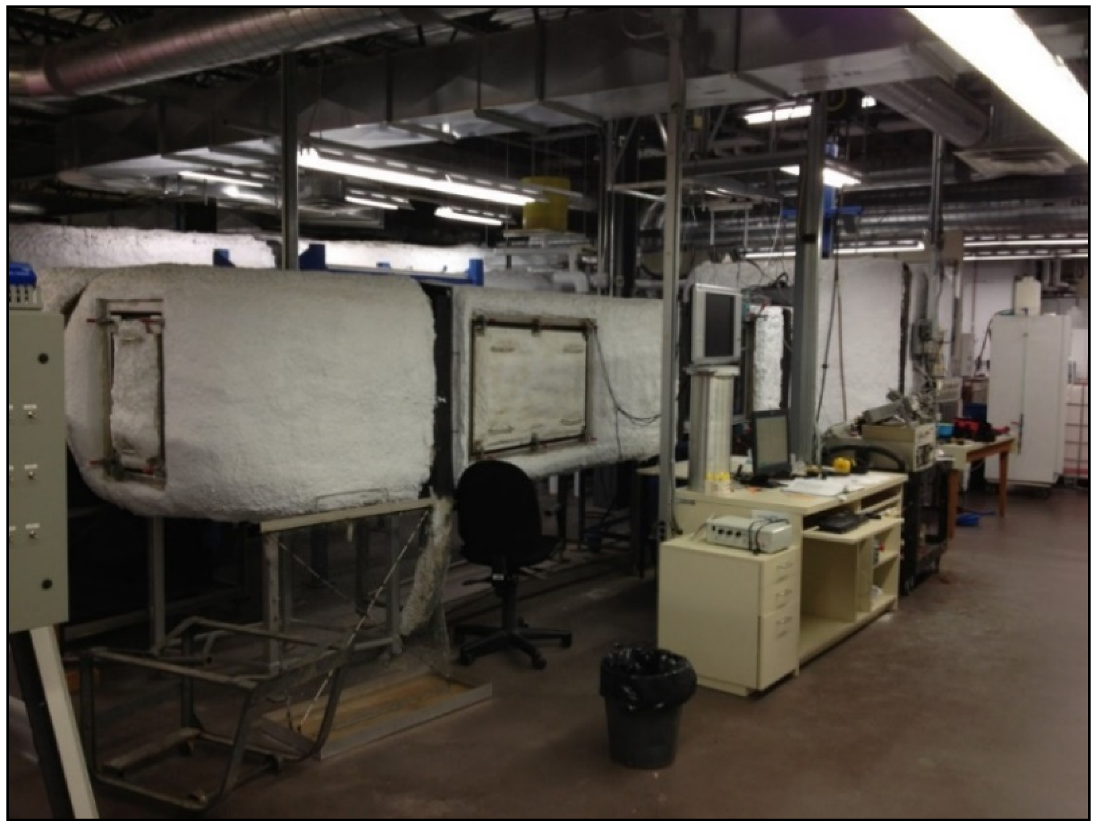
2.1. Icing Wind Tunnel (IWT)

Figure 1 shows a general photo of the IWT located at the AMIL in which all the experiments were conducted. The wind tunnel meets the conditions of the SAE Aerospace Recommended Practice for icing wind tunnel ARP5905 [50] and Aerospace Information Report for droplet sizing AIR4906 [51]. The IWT is a closed-loop low-speed refrigerated wind tunnel able to operate at sub-zero temperatures at sea level pressure and has two test sections. The test section used is 0.91 m in width by 0.76 m in height and tests can be run at air speeds of up to 50 m/s at room temperature. The IWT test section air speed (which is calculated by the Bernoulli equation) is controlled by computer via a control program and data acquisition card. The tunnel is a closed recirculating type that cools the flow immediately downstream of the test section. The refrigeration system capacity can vary the total air temperature between −48 and 22 °C. This is achieved by passing the air through a heat exchanger of 1.6 m by 1.6 m, powered by a compressor and a glycol pump.

A water spray system is used to generate the icing cloud. It consists of three spray ramps, having eight to nine air atomizing nozzles each, and composed of pneumatic sprinklers (Figure 2). The water line is under pressure and rotameters control the flow rate to meet the desired liquid water content while the water droplet diameter is controlled by the air pressure injected into the nozzle. A cooling unit controls the water temperature used to produce a cloud of supercooled water droplets with median volumetric diameters (MVD) ranging from 20 to 60 µm and liquid water content (LWC) ranging from 0.1 to 3.0 g/m³. The water is filtered and cleaned to obtain osmotic de-mineralized distilled water. The spray system is located upstream of the center of the test section in the straight section (9) before the convergent (8), and oscillates up and down to cover, when necessary, the entire test section height (1) (Figure 2). The super-cooled droplets impinge on the test model in the center of the test section. During a test, the water flows continually, the air pressure is open when the test begins and the simulated cloud is formed in the IWT test section.

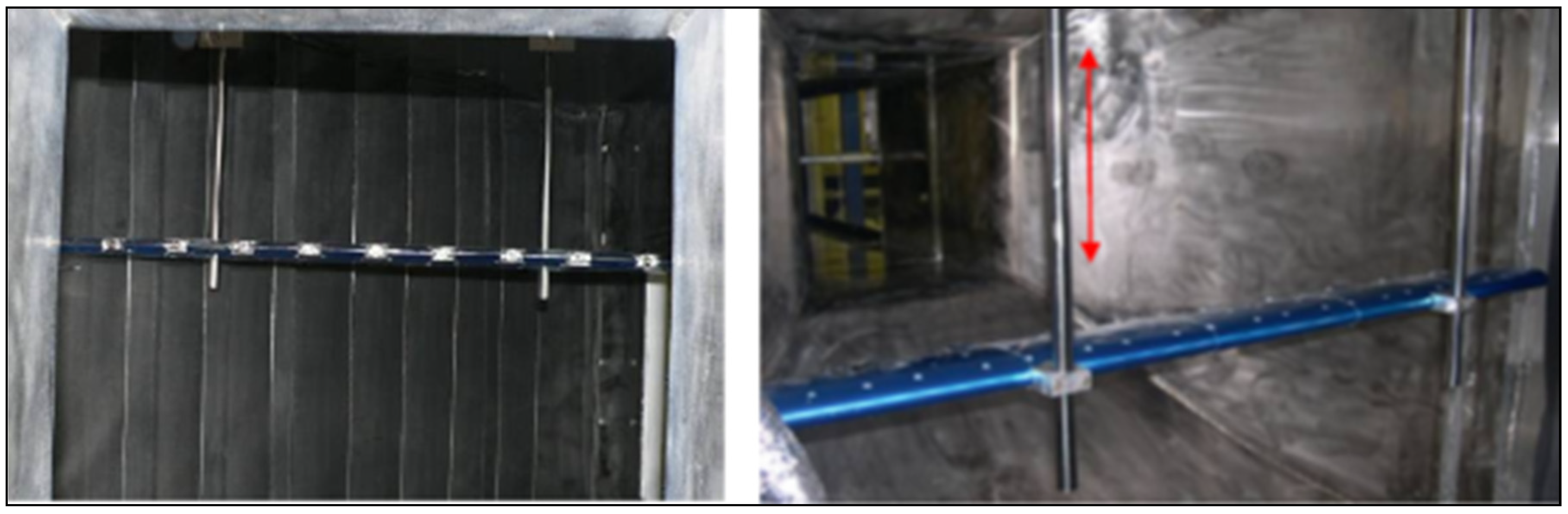
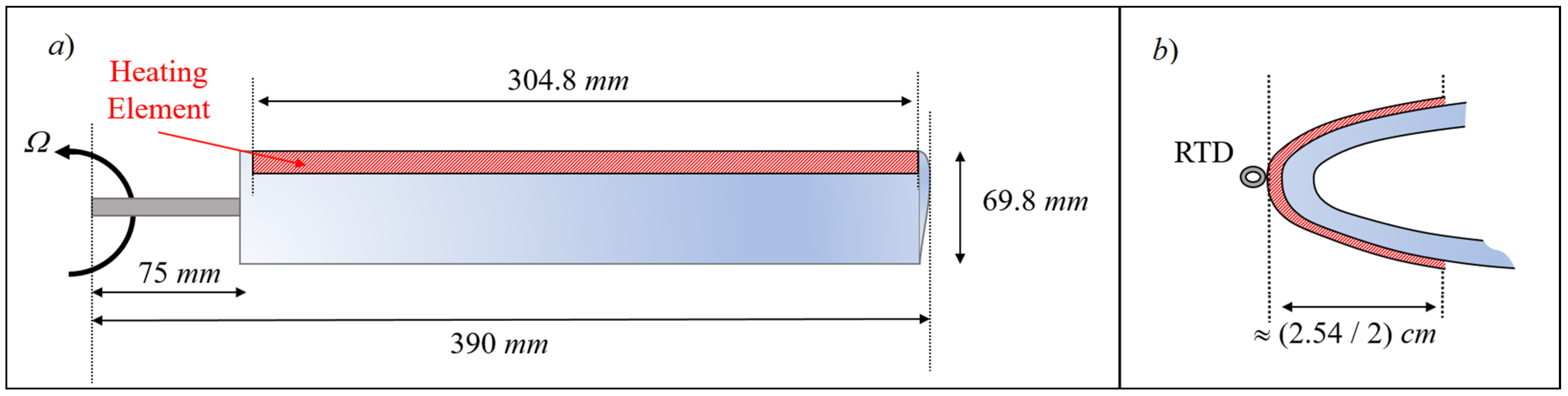
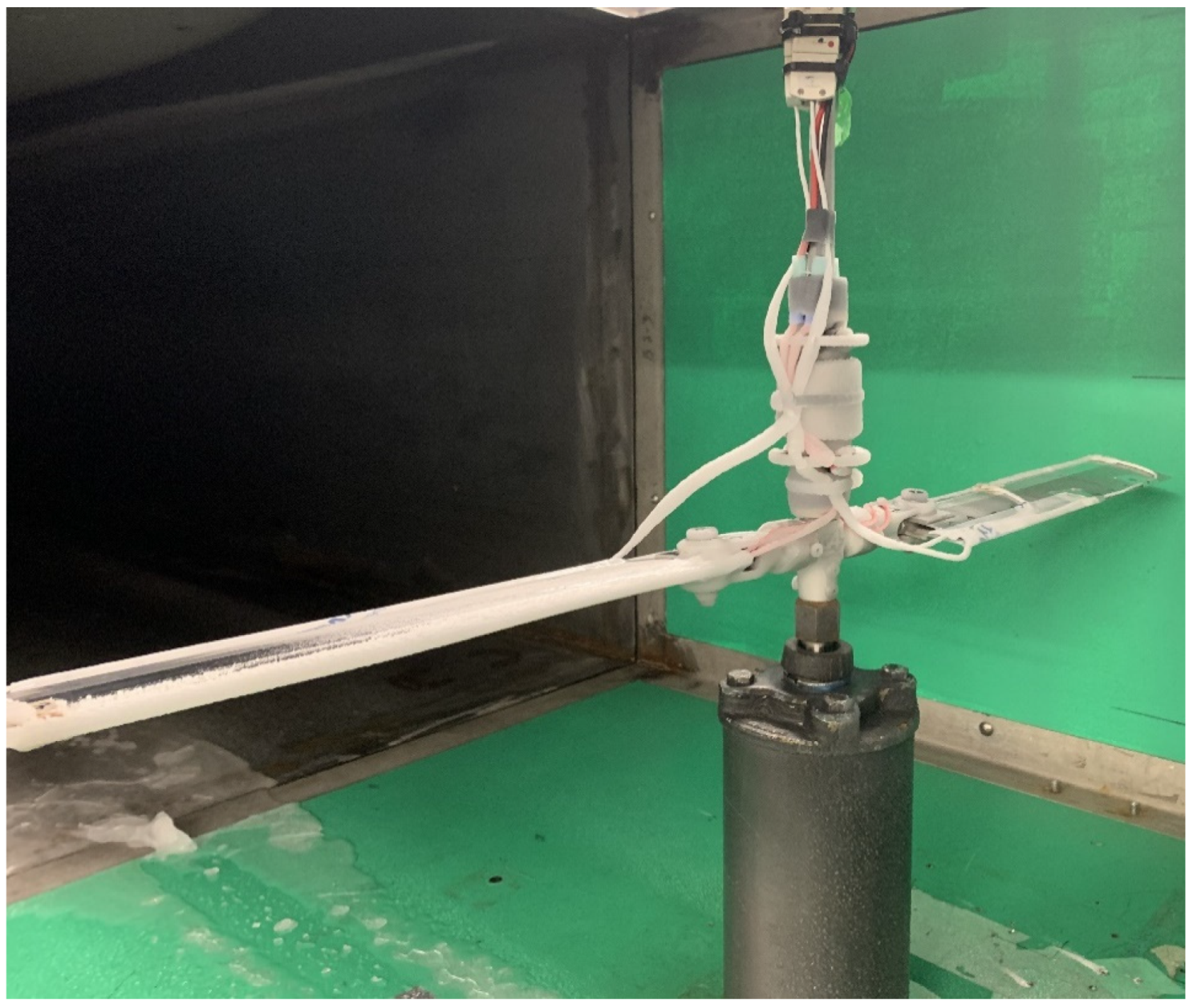
2.2. Powered Spinning Rotor Blade (P-SRB)

The Powered Spinning Rotor Blade (P-SRB) setup was designed by modifying the Spinning Rotor Blade (SRB) setup developed at the AMIL more than 10 years ago [26] and is the same setup used in [52]. The original setup is composed of two blades in horizontal rotation connected to a hub and driven by a motor and a power shaft transmission.

A IEC-FR-LC-10 Slipring by IEC Corporation (Austin, TX, USA) [53] is used to bring electrical power to the spinning blades of the P-SRB. The hub was connected to a 3600 RPM 10 hp motor by a 2.54 cm (1″) diameter power steel shaft connected to a 10 hp drive. For safety reasons, the maximum spinning speed was limited to 1000 RPM. Power to supply the heating elements was generated by an Elektro-Automatik (Viersen, Germany) EA-PS3150-04B laboratory power supply.

The rotor blades were untwisted extruded 6063-T6 aluminum with a mill finish used for tail rotor blades of small helicopters. The airfoil section had a NACA0012 profile and the blades characteristics are presented in

Table 1. P-RSB Geometric Characteristics.

Blade Root Distance	Blade Span (Radius)	Blade Chord
75.0 mm	390.0 mm	69.8 mm
Blade Twist	Blade Number	Material
0°	2	6063-T6 Al

and Figure 3a. The span is the rotor blade length from the rotation point to the blade tip. The length is the blade length from the hand attachment to the blade tip. More details on the P-SRB rotor setup have already been published and can be found in [52].

2.2.1. Heating Elements and RTDs

Figure 4 shows the complete setup of the experimented rotor. The leading edge of each blade was covered with a strip heating element that provided a constant heat flux once activated. The size of each heating element was 2.54 cm × 30.48 cm with a maximum power of 300 W as shown in Figure 3a,b. The elements are rectangular and do not change in shape across the length of the blade. The simple design of the elements was chosen to obtain the best grip possible on the rotor while testing. Although no study was performed on the effect of the heating element shape on the droplet impingement or collection efficiency, the experimental setup was carried out with the same heating elements in the tests with or without water spray, mainly to measure the temperature difference due to the addition of water spray.

The supplied voltage (U_V) and current (I_A) were varied according to each test. The total electric heating power was a direct result of the voltage and current variations. To help minimize losses, an aluminum tape was used to cover the heating element and to provide an even distribution of heat.

The Resistance Temperature Detectors (RTDs) were distributed across the radius of the blade to measure the temperatures at these different locations via a data logger at a rate of 5 recordings per second. The blade vibration rates were observed by the P-SRB software to guarantee stable rotation. For each test, a maximum of 3 RTDs could be fitted on the blade so at each test due to wiring limitations by the slip ring. The RTDs were placed at r/R = 0.6, 0.75 and 0.95. The non-dimensional radial location (r/R) was described by the ratio of the distance to the placed RTD by the tip radius of the blade. Due to experimental limitations, the RTDs were placed on the nose of the leading edge (S/c = 0), a point known to show some of the most elevated heat transfer rates [43,52]. More chordwise locations are scheduled for testing in the future.

2.2.2. Convective Heat Transfer

The air properties vary with temperature. Therefore, a reference temperature (T_f) was chosen to estimate those properties, similar to [43]. According to [54], the equation can be applied for a flow where V_∝ is a constant and the temperature does not vary markedly in the boundary layer. The density (ρ), viscosity (μ) and thermal conductivity of the air (k) were calculated at T_f through Equation (2). The Re employed in this analysis is based on the chord (Re_c) and calculated using Equation (3). (V_r) is the local velocity on each radial position of the blade calculated using Equation (4), with the two terms of velocity originating from the rotation of the blade and the air velocity in the wind tunnel. As Equation (4) indicates, the pitch angle will impact the calculated heat transfer. However, for the current study, the analysis is limited to one pitch angle.

$$T_f=\frac{T_{\infty }+T_{RTD}}{2}$$

(2)

$$R{e}_c=\frac{\rho V_{r}c}{\mu }$$

(3)

$$V_r=\Omega r+V_{\infty }\cos (\theta )$$

(4)

For the anti-icing tests, the heat transfer coefficient (h_RTD) was calculated using Equation (5) at each RTD. (Q_Elec) is the supplied electrical power. (Q_Rad) is the heat lost due to radiation, calculated using Equation (6). (Q_Cond) is the heat lost due to conduction in the blade aluminum material and is approximated at 4% to 8% of Q_Elec, based on previous work on the P-SRB [52]. (σ_SB) is the Stefan–Boltzmann constant and (υ) is the emissivity of polyimide (υ = 0.95). Finally, the local chord-based (Nu) was calculated using Equation (7), where (c) is the chord.

$$h_{RTD}=\frac{Q_{Elec}-Q_{Rad}-Q_{Cond}}{\left(T_{RTD}-T_T\right)}$$

(5)

$$Q_{Rad}={\sigma }_{SB}\upsilon \left(T_T^4-T_{RTD}^4\right)$$

(6)

$$Nu=\frac{h_{RTD}c}{k}$$

(7)

For the de-icing tests, each test was run until an approximate ice thickness of approximately 6 mm was accumulated on the furthest placed RTD (r/R = 0.95). The thickness of ice was chosen at the request of the industrial partner, with 6 mm being the maximum allowed to be accreted on the helicopter blades. Specifically, the thickness was measured using a digital caliper at the leading edge of the blade, where the RTD is located. Moreover, previous experiments at the AMIL showed that the accumulated ice on a rotor blade will vary in thickness from root to tip [26]. To estimate the ice thicknesses at r/R = 0.6 and 0.75, the ice was also measured for each test at r/R = 0.48 and an interpolation was performed between r/R = 0.48 and r/R = 0.95.

According to [42], heat transfer on the nose of the NACA 0012 leading edge may be approximated by the 1-D heat transfer equation of a cylinder in cross flow. Since this is the location where the measurements of this work are taken, the 1-D approximation to a cylinder is adopted to account for the conduction in the ice layer. Heat transfer in the ice is assumed to propagate perpendicularly between the air and the RTD below the ice layer. This way, Equation (5) is substituted by Equation (8), where an added term for the cylinder thermal resistance of the ice layer is incorporated [41]. (t_ice) is the ice thickness and (k_ice) is the thermal conductivity of ice. The Nu is then calculated using Equation (7). r₀ is the cylinder radius equivalent of a NACA 0012 leading edge, and is equal to 1.58% of its chord c [42].

$$h_{RTD}={\left[\frac{\left(T_{RTD}-T_T\right)}{Q_{Elec}-Q_{Rad}-Q_{Cond}}-\frac{\ln \left\{\raisebox{1ex}{$\left(r_0+t_{ice}\right)$}\!\left/ \!\raisebox{-1ex}{$r_0$}\right.\right\}}{2\pi k_{ice}}\right]}^{-1}$$

(8)

2.3. Rotor Testing Plan and Procedure

Table 2. Rotor Test Plan with Specific Test ID#.

Test Mode	V∝ (m/s)	500 RPM	900 RPM	1000 RPM	T∝ (K)	r/R	θ (°)
Anti-Icing	20	1	2	3	265.65	0.6, 0.75 and 0.95	6
	30	4	5	6
De-Icing	20	7	8	9	265.65
	30	10	11	12
De-Icing	20	13	14	15	258.15
	30	16	17	18

shows the details for all tests conducted on the rotor. All tests were performed at θ = 6° and the freestream velocity was either V_∝ = 20 m/s or V_∝ = 30 m/s. Three different rotor speeds were used (Ω = 500 RPM, 900 RPM and 1000 RPM) as well as two air temperatures (T_∝ ≈ 258.15 K and T_∝ ≈ 265.65 K). Tests were performed both in the anti-icing mode and in the de-icing modes, which are detailed later in the next sections. In total, 18 tests were performed each having a unique ID# for easy referencing.

2.3.1. Anti-Icing Tests

The anti-icing tests were performed with the following 3-step sequence: (1) spin the rotor with the heaters activated and no water spray, until the temperature at r/R = 0.95 stabilizes at the steady-state target temperature of T ≈ 280.15 K; (2) activate water spray and adjust heating power until the temperature at r/R = 0.95 stabilizes at approximately T ≈ 280.15 K; (3) lower heating power until the temperature at r/R = 0.95 stabilizes at approximately T ≈ 267.15 K or until ice accretion on the blade’s leading edge begins.

Figure 5 shows a close-up photo of the blade taken at the end of anti-icing test #5. The leading edge is ice free due to the continuous operation of the heaters underneath the aluminum insulating tape, but ice began to appear at the tip due to the gradual lowering in power applied. Ice was present behind the leading edge, mainly due to water runback that froze downstream of the chord where no heaters are present.

A sample of the results of the anti-icing tests conducted is shown in Figure 6 (test #1). Results are shown in terms of the Nu (calculated based on Section 2.2.2) variation versus the test time in seconds. The first step of the testing sequence extends from t = 0 sec until the first shown dashed black line. The latter represents the initiation of the water spray (step 2), while the second dashed black line marks step 3, when the power is lowered, and ice traces are formed.

Two regions of interest are identified in the subfigures of Figure 6. The first is identified as the “dry” region where no water was sprayed and is located before the first dashed black line. The second is identified as the “wet” region, when the water spray was initiated and is found between the two dashed black lines. For each of the tests, the average Nu for the dry case (Nu_Dry) was calculated as the mean of Nu(t) in the 45 s before the first dashed black line, when the Nu(t) had stabilized. Similarly, the average Nu for the wet case (Nu_Wet) was calculated as the mean of Nu(t) in the 45 s before the second dashed black line.

2.3.2. De-Icing Tests

For the de-icing tests, ice was present on the blades since the start of the tests, and the heating power was adjusted until the ice is shed. With the presence of an ice layer, it was decided to investigate the heat transfer rate at two different freestream temperatures, T_∝ ≈ 265.65 K and T_∝ ≈ 258.15 K that are related to different types of ice (glaze and mixed glaze/rime ice). The tests were performed with the following 2-step sequence: (1) Rotate the blades until an ice layer of approximately 6 mm is formed on the leading edge at r/R = 0.95. (2) Turn on heaters and slowly increase heating power until the ice is shed from the blade.

Figure 7 shows two photos taken during de-icing test #11. Figure 7a shows the accumulated ice across the blade radius on both the upper and lower surfaces. It seemed that the ice accretes further downstream of the chord on the bottom surface of the blade, mainly due to the imposed positive pitch. In Figure 7b, the ice is clearly shed after the heaters are turned on and the power is increased until a break-off is achieved. In this specific test, no runback ice accumulation was seen, however the blade tips still had some ice.

Figure 8 shows a sample of the results of the conducted de-icing tests (specifically, test #9). Results are shown in terms of the Nu variation versus the test time in seconds. The first step of the testing sequence is not shown in the figures, meaning the ice layer is already present at t = 0 sec and no heating occurs. The second step extends from t = 0 sec until the dashed black line. The latter represents the detachment of the ice layer from the blade. It should be noted that the ice layer detaches from blade #1, where no RTDs are placed, whereas on the blade #2 (where measurements are reported) the ice does not detach, most likely due to the RTDs holding it on the surface. In only one test did the ice layer detach from the tested blade.

Since the ice layer did not detach off the blade, the time at which the ice detached off the other blade was recorded. The Nu(t) before this instant was calculated based on the 1-D approximation of heat transfer with the 6 mm ice layer and is referred to as Nu_Ice. The main interest lies in the Nu_Ice while the Nu in the detached region (where an accelerated jump in Nu(t) values is seen) only signifies that ice had detached on the other blade and is not used in this paper.

2.4. Experimental Error Estimation

The method of [55], represented by Equation (9), is used to estimate the uncertainty in heat transfer measurements. It describes the error in the measurement of the electric heat input Q_Elec. The errors originating from the calculation of Q_Rad and Q_Cond is neglected since they were found to represent a fraction of the total Q_Elec (between 1% and 8%). Therefore, the error due to those two terms was very small (<0.5%).

$$\frac{\partial h}{h}=\sqrt{{\left[\frac{\partial \left(T_{RTD}-T_{\infty }\right)}{\left(T_{RTD}-T_{\infty }\right)}\right]}^2+{\left[\frac{\partial I_A}{I_A}\right]}^2+{\left[\frac{\partial U_V}{U_V}\right]}^2}$$

(9)

The three main sources of the error in Equation (9) are: (1) temperature measurements, (2) voltage fluctuations and (3) current fluctuations. The error from temperature measurements was determined to be approximately 1%. The voltage fluctuations represented an error of 2.6% and the current fluctuations represented an error of 3.9%. The total uncertainty is therefore 7.5%.

The randomness error of the tests was calculated by repeating de-icing tests #11 and #17 four times each. Similar test conditions were run along with similar icing times and thicknesses, the power was increased during tests until the ice is shed. The power at which ice shedding occurred was recorded for each repetition and the range of powers recorded is presented in

Table 3. Range of Powers and Error between Test Repetitions.

Test ID#	Power Range (W/m2)	Error
11	6045–6355	5%
17	11,780–14,570	19%

. The repetition error was calculated by being the percentage discrepancy between the highest and lowest power recorded. According to Table 3, the randomness error could be as high as 19%, and considering the uncertainty in heat transfer measurements, the total experimental error could then be rounded to 26%.

3. Results

The main goal of this section is to analyze the behavior of the Nu_Dry, the Nu_Wet and the Nu_Ice with Ω, V_∝ and r/R. For the de-icing tests, the effect of the T_∝ on the Nu_Ice is also investigated. In the foregoing analysis, the Nu_Dry values are taken as reference to compare the Nu_Wet and the Nu_Ice.

3.1. Anti-Icing Tests

In this section, the results of the tests performed in the anti-icing mode are investigated. The heating power was adjusted during the tests to prevent any ice formation. The Nu_Dry is calculated before the water spray is activated. The Nu_Wet is calculated after starting the water spray with LWC = 0.8 g/m³.

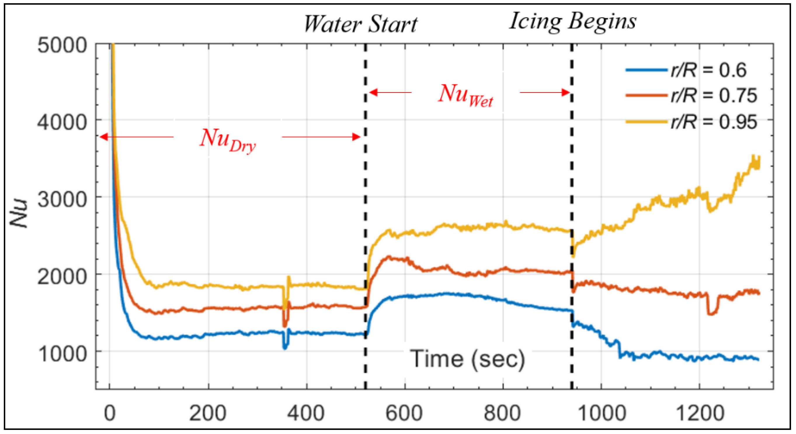
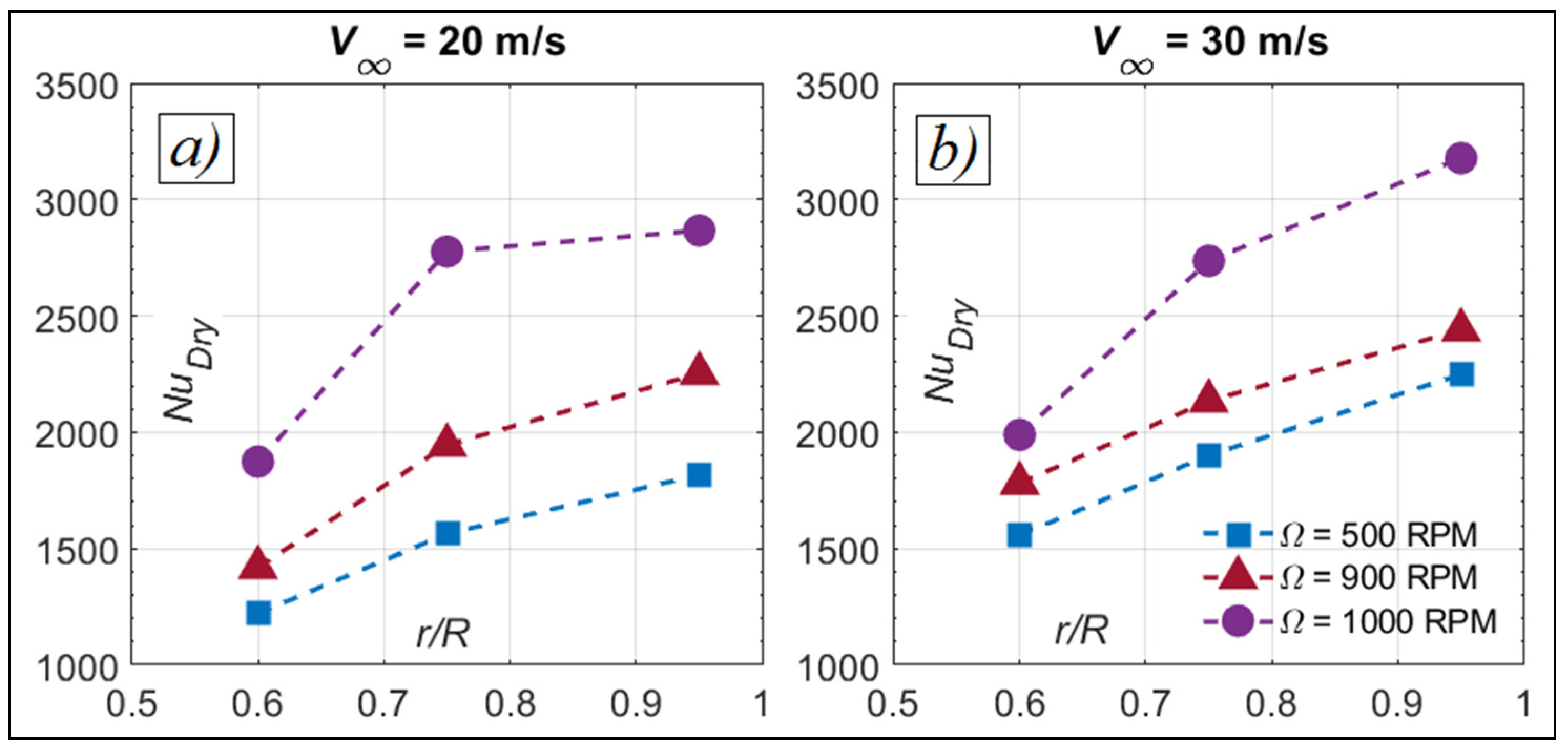
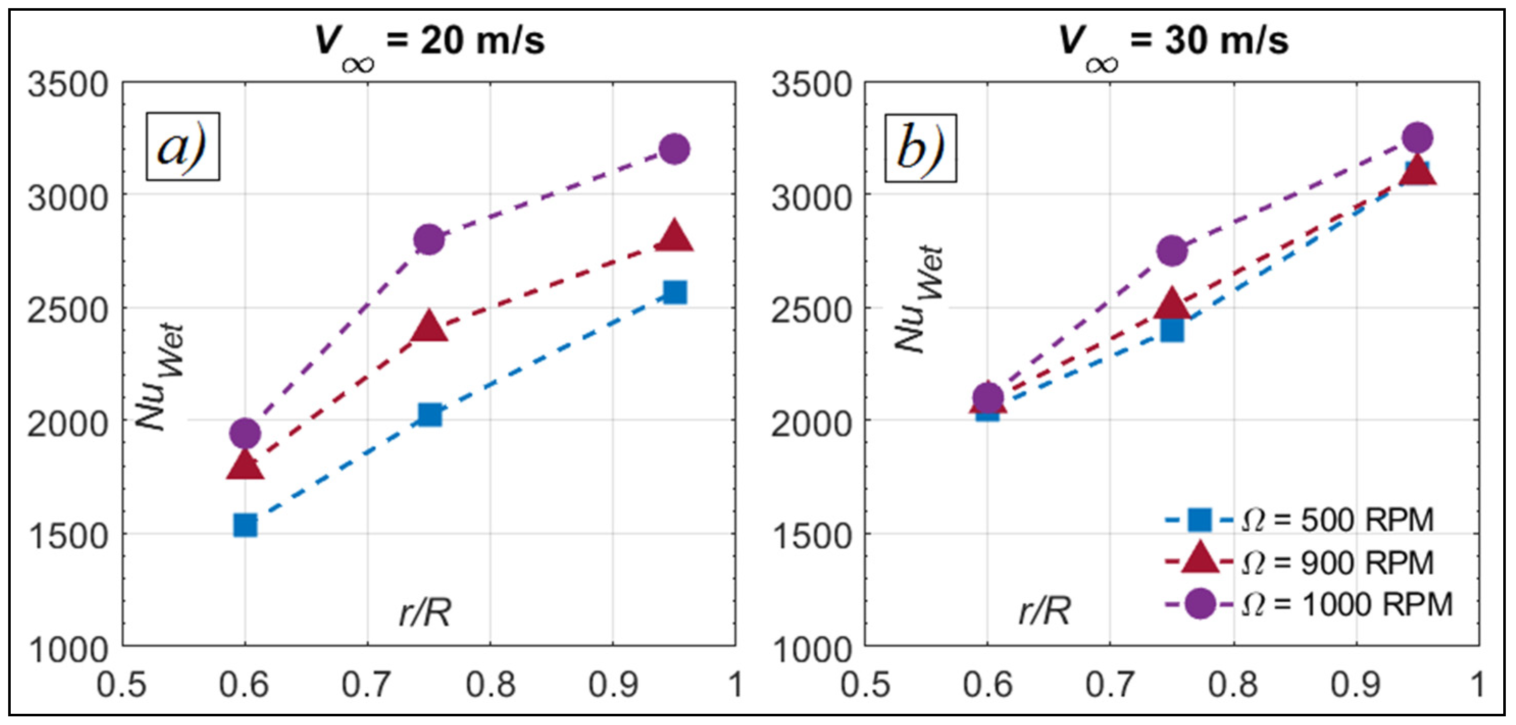
3.1.1. Nu_Dry and Nu_Wet Variation with r/R and Ω

Figure 9 shows the variation in the calculated average Nu_Dry for the tests performed at V_∝ = 20 m/s (Figure 9a) and V_∝ = 30 m/s (Figure 9b) with respect to r/R. In terms of the effect of r/R, the Nu_Dry increases as the point of measurement moves closer to the blade tip, regardless of the Ω or V_∝, mainly due to the increase in Re with rotation. The Ω had a similar effect on the Re and therefore, the Nu_Dry increases with an increasing Ω. Finally, the increase in V_∝ also showed an increase in the Nu_Dry, where the Nu at the same r/R is higher for the tests at V_∝ = 30 m/s compared to those at V_∝ = 20 m/s. In a similar analysis, Figure 10 shows the variation in the calculated average Nu_Wet for the tests performed at V_∝ = 20 m/s (Figure 10a) and at V_∝ = 30 m/s (Figure 10b) with respect to r/R. A similar trend to what was seen for the Nu_Dry can be observed. Generally, an increase in r/R, Ω or V_∝ caused a direct increase in the Nu_Wet.

3.1.2. Nu_Dry and Nu_Wet Variation with V_∝

Figure 11 shows the results of comparing the effect of V_∝ on the calculated average Nu_Dry and Nu_Wet for each of the tests. Figure 11a shows the ratio of the Nu_Dry obtained at the tests at V_∝ = 30 m/s to the tests at V_∝ = 20 m/s, whereas Figure 11b shows the ratio of the Nu_Wet obtained at the tests at V_∝ = 30 m/s to the test at V_∝ = 20 m/s.

Starting with the comparison of the Nu_Dry at different V_∝, Figure 11 shows that the increase in V_∝ directly increased the Nu due to an increase in the Re. The Nu_Dry ratio at r/R = 0.6 was higher (between 1.07 and 1.29) compared to that at the other r/R (between 0.98 and 1.24). The smaller radius contributes to a smaller velocity component due to rotation, and an increase in V_∝ at r/R = 0.6 shows a larger influence on the Nu than the other r/R.

The Nu_Wet ratio also increased because of an increasing V_∝. This changed in parallel with a drop of the Nu_Wet ratio as the Ω was increased. Similar to the Nu_Dry ratio, the Nu_Wet ratio was highest at the smallest r/R, mainly due to the increase in Re across the blade. For the three tested Ω, the Nu_Wet ratio was between 1.09 and 1.33 at r/R = 0.6 and between 0.98 and 1.2 at the other r/R.

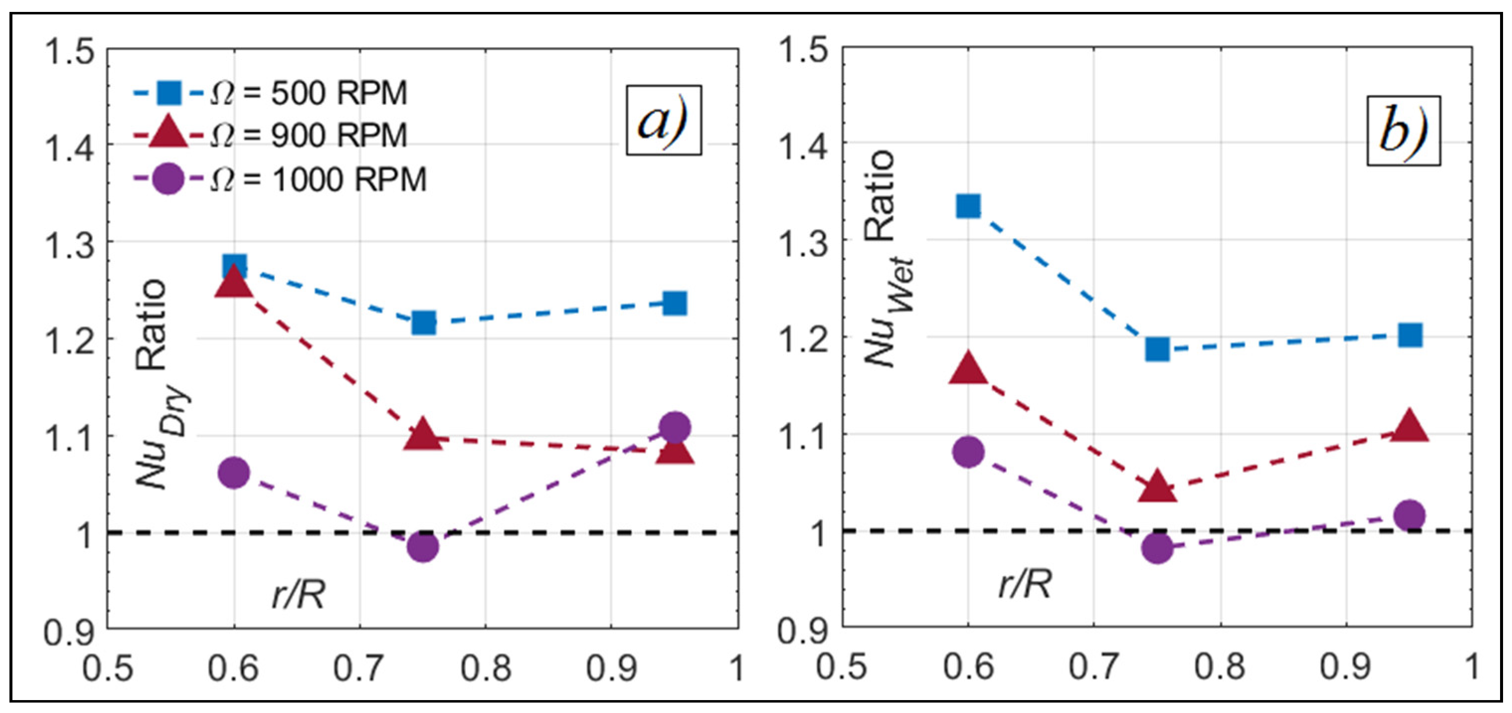
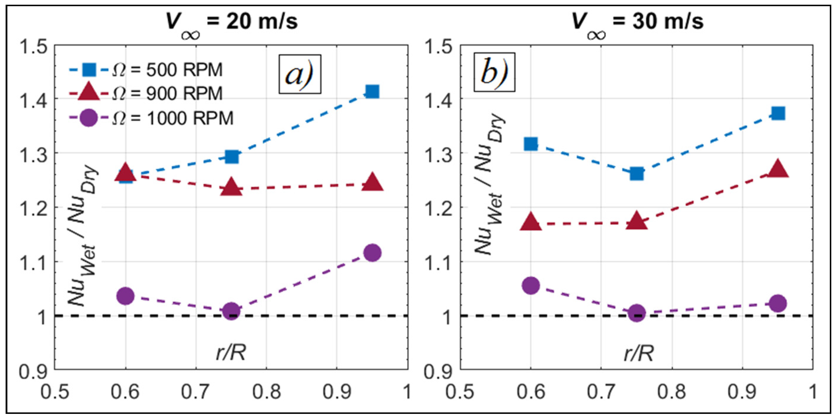
3.1.3. The Nu_Wet to Nu_Dry Ratio

Figure 12 shows the results of comparison between the wet and dry values of the calculated average Nu for each of the tests. Figure 12a shows the Nu_Wet to Nu_Dry ratio for the tests at V_∝ = 20 m/s. Similarly, Figure 12b shows the Nu_Wet to Nu_Dry ratio for the tests at V_∝ = 30 m/s. The Nu_Wet to Nu_Dry ratio was always larger than 1, which is expected due to the added water spray. The ratio was also similar between the tests with the different V_∝, with no significant difference between the two. The findings of Figure 12 are consistent with those of [48]. Using similar LWC and Re to the present work, Wang et al. reported that the addition of the water spray (on a fixed wing NACA 63-421 airfoil) increases the Nu_Avg values by an average of 26%.

Moreover, the Nu_Wet to Nu_Dry ratio decreased with an increasing Ω and the largest ratio was mostly seen at r/R = 0.95, varying between 1.41 and 1.05 depending on the Ω. This could be explained by the concentration of the water collection amount that is maximum near the tip of the blade, as seen in [38]. In their numerical simulation of a rotor in forward flight, they showed that the water collection amount increases from root to tip and is maximum around the stagnation region.

3.2. De-Icing Tests

In this section, the results of the tests performed in the de-icing mode are analyzed. Ice was present on the blades since the start of the tests, and the heating power was adjusted to achieve ice break-off. With the presence of an ice layer, it was decided to investigate the heat transfer rate at two different freestream temperatures, T_∝ ≈ 265.65 K and T_∝ ≈ 258.15 K.

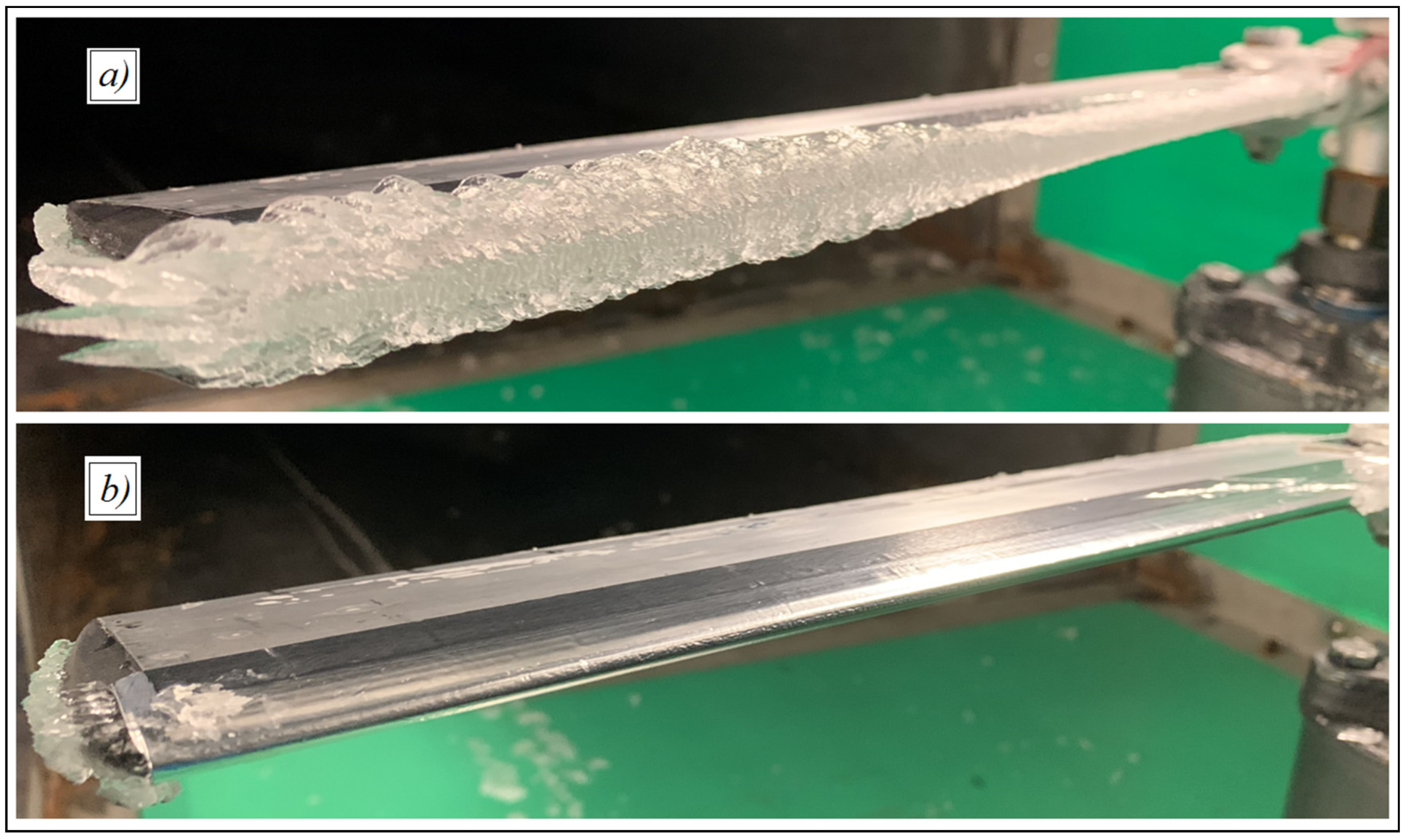
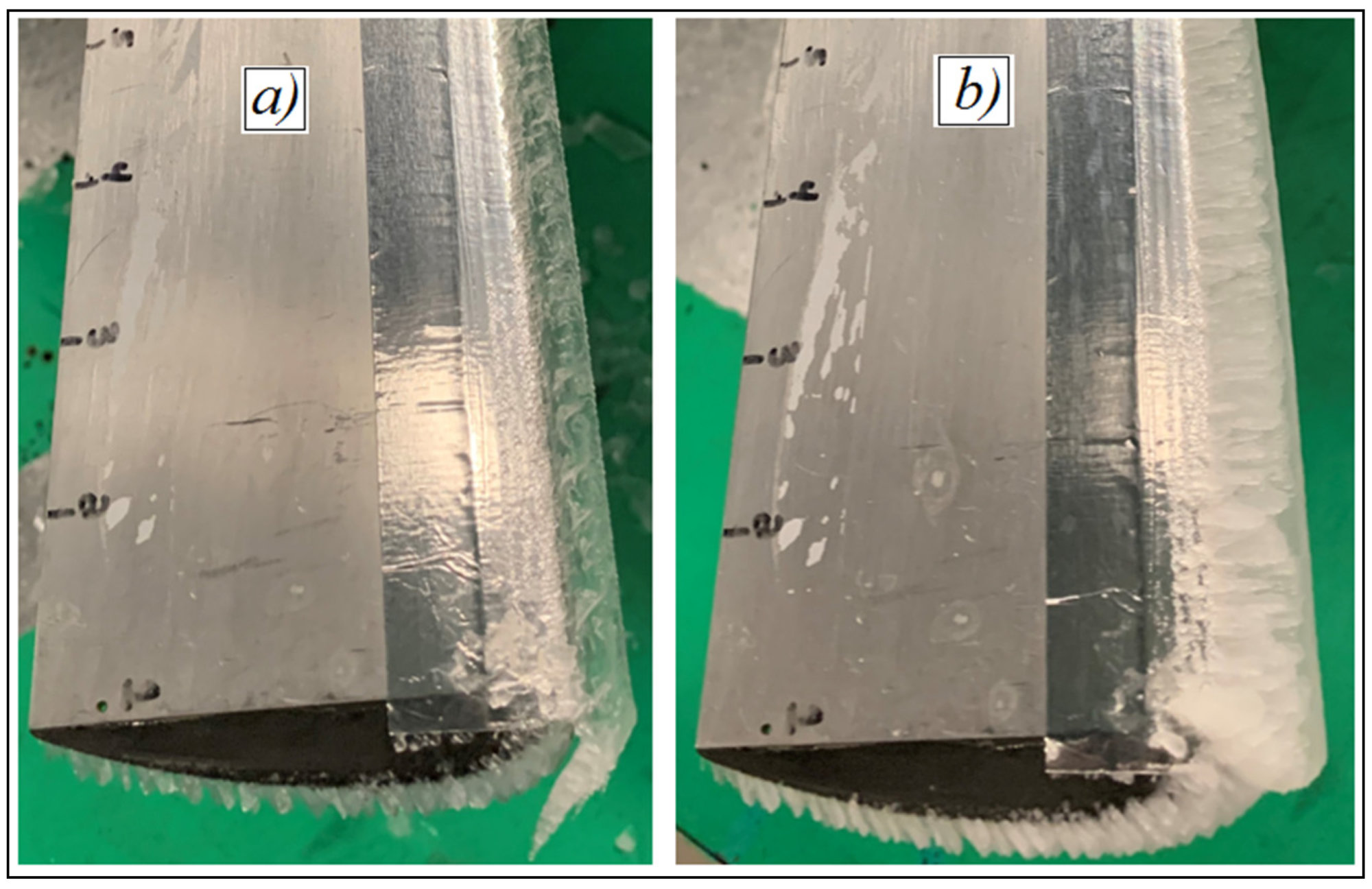
3.2.1. Measured Ice Thicknesses

Table 4. Measured Ice Thicknesses t_ice (in mm) of De-Icing Tests at r/R = 0.48 and r/R = 0.95.

r/R—Test ID#	7	8	9	10	11	12
0.95	6.04	6.32	7.99	6.18	6.03	6.14
0.48	5.56	5.51	6.83	4.93	5.46 *	5.50
r/R—Test ID#	13	14	15	16	17	18
0.95	6.29	6.64	10.02	5.56	5.79	5.63
0.48	5.47	4.47	6.38	4.26	5.73	5.45

presents the measured t_ice at two different radial locations of the blade for the de-icing tests after ice accretion. These values were used in the calculation of the h_RTD and the Nu_Ice in Equation (8). Although that actual thicknesses at r/R = 0.6 and r/R = 0.75 were not measured, they were interpolated based on the values in Table 4. The measurement at r/R = 0.48 for test #11 (indicated by * in Table 4) due to a methodological error but was later estimated based on visual inspection of the test photographs.

Results indicate that t_ice increased heading towards the tip, indicating that the blade rotation had a strong influence on the resulting ice shape. Most of the tests resulted with an ice thickness of approximately 6 mm (±0.5 mm) at r/R = 0.95.

For tests #9 and #15, up to 10.02 mm were accreted. Later investigations showed this was the result of a grain in the spray nozzle. The controlled icing conditions slightly changed and ice therefore accreted faster than expected. The Nu_Ice of these tests is later examined to determine if the different t_ice affect the correlation attempt.

3.2.2. Effect of T_∝ on Ice Type

The de-icing tests at different T_∝ produced different types of ice that can be visually identified in Figure 13. In Figure 13a, the ice shape near the blade tip obtained by test #8 (T_∝ = 265.65 K) is clear and almost transparent—properties of glaze ice. The right side of the figure shows ice accumulation on the blade, obtained by the de-icing test #14 (T_∝ = 258.15 K). In this case, the ice is white and opaquer although some degree of transparency still exists. Therefore, a mixed glaze/rime ice characterizes the ice type in Figure 13b.

The ice shapes obtained in this work resemble what is obtained by the experiments of [25]. In the latter, rotor experiments from with comparable dimensions, LWC, V_∝ and Ω as well as the same T_∝ as the present experiments produced similar ice types and shapes as the ones in Figure 13. Specifically, they observed a glaze ice accretion at T_∝ = 268.15 K, rime ice at T_∝ = 258.15 K and a mixed glaze/rime at T_∝ = 263.15 K.

The results of this work showed that the Ω had an effect on the ice type as well. The tests at 500 RPM and T_∝ = 268.15 K showed only rime ice accumulation, mainly due to the weaker water collection on the blade associated with the low Ω. At the same T_∝ and for higher Ω, the water collection was also higher. The ice type was then similar to that seen in Figure 13b, which is a mixed ice type. In this work and to simplify the correlation attempt of the Nu_Ice, the ice type at T_∝ = 265.65 K is treated as glaze ice, whereas a mixed glaze/rime ice type is assumed for all tests at T_∝ = 258.15 K.

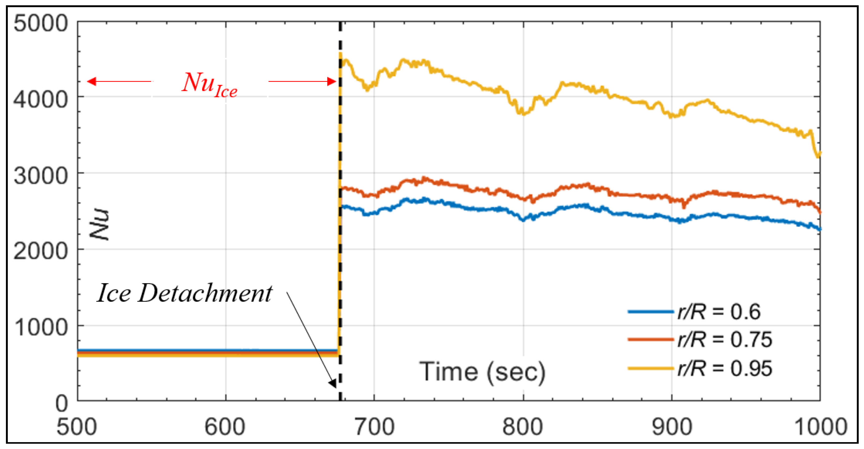
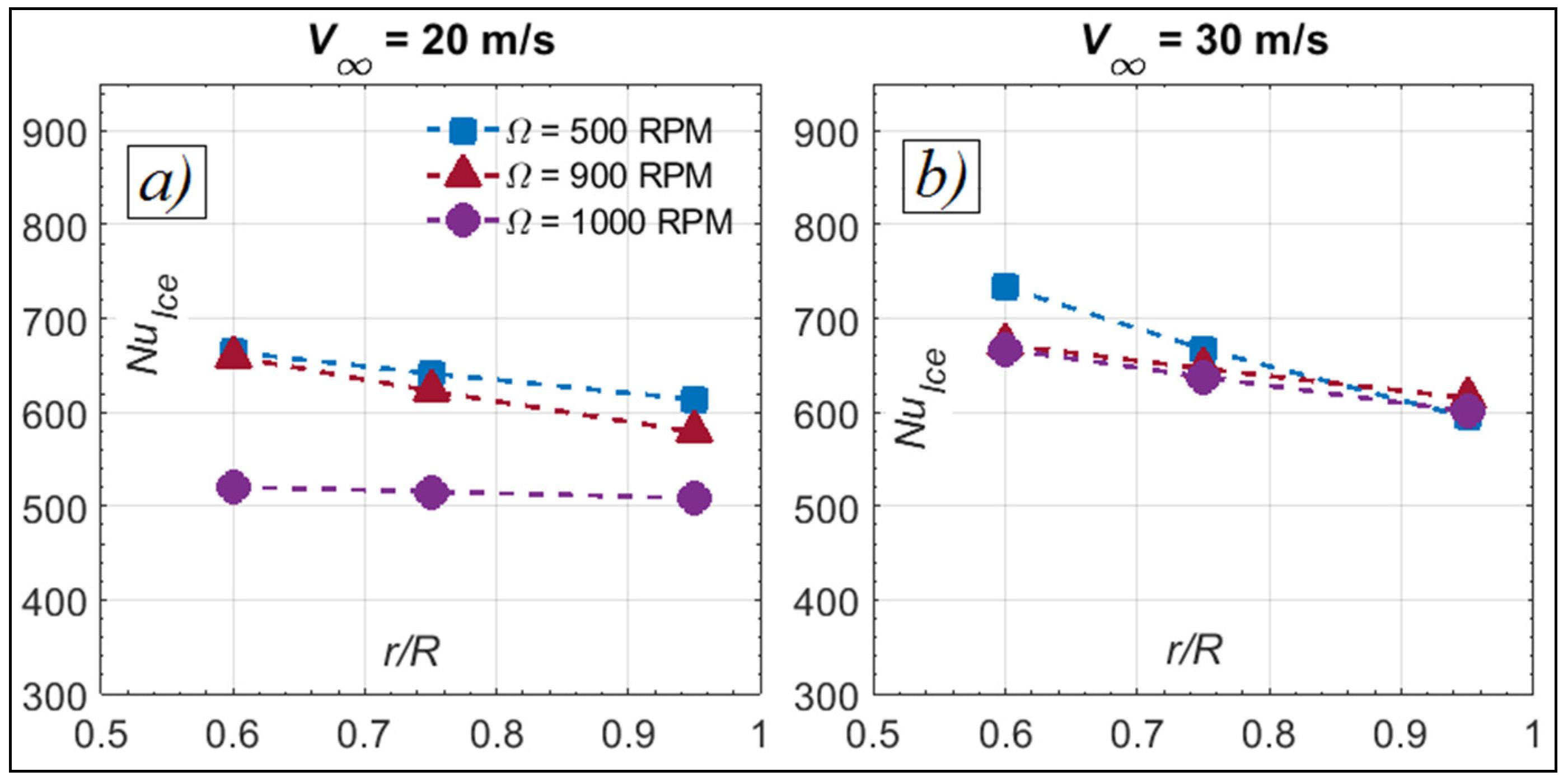
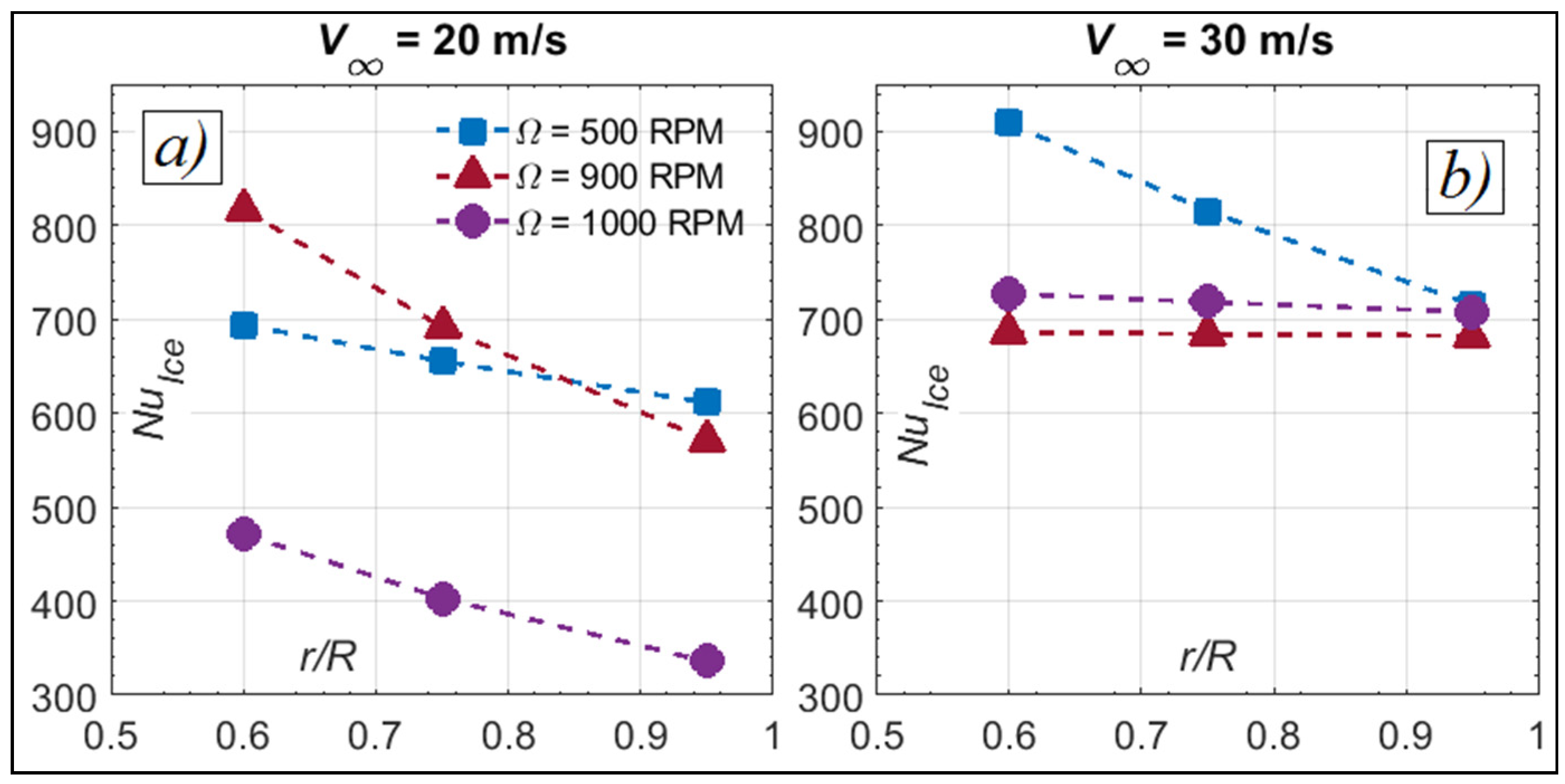
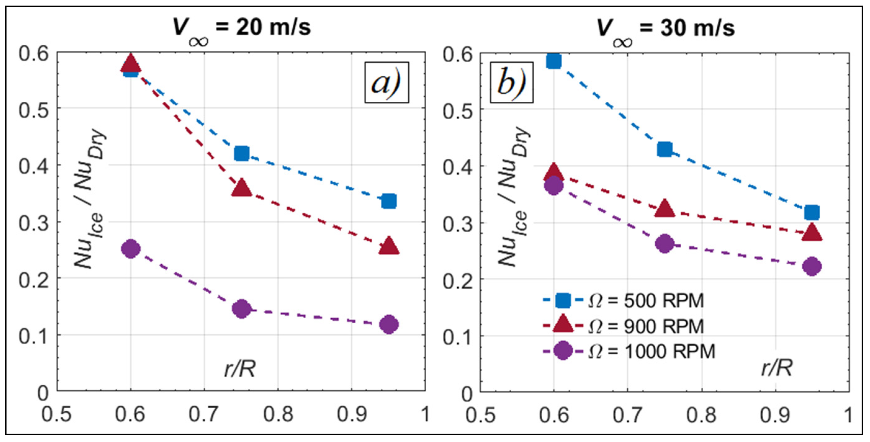
3.2.3. Results of Nu_Ice Variation

Figure 14 shows the variation in the calculated average Nu_Ice with respect to r/R for the tests performed at T_∝ = 265.65 K and for V_∝ = 20 m/s (Figure 14a) and at V_∝ = 30 m/s (Figure 14b). At first glance, the Nu_Ice decreased with r/R and Ω but increased with V_∝. However, it is thought that the ice thickness had the major effect on the Nu_Ice.

In fact, t_ice had a dominant effect on the variation in the Nu_Ice and this was determined based on two observations. First, the decrease in the Nu_Ice with r/R changes in parallel with the increasing ice thickness from root to tip. This was true for all tests shown in Figure 14 and as seen in Table 4. Second, test #9 (Ω = 1000 rpm; V_∝ = 20 m/s) showed significantly lower Nu_Ice values compared to the other tests. For that test, the thickness was approximately 8 mm near the tip of the blade, almost 2 mm larger than the other tests. Moreover, the dependency of the Nu_Ice on the ice thickness can also be seen for the tests at T_∝ = 258.15 K.

Figure 15 shows the Nu_Ice versus r/R for the tests at T_∝ = 265.65 K and for both tested V_∝. As noted in the previous section, the Nu_Ice was strongly linked to the ice thickness on the blade. For all tests, the Nu_Ice decreased between 0.6 ≤ r/R ≤ 0.95 where t_ice was increasing. Additionally, test #15 (Ω = 1000 rpm; V_∝ = 20 m/s) showed the Nu_Ice values much lower than the tests at other Ω which could only be explained by the larger ice thickness of approximately 10 mm.

From another point of view, tests #17 (Ω = 900 rpm; V_∝ = 30 m/s) and #18 (Ω = 1000 rpm; V_∝ = 30 m/s) showed that the Nu_Ice was almost constant between 0.6 ≤ r/R ≤ 0.95. Further examination of Table 4 indicates that for those tests, the difference of t_ice between 0.48 ≤ r/R ≤ 0.95 was very small. This led to nearly constant Nu_Ice, as seen in Figure 15 although the temperature gradient between the RTD and air was different between the tests.

Concluding, the examination of Nu_Ice variation indicate that it is strongly influenced by the ice thickness on the blade. However, when a comparable ice thickness is found between the different tests, the Nu_Ice is believed to decrease with Ω but increase with V_∞.

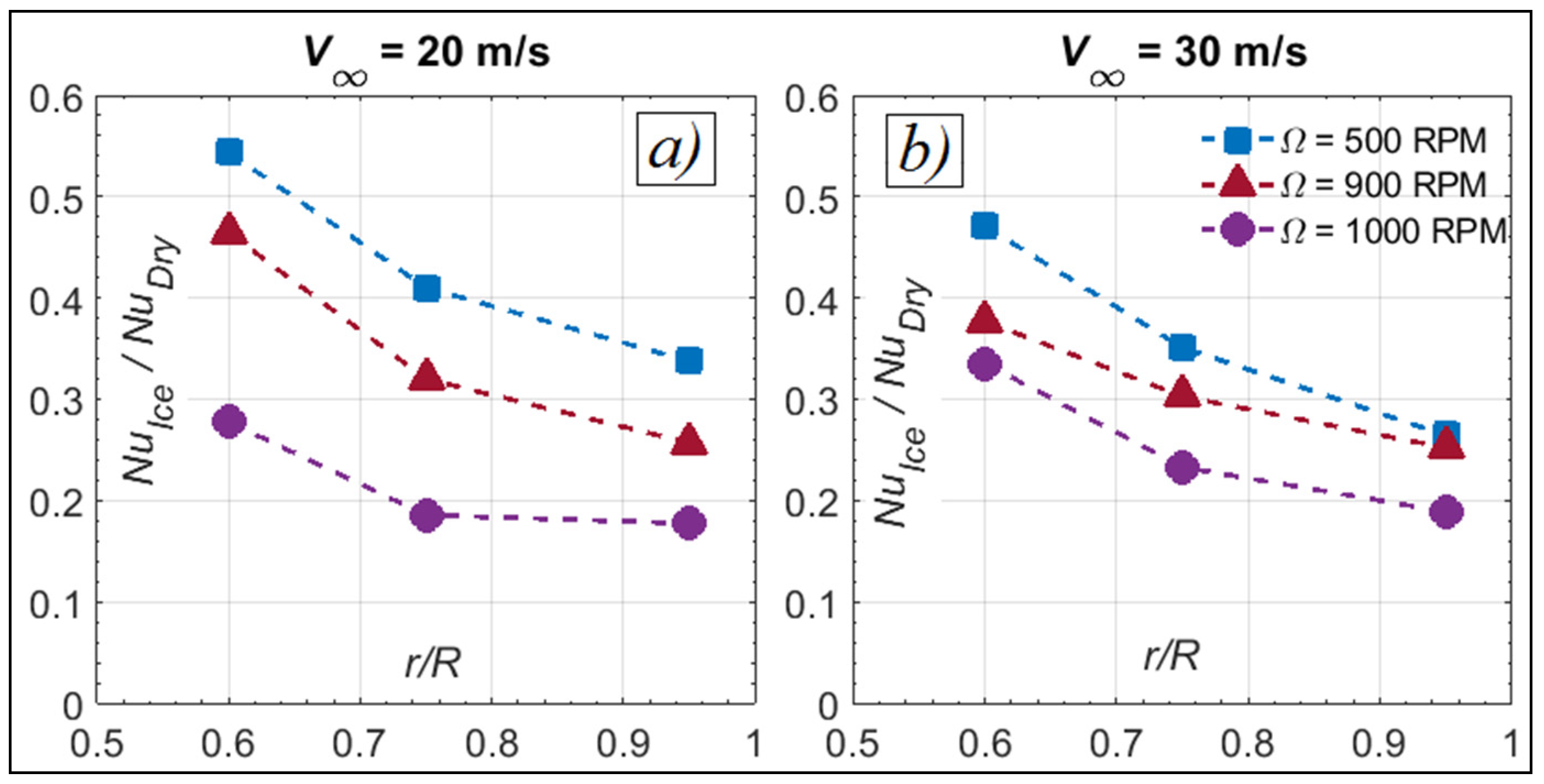
3.2.4. The Nu_Ice to Nu_Dry Ratio

The calculated Nu_Ice was also compared to the Nu_Dry obtained from the anti-icing tests. Figure 16 shows the variation in the Nu_Ice to Nu_Dry ratio of the tests at T_∝ = 265.65 K, while Figure 17 shows the same ratio but for the tests at T_∝ = 258.15 K. All test points indicate that the Nu_Ice is smaller than the Nu_Dry, with the ratio being always less than 1. The ice layer acts as an added insulation, reducing the theat transfer rates to the blade surface. Moreover, the ratio decreased when V_∝, r/R or Ω were increased.

Going towards the tip of the blade, the ratio decreased due to the generally thicker ice layer. The decreasing behavior was seen for all tests, regardless of the measured thickness of ice. Tthe increase in either Ω or V_∝ is seen therefore to enhance the convection from air and make it more dominant in the calculation of the heat transfer coefficient, thus justifying the drop of the Nu_Ice to Nu_Dry ratio with Ω and V_∝.

4. Discussion

The goal of the present experiments is to correlate the experimental data into a form that could be used for a rotor heat transfer numerical tool, so the gathered data were correlated in a similar fashion to what previous studies have attempted [40,43,46]. In those works, the Nu was correlated with the Re as shown in Equation (1), where the parameters A and m are determined via curve fitting of measured data.

In this study, the Re_Avg is used to build the correlations and is defined as the mean of the Re calculated at each r/R. The reason is that the Re at any blade section will vary throughout the test with any of Ω, V_∝ and r/R. As an example, Figure 18 shows the variation in calculated Re at the three r/R of anti-icing test #2 versus time. The triple dependency creates relatively large variations in the Re as shown in Figure 18, where the Re increases when the blade is in the advancing side and decreases in the retreating side of the blade. Therefore, the mean of the varying Re shown in Figure 18 was calculated first and later used in the correlation development.

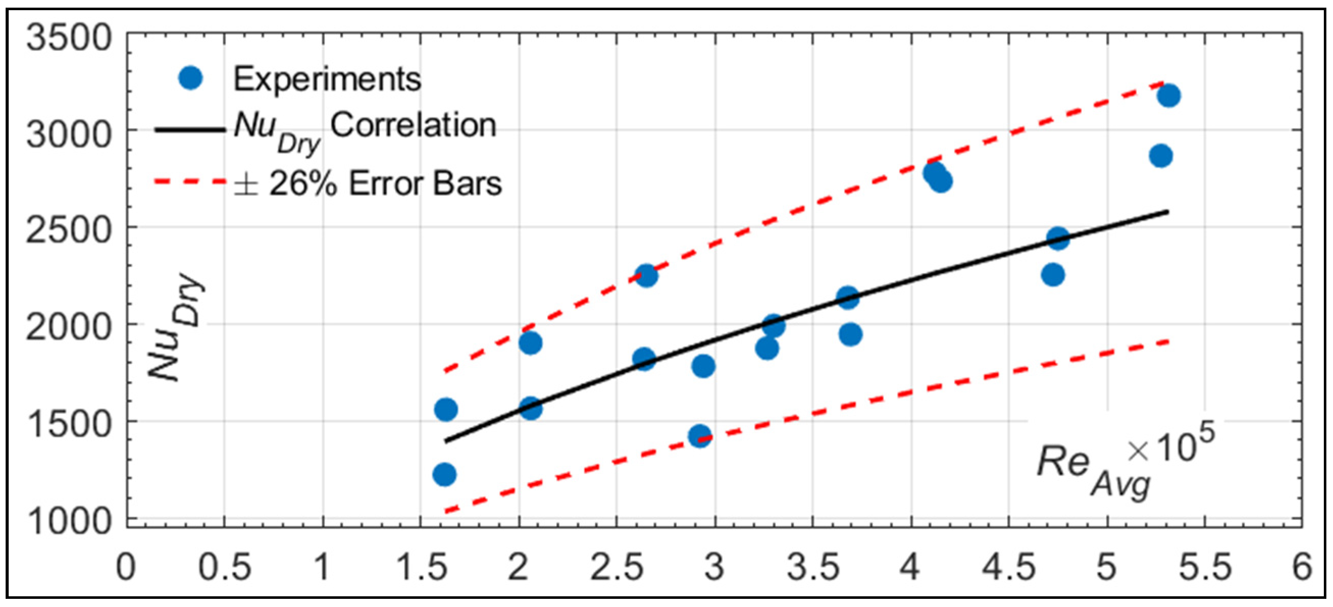
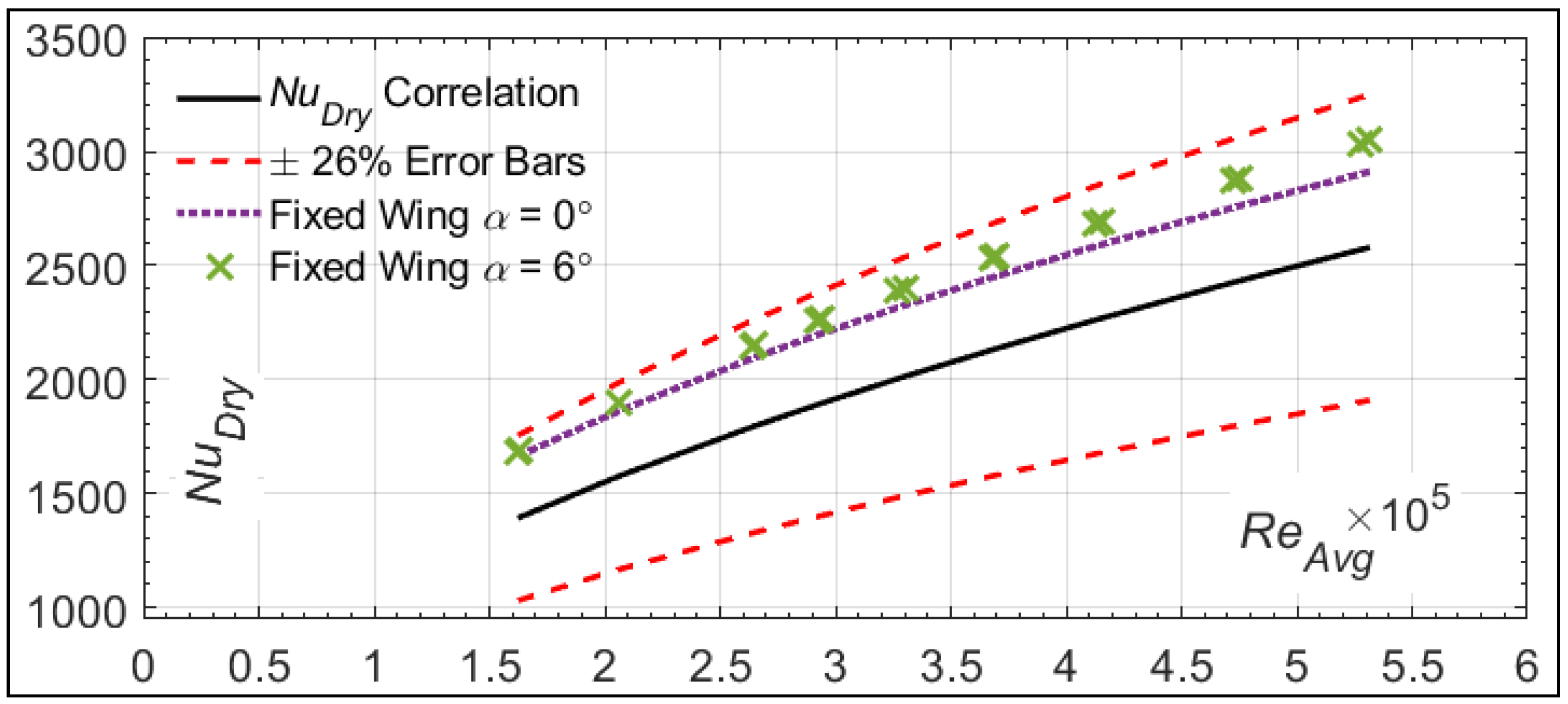
4.1. Correlation for the Nu_Dry

Figure 19 shows the variation in the Nu_Dry gathered by the experiments versus the Re_Avg of each test and r/R. In this paper, these values were fitted using a curve-fitting method by MATLAB based on the form of Equation (1) and the solid black line represents the best fitting of values obtained by the correlation. Moreover, the dashed lines show the ±26% experimental error accounted for by the correlation.

For the Nu_Dry, the correlation turned out to be in the form of Equation (10). For this fitting, the parameter m was determined to be m = 0.52, which is similar to what is expected for the flat plate in laminar flow [42] or for the stagnation and laminar region of an airfoil (near the leading edge) [43]. What this means is that for an analysis based on the Frossling Number Fr (which is the Nu divided by Re^0.5), the Fr would be independent of the Re_Avg. This again agrees with the findings of [42,43,56]. The average error between the prediction of the correlation and the experimental measurements was calculated at approximately 10%. The variation in the Nu_Dry recorded through the experiments therefore resembles what is expected from a laminar flow, and the correlation error could be explained by the total experimental error.

$$N{u}_{Dry}=3.04\times R{e}^{0.52}\times {\mathrm{Pr}}^{1/3}$$

(10)

For the sake of verification, Figure 20 compares the proposed correlation of this work to the correlations provided in the work of [43]. The correlations of the literature represent Nu values for a fixed wing with a NACA 0012 profile. Two α are included in the comparison and they are α = 0° and α = 6°. If the correlations from the literature are examined, Figure 20 shows that little effect was brought by changing the α. Although the point at S/c = 0 represented the stagnation point (maximum Nu) at α = 0°, only a slight drop of Nu values was seen at the same S/c when the α was increased. As explained in [43], this was due to laminar flow near the leading edge where the maximum occurred at S/c = 0 and a continuous decrease was noted further downstream.

When the correlation of Equation (10) is compared, a good agreement is seen with the correlations of [43]. The proposed Nu_Dry correlation agrees with the fixed wing data with a discrepancy of ≈ 15.9%. This is likely due to the experimental error encountered in the rotor tests, but this leads to the conclusion that the Nu_Dry near the leading edge of the rotor tests was well captured.

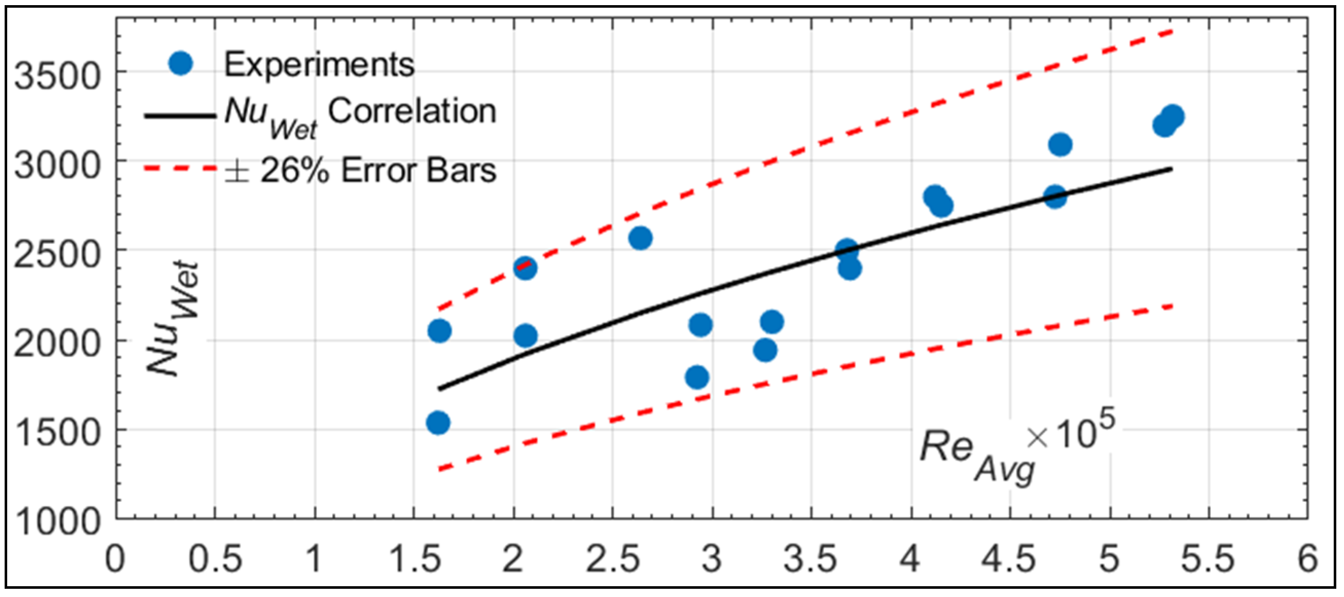
4.2. Correlation for the Nu_Wet

In a similar attempt to what was performed for the Nu_Dry, Figure 21 shows the variation in the Nu_Wet gathered by the experiments versus the Re_Avg of each test. The Nu_Wet was correlated based on the form of Equation (1) and the result is presented by Equation (11) where the average error was approximately 11%. The correlation is presented in the figure with the solid black line together with the ±26% error bars.

$$N{u}_{Wet}=8.16\times R{e}^{0.46}\times {\mathrm{Pr}}^{1/3}$$

(11)

All of the measured points lie between the ±26% error bars of the correlation. The datapoints that deviate the most from the correlation could be due to an ice accumulation near the tip of the blade, which is in turn a result of the small, unheated, zone at the ends of the heating element. The ice accumulation could have disturbed the flow and heat transfer, impacting the results. Without the ice formation and by accounting for the experimental error, the results of the Nu_Wet agree with the correlation (11).

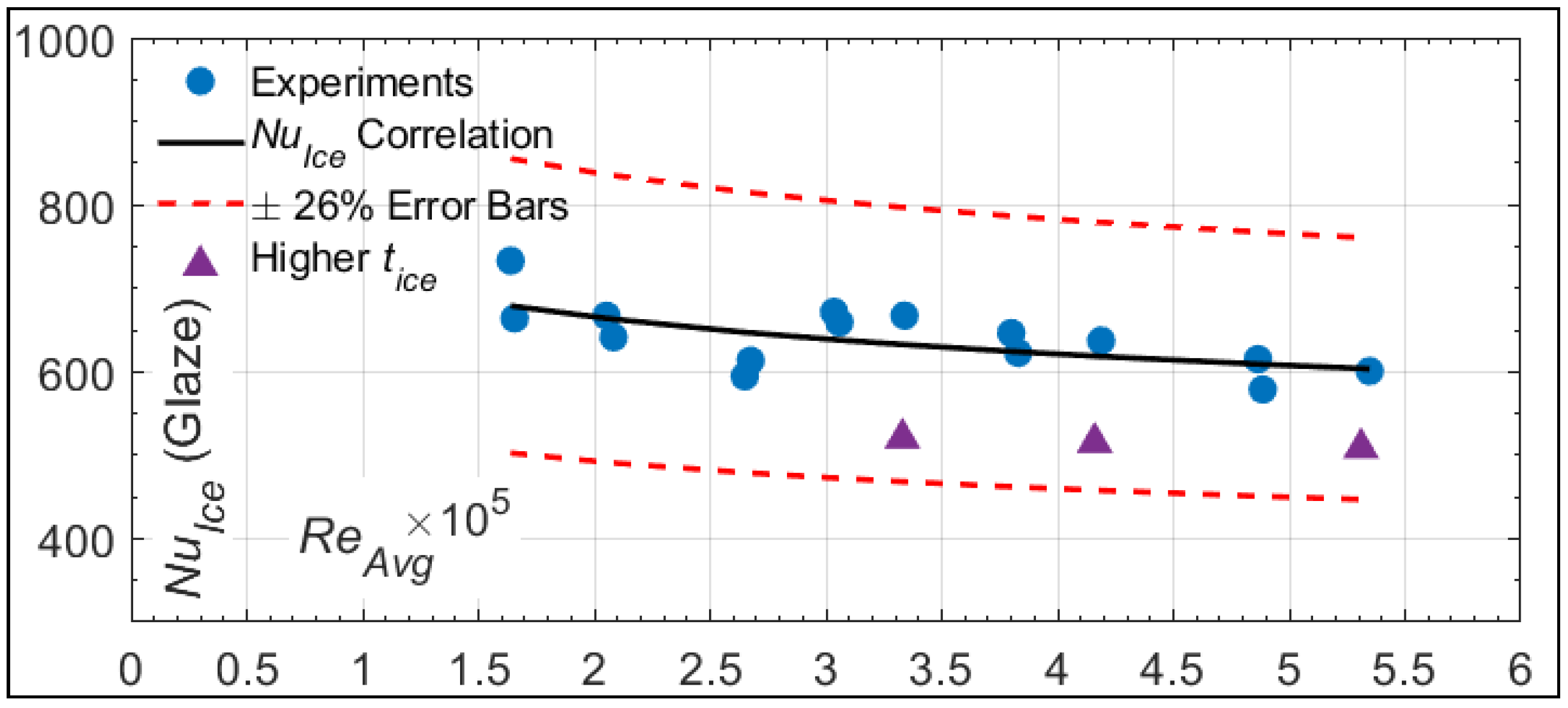
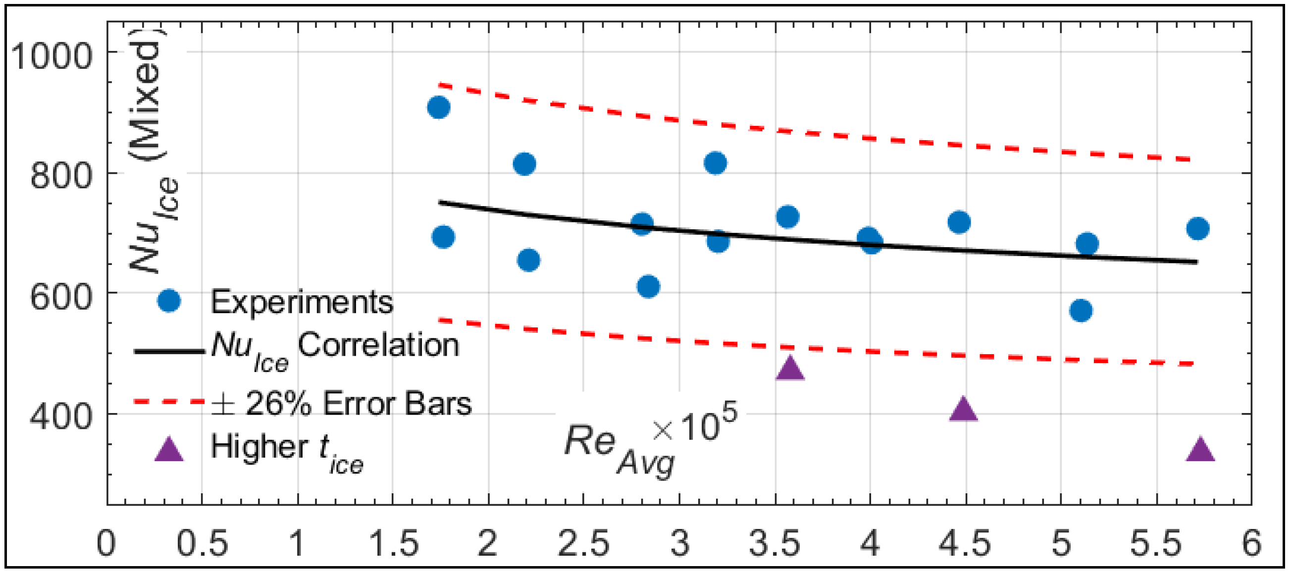
4.3. Correlations for the Nu_Ice

Finally, the correlation of the Nu_Ice with glaze ice was found to be in the form of Equation (12). Figure 22 shows the variation in the Nu_Ice versus Re_Avg for the glaze ice tests. In contrast to the Nu_Dry and the Nu_Wet, the Nu_Ice shows a decreasing behavior as the Re_Avg is increased. This is obvious with the negative m (m = −0.10) obtained in correlation (12). Almost all measured points lie within the ±26% error bars and the average error was approximately 4%.

The points that showed the maximum discrepancy with the correlation are displayed by the purple triangle. These points corresponded to the de-icing test# 9, where the t_ice at the tip was larger (7.99 mm) than the desired 6 mm. These points were not considered in data fitted for the correlation, although they lie withing the range of the experimental error.

$$N{u}_{Ice}\left(Glaze\right)=2.52\times {10}^3\times R{e}^{-0.10}\times {\mathrm{Pr}}^{1/3}$$

(12)

Similarly, Equation (13) is the result of correlating the data for the mixed glaze/rime ice tests. The correlation predictions and experimental values of the Nu_Ice versus Re_Avg is shown in Figure 23 but the fitting error was higher than the glaze ice tests at an average of 8.03%. Most points were within 26% of the correlation predictions, but again, the tests with the t_ice larger than 6 mm (test #15) showed the highest discrepancy from the correlation and are identified in Figure 23 by the purple triangles. These points lie outside the range of the experimental error and indicate that proposed correlation is sensitive to the ice layer on the blade.

$$N{u}_{Ice}\left(Mixed\right)=3.54\times {10}^3\times R{e}^{-0.12}\times {\mathrm{Pr}}^{1/3}$$

(13)

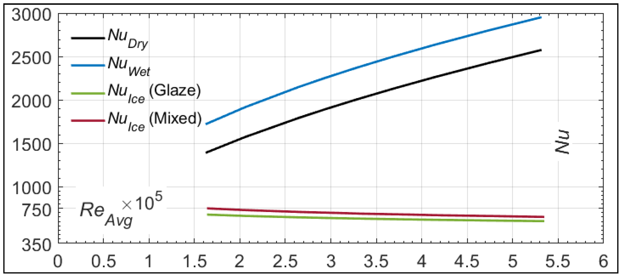
4.4. Comparison of Proposed Correlations

The proposed correlations are compared in Figure 24 that shows the variation in each versus the Re_Avg. The correlations reflect what is expected from the test setup as well as the findings of Section 0. The Nu_Wet correlation predicts values that are higher than that of the Nu_Dry. The increase in Nu due to the water spray is also reduced from 24% to 14% as the Re_Avg is increased. Similarly, the Nu_Ice correlation for mixed ice predicts values that are between 8% and 11% higher than that for glaze ice, which is also consistent with the findings of this work in Section 0.

5. Conclusions

This paper presented wind tunnel heat transfer measurements made at three different radial locations at the leading edge of a small 2-blade rotor. Rotor speeds of up to 1000 RPM were used with θ = 6°. The tests were run using both the anti-icing and de-icing modes. In the anti-icing tests, only water was impinging on the blades with no ice accumulation. In de-icing, an ice layer of approximately 6 mm was accreted near the tip of the blades before the heaters were turned on and ice was shed. The calculated Nu was analyzed for four specific conditions: first, the Nu_Dry with no water spray or ice on the blades; second, the Nu_Wet with water spray only; finally, the Nu_Ice, which represents heat transfer with an ice layer on the blade—once for glaze ice and another for mixed glaze/rime ice.

Results indicate that the Nu_Dry and the Nu_Wet directly increased with the increase in any of the three parameters: V_∝, r/R or Ω, mainly due to an increase in the Re. Compared to the Nu_Dry, the addition of water spray directly increased the heat transfer rates. The Nu_Wet to Nu_Dry ratio was more sensitive to Ω than to r/R or V_∝. As the Ω was increased, the ratio varied between 1.41 and almost 1 at the highest tested Ω. The increase in V_∝ caused both the Nu_Dry and the Nu_Wet to increase most at the smallest tested r/R, mainly due to the smaller velocity component due to rotation compared to the r/R near the tip of the blade. Nu_Ice behavior was different than that of the Nu_Dry and the Nu_Wet. The Nu_Ice was largely affected by the t_ice accreted on the blade. However, given similar test conditions and t_ice, the Nu_Ice decreased with r/R or Ω and increased with V_∝. Finally, the ice acted as insulation on the blade surface and the Nu_Ice to Nu_Dry ratio was always less than 1.

Four correlations are proposed based on the data gathered for the Nu_Dry, the Nu_Wet and the Nu_Ice, with an average error between 3.61% and 12.41%, thus providing a simplified approach to calculate heat transfer on the leading edge under icing conditions. The proposed Nu_Dry correlation agreed within 15.9% to a similar correlation near the leading edge of a fixed wing airfoil from the literature.

Future work includes expanding the tests to further investigate the effect of T_∝, LWC and t_ice on the proposed correlations. The A parameters of Equations (11)–(13) could then be expanded and include terms representing varying icing parameters (LWC or t_ice). Such studies would make heat transfer prediction more versatile and not only dependent on Re. The setup will also be modified to allow heating of the whole blade, preventing ice accumulation at the very end of the tip in the anti-icing mode.

References

1. Cao, Y.; Tan, W.; Wu, Z. Aircraft icing: An ongoing threat to aviation safety. Aerosp. Sci. Technol. 2018, 75, 353–385. [Google Scholar] [CrossRef]
2. Tarquini, S.; Antonini, C.; Amirfazli, A.; Marengo, M.; Palacios, J. Investigation of ice shedding properties of superhydrophobic coatings on helicopter blades. Cold Reg. Sci. Technol. 2014, 100, 50–58. [Google Scholar] [CrossRef]
3. SAE. Rotor Blade Electrothermal Ice Protection Design Considerations—Aerospace Standard AIR1667A; AC-9C Aircraft Icing Technology Committee: Warrendale, PA, USA, 2013. [Google Scholar]
4. Flemming, R. A History of Ice Protection System Development at Sikorsky Aircraft. In Proceedings of the FAA In-flight Icing/Ground De-icing International Conference & Exhibition, Chicago, IL, USA, 16–20 June 2003. [Google Scholar]
5. Aubert, R. History of Ice Protection System Design at Bell Helicopter. In Proceedings of the FAA In-flight Icing/Ground De-icing International Conference & Exhibition, Chicago, IL, USA, 16–20 June 2003. [Google Scholar]
6. Guffond, D. Icing and de-icing test on a 1/4 scale rotor in the ONERA S1MA wind tunnel. In Proceedings of the 24th Aerospace Sciences Meeting, Reno, NV, USA, 6–9 January 1986; p. 480. [Google Scholar]
7. Hanks, M.; Higgins, L.; Diekmann, V. Artificial and Natural Icing Tests Production UH-60A Helicopter; Army Aviation Engineering Flight Activity: Edwards AFB, CA, USA, 1980. [Google Scholar]
8. Leary, W.M. We Freeze to Please: A History of NASA’s Icing Research Tunnel and the Quest for Flight Safety; The NASA History Series; National Aeronautics and Space Administration NASA: Washington, DC, USA, 2002; Volume 4226. [Google Scholar]
9. Flemming, R.; Lednicer, D. Correlation of icing relationships with airfoil and rotorcraft icing data. J. Aircr. 1986, 23, 737–743. [Google Scholar] [CrossRef]
10. Miller, T.; Bond, T. Icing Research Tunnel Test of a Model Helicopter Rotor. In Proceedings of the 45th Annual Forum and Technology Display, Boston, MA, USA, 17–18 May 1989. [Google Scholar]
11. Britton, R.; Bond, T. A review of ice accretion data from a model rotor icing test and comparison with theory. In Proceedings of the 29th Aerospace Sciences Meeting, Reno, NV, USA, 7–10 January 1991; p. 661. [Google Scholar]
12. Flemming, R.; Bond, T.; Britton, R. Results of a Sub-Scale Model Rotor Icing Test. In Proceedings of the 29th Aerospace Sciences Meeting, Reno, NV, USA, 7–10 January 1991; p. 660. [Google Scholar]
13. Korkan, K. Experimental Study of Performance Degradation of a Rotating System in the NASA Lewis RC Icing Tunnel; Department of Aerospace Engineering, Texas A&M University: College Station, TX, USA, 1992. [Google Scholar]
14. Flemming, R.; Britton, R.; Bond, T. Model Rotor Icing Tests in the NASA Lewis Icing Research Tunnel. In Proceedings of the 68th Meeting of the Fluid Dynamic Panel Specialists Meeting on the Effects of Adverse Weather on Aerodynamics, Toulouse, France, 29 April–1 May 1991. [Google Scholar]
15. Bond, T.; Flemming, R.; Britton, R. Icing tests of a model main rotor. In Proceedings of the AHS 46th Annual Forum and Technology Display, Washington, DC, USA, 21–23 May 1990. [Google Scholar]
16. Thomas, S.K.; Cassoni, R.P.; MacArthur, C.D. Aircraft anti-icing and de-icing techniques and modeling. J. Aircr. 1996, 33, 841–854. [Google Scholar] [CrossRef]
17. Aliaga, C.N.; Aubé, M.S.; Baruzzi, G.S.; Habashi, W.G. FENSAP-ICE-Unsteady: Unified in-flight icing simulation methodology for aircraft, rotorcraft, and jet engines. J. Aircr. 2011, 48, 119–126. [Google Scholar] [CrossRef]
18. Han, Y.; Palacios, J. Transient heat transfer measurements of surface roughness due to ice accretion. In Proceedings of the 6th AIAA Atmospheric and Space Environments Conference, Atlanta, GA, USA, 16–20 June 2014; p. 2464. [Google Scholar]
19. Kreeger, R.E.; Tsao, J.-C. Ice Shapes on a Tail rotor. In Proceedings of the 6th AIAA Atmospheric and Space Environments Conference, Atlanta, GA, USA, 16–20 June 2014; p. 2612. [Google Scholar]
20. Wright, J.; Aubert, R. Icing wind tunnel test of a full scale heated tail rotor model. In Proceedings of the AHS 70th Annual Forum, Montreal, QC, Canada, 20–22 May 2014; pp. 20–22. [Google Scholar]
21. Tsao, J.-C.; Kreeger, R.E. Further Evaluation of Scaling Methods for Rotorcraft Icing; NASA Glenn Research Center: Cleveland, OH, USA, 2012. [Google Scholar]
22. Overmeyer, A.; Palacios, J.L.; Smith, E.C.; Royer, R. Rotating testing of a low-power, non-thermal ultrasonic de-icing system for helicopter rotor blades. In Proceedings of the SAE 2011 International Conference on Aircraft and Engine Icing and Ground Deicing, Chicago, IL, USA, 13–17 June 2011. [Google Scholar]
23. Reinert, T.; Flemming, R.J.; Narducci, R.; Aubert, R.J. Oscillating Airfoil Icing Tests in the NASA Glenn Research Center Icing Research Tunnel. In Proceedings of the SAE 2011 International Conference on Aircraft and Engine Icing and Ground Deicing, Chicago, IL, USA, 13–17 June 2011. [Google Scholar]
24. Han, Y.; Palacios, J.L.; Smith, E.C. An experimental correlation between rotor test and wind tunnel ice shapes on NACA 0012 airfoils. In Proceedings of the SAE 2011 International Conference on Aircraft and Engine Icing and Ground Deicing, Chicago, IL, USA, 13–17 June 2011. [Google Scholar]
25. Wang, Z.; Zhu, C.; Zhao, N. Experimental Study on the Effect of Different Parameters on Rotor Blade Icing in a Cold Chamber. Appl. Sci. 2020, 10, 5884. [Google Scholar] [CrossRef]
26. Fortin, G.; Perron, J. Spinning rotor blade tests in icing wind tunnel. In Proceedings of the 1st AIAA Atmospheric and Space Environments Conference, San Antonio, TX, USA, 22–25 June 2009; p. 4260. [Google Scholar]
27. Morency, F.; Tezok, F.; Paraschivoiu, I. Anti-icing system simulation using CANICE. J. Aircr. 1999, 36, 999–1006. [Google Scholar] [CrossRef]
28. Beaugendre, H.; Morency, F.; Habashi, W.G. FENSAP-ICE’s three-dimensional in-flight ice accretion module: ICE3D. J. Aircr. 2003, 40, 239–247. [Google Scholar] [CrossRef]
29. Beaugendre, H.; Morency, F.; Habashi, W.G. Development of a second generation in-flight icing simulation code. J. Fluids Eng. 2006, 128, 378–387. [Google Scholar] [CrossRef] [Green Version]
30. Reid, T.; Baruzzi, G.S.; Habashi, W.G. FENSAP-ICE: Unsteady conjugate heat transfer simulation of electrothermal de-icing. J. Aircr. 2012, 49, 1101–1109. [Google Scholar] [CrossRef]
31. Hannat, R.; Morency, F. Numerical validation of conjugate heat transfer method for anti-/de-icing piccolo system. J. Aircr. 2014, 51, 104–116. [Google Scholar] [CrossRef]
32. Pendenza, A.; Habashi, W.G.; Fossati, M. A 3D mesh deformation technique for irregular in-flight ice accretion. Int. J. Numer. Methods Fluids 2015, 79, 215–242. [Google Scholar] [CrossRef]
33. Pourbagian, M.; Habashi, W.G. Aero-thermal optimization of in-flight electro-thermal ice protection systems in transient de-icing mode. Int. J. Heat Fluid Flow 2015, 54, 167–182. [Google Scholar] [CrossRef]
34. Mu, Z.; Lin, G.; Shen, X.; Bu, X.; Zhou, Y. Numerical simulation of unsteady conjugate heat transfer of electrothermal deicing process. Int. J. Aerosp. Eng. 2018, 2018, 5362541. [Google Scholar] [CrossRef]
35. Narducci, R.; Kreeger, R.E. Analysis of a Hovering Rotor in Icing Conditions; NASA: Phoenix, AZ, USA, 2012. [Google Scholar]
36. Narducci, R.; Kreeger, R.E. Application of a High-Fidelity Icing Analysis Method to a Model-Scale Rotor in Forward Flight; NASA: Virginia Beach, VA, USA, 2012. [Google Scholar]
37. Chen, L.; Zhang, Y.; Wu, Q.; Chen, Z.; Peng, Y. Numerical Simulation and Optimization Analysis of Anti-/De-Icing Component of Helicopter Rotor Based on Big Data Analytics. In Methodology, Tools and Applications for Modeling and Simulation of Complex Systems, Proceedings of the AsiaSim 2016, SCS AutumnSim 2016, Beijing, China, 8–11 October 2016; Springer: Singapore, 2016; pp. 585–601. [Google Scholar]
38. Xi, C.; Qi-Jun, Z. Numerical simulations for ice accretion on rotors using new three-dimensional icing model. J. Aircr. 2017, 54, 1428–1442. [Google Scholar] [CrossRef]
39. Aubert, R. Additional Considerations for Analytical Modeling of Rotor Blade Ice. In Proceedings of the SAE 2015 International Conference on Icing of Aircraft, Engines, and Structures, Prague, Czech Republic, 22–25 June 2015. [Google Scholar]
40. Samad, A.; Tagawa, G.; Morency, F.; Volat, C. Predicting Rotor Heat Transfer Using the Viscous Blade Element Momentum Theory and Unsteady Vortex Lattice Method. J. Aerosp. 2020, 7, 90. [Google Scholar] [CrossRef]
41. Incropera, F.P.; Lavine, A.S.; Bergman, T.L.; DeWitt, D.P. Fundamentals of Heat and Mass Transfer, 7th ed.; John Wiley & Sons: New York, NY, USA, 2007. [Google Scholar]
42. Kays, W.M.; Crawford, M. Convective Heat and Mass Transfer, 3rd ed.; McGraw-Hill: New York, NY, USA, 1993. [Google Scholar]
43. Poinsatte, P.; Newton, J.; De Witt, K.; Van Fossen, J. Heat transfer measurements from a smooth NACA 0012 airfoil. J. Aircr. 1991, 28, 892–898. [Google Scholar] [CrossRef]
44. Henry, R.C.; Guffond, D.; Garnier, F.; Bouveret, A. Heat transfer coefficient measurement on iced airfoil in small icing wind tunnel. J. Thermophys. Heat Transf. 2000, 14, 348–354. [Google Scholar] [CrossRef]
45. Dukhan, N.; De Witt, K.J.; Masiulaniec, K.; Van Fossen, G.J., Jr. Experimental Frossling numbers for ice-roughened NACA 0012 airfoils. J. Aircr. 2003, 40, 1161–1167. [Google Scholar] [CrossRef]
46. Wang, X.; Naterer, G.; Bibeau, E. Experimental correlation of forced convection heat transfer from a NACA airfoil. Exp. Therm. Fluid Sci. 2007, 31, 1073–1082. [Google Scholar] [CrossRef]
47. Wang, X.; Naterer, G.; Bibeau, E. Convective heat transfer from a NACA airfoil at varying angles of attack. J. Thermophys. Heat Transf. 2008, 22, 457–463. [Google Scholar] [CrossRef]
48. Wang, X.; Naterer, G.; Bibeau, E. Convective droplet impact and heat transfer from a NACA airfoil. J. Thermophys. Heat Transf. 2007, 21, 536–542. [Google Scholar] [CrossRef]
49. Wang, X.; Naterer, G.; Bibeau, E. Multiphase Nusselt Correlation for the Impinging Droplet Heat Flux from a NACA Airfoil. J. Thermophys. Heat Transf. 2008, 22, 219–226. [Google Scholar] [CrossRef]
50. SAE. Calibration and Acceptance of Icing Wind Tunnels—Aerospace Standard ARP5905; AC-9C Aircraft Icing Technology Committee: Warrendale, PA, USA, 2003. [Google Scholar]
51. SAE. Droplet Sizing Instrumentation Used in Icing Facilities—Aerospace Standard AIR4906; AC-9C Aircraft Icing Technology Committee: Warrendale, PA, USA, 1995. [Google Scholar]
52. Samad, A.; Villeneuve, E.; Morency, F.; Volat, C. A Numerical and Experimental Investigation of the Convective Heat Transfer on a Small Helicopter Rotor Test Setup. J. Aerosp. 2021, 8, 53. [Google Scholar] [CrossRef]
53. IEC Corporation—Slip Ring Assemblies. Flange Mount Slip Ring. Available online: https://ieccorporation.com/flange-mount/ (accessed on 23 December 2020).
54. Eckert, E. Engineering relations for heat transfer and friction in high-velocity laminar and turbulent boundary-layer flow over surfaces with constant pressure and temperature. Trans. ASME 1956, 78, 1273–1283. [Google Scholar]
55. Moffat, R.J. Describing the uncertainties in experimental results. Exp. Therm. Fluid Sci. 1988, 1, 3–17. [Google Scholar] [CrossRef] [Green Version]
56. Li, G.; Gutmark, E.J.; Ruggeri, R.T.; Mabe, J. Heat Transfer and Pressure Measurements on a Thick Airfoil. J. Aircr. 2009, 46, 2130–2138. [Google Scholar] [CrossRef]
Figure 1. Icing Wind Tunnel.
Aerospace 08 00096 g001
Figure 2. Sprinkler Ramp.
Aerospace 08 00096 g002
Figure 3. Sketch with Dimensions of Blade and Heating Element: (a) Top View and (b) Side View.
Aerospace 08 00096 g003
Figure 4. Rotor Prototype in Wind Tunnel after a De-Icing Test.
Aerospace 08 00096 g004
Figure 5. A Photo of the Result of Anti-Icing Tests When the Ice Began to Accrete on the Previously Ice-Free Leading Edge Due to Gradual Reduction in Power Applied to the Activated Heaters; Ice Is Additionally Seen behind the Leading Edge and on the Blade Tip.
Aerospace 08 00096 g005
Figure 6. Instantaneous Variation in the Nu(t) for the Anti-Icing Test at T = 265.65 K for Ω = 500 RPM and V = 20 m/s (Test #9).
Aerospace 08 00096 g006
Figure 7. Photos of the De-Icing Test Process, (a) Ice Layer Accumulated across the Radius and on the Leading Edge of Blade (Top) and (b) Blade after Heating and Ice Totally Shed (Bottom).
Aerospace 08 00096 g007
Figure 8. Instantaneous Variation in the Nu(t) for the De-Icing Test at T = 265.65 K for Ω = 1000 RPM and V = 20 m/s (Test #9).
Aerospace 08 00096 g008
Figure 9. Variation in the Calculated NuDry with Respect to r/R for the Anti-Icing Tests at (a) V = 20 m/s and (b) V = 30 m/s.
Aerospace 08 00096 g009
Figure 10. Variation in the Calculated NuWet with Respect to r/R for the Anti-Icing Tests at (a) V = 20 m/s and (b) V = 30 m/s.
Aerospace 08 00096 g010
Figure 11. Ratios of the Calculated Nu between Tests at V = 30 m/s and V = 20 m/s for (a) the NuDry and (b) the NuWet.
Aerospace 08 00096 g011
Figure 12. Ratios of the Calculated NuWet to NuDry for the Anti-Icing Tests at (a) V = 20 m/s and (b) V = 30 m/s.
Aerospace 08 00096 g012
Figure 13. A Comparison between the Ice Types Obtained for Two Different Tests at Ω = 900 RPM and V = 20 m/s: (a) At T = 265.65 K: Glaze Ice that is Clear and Transparent and (b) At T = 258.15 K: Mixed Glaze/Rime Ice that is White and Opaque yet Slightly Transparent.
Aerospace 08 00096 g013
Figure 14. Variation in the Calculated NuIce with Respect to r/R for the De-Icing Tests with T ≈ 265.65 K and at (a) V = 20 m/s and (b) V = 30 m/s.
Aerospace 08 00096 g014
Figure 15. Variation in the Calculated NuIce with Respect to r/R for the De-Icing Tests with T ≈ 258.15 K and at (a) V = 20 m/s and (b) V = 30 m/s.
Aerospace 08 00096 g015
Figure 16. Ratios of the Calculated NuIce to the NuDry for the De-Icing Tests at T ≈ 265.65 K and (a) V = 20 m/s and (b) V = 30 m/s.
Aerospace 08 00096 g016
Figure 17. Ratios of the Calculated NuIce to NuDry for the De-Icing Tests at T ≈ 258.15 K and (a) V = 20 m/s and (b) V = 30 m/s.
Aerospace 08 00096 g017
Figure 18. Example of the Re Variation versus Time at the Three Blade Sections r/R = 0.6, 0.75 and 0.95 for the Anti-Icing Test #2 (Ω = 900 RPM and V = 20 m/s).
Aerospace 08 00096 g018
Figure 19. Comparison of the NuDry Correlation Predictions Versus Experimental Measurements of this Work.
Aerospace 08 00096 g019
Figure 20. Comparison of NuDry Correlation Predictions Versus Proposed Correlations from the Literature.
Aerospace 08 00096 g020
Figure 21. Comparison of Correlation Predictions versus Experimental Measurements for NuWet.
Aerospace 08 00096 g021
Figure 22. Comparison of Correlation Predictions versus Experimental Measurements of NuIce for the De-Icing Tests with Glaze Ice.
Aerospace 08 00096 g022
Figure 23. Comparison of Correlation Predictions Versus Experimental Measurements for the NuIce for the De-Icing Tests with Rime Ice.
Aerospace 08 00096 g023
Figure 24. A Comparison of the Correlation Predictions versus ReAvg for the NuDry and the NuWet as well as both types of NuIce.
Aerospace 08 00096 g024