\({\mathcal{L}_1}\) Adaptive Loss Fault Tolerance Control of Unmanned Hypersonic Aircraft with Elasticity

Abstract

This paper investigates the fault tolerance control of hypersonic aircrafts with ${\mathcal{L}}_1$ adaptive control method in the presence of loss of actuator effectiveness fault. The hypersonic model considers the uncertainties caused by the features of nonlinearities and couplings. Elasticity is taken into account in hypersonic vehicle modeling which makes the model more accurate. A velocity ${\mathcal{L}}_1$ adaptive controller and an altitude ${\mathcal{L}}_1$ adaptive controller are designed to control flexible hypersonic vehicle model with actuator loss fault. A PID controller is designed as well for comparison. Finally, the simulation results are used to analyze the effectiveness of the controller. Compared to the results of PID controller, ${\mathcal{L}}_1$ controllers have better performance.

1. Introduction

Hypersonic vehicles refer to aircrafts, missiles, artillery shells and other vehicles with or without wings that travel at more than five times the speed of sound. Characterized by high penetration rate, hypersonic vehicles have great potential value both in military and economy. X-51, the first flight with an air-breathing scramjet engine in America, is a milestone in the development of hypersonic vehicle [1]. A program named “Promethee” was launched in France to study hypersonic vehicles [2]. In Banalor, India has made great efforts to hypersonic aerodynamics [3]. And China has made huge progress in air-breathing systems in recent years [4]. Hypersonic vehicle, for its important application value in the military field, has arisen extensive attention from a number of countries [5]. It is of great importance to study the control of hypersonic vehicles.

Hypersonic vehicle is designed with complex stress conditions, and the applicability of mathematical model determines its control effect to a certain extent. In 2007, Parker put forward a control model of hypersonic vehicle [6], which was made intuitively by abstracting formulas from various stress conditions. Fiorentini made some improvements to Parker’s model [7]. In Fiorentini’s study, the model was further reduced to four formulas and some variables with little influence were omitted. However, both models are only applicable to rigid bodies. The high speed of hypersonic vehicle has certain influence on its elasticity. Zong put forward a hypersonic model that took elasticity into account [8]. Liu developed a more accurate elastic replacement model [9]. In the modeling, comprehensive algorithm [10], quantitative echo [11], two-stage orbit [12] and other new methods based on the BGK scheme of gas dynamics were adopted. Today, the modeling of hypersonic vehicle is still a heated issue.

Hypersonic vehicle plays an important role in aircraft application, so that its security must be guaranteed. If a hypersonic vehicle is working in a tough environment, more uncertainties and a greater chance of failure may occur. Tang studied the fault tolerance of full state constrains [13]. Sun studied methods for dealing with input saturation and state constraints [14]. Cheng focused on the breakdown and rebound of the actuator [15]. And An focused on the attack constraint [16]. There are many methods used for fault-tolerant control. Some traditional control methods, such as PID, can tolerate failures, but only applicable for simple systems. Some advanced methods, such as Barrier Lyapunov function based adaptive finite time control [17], second-class fuzzy technology and cuckoo search algorithm, have achieved good results in complex systems [18]. ${\mathcal{L}}_1$ adaptive control is usually not applied to fault-tolerant control, while ${\mathcal{L}}_1$ adaptive fault-tolerant control is usually applied to four-rotor vehicles, such as [19,20,21,22]. It is of great significance to apply ${\mathcal{L}}_1$ adaptive control in fault-tolerant control of hypersonic vehicles.

First, the hypersonic mathematical model is determined as a non-minimum phase flexible model in this paper. In order to simplify the structure of the controller and take the elastic model into consideration, a hypersonic model is established as a reference model [8]. The model contains not only elasticity but also uncertainty, so it is particularly important to study this model. As the modal frequency of aircraft structure is closer to the rigid modal frequency, the influence of elastic effect on the flight dynamics of elastic aircraft becomes increasingly significant. In particular, the processing and stability characteristics will become more complex and serious, and the "rigid aircraft" analysis method cannot be studied. Therefore, it is urgent to establish a multi-disciplinary coupling flight dynamics model of elastic vehicle. In this paper, the elastic engine model is taken as a part of the hypersonic vehicle model to make the mathematical model closer to the actual hypersonic vehicle dynamics. Second, the failure of the actuator is a loss failure. In reality, due to the wear and tear of the vehicle and the inherent age limit, loss failures often occur. Pneumatic rudder plays a decisive role in aircrafts, which is a guarantee to avoid loss failure. Proposed by Hovakimyan et al. in 2011, ${\mathcal{L}}_1$ adaptive control is a fast and robust adaptive control method as stated in [23]. By adding a low-pass filter to the control law design, the separation of control law from adaptive law design is ensured. According to the particularity of the supersonic aircraft model, the height controller needs to derive the relationship between control value and state by backstepping. Then, in this paper, the ${\mathcal{L}}_1$ adaptive control method is introduced to control the hypersonic vehicle with elasticity and loss fault. ${\mathcal{L}}_1$ adaptive fault-tolerance control is an active fault-tolerant control that readjusts the parameters of the controller according to the fault, and can deal with the fault actively. Besides, the adaptive fault tolerance of fault occurrence amplitude is superior to passive fault tolerance control. In order to improve the performance of the control system to a greater extent, traditional ${\mathcal{L}}_1$ adaptive control needs to combine with fault tolerance control.

Since we consider aeroelastic model in this paper, the generalized aeroelastic force will affect the force and torque of the hypersonic vehicle. It makes the whole system more likely to get into an unstable state and increases the difficulty of control. When the faults of actuators occur the control ability will reduce significantly and the impact of elasticity on the system stability will be intensified. Therefore, to improve reliability of the control system, fault-tolerant controller with rapid response is necessary for the elastic hypersonic vehicle. We propose a ${\mathcal{L}}_1$ adaptive fault-tolerant control method which combines the ${\mathcal{L}}_1$ adaptive control method and fault-tolerant control theory. Firstly, ${\mathcal{L}}_1$ adaptive control is a model following reconfiguration fault-tolerant control which does not require high linearity of the model and can be applied to nonlinear model like the hypersonic aircraft used in this paper. The internal structures of ${\mathcal{L}}_1$ adaptive methods vary with model. The states, disturbances and reference trajectory of hypersonic vehicles can all be considered in designing adaptive parameters of controller. So ${\mathcal{L}}_1$ adaptive control can have more targeted control effects for the specific aircraft. Secondly, as an improved method of ${\mathcal{L}}_1$ adaptive control, ${\mathcal{L}}_1$ adaptive fault-tolerance controller’s response speed is fast due to its structure of separating feedback control and adaptive law. For elastic hypersonic vehicle, the fast reaction rate is necessary. Besides that, it can also reduce the influence time of faults and improve flight quality. Finally, low-pass filters are designed to add into ${\mathcal{L}}_1$ adaptive fault-tolerant controllers to restrain high frequency oscillation of control inputs. It can avoid the irreversible results produced by the interaction of high-frequency oscillation and aeroelasticity.

The paper is organized as follows. First, the dynamic model of the hypersonic aircraft is built in Section 2. Then, the ${\mathcal{L}}_1$ adaptive controller is designed and the stability is proved in Section 3. In Section 4, the simulation results are shown and analyzed. Finally, conclusion of the whole paper is present in Section 5.

The main contributions of this paper can be highlighted as follows.

(a) We build a hypersonic aircrafts model with loss fault and take elasticity into account. We simplify the model to a control-oriented model.

(b) We investigate the combination method of ${\mathcal{L}}_1$ adaptive control and fault tolerance control. We propose two kinds of combination methods to suit different aircraft modeling situations.

(c) We apply ${\mathcal{L}}_1$ adaptive fault tolerance control method to hypersonic aircraft model and keep the hypersonic aircraft with elasticity tracking the reference longitudinal velocity and altitude in loss fault situations which have better performance than PID controller.

2. Problem Formulation

2.1. Dynamic Motion Equations

Assuming that the earth is flat, the earth coordinate system is chosen as the inertial seat. The frame beam is a free beam structure at both ends, and the first three elastic modes are considered. In [7], a model of rigid-body vehicle dynamics is proposed.

Table 1. Explanation of Parameters.

Parameter	Explanation	Parameter	Explanation
m	mass	$\overline{q}$	dynamic pressure
V	velocity	$\rho$	air density
h	altitude	${\rho }_0$	air density at nominal altitude
$\gamma$	track angle	$h_0$	nominal altitude
$\theta$	pitch angle	$h_s$	inverse of the air density exponential decay rate
Q	pitch angle rate	$N_i$	generalized force
$\alpha$	attack angle	${\eta }_i$ and ${\dot{\eta }}_i$	six elastic states
T	thrust	${\zeta }_i$	damping factor
D	drag	${\omega }_i$	natural oscillation frequency
L	lift	n	loss rate
M	pitching torque	${\gamma }_r$	reference pitch angle
g	acceleration due to gravity	${\varpi }_i(i=V,\gamma ,Q)$	uncertainties
$I_{yy}$	moment of inertia along the longitudinal direction	${\widehat{\theta }}^T\left(t\right)$	adaptive variable
$\varphi$	fuel equivalent ratio	$K_V$	velocity gain
${\delta }_e$	elevator deflection angle	${\varsigma }_V$	control law
$\overline{c}$	mean aerodynamic chord	$K_i(i=1,2)$	adaption gain
S	reference area	$P_i(i=1,2)$	the solution of Lyapunov equation
$z_T$	thrust-to-moment coupling coefficient	$D_1\left(s\right)(i=1,2)$	low-filter

lists the meanings of each parameter appearing in the model.

Consider the decoupled longitudinal dynamic merely, the longitudinal rigid-body can be written as:

$$\begin{array}{c}m\dot{V}=Tcos\alpha -D-mgsin\gamma \hfill \\ \dot{h}=Vsin\gamma \hfill \\ \dot{\gamma }=\frac{L+Tsin\alpha }{mV}-\frac{g}{V}cos\gamma ,\hfill \\ \dot{\theta }=Q\hfill \\ I_{yy}\dot{Q}=M\hfill \end{array}$$

(1)

where m is mass, V, h, $\gamma$, $\theta$ and Q denote five rigid body states of the system, named velocity, altitude, track angle, pitch angle and pitch angle rate, $\alpha =\theta -\gamma$ is attack angle, T, D, L, M present thrust, drag, lift and pitching torque, g is acceleration due to gravity, $I_{yy}$ denotes moment of inertia along the longitudinal direction.

In Equation (1), the forces and the torques are calculated as follow:

$$\begin{array}{c}T=\overline{q}S(C_T+{C_T}^{\varphi }\varphi +{C_T}^{\eta }\eta )\hfill \\ D=\overline{q}S(C_D+{C_D}^{{{\delta }_e}^2}{{\delta }_e}^2+{C_D}^{{\delta }_e}{\delta }_e+{C_D}^{\eta }\eta ),\hfill \\ L=\overline{q}S(C_L+{C_L}^{{\delta }_e}{\delta }_e+{C_L}^{\eta }\eta )\hfill \\ M=\overline{q}\overline{c}S(C_M+{C_M}^{{\delta }_e}{\delta }_e+{C_M}^{\eta }\eta )+z_{T}T\hfill \end{array}$$

(2)

where $\varphi$ and ${\delta }_e$ are control inputs, respectively fuel equivalent ratio and elevator deflection angle, $\overline{c}$ is mean aerodynamic chord, S presents the reference area, $z_T$ denotes the thrust-to-moment coupling coefficient, $\overline{q}$ is dynamic pressure and expressed as:

$$\overline{q}=\frac{\rho V^2}{2}=\frac{{\rho }_0{e}^{-(h-h_0)/h_s}{V}^2}{2},$$

(3)

where $\rho$ is air density, ${\rho }_0$ is air density at nominal altitude, $h_0$ presents nominal altitude and $h_s$ denotes inverse of the air density exponential decay rate. Other coefficients $C_T$, ${C_T}^{\varphi }$, $C_D$, $C_L$, $C_M$ are given by:

$$\begin{array}{c}{C}_T={C_T}^{{\alpha }^3}{\alpha }^3+{C_T}^{{\alpha }^2}{\alpha }^2+{C_T}^{\alpha }\alpha +{C_T}^0\hfill \\ {C_T}^{\varphi }={C_T}^{\varphi {\alpha }^3}{\alpha }^3+{C_T}^{\varphi {\alpha }^2}{\alpha }^2+{C_T}^{\varphi \alpha }\alpha +{C_T}^{\varphi 0}\hfill \\ C_D={C_D}^{{\alpha }^2}{\alpha }^2+{C_D}^{\alpha }\alpha +{C_D}^0,\hfill \\ C_L={C_L}^{\alpha }\alpha +{C_L}^0\hfill \\ C_M={C_M}^{{\alpha }^2}{\alpha }^2+{C_M}^{\alpha }\alpha +{C_M}^0\hfill \end{array}$$

(4)

For hypersonic vehicles, rigid-body dynamic model can not analogy the real dynamic situation of hypersonic vehicles. In order to obtain a more accurate result, the elasticity of hypersonic vehicles must be considered. The flexible engine model of air-breathing hypersonic aircraft with non-minimum phase shown in [8] is presented as follow:

$${\ddot{\eta }}_i=-2{\zeta }_i{\omega }_i{\dot{\eta }}_i-{{\omega }_i}^2{\eta }_i+N_i(i=1,2,3),$$

(5)

where $N_i$ present generalized force, ${\eta }_i$ and ${\dot{\eta }}_i$ present six elastic states, ${\zeta }_i$ is the damping factor, ${\omega }_i$ is the natural oscillation frequency. In Equation (5), the forces and the torques are calculated as follow:

$$\begin{array}{c}{N}_i=\overline{q}S({N_i}^{{\alpha }^2}{\alpha }^2+{N_i}^{\alpha }\alpha +{N_i}^{{\delta }_e}{\delta }_e+{N_i}^{\eta }\eta +{N_i}^0)\\ (i=1,2,3)\\ {K_j}^{\eta }=[{K_j}^{{\eta }_1},{K_j}^{{\eta }_2},{K_j}^{{\eta }_3}]\\ (K=C,N;j=T,D,L,M).\end{array}$$

(6)

The elasticity of hypersonic vehicles is relate to the attack angle. When hypersonic vehicle takes large maneuver, the elasticity makes great influence on stress situation. The model of hypersonic vehicle model becomes more accurate but more difficult to control.

According to Equation (2), it can be seen that the coupling between elevator and lift affects the track angle, which causes a problem that the control law of elevator derived by standard inversion method based on the dynamics of altitude h and track angle $\gamma$ makes the internal dynamic pitch angle and pitch angular velocity unstable. In order to solve this problem, the elevator deflection angle ${\delta }_e$ in the track angle $\gamma$ is regarded as uncertainty so that the effect of ${\delta }_e$ on altitude only appears in pitch angular velocity and the correlation of h is improved. In addition, all items except pitch angle $\theta$ are considered as uncertainties in the track angle formula. Besides, in order to decouple the longitudinal velocity and height in the controller, we consider the ${\delta }_e$ in the longitudinal speed as uncertainty and ignore the effect of fuel equivalent in pitch angular velocity. Finally, the control oriented model is obtained by simplifying the model, which is written in the form of the sum of constant, control quantity and uncertainty in Equation (7). The longitudinal velocity control logic can be set as fuel equivalent ratio-longitudinal thrust-longitudinal velocity and the altitude control logic is elevator deflection angle-pitching moment-pitch angular velocity-pitching angle-track angle-altitude.

2.2. Loss Fault and Model Simplification

For hypersonic aircrafts, when there’s a loss fault, it always comes to the pneumatic rudder. Specific to this paper, it is elevator deflection. Reflected on the model, it is a loss rate n acting on ${\delta }_e$. According to Equations (1)–(4), each state is influenced by elevator deflection angle. It will cause plenty of extra calculation and deform the control effect if n is multiplied directly.

Treat ${\delta }_e$ as an uncertainty in V, ignore others except $\theta$ in $\dot{\gamma }$ and treat $\varphi$ an uncertainty in Q as well. The model shown as Equation (1) can be simplified as:

$$\begin{array}{c}\dot{V}=\frac{\overline{q}S(C_{T}cos\alpha -C_D)-mgsin\gamma }{m}+\frac{\overline{q}S{C_T}^{\varphi }cos\alpha }{m}\varphi +{\varpi }_V\hfill \\ =V_0+V_c\varphi +{\varpi }_V\hfill \\ \dot{h}=Vsin\gamma \hfill \\ {\dot{\gamma }}_e=\theta +{\varpi }_{\gamma },\hfill \\ \dot{\theta }=Q\hfill \\ \dot{Q}=\frac{z_T\overline{q}S{C}_T+\overline{q}\overline{c}S{C}_M}{I_{yy}}+\frac{\overline{q}\overline{c}S{C_M}^{{\delta }_e}}{I_{yy}}n{\delta }_e+{\varpi }_Q\hfill \\ =Q_0+Q_{c}n{\delta }_e+{\varpi }_Q\hfill \end{array}$$

(7)

where ${\gamma }_e=\gamma -{\gamma }_r$, ${\gamma }_r$ is the reference pitch angle and ${\varpi }_i(i=V,\gamma ,Q)$ present uncertainties. Although the control right is sacrificed after simplification, the designs of controllers become more convenient and increase the speed of fault tolerance control.

In aircraft control, the selected control variables are variables of actuator such as rudder deflection, motor speed, etc. or the variables that have operation relationship with the actuator such as force and torque. The fault mode selected in this paper is the loss fault acting on the actuator which makes the control value reduced in the simulation part. Then, the goal of fault tolerance control is to ensure that the final output control value is close to the output value of the fault-free state. The main methods are as follows:

1. Use the fault-tolerant ability of ${\mathcal{L}}_1$ adaptive controller

In the formula $u\left(t\right)={\widehat{\theta }}^T\left(t\right)x\left(t\right)+k_{g}r\left(t\right)$, ${\widehat{\theta }}^T\left(t\right)$ is an adaptive variable which is adjusted according to the error of the return controller outputs. When there is no fault in the actuator, the adaptive variable is affected by the error. In order to make the controller fault-tolerant, fault information is added into the adaptive variable to make it follow the fault of the actuator. The corresponding increase or decrease is made to ensure that the final control value remains unchanged. This method is suitable for the system whose control variable is the actuator variable and the system with simple structure.

2. Add compensators to the designed controller

Make the control quantity output under the non-fault state into the ideal control quantity. Under the loss fault condition, the ideal control quantity can be written as the sum of the failure control quantity and the compensation quantity. Then, in the process of modeling, the sum of failure control value and the compensation value can represent the ideal control quantity all the time. So the compensation value becomes a part of the control quantity with the design of the controller. This method is suitable for the system whose control variables are not actuator variables. Only a part of the control variables in this system are affected by the fault, and only the part responding to the fault needs to be fault tolerant.

3. ${\mathcal{L}}_{\mathbf{1}}$ Adaptive Controller Design

It should be noted that the italic style of ${\mathcal{L}}_1$ here is a special symbol.

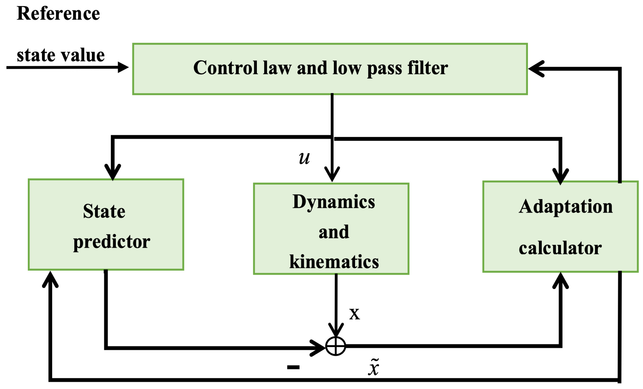
Figure 1 shows the internal structure of ${\mathcal{L}}_1$ adaptive controller, it consists of four parts: control law, state predictor, adaption part and kinematics and dynamics. The part of control law outputs the control values to other three parts. Adaption part is influenced by the difference of state predictor and force model and outcomes adaptive quantities to control law and state predictor.

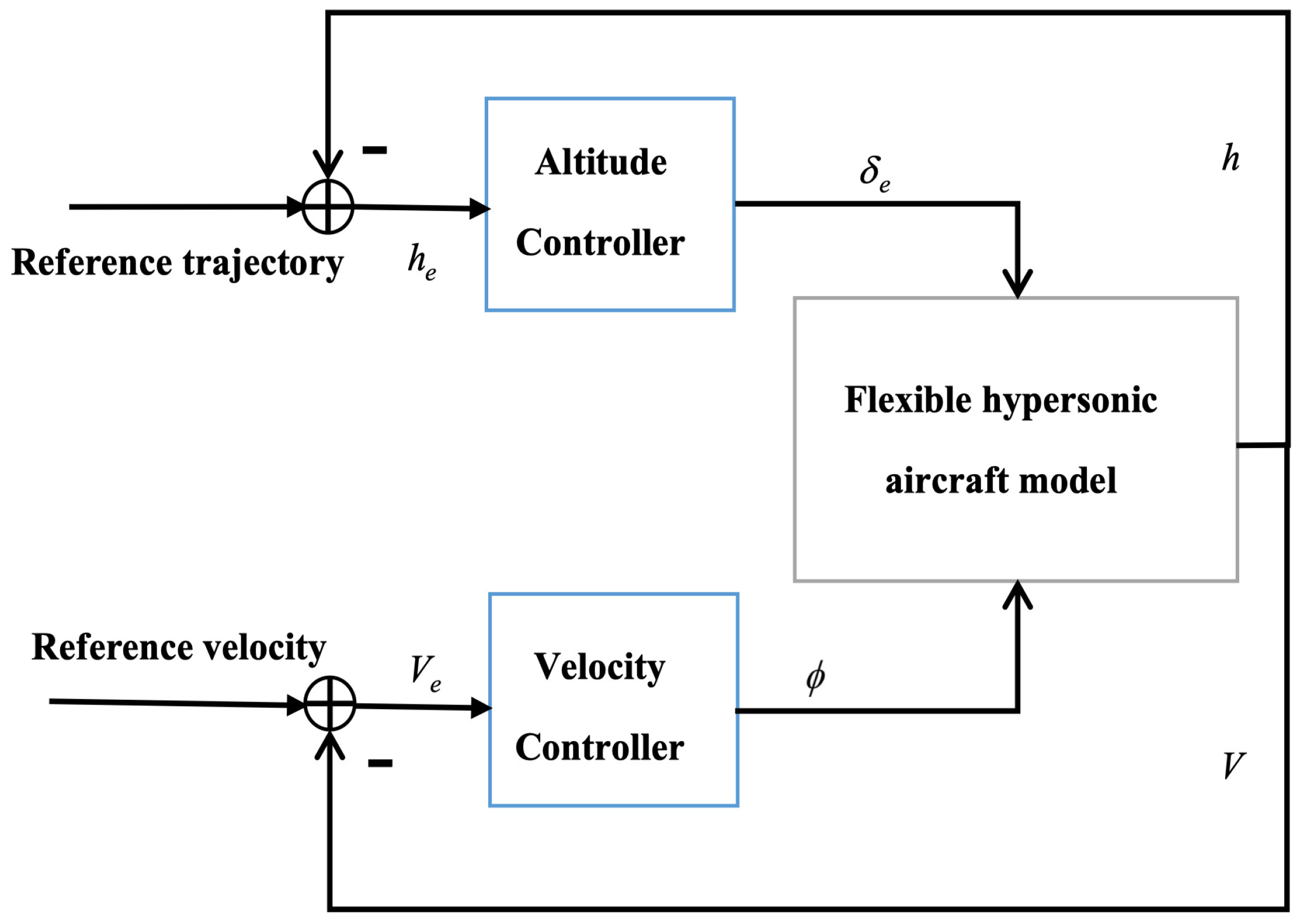
As illustrated in Figure 2, there are two ${\mathcal{L}}_1$ controllers in the control system. One is used to control velocity and the other is altitude controller. The reference altitude and longitudinal velocity are designed in advance and two controllers accept real state value from the aircraft model. Fuel equivalent ratio and elevator deflection angle are output to flexible hypersonic model.

3.1. Velocity Controller

The velocity error dynamic is defined as follows:

$${\dot{V}}_e=\dot{V}-{\dot{V}}_r=V_0+V_c\varphi +{\varpi }_V-{\dot{V}}_r.$$

(8)

Define the control value as $u_V=\varphi$ and design the control input $\varphi$:

$$\varphi =-K_V{V}_e-V_0+{\dot{V}}_r+{\varsigma }_V,$$

(9)

$K_V$ is the velocity gain and ${\varsigma }_V$ is the control law needed to be design. Equation (8) can be written as follow:

$$\begin{array}{c}{\dot{V}}_e=V_0+V_c\varphi +{\varpi }_V-{\dot{V}}_r\hfill \\ =-K_V{V}_e+(V_c-1)\varphi +{\varpi }_V+{\varsigma }_V,\hfill \\ =-K_V{V}_e+{\sigma }_1\varphi +{\varpi }_V+{\varsigma }_V\hfill \end{array}$$

(10)

where ${\sigma }_1=V_c-1$ which is bounded and satisfies $\left|{\sigma }_1\right|\le {\kappa }_1$ and ${\varpi }_V$ satisfied $|{\varpi }_V|\le {\mu }_1$. The state of velocity control is $x_1=V_e$ and the control system can be described as:

$$\begin{array}{c}{\dot{x}}_1=A_1{x}_1+b_1({\sigma }_1\varphi +{\varpi }_V+{\varsigma }_V),\\ y_1=c_1{x}_1\end{array}$$

(11)

where $A_1=-K_V$, $b_1=1$ and $c_1=1$. The state predictor subsystem of velocity is presented as:

$$\dot{\widehat{}}{x}_1=A_1{\widehat{x}}_1+b_1({\widehat{\sigma }}_1\varphi +{\widehat{\varpi }}_V+{\varsigma }_V),$$

(12)

where ${\widehat{\sigma }}_1$ and ${\widehat{\varpi }}_V$ are given by projection operator and have the same boundaries as ${\sigma }_1$ and ${\varpi }_V$ respectively:

$$\begin{array}{c}{\dot{\widehat{}}\sigma }_1=K_{1}proj({\widehat{\sigma }}_1,-b_1\varphi P_1{\tilde{x}}_1).\hfill \\ {\dot{\widehat{}}\varpi }_V=K_{1}proj({\widehat{\varpi }}_V,-b_1{P}_1{\tilde{x}}_1)\hfill \end{array}$$

(13)

In Equation (13), ${\tilde{x}}_1={\widehat{x}}_1-x_1$, $K_1$ is the adaption gain and $P_1$ is the solution of Lyapunov equation ${A_1}^T{P}_1+P_1{A}_1=-Q_1$, where $Q_1>0$ is known. The control law is defined as follow:

$${\varsigma }_V\left(s\right)=D_1\left(s\right){\chi }_1\left(s\right),$$

(14)

$D_1\left(s\right)$ is a low-filter needed to be chosen. The ${\chi }_1\left(s\right)$ is laplace transformed from:

$${\chi }_1\left(t\right)=-{\widehat{\sigma }}_1\varphi -{\widehat{\varpi }}_V.$$

(15)

Definition 1.

For a n×m-dimensional output system $G\left(s\right)$, its ${\mathcal{L}}_1$ norm is defined as ${∥G\left(s\right)∥}_{L_1}={max}_{i=1,2,\Vert ,n}\left({\displaystyle \sum _{j=1}^m}{∥G_{ij}\left(s\right)∥}_{L_1}\right)$, where $G_{ij}\left(s\right)$ is the element of row i and column j.

Lemma 1.

For a stable MIMO system, if the input is $u\left(t\right)$ and the output is $y\left(t\right)$, then ${∥y\left(t\right)∥}_{L_{\infty }}\le {∥G\left(s\right)∥}_{L_1}{∥u\left(t\right)∥}_{L_{\infty }}$ where ${∥u\left(t\right)∥}_{L_{\infty }}=max\left(y\left(t\right)\right)$.

Corollary 1.

For a stable MIMO system, if the input is bounded, then the output is bounded as well which means $max\left(y\right(t\left)\right)$ is bounded.

Lemma 2.

For series system $G\left(s\right)=G_1\left(s\right)G_2\left(s\right)$, $G_1\left(s\right)\in \mathbb{R}{}^{n\times l}$, $G_2\left(s\right)\in \mathbb{R}{}^{l\times m}$, there is ${∥G\left(s\right)∥}_{L_1}\le {∥G_1\left(s\right)∥}_{L_1}{∥G_2\left(s\right)∥}_{L_1}$.

Theorem 1.

(${\mathcal{L}}_1$ small gain theorem): For a system with input $u\left(t\right)$ and output $y\left(t\right)$: $y\left(t\right)=N_1\left(s\right)(u\left(t\right)-N_2\left(s\right)y\left(t\right))$, where $N_1\left(s\right)$ is the transfer function of forward path and $N_2\left(s\right)$ is the transfer function of feedback loop. If ${∥N_1\left(s\right)∥}_{L_1}{∥N_2\left(s\right)∥}_{L_1}<1$, then the system is asymptotically stable.

Lemma 3.

If $A\in \mathbb{R}{}^{n\times n}$, $b\in \mathbb{R}{}^{n\times 1}$ is controllable, the matrix N is full rank.

Lemma 4.

If $A\in \mathbb{R}{}^{n\times n}$, $b\in \mathbb{R}{}^{n\times 1}$ is controllable and ${(sI-A)}^{-1}b$ is asymptotically stable, there is a matrix $c\in \mathbb{R}{}^{1\times n}$ which enables $c{(sI-A)}^{-1}b$ become the minimum phase system with relativity of 1.

Proof. 

By changing the low-filter $D_1\left(s\right)$ to satisfy the ${\mathcal{L}}_1$-norm stability condition, just ensure the Lyapunov function is negative definite, the control system is stable and according to Theorem 1 the system satisfies:

$${∥G_1\left(s\right)∥}_{L_1}{∥\sigma ∥}_{L_1}<1,$$

(16)

where $G_1\left(s\right)={(s-A_1)}^{-1}{b}_1(1-D_1\left(s\right))$. The Lyapunov function is defined as follow:

$$E_V=P_1{{\tilde{x}}_1}^2+{K_1}^{-1}{{\tilde{\sigma }}_1}^2+{K_1}^{-1}{{\tilde{\varpi }}_V}^2,$$

(17)

where ${\tilde{\sigma }}_1={\widehat{\sigma }}_1-{\sigma }_1$, ${\tilde{\varpi }}_V={\widehat{\varpi }}_V-{\varpi }_V$. The derivative of $E_V$ can be written as:

$$\begin{array}{c}{\dot{E}}_V=2P_1{\dot{\tilde{}}x}_1{\tilde{x}}_1+2{K_1}^{-1}{\dot{\tilde{}}\sigma }_1{\tilde{\sigma }}_1+2{K_1}^{-1}{\dot{\tilde{}}\varpi }_V{\tilde{\varpi }}_V\hfill \\ =2P_1(A_1{\tilde{x}}_1+b_1{\tilde{\sigma }}_1\varphi ){\tilde{x}}_1-2{K_1}^{-1}{\tilde{\varpi }}_V{\dot{\varpi }}_V\hfill \\ +2{K_1}^{-1}{\tilde{\varpi }}_V({\dot{\widehat{}}\varpi }_V+K_1{b}_1{P}_1{\tilde{x}}_1)\hfill \\ +2{K_1}^{-1}{\tilde{\sigma }}_1({\dot{\widehat{}}\sigma }_1+K_1{b}_1{u}_V{P}_1{\tilde{x}}_1)\hfill \\ \le -Q_1{{\tilde{x}}_1}^2-2{K_1}^{-1}{\tilde{\varpi }}_V{\dot{\varpi }}_V\hfill \\ \le -Q_1{{\tilde{x}}_1}^2+2{K_1}^{-1}\left|{\tilde{\varpi }}_V{\dot{\varpi }}_V\right|.\hfill \end{array}$$

(18)

 □

Let ${\varpi }_V$ be continuously differentiable with uniformly bounded derivaties ${\varpi }_{V1}$, so we can obtain $|{\tilde{\varpi }}_V^T{\dot{\varpi }}_V|\le 2{\mu }_1{\varpi }_{V1}$ and then ${\dot{E}}_V\le -{\tilde{x}}_1^T{Q}_1{\tilde{x}}_1+4{K_1}^{-1}{\mu }_1{\varpi }_{V1}$.

Define a constant:

$${\mathsf{\Xi }}_1\stackrel{\mathsf{\Delta }}{=}4\frac{{\lambda }_{max}\left(P_1\right)}{{\lambda }_{min}\left(Q_1\right)}{\mu }_1{\varpi }_{V1}+4\left(max|{\sigma }_1{|}^2+{{\mu }_1}^2\right).$$

(19)

First, assume there exists $t_1>0$ and $E_V\left(t_1\right)>{K_1}^{-1}{\mathsf{\Xi }}_1$. Because $max{K_1}^{-1}({\tilde{\sigma }}_1^T{\tilde{\sigma }}_1+{\tilde{\varpi }}_V^T{\tilde{\varpi }}_V)\le 4{K_1}^{-1}\left(max|{\sigma }_1{|}^2+{{\mu }_1}^2\right)$, it follows from Equation (17) that

$$P_1{{\tilde{x}}_1}^2\ge 4{K_1}^{-1}\frac{{\lambda }_{max}\left(P_1\right)}{{\lambda }_{min}\left(Q_1\right)}{\mu }_1{\varpi }_{V1},$$

(20)

and

$$Q_1{{\tilde{x}}_1}^2\ge P_1{{\tilde{x}}_1}^2\frac{{\lambda }_{min}\left(Q_1\right)}{{\lambda }_{max}\left(P_1\right)}=4{K_1}^{-1}{\mu }_1{\varpi }_{V1}.$$

(21)

So it can be obtained that when $E_V\left(t\right)>{K_1}^{-1}{\mathsf{\Xi }}_1$ ($K_1$ is always above 1),

$$\begin{array}{c}{\dot{E}}_V\le -Q_1{{\tilde{x}}_1}^2+2{K_1}^{-1}\left|{{\tilde{\varpi }}_V}^T{\dot{\varpi }}_V\right|\hfill \\ \le -4{K_1}^{-1}{\mu }_1{\varpi }_{V1}+4{\mu }_1{\varpi }_{V1}\le 0.\hfill \end{array}$$

(22)

Then assume $t_1\ge 0$, $E_V\left(t\right)\le {K_1}^{-1}{\mathsf{\Xi }}_1$, we obtain $P_1{{\tilde{x}}_1}^2\le E_V\le {K_1}^{-1}{\mathsf{\Xi }}_1$. Since

$${\lambda }_{min}\left(P_1\right){∥{\tilde{x}}_1∥}_2\le P_1{{\tilde{x}}_1}^2,$$

(23)

there is

$${∥{\tilde{x}}_1∥}_{L_{\infty }}\le \sqrt{\frac{{\mathsf{\Xi }}_1}{{\lambda }_{min}\left(P_1\right)K_1}},$$

(24)

the velocity control system is stable.

3.2. Altitude Controller

By combining the last four formulas in Equation (1) with small angle approximation, the altitude dynamic can be obtained. ${\delta }_e$ does not have direct relation with h, so it has to set up the relationship from the twice formula to the end. In order to simplify the structure of controller, normal adaptive control is used except the last step. The reference altitude is given and the reference track angle can be designed as:

$${\dot{h}}_e=\dot{h}-{\dot{h}}_r=V\gamma -{\dot{h}}_r=V({\gamma }_e+{\gamma }_r)-{\dot{h}}_r.$$

(25)

In order to make h track $h_r$, ${\gamma }_r$ is designed at first:

$${\gamma }_r=\frac{1}{V}(-K_h{h}_e+{\dot{h}}_r).$$

(26)

Equation (25) can be written as:

$${\dot{h}}_e=-K_h{h}_e+V{\gamma }_e.$$

(27)

The track angle can be obtained:

$${\dot{\gamma }}_e=\theta +{\varpi }_{\gamma }={\theta }_e+{\theta }_r+{\varpi }_{\gamma },$$

(28)

so

$${\theta }_r=-K_{\gamma }{\gamma }_e-{\varpi }_{\gamma }.$$

(29)

Equation (28) can be written as:

$${\dot{\gamma }}_e=-K_{\gamma }{\gamma }_e+{\theta }_e.$$

(30)

The pitch angle rate can be expressed:

$${\dot{\theta }}_e=\dot{\theta }-{\dot{\theta }}_r=Q-{\dot{\theta }}_r=Q_e+Q_r-{\dot{\theta }}_r,$$

(31)

$Q_r$ can be written as:

$$Q_r=-K_{\theta }{\theta }_e+{\dot{\theta }}_r.$$

(32)

Equation (31) can be written as:

$${\dot{\theta }}_e=-K_{\theta }{\theta }_e+Q_e.$$

(33)

Now, the relationship between ${\delta }_e$ and h is built as:

$${\dot{Q}}_e=Q_0+Q_{c}n{\delta }_e+{\varpi }_Q-{\dot{Q}}_r.$$

(34)

According to Equations (28)–(32), $Q_r$ can be expressed as:

$$\begin{array}{c}{\dot{Q}}_r=-K_{\theta }{\dot{\theta }}_e+{(-K_{\gamma }{\gamma }_e-{\varpi }_{\gamma })}^{{}^{″}}\hfill \\ =-K_{\theta }{\dot{\theta }}_e-K_{\gamma }{(-K_{\gamma }{\gamma }_e+{\theta }_e)}^{{}^{\prime }}-{\ddot{\varpi }}_{\gamma }\hfill \\ =-(K_{\theta }+K_{\gamma })(-K_{\theta }{\theta }_e+Q_e)\hfill \\ +{K_{\gamma }}^2(-K_{\gamma }{\gamma }_e+{\theta }_e)-{\ddot{\varpi }}_{\gamma }\hfill \\ =({K_{\theta }}^2+K_{\theta }{K}_{\gamma }+{K_{\gamma }}^2){\theta }_e\hfill \\ -(K_{\theta }+K_{\gamma })Q_e-{K_{\gamma }}^3{\gamma }_e-{\ddot{\varpi }}_{\gamma },\hfill \end{array}$$

(35)

so Equation (34) can be written as

$$\begin{array}{c}{\dot{Q}}_e=Q_0+Q_{c}n{\delta }_e+{\varpi }_Q+(K_{\theta }+K_{\gamma })Q_e\hfill \\ -({K_{\theta }}^2+K_{\theta }{K}_{\gamma }+{K_{\gamma }}^2){\theta }_e+{K_{\gamma }}^3{\gamma }_e+{\ddot{\varpi }}_{\gamma }.\hfill \end{array}$$

(36)

Define the control value $u_Q=n{\delta }_e$, and use ${\mathcal{L}}_1$ adaptive controller to design the ideal control input ${\delta }_e$ as:

$$\begin{array}{c}{\delta }_e=-K_Q{Q}_e-Q_0+({K_{\theta }}^2+K_{\theta }{K}_{\gamma }+{K_{\gamma }}^2){\theta }_e\hfill \\ -(K_{\theta }+K_{\gamma })Q_e-{K_{\gamma }}^3{\gamma }_e-{\ddot{\varpi }}_{\gamma }.\hfill \end{array}$$

(37)

Equation (34) can be written as follow:

$$\begin{array}{c}{\dot{Q}}_e=Q_0+Q_{c}n{\delta }_e+{\varpi }_Q-{\dot{Q}}_r\hfill \\ =-K_Q{Q}_e+(Q_{c}n-1){\delta }_e+{\varpi }_Q+{\varsigma }_h\hfill \\ =-K_Q{Q}_e+{\sigma }_2{\delta }_e+{\varpi }_Q+{\varsigma }_h,\hfill \end{array}$$

(38)

where ${\sigma }_2=Q_{c}n-1$ and it is bounded as $\left|{\sigma }_2\right|\le {\kappa }_2$ and ${\varpi }_Q$ satisfies $|{\varpi }_Q|\le {\mu }_2$. The state of altitude controller is $x_2=Q_e$ and the control system can be described as:

$$\begin{array}{c}{\dot{x}}_2=A_2{x}_2+b_2({\sigma }_2{\delta }_e+{\varpi }_Q+{\varsigma }_h)\\ y_2=c_2{x}_2,\end{array}$$

(39)

where $A_2=-K_Q$, $b_2=1$, $c_2=1$. The state predictor subsystem of altitude is presented as:

$$\dot{\widehat{}}{x}_2=A_2{\widehat{x}}_2+b_2({\widehat{\sigma }}_2{\delta }_e+{\stackrel{⌢}{\varpi }}_Q+{\varsigma }_h),$$

(40)

where ${\widehat{\sigma }}_2$, ${\widehat{\varpi }}_Q$ are given by projection operator and have the same boundaries as ${\sigma }_2$ and ${\varpi }_Q$:

$$\begin{array}{c}{\dot{\widehat{}}\sigma }_2=K_{2}proj({\widehat{\sigma }}_2,-b_2{\delta }_e{P}_2{\tilde{x}}_2)\hfill \\ {\dot{\widehat{}}\varpi }_Q=K_{2}proj({\widehat{\varpi }}_Q,-b_2{P}_2{\tilde{x}}_2).\hfill \end{array}$$

(41)

In Equation (41), ${\tilde{x}}_2={\widehat{x}}_2-x_2$, $K_2$ is the adaption gain and $P_2$ is the solution of Lyapunov equation ${A_2}^T{P}_2+P_2{A}_2=-Q_2$, where $Q_2>0$ is known. The control law is defined as follow:

$${\varsigma }_h\left(s\right)=D_2\left(s\right){\chi }_2\left(s\right),$$

(42)

$D_2\left(s\right)$ is a low-filter needed to be chosen. The ${\chi }_2\left(s\right)$ is laplace transformed from:

$${\chi }_2\left(t\right)=-{\widehat{\sigma }}_2{\delta }_e-{\varpi }_Q.$$

(43)

Proof. 

By changing the low-filter $D_2\left(s\right)$ to satisfy the ${\mathcal{L}}_1$-norm stability condition and just ensuring that the Lyapunov function is negative definite, the control system is stable and according to Theorem 1 the system satisfies:

$${∥G_2\left(s\right)∥}_{L_1}{∥\sigma ∥}_{L_1}<1,$$

(44)

where $G_2\left(s\right)={(s-A_2)}^{-1}{b}_2(1-D_2\left(s\right))$. The Lyapunov function is defined as follow:

$$E_Q=P_2{\tilde{x}}_2^2+{K_2}^{-1}{\tilde{\sigma }}_2^2+{K_2}^{-1}{\tilde{\varpi }}_Q^2,$$

(45)

where ${\tilde{\sigma }}_2={\widehat{\sigma }}_2-{\sigma }_2$, ${\tilde{\varpi }}_h={\widehat{\varpi }}_h-{\varpi }_h$. The derivative of $E_Q$ can be written as:

$$\begin{array}{c}{\dot{E}}_Q=2P_2{\dot{\tilde{}}x}_2{\tilde{x}}_2+2{K_2}^{-1}{\dot{\tilde{}}\sigma }_2{\tilde{\sigma }}_2+2{K_2}^{-1}{\dot{\tilde{}}\varpi }_Q{\tilde{\varpi }}_Q\hfill \\ =2P_2(A_2{\tilde{x}}_2+b_2{\tilde{\sigma }}_2{\delta }_e){\tilde{x}}_2-2{K_2}^{-1}{\tilde{\varpi }}_Q{\dot{\varpi }}_Q\hfill \\ +2{K_2}^{-1}{\tilde{\varpi }}_Q({\dot{\widehat{}}\varpi }_Q+K_2{b}_2{P}_2{\tilde{x}}_2)\hfill \\ +2{K_2}^{-1}{\tilde{\sigma }}_2({\dot{\widehat{}}\sigma }_2+K_2{b}_2{u}_h{P}_2{\tilde{x}}_2)\hfill \\ \le -Q_2{{\tilde{x}}_2}^2-2{K_2}^{-1}{\tilde{\varpi }}_Q{\dot{\varpi }}_Q\hfill \\ \le -Q_2{{\tilde{x}}_2}^2+2{K_2}^{-1}\left|{\tilde{\varpi }}_Q{\dot{\varpi }}_Q\right|.\hfill \end{array}$$

(46)

 □

Let ${\varpi }_Q$ be continuously differentiable with uniformly bounded derivaties ${\varpi }_{Q1}$, so we can obtain $|{\tilde{\varpi }}_Q^T{\dot{\varpi }}_Q|\le 2{\mu }_2{\varpi }_{Q1}$ and then ${\dot{E}}_Q\le -{\tilde{x}}_2^T{Q}_2{\tilde{x}}_2+4{K_2}^{-1}{\mu }_2{\varpi }_{Q1}$.

Define a constant as:

$${\mathsf{\Xi }}_2\stackrel{\mathsf{\Delta }}{=}4\frac{{\lambda }_{max}\left(P_2\right)}{{\lambda }_{min}\left(Q_2\right)}{\mu }_2{\varpi }_{Q1}+4\left(max|{\sigma }_2{|}^2+{{\mu }_2}^2\right).$$

(47)

First, assume there is a constant $t_1>0$ and $E_Q\left(t_1\right)>{K_2}^{-1}{\mathsf{\Xi }}_2$. Because $max{K_2}^{-1}({{\tilde{\sigma }}_2}^T{\tilde{\sigma }}_2+{{\tilde{\varpi }}_Q}^T{\tilde{\varpi }}_Q)\le 4{K_2}^{-1}\left(max|{\sigma }_2{|}^2+{{\mu }_2}^2\right)$, it follows from Equation (45) that

$$P_2{\tilde{x}}_2^2\ge 4{K_2}^{-1}\frac{{\lambda }_{max}\left(P_2\right)}{{\lambda }_{min}\left(Q_2\right)}{\mu }_2{\varpi }_{Q1},$$

(48)

and

$$Q_2{\tilde{x}}_2^2\ge P_2{\tilde{x}}_2^2\frac{{\lambda }_{min}\left(Q_2\right)}{{\lambda }_{max}\left(P_2\right)}=4{K_2}^{-1}{\mu }_2{\varpi }_{Q1}.$$

(49)

So it can be iferred that when $E_Q\left(t\right)>{K_2}^{-1}{\mathsf{\Xi }}_2$ ($K_2$ is always above 1):

$$\begin{array}{c}{\dot{E}}_Q\le -Q_2{\tilde{x}}_1^2+2{K_2}^{-1}\left|{\tilde{\varpi }}_Q^T{\dot{\varpi }}_Q\right|\hfill \\ \le -4{K_2}^{-1}{\mu }_2{\varpi }_{Q1}+4{\mu }_2{\varpi }_{Q1}\le 0.\hfill \end{array}$$

(50)

Then assume $t_1\ge 0$, $E_Q\left(t\right)\le {K_2}^{-1}{\mathsf{\Xi }}_2$, we obtain $P_2{\tilde{x}}_2^2\le E_Q\le {K_2}^{-1}{\mathsf{\Xi }}_2$. Since

$${\lambda }_{min}\left(P_2\right){∥{\tilde{x}}_2∥}_2\le P_2{\tilde{x}}_2^2,$$

(51)

there is

$${∥{\tilde{x}}_2∥}_{L_{\infty }}\le \sqrt{\frac{{\mathsf{\Xi }}_2}{{\lambda }_{min}\left(P_2\right)K_2}}.$$

(52)

The Lyapunov function of the whole altitude controller consists of not only the function of Q, but also the Lyapunov function of h, $\gamma$ and $\theta$. Because of the commom adaptive control method used in deriving h, $\gamma$ and $\theta$, the Lyapunov function of them are much easier. The Lyapunov function of the whole altitude controller is expressed as

$$E=E_h+E_{\gamma }+E_{\theta }+E_Q.$$

(53)

The derivative of E can be written as:

$$\begin{array}{c}\dot{E}={\dot{E}}_h+{\dot{E}}_{\gamma }+{\dot{E}}_{\theta }+{\dot{E}}_Q\hfill \\ =-K_h{h_e}^2-K_{\gamma }{{\gamma }_e}^2-K_{\theta }{{\theta }_e}^2+{\dot{E}}_Q,\hfill \end{array}$$

(54)

${\dot{E}}_Q\le 0$ is proven above, and $-K_h{h_e}^2$, $-K_{\gamma }{{\gamma }_e}^2$, $-K_{\theta }{{\theta }_e}^2$ are definitly non-positive, so the Lyapunov function of the whole altitude controller is negative definite and the altitude control system is stable.

4. Simulation

The sample time is 0.01 s and the simulation time is 500 s. According to [24], $m=147.9$ slug, ${\omega }_1=21.17$ rad/s, ${\omega }_2=53.92$ rad/s, ${\omega }_3=109.1$ rad/s. The parameters come from [8] where $g=32.17$ ft/s${}^2$, $\overline{c}=17$ ft, $S=17$ ft${}^2$, ${\zeta }_i=0.02$, $I_{yy}=\mathrm{86,722.54}$ slug · ft${}^2$/rad, ${\rho }_0=6.7429\times {10}^{-5}$ slugs/ft${}^3$, $z_T=8.36$ ft, $h_s=\mathrm{21,358.8}$ ft, $h_0=\mathrm{80,000}$ ft, $V_0=8000$ ft/s. Aerodynamic parameters are shown in

Table 2. Aerodynamic Parameters.

Mark	Value	Mark	Value
${C_L}^{\alpha }$	5.9598	${C_D}^{\alpha }$	−0.07402
${C_L}^{{\delta }_e}$	0.7341	${C_D}^{{{\delta }_e}^2}$	0.9102
${C_L}^0$	−0.02438	${C_D}^{{\delta }_e}$	1.084 × 10${}^{-6}$
${C_L}^{{\eta }_1}$	−0.03410	${C_D}^0$	−0.01988
${C_L}^{{\eta }_2}$	−0.01737	${C_D}^{{\eta }_1}$	0.001293
${C_L}^{{\eta }_3}$	−0.06758	${C_D}^{{\eta }_2}$	2.5523 × 10${}^{-4}$
${C_D}^{{\alpha }^2}$	7.9641	${C_D}^{{\eta }_3}$	0.002707
${N_1}^{{\alpha }^2}$	−0.08928	${N_2}^{{\alpha }^2}$	8.8374 × 10${}^{-2}$
${N_1}^{\alpha }$	0.3497	${N_2}^{\alpha }$	9.5685 × 10${}^{-2}$
${N_1}^0$	2.7562 × 10${}^{-3}$	${N_2}^0$	1.3834 × 10${}^{-3}$
${N_1}^{{\delta }_e}$	0.03902	${N_2}^{{\delta }_e}$	−2.4875 × 10${}^{-2}$
${N_1}^{{\eta }_1}$	−9.3415 × 10${}^{-4}$	${N_2}^{{\eta }_1}$	4.112 × 10${}^{-4}$
${N_1}^{{\eta }_2}$	−6.7015 × 10${}^{-4}$	${N_2}^{{\eta }_2}$	1.0924 × 10${}^{-4}$
${N_1}^{{\eta }_3}$	−1.8813 × 10${}^{-3}$	${N_2}^{{\eta }_3}$	8.5621 × 10${}^{-4}$
${C_M}^{{\alpha }^2}$	6.8888	${N_3}^{{\alpha }^2}$	−7.4826 × 10${}^{-2}$
${C_M}^{\alpha }$	5.139	${N_3}^{\alpha }$	0.103
${C_M}^0$	0.1628	${N_3}^0$	−1.9277 × 10${}^{-3}$
${C_M}^{{\delta }_e}$	−1.3642	${N_3}^{{\delta }_e}$	−4.2624 × 10${}^{-3}$
${C_M}^{{\eta }_1}$	7.1776 × 10${}^{-3}$	${N_3}^{{\eta }_1}$	3.2963 × 10${}^{-4}$
${C_M}^{{\eta }_2}$	−0.03022	${N_3}^{{\eta }_2}$	3.0022 × 10${}^{-4}$
${C_M}^{{\eta }_3}$	−0.01067	${N_3}^{{\eta }_3}$	6.5423 × 10${}^{-4}$
${C_T}^{\varphi {\alpha }^3}$	−14.038	${C_T}^{\alpha }$	0.03728
${C_T}^{\varphi {\alpha }^2}$	−1.5839	${C_T}^0$	−0.02164
${C_T}^{\varphi \alpha }$	0.6934	${C_T}^{{\eta }_1}$	0.0027609
${C_T}^{\varphi }$	0.1990	${C_T}^{{\eta }_2}$	−0.0034979
${C_T}^{{\alpha }^3}$	1.0929	${C_T}^{{\eta }_3}$	−0.005331
${C_T}^{{\alpha }^2}$	0.9714

. All results are based on simulation work and some real limitation condition is not considered.

4.1. Horizontal Flight

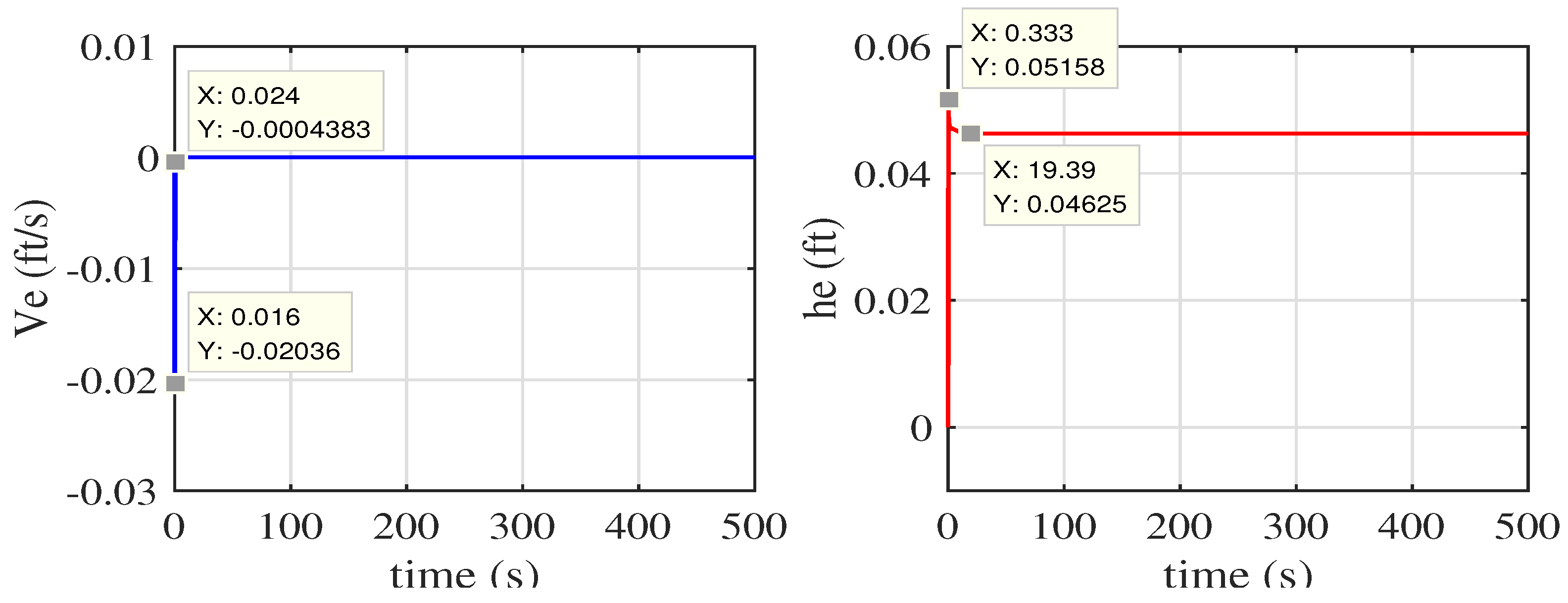
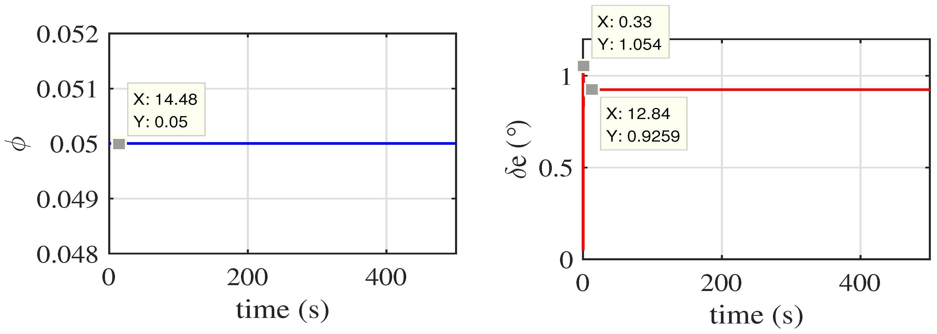
Set the target velocity and altitude as 8000 ft/s and 80,000 ft respectively, and use PID controller to certify the accuracy and controlability of the model. Parameters of controller is set as $K_{\varphi }=[20,0.1,0]$ and $K_{{\delta }_e}=[20,0,0.1]$. As shown in Figure 3 and Figure 4, the model can achieve horizontal flight under the control of PID controller. The longitudinal velocity error is almost 0 and the altitude error becomes stable at $0.05ft$. As control value, the fuel equivalent is stable at its minimum value. In the horizontal flight mode, fuel equivalent is ineffective and elevator deviation has a small deflection to balance gravity.

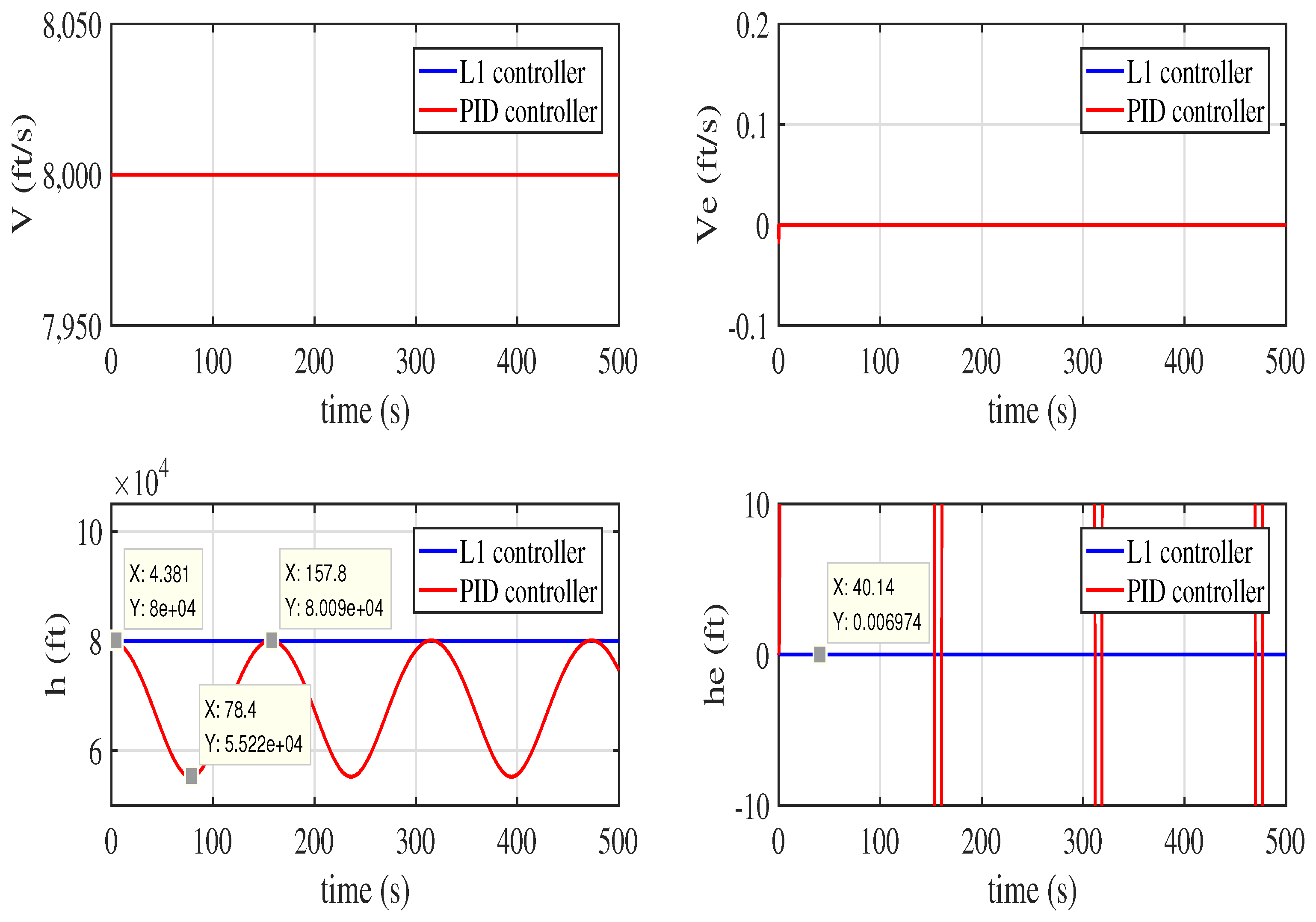
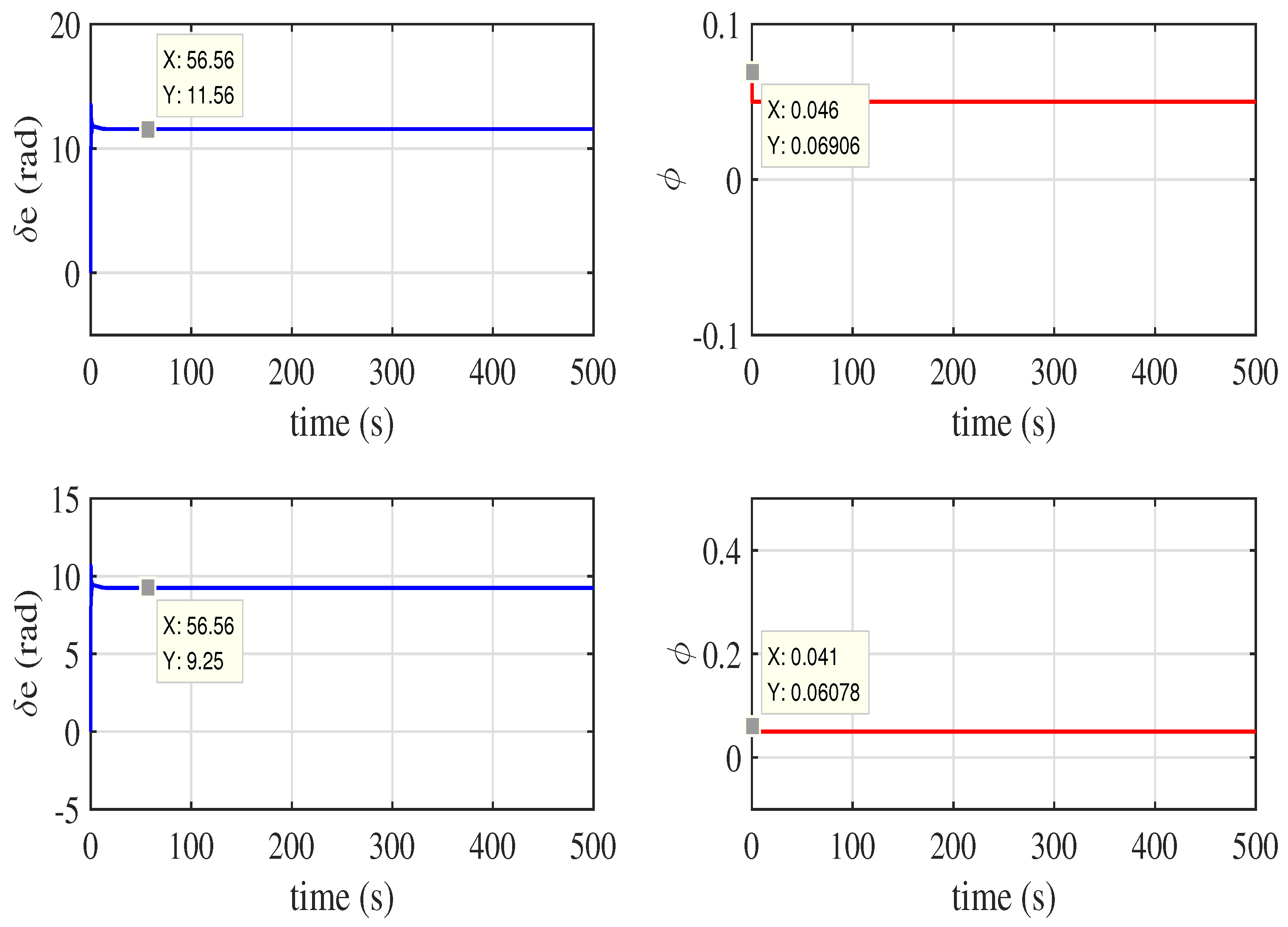
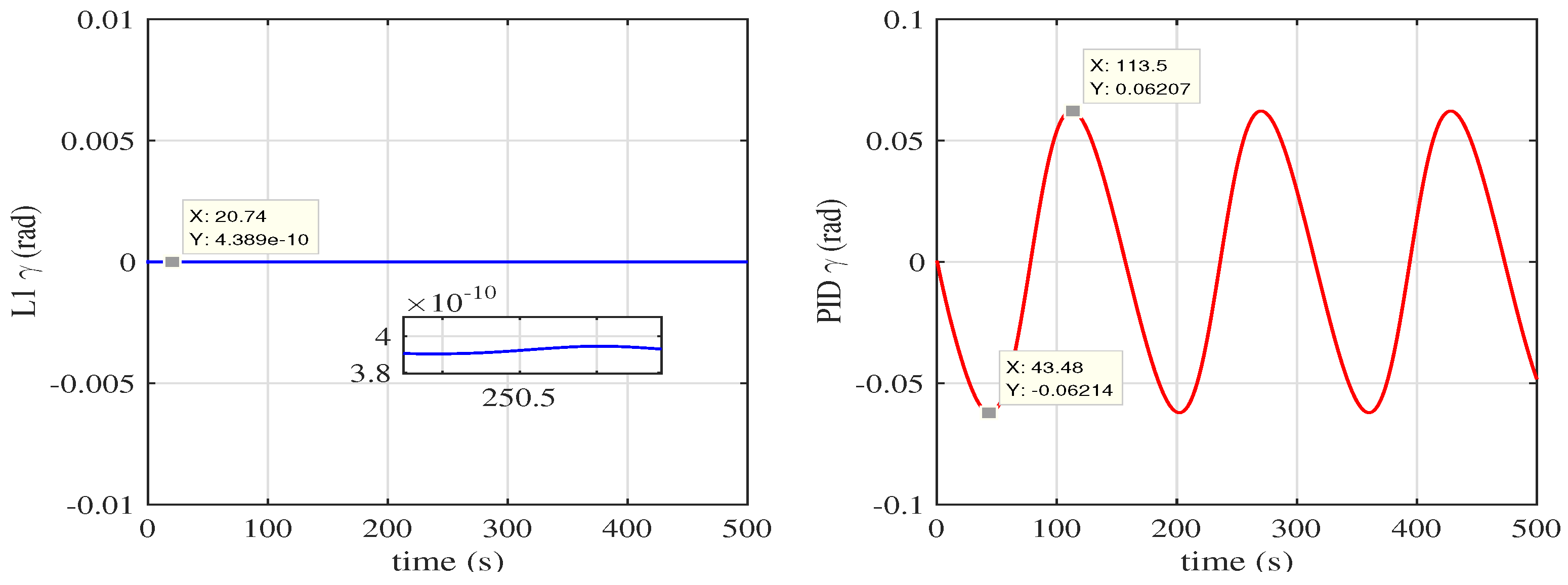
From 0 to 1, the loss fault rate increases by 0.05 each time. After a sequence of test, in the state of horizontal flight, the maximum fault rate the PID controller can tolerate is 0.35. Between 0.35–0.5, longitudinal velocity can be controlled but the altitude is unwarrantable. If the actuator loss exceeds 0.5, the whole system will be out of contol. Figure 5, Figure 6 and Figure 7 are the comparison of PID controller and ${\mathcal{L}}_1$ adaptive fault tolerance controller at fault rate 0.45. It is obvious that ${\mathcal{L}}_1$ adaptive fault tolerance controller is more advanced than PID controller in horizontal flight. Both controllers have almost the same performance at longitudinal velocity control. But both curves of altitude and track angle oscillate obviously with PID controller. By contrast, the ${\mathcal{L}}_1$ adaptive fault tolerance controller makes both the altitude error and track angle almost stable at 0.

4.2. Pitching Maneuver

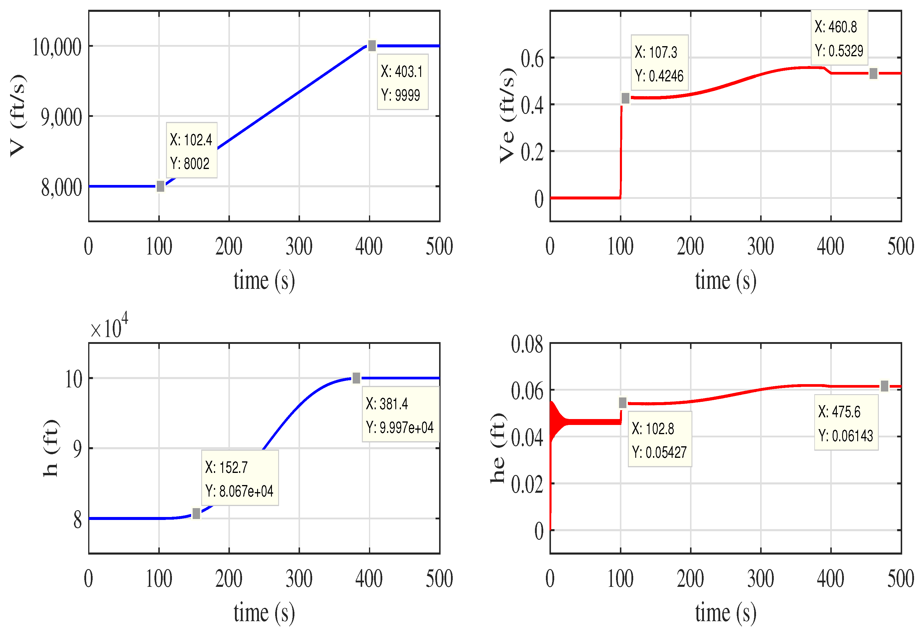
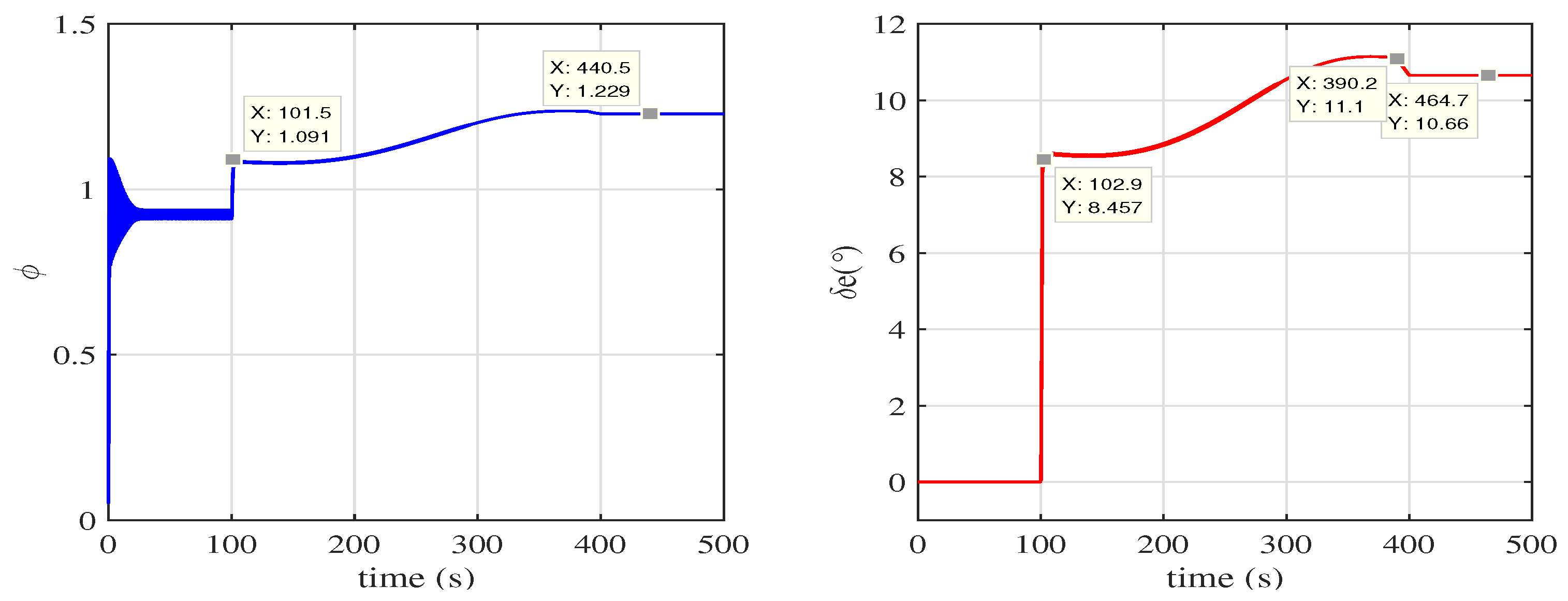
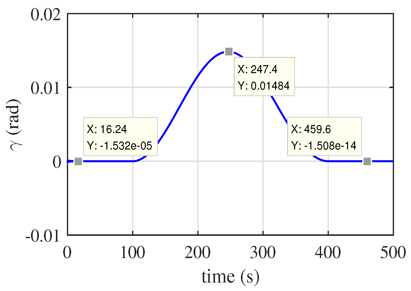
Pitching maneuver is a very important maneuver of hypersonic vehicle and it is more difficult to control. Actuator loss fault may lead to terrible results especially on upward flight. This paper uses the trajectory shown in [8] whichs has proved that aerodynamic hazards will not occur in this flight trajectory. Longitudinal velocity function and altitude function are shown in Equations (55) and (56). $V_{final}=$ 10,000 ft/s and $h_{final}=$ 100,000 ft. PID controller is used to make sure the model has the ability to achieve pitching maneuver. Control parameters is set as $K_{\varphi }=[20,0,0]$ and $K_{{\delta }_e}=[20,0,0]$. As shown in Figure 8, Figure 9 and Figure 10, the model can make pitching maneuver. PID controller can make the longitudinal error in 0.6 ft/s and altitude error in 0.06 ft with no fault. As shown in Figure 9, fuel equivalent contributes a lot in pitching maneuver. The track angle changes around 0.015 rad and finally returns to 0.

$$V_{\mathrm{r}}=\left\{\begin{array}{ccc}{V}_0& ,& 0\le t\le 100\\ V_0+10{(t-100)}^2/29& ,& 100\le t\le 110\\ V_0+200(t-105)/29& ,& 110\le t\le 390,\\ V_0+2000-10{(t-400)}^2/29& ,& 390\le t\le 400\\ V_{final}& ,& t\ge 400\end{array}\right.$$

(55)

$$h_r=\left\{\begin{array}{ccc}{h}_0& ,& 0\le t\le 100\\ \begin{array}{c}-{10}^{5}cos[2\pi (t-100)/300\hfill \\ -\pi /2]+h_0+(t-100)/300\hfill \end{array}& ,& 100\le t\le 400.\\ h_{final}& ,& t\ge 400\end{array}\right.$$

(56)

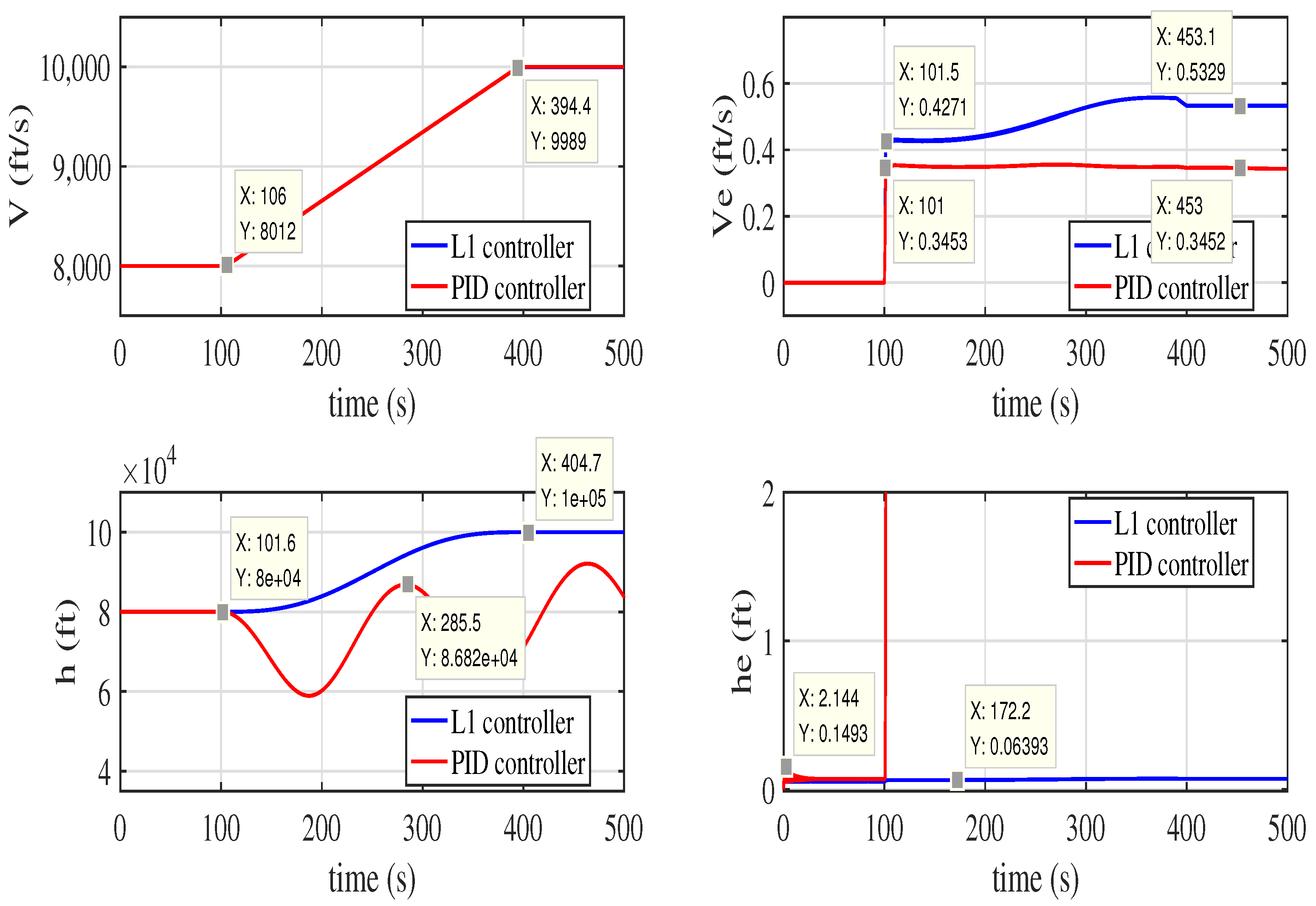
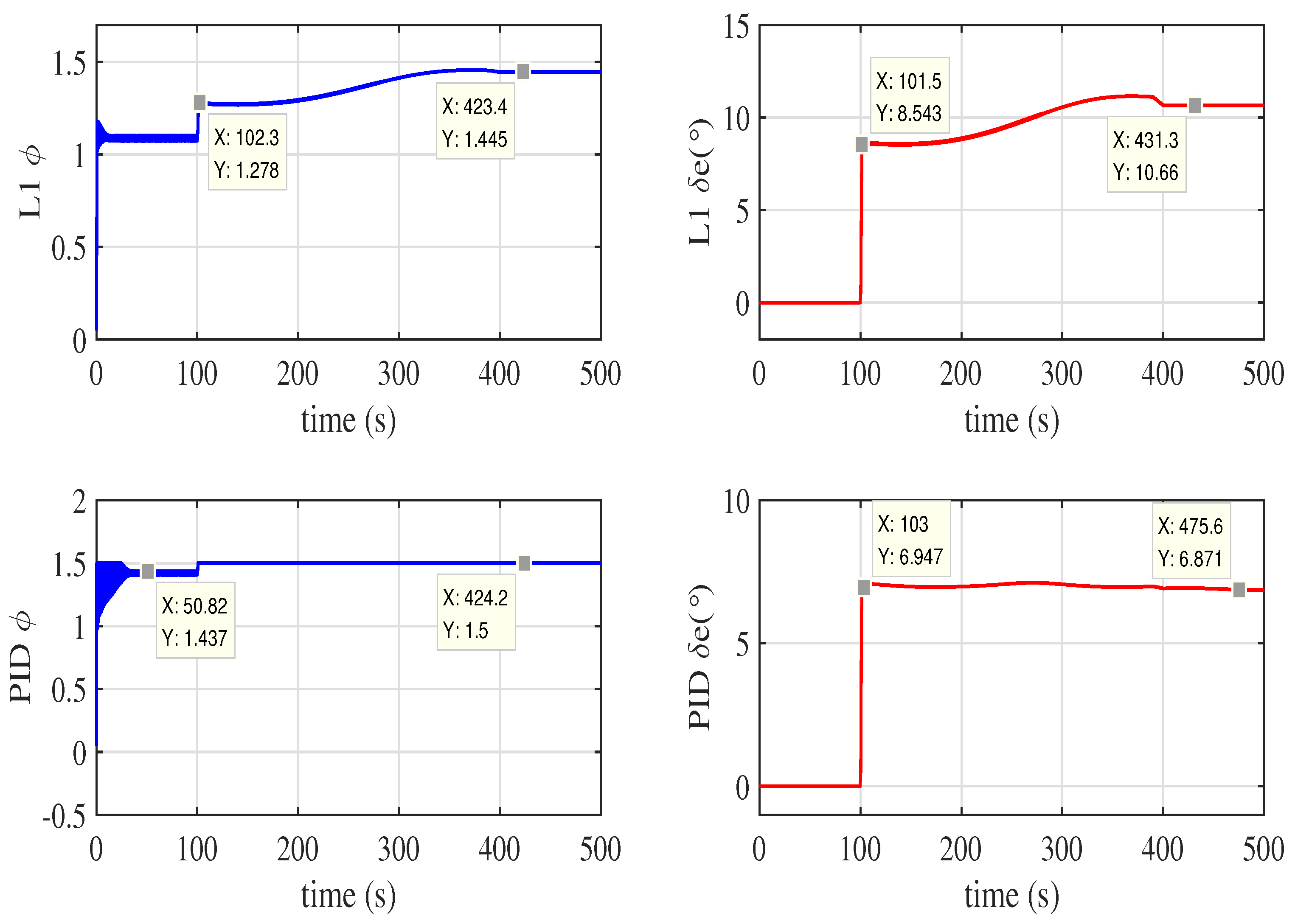
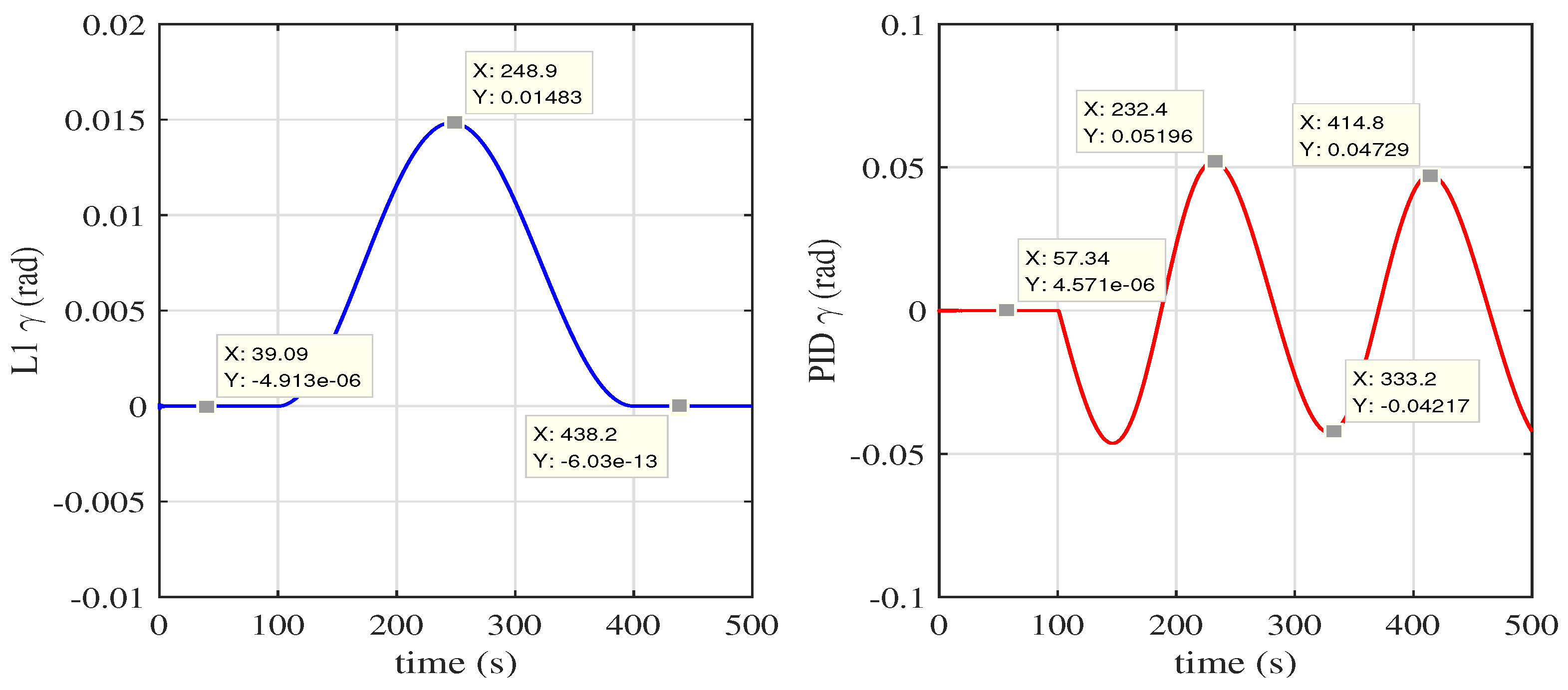
As the test in horizontal flight, it is figured out in pitching maneuver flight that the maximum fault rate PID controller can tolerate is 0.15 which is apparently smaller in horizontal flight. Between 0.15–0.35, velocity can be controlled while altitude cannot. Velocity and altitude will be out of control if the rate exceeds 0.4. The results at fault rate of 0.35 are shown in Figure 11, Figure 12 and Figure 13. Although PID controller has advantages in velocity control, the altitude is completely out of control. PID has better performance in longitudinal velocity control and can make the velocity error in 0.4 ft/s. Although ${\mathcal{L}}_1$ adaptive fault tolerance controller makes the velocity error in 0.6 ft/s, the altitude error is almost 0. Taken together, ${\mathcal{L}}_1$ adaptive fault tolerance controller is better.

In summary, Figure 3 and Figure 4 are the results by using PID controller in horizontal flight with no fault and it can make hypersonic vehicle stable. Figure 5, Figure 6 and Figure 7 are the comparison of PID controller and ${\mathcal{L}}_1$ controller in horizontal flight with 0.45 loss fault. It can be seen that ${\mathcal{L}}_1$ controller has better performance especially in altitude control. Figure 8, Figure 9 and Figure 10 are the results by using PID controller in pitching maneuver with no fault and the hypersonic vehicle can achieve pitching maneuver with no fault. Figure 11, Figure 12 and Figure 13 are the comparison of PID controller and ${\mathcal{L}}_1$ controller in horizontal flight with 0.35 loss fault. PID controller is better at velocity control but considering the velocity control and altitude control ${\mathcal{L}}_1$ controller has advantages in fault tolerance state.

5. Conclusions

This paper has presented ${\mathcal{L}}_1$ adaptive controllers for hypersonic aircraft to achieve loss fault tolerance control. The nonlinear and coupling mathematical model with elasticity of the hypersonic aircraft is built with the consideration of uncertainties. This paper investigates the combination of ${\mathcal{L}}_1$ adaptive control method and fault tolerance concept applying in hypersonic aircrafts. According to different aircrafts situations, this paper proposed two combination methods of ${\mathcal{L}}_1$ adaptive control and fault tolerance control. One is based on the fault tolerance ability of ${\mathcal{L}}_1$ adaptive controller, the other is adding compensators in cotroller design progress. The fault tolerance control method is applied in hypersonic aircraft, ${\mathcal{L}}_1$ adaptive controllers of velocity and altitude are designed respectively. Compared with the results of PID controller in loss fault state, the ${\mathcal{L}}_1$ adaptive controller can make sure that the hypersonic aircraft flight in an expected velocity and altitude at higher loss fault rate. Besides, it has better performance and less error than PID controller. ${\mathcal{L}}_1$ adaptive controller is advantageous in fault tolerance control of hypersonic aircrafts. There are still some things to do to enrich this paper. In the future work, we can add some other kinds of faults such as stuck, drifting and saturated to prove the fault tolerance ability of ${\mathcal{L}}_1$ fault tolerance adaptive controller and also there are many other advanced control methods or strategies with superior performances can be taken into consideration.

References

- Lewis, M. X-51 Screams into the Future. Aerosapce Am. 2010, 4, 26–31. [Google Scholar]
- Laurent, S.; Francois, F. Promethee—The French Military Hypersonic Propulsion Program. In Proceedings of the 12th AIAA International Space Planes and Hypersonic Systems and Technologies, Norfolk, VA, USA, 28–30 July 2012. [Google Scholar]
- Park, C. Hypersonic Aerothermodynamics: Past, Present and Future. Int. J. Aeronaut. Space Sci. 2013, 14, 1–10. [Google Scholar] [CrossRef] [Green Version]
- Wei, H.; Zhao-bo, D.; Li, Y. Supersonic mixing in airbreathing propulsion systems for hypersonic flights. Prog. Aerosp. Sci. 2019, 109. [Google Scholar]
- Hambling, D. China, Russia and the US in hypersonic arms race. New Sci. 2019, 243, 12. [Google Scholar] [CrossRef]
- Parker, J.T.; Serrani, A.; Yurkovich, S.; Bolender, M.A.; Doman, D.B. Control-oriented modeling of an air-breathing hypersonic vehicle. J. Guid. Control Dyn. 2007, 30, 856–869. [Google Scholar] [CrossRef]
- Fiorentini, L. Nonlinear Adaptive Controller Design for Air-Breathing Hypersonic Vehicles; The Ohio State University: Columbus, OH, USA, 2010. [Google Scholar]
- Linqi, Y.; Qun, Z.; Xiuyun, Z. Adaptive Control for a Non-minimum Phase Hypersonic Vehicle Model. In Proceedings of the 34th Chinese Control Conference, Hangzhou, China, 28–30 July 2015. [Google Scholar]
- Liu, Y.; Tong, Y.; Jin, F. Control law design of hypersonic vehicles using the elastic surrogate model. J. Low Freq. Noise Vib. Act. Control 2020, 39, 216–229. [Google Scholar] [CrossRef] [Green Version]
- Zhou, D.; Lu, Z.; Guo, T.; Shen, E.; Wu, J.; Chen, G. Fluid-thermal modeling of hypersonic vehicles via a gas-kinetic BGK scheme-based integrated algorithm. Aerosp. Sci. Technol. 2020, 99. [Google Scholar] [CrossRef]
- Li, Z.; Zhou, W.; Liu, H. Robust Controller Design of Non-minimum Phase Hypersonic Aircrafts Model based on Quantitative Feedback Theory. J. Astronaut. Sci. 2020, 67, 137–163. [Google Scholar] [CrossRef]
- Jia, J.; Fu, D.; He, Z.; Yang, J.; Hu, L. Hypersonic aerodynamic interference investigation for a two-stage-to-orbit model. ACTA Astronaut. 2020, 168, 138–145. [Google Scholar] [CrossRef]
- An, H.; Guo, Z.; Wang, G.; Wang, C. Low-complexity hypersonic flight control with asymmetric angle of attack constraint. Nonlinear Dyn. 2020. [Google Scholar] [CrossRef]
- Cheng, Z.; Chen, F.; Gong, J. Self-repairing control of air-breathing hypersonic vehicle with actuator fault and backlash. Aerosapce Sci. Technol. 2020, 97. [Google Scholar] [CrossRef]
- Sun, J.G.; Li, C.M.; Guo, Y.; Wang, C.Q.; Li, P. Adaptive fault tolerant control for hypersonic vehicle with input saturation and state constraints. ACTA Astronaut. 2020, 167, 302–313. [Google Scholar] [CrossRef]
- Tang, X.; Zhai, D.; Li, X. Adaptive fault-tolerance control based finite-time backstepping for hypersonic flight vehicle with full state constrains. Inf. Sci. 2020, 507, 53–66. [Google Scholar] [CrossRef]
- Dong, C.; Liu, Y.; Wang, Q. Barrier Lyapunov function based adaptive finite-time control for hypersonic flight vehicles with state constraints. ISA Trans. 2020, 9, 163–176. [Google Scholar] [CrossRef]
- Wang, A.; Gong, H.; Chen, F. Fault estimation and compensation for hypersonic flight vehicle via type-2 fuzzy technique and cuckoo search algorithm. Int. J. Adv. Robot. Syst. 2020, 17. [Google Scholar] [CrossRef] [Green Version]
- Thu, K.M.; Gavrilov, A.I. Designing and modeling of quadcopter control system using L1 adaptive control. Int. Symp. Intell. Syst. 2017, 103, 528–535. [Google Scholar]
- Zuo, Z.; Ru, P. Augmented L1 adaptive tracking control of quad-rotor unmanned aircrafts. IEEE Trans. Aerosp. Electron. Syst. 2014, 5, 3090–3101. [Google Scholar] [CrossRef]
- Xu, D.; Whidborne, J.; Cooke, A. Fault tolerant control of a quadrotor using L1 adaptive control. Int. J. Intell. Unmaaned Syst. 2016, 4, 43–66. [Google Scholar] [CrossRef] [Green Version]
- Li, M.; Zuo, Z.; Liu, H. Adaptive fault tolerant control for trajectory tracking of a quadrotor helicopter. Trans. Inst. Meas. Control 2018, 40, 3560–3569. [Google Scholar] [CrossRef]
- Cao, C.; Hovakimyan, N. L1 adaptive control theory. Soc. Ind. Appl. Math. 2010. [Google Scholar] [CrossRef]
- Sigthorsson, D.O.; Jankovsky, P.; Serrani, A.; Yurkovich, S.; Bolender, M.A.; Doman, D.B. Robust linear output feedback control of an airbreathing hypersonic vehicle. J. Guid. Control Dyn. 2008, 31, 1052–1066. [Google Scholar] [CrossRef]
Figure 1.
adaptive controller.
Figure 2.
Fault tolerance of hypersonic aircraft by adaptive control.
Figure 3.
Velocity error and altitude error proposed by PID controller in horizontal flight and fault free state.
Figure 4.
Control value proposed by PID controller in horizontal flight and fault free state.
Figure 5.
Comparison of velocity and velocity error, altitude and altitude error proposed by PID and controller in horizontal flight and fault state.
Figure 6.
Comparison of control value proposed by PID and controller in horizontal flight and fault state.
Figure 7.
Track angle proposed by PID and controller in horizontal flight and fault state.
Figure 8.
Velocity error and altitude error proposed by PID controller in pitching maneuver and fault free state.
Figure 9.
Control value proposed by PID controller in pitching maneuver and fault free state.
Figure 10.
Track angle proposed by PID controller in pitching maneuver and fault free state.
Figure 11.
Comparison of velocity and velocity error, altitude and altitude error proposed by PID and controller in pitching maneuver and fault state.
Figure 12.
Comparison of control value proposed by PID and controller in pitching maneuver and fault state.
Figure 13.
Comparison of track angle proposed by PID and controller in pitching maneuver and fault state.