Stereo Vision-Based Relative Position and Attitude Estimation of Non-Cooperative Spacecraft

Abstract

In on-orbit services, the relative position and attitude estimation of non-cooperative spacecraft has become the key issues to be solved in many space missions. Because of the lack of prior knowledge about manual marks and the inability to communicate between non-cooperative space targets, the relative position and attitude estimation system poses great challenges in terms of accuracy, intelligence, and power consumptions. To address these issues, this study uses a stereo camera to extract the feature points of a non-cooperative spacecraft. Then, the 3D position of the feature points is calculated according to the camera model to estimate the relationship. The optical flow method is also used to obtain the geometric constraint information between frames. In addition, an extended Kalman filter is used to update the measurement results and obtain more accurate pose optimization results. Moreover, we present a closed-loop simulation system, in which the Unity simulation engine is employed to simulate the relative motion of the spacecraft and binocular vision images, and a JetsonTX2 supercomputer is involved to conduct the proposed autonomous relative navigation algorithm. The simulation results show that our approach can estimate the non-cooperative target’s relative pose accurately.

1. Introduction

Nowadays, the space application capacity of various countries has been continuously improved. At the same time, space wastes, such as faulty spacecraft, retired spacecraft, and space debris, are increasing significantly. Cleaning up, repairing, and refueling techniques have also become increasingly important in on-orbit services [1,2]. To complete these services, two kinds of spacecraft exist, namely, chaser spacecraft and target spacecraft. The active side of on-orbit services is the chaser spacecraft, whereas the passive side is the target spacecraft. The target spacecraft must be captured and should perform appropriate operations in orbit. Autonomous relative navigation, which is one of the key technologies to complete the on-orbit services, can provide relative position and attitude for the acquisition, supporting the subsequent operations such as approaching, docking, and capture [3,4].

At present, most kinds of spacecraft in orbit are non-cooperative targets (NCTs). Due to the lack of prior knowledge about manual marks and the inability to communicate between two kinds of spacecraft, tracking and identifying the target are difficult to perform. The relative navigation of NCTs is difficult but critical, and has gradually obtained great attention [5,6,7]. In space missions aspects, the United States proposed the famous “Orbital Express” project based on a laser rangefinder and optical imaging sensor to complete the rendezvous and docking relative navigation in the process [7]. Compared with lidar, the optical navigation method has lower power consumption and higher accuracy, which makes it an important part of the autonomous navigation system and is widely used in the navigation of deep space exploration. Sweden successively launched two satellites called “PRISMA,” as the chaser spacecraft and the target spacecraft. In this project, the chaser spacecraft treats the target spacecraft as an NCT to conduct rendezvous and docking operations. The chaser spacecraft only relies on an optical camera to complete the navigation task, which proves the feasibility of the optical camera as a measurement sensor [8]. In academic research aspects, numerous research institutions and scholars have carried out independent research on the relative navigation technology of NCTs from the aspects of the construction of navigation schemes, the development of single sensor, the design of related algorithms, and so on. American engineers Woods and Christian used the 3D point cloud of a non-cooperative spacecraft through lidar to calculate the relative pose and complete the navigation task [9]. Qiu et al. [10] calculated the relative measurement of a non-cooperative spacecraft by using a visible light angle measuring camera and a laser rangefinder simultaneously. They also designed filters for the two sensors. In addition, the federated filter for data fusion was designed to obtain the final measurement. Aghili et al. [11] presented a robust six-degree-of-freedom relative navigation system by combing the iterative closet point (ICP) registration algorithm and a noise adaptive with measurements from a laser scanner and an inertial measurement unit (IMU). Augenstein et al. [12] presented a hybrid algorithm for real-time frame-to-frame pose estimation during monocular vision-only SLAM/SFM. Ruel et al. [13] presented results from the first two Space Shuttle test flights of the TriDAR vision system. Relative navigation of NCTs usually involves coordinate extraction process, especially for targets such as those with fast spinning, abnormal maneuvering, small size and lack of surface information. Lichter [14] developed a method for simultaneously estimating dynamic state, model parameters, and geometric shape of arbitrary space targets, using information gathered from range imaging sensors. Setterfield et al. [15] addressed the mapping and determining the center of mass of a rotating object task by using an observer that measures its orientation, angular rate and acceleration. Tweddle et al. [16] presented an experimental evaluation of on-board, visual mapping of an object spinning in micro-gravity aboard the international space station. Lyzhoft et al. [17] proposed a new image processing algorithm for terminal guidance of multiple kinetic-energy impactors for disrupting hazardous asteroids. Baichun et al. [18] developed a closed-form solution to the angles-only initial relative orbit determination problem for non-cooperative target close-in proximity operations when the camera offset from the vehicle center-of-mass allows for range observability.

Scholars have also conducted research on NCTs motion estimation by using stereo vision sensors and extended Kalman filters (EKF). Zhou et al. [19] proposed a method to calculate the relative state based on stereo vision by using the chaser spacecraft moment model and slave spacecraft gyro. In the absence of chaser spacecraft dynamic information, the Clohessy–Wiltshire equation and state equation can be used to complete the joint filtering, which can estimate the relative state well. Segal et al. [20] extracted the feature points of a target spacecraft, calculated the relative posture as the state quantity by using the observation model of a binocular camera, and finally optimized the relative measurement using the iterative EKF method. Pesce et al. [21] established an attitude-orbit coupling motion model of feature points on the surface and estimated attitude and principal axis inertia ratio by observing the feature points with a stereo camera. Feng et al. [22] also extracted feature points from binocular camera images and estimated the relative posture by using the least square method. The convex optimization method was used to estimate the inertial parameters of the spacecraft. Son-Goo K et al. [23] obtained the relative posture and the deviation of the gyroscope by combining the measurement information from multiple sensors and the dynamic model. In addition, the measurements of the visual system were used as observation information to update the extended Kalman filter (EKF). Yoko [24] estimated the position and velocity of a target by using the measurement information obtained from a monocular camera. The final pose estimation result was obtained using the EKF [25] algorithm. Compared with monocular cameras, binocular stereo vision cameras can provide a wider field of view and can perform 3D reconstruction.

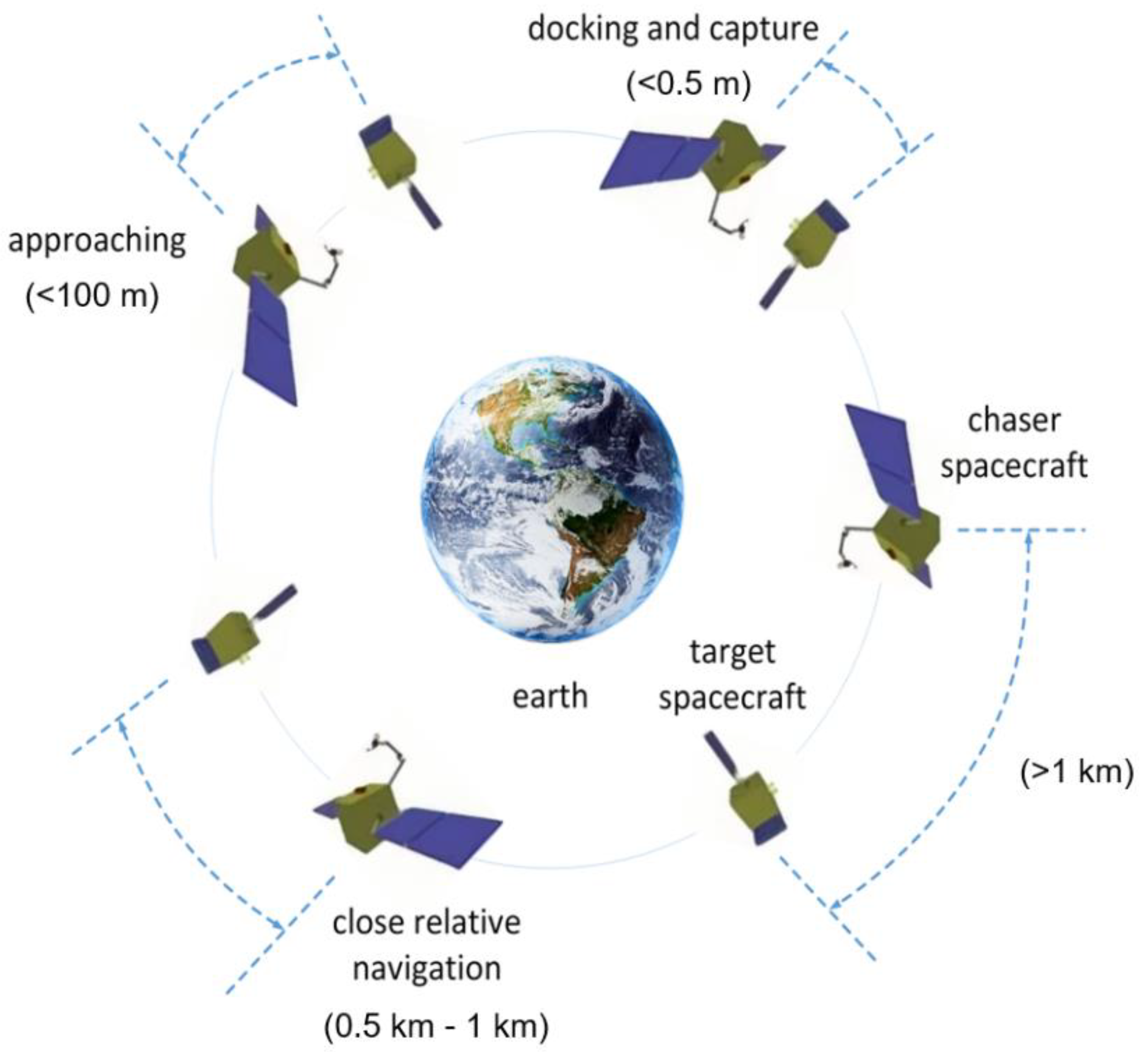
The process of orbit service missions for non-cooperative spacecraft can be divided into four stages: long-range guidance, short-range guidance, the approaching phase, docking and capture [6], as shown in Figure 1. In the approaching phase, the distance between the two kinds of spacecraft is approximately 100 m. In this phase, sensors such as optics must be used to accurately measure the relative position, relative speed, relative angular velocity, and relative attitude angle of the target spacecraft. Hence, the chaser spacecraft can complete the maneuver automatically, meeting the requirements of the docking and capture phase [2].

Based on the parallax measurement principle, the effective measurement depth of binocular vision is usually within 20 m. Most traditional binocular stereo vision-based relative navigation systems need to recognize the artificial marks mounted on the target spacecraft. However, these elaborated, artificial marks cannot be preset on a non-cooperative spacecraft. The autonomous relative navigation algorithm needs to extract the feature points that can be used for stereo measurement, automatically and intelligently. This work mainly concerns the stereo measurement modeling, data management and calculation technology for NCT relative navigation in the phase of approaching and closer range. We derive the system state equation of the EKF algorithm using the relative orbit dynamics model and the relative attitude dynamics model to predict the prior state, i.e., the relative position, relative velocity, relative angular velocity and relative attitude angle of the target spacecraft. Additionally, then, the prior state is updated by using the binocular observation information. Higher accuracy can be obtained after sequentially filtering. We further verify the relevant algorithm through a closed-loop simulation and experiment.

This paper intends to provide some technical details for autonomous relative navigation in future on-orbit rescue missions. The present work has three potential contributions: (1) to propose an optical flow method to track and match the feature points of the images, to solve the challenge of disastrous mismatching of feature points caused by serious repeated textures on the surface of NCTs under complex lighting conditions; (2) to introduce in detail a feature point management method which can balance the calculation efficiency and matching accuracy; and (3) to present a JetsonTX2 supercomputer-involved closed-loop simulation system, in which the dynamic-based relative navigation filtering algorithm is designed, simulated and tested.

The structure of this paper is as follows: in Section 2, we introduce the proposed relative pose measurement of the NCT method. In Section 3, the implementation details of the closed-loop simulation system are presented. In Section 4, we analyze and discuss the simulation results of the relative pose measurement of the NCT. In Section 5, we conclude our work.

2. Materials and Methods

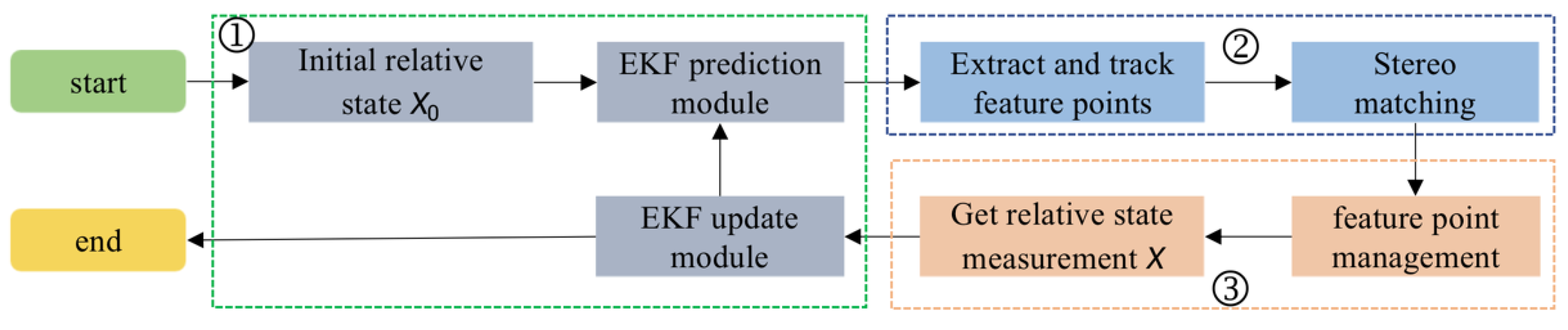
This study mainly investigates the autonomous relative navigation technology of a space NCT in the final approaching stage. We propose a precise measurement of the relative posture algorithm based on binocular vision and dynamic model error analysis. This method can accurately measure the relative position, relative velocity, relative angular velocity and relative attitude of the target spacecraft. The overall algorithm design scheme is illustrated in Figure 2.

The state dynamic equation is regarded as the filter motion equation. First, the predicted pose results are obtained by the EKF prediction module, using the relative orbit dynamics and the relative attitude dynamics model. Then, the target feature points in the binocular camera image are extracted by using the Features from Accelerated Segment Test (FAST) algorithm, and the 3D position of the points is calculated according to the convergent binocular stereo vision measurement. More representative feature points can be acquired and tracked between frames by using the optical flow method. A stereo-matching approach is used to obtain the geometric constraint information between the frames. The relative attitude and angular velocity are first calculated from the tracked feature points, and then position and velocity. Finally, the measurement results are optimized through the EKF update module to obtain final results with less error.

2.1. Status Model

The state vector of the target spacecraft can be defined as

$$X={\left[\begin{array}{ccc}{q}_{ct}^T& {\omega }_{tc}^t{}^T& x_p^T\end{array}\right]}^T$$

(1)

where $q_{ct}$ is a quaternion and denotes relative attitude, ${\omega }_{tc}^t$ denotes relative angular velocity, and $x_p^T$ denotes relative position and relative velocity. One can refer to the state equation of the relative motion of spacecraft:

$${\dot{\widehat{q}}}_{ct}=\frac{1}{2}\left[\begin{array}{c}{\widehat{\omega }}_{tc}^t\\ 0\end{array}\right]\otimes {\widehat{q}}_{ct}$$

(2)

$${\dot{\omega }}_{tc}^t=I_t^{-1}\left(T^t-\left[\left({\omega }_{tc}^t+R_c^t{\omega }_{ci}^c\right)\times \right]\left(I_t\left({\omega }_{tc}^t+R_c^t{\omega }_{ci}^c\right)\right)\right)+{\omega }_{tc}^t\times {\omega }_{ci}^t-R_c^t{I}_c^{-1}\left(T^c-\left[{\omega }_{ci}^c\times \right]\left(I_c{\omega }_{ci}^c\right)\right)+I_t^{-1}{w}_a$$

(3)

$${\dot{\widehat{x}}}_p=F{\widehat{x}}_p$$

(4)

where $\otimes$ denotes the quaternion multiplication; $w_a$ denotes the white Gaussian noise;$T^c$ denotes the total moment of the chaser spacecraft; $T^t$ denotes the total moment of the target spacecraft; and $I_c$ and $I_t$ denote the inertia matrix of the chaser and target spacecraft, respectively.

The filter error state is defined as

$$\mathsf{\Delta }X={\left[\begin{array}{ccc}\delta a_{ct}^T& \mathsf{\Delta }{\omega }_{tc}^{tT}& \mathsf{\Delta }{x}_p^T\end{array}\right]}^T$$

(5)

where $\delta q_{ct}=q_{ct}\otimes {\widehat{q}}_{ct}^{-1}$, $\delta q_{ct}\approx \left[\begin{array}{c}\frac{1}{2}\delta a_{ct}\\ 1\end{array}\right]$, the relative angular velocity error is $\mathsf{\Delta }{\omega }_{tc}^t={\omega }_{tc}^t-{\widehat{\omega }}_{tc}^t$, and the error relative to the bit velocity is $\mathsf{\Delta }{x}_p=x_p-{\widehat{x}}_p$.

By definition of error, the following can be obtained:

$$q_{ct}=\delta q_{ct}\otimes {\widehat{q}}_{ct}$$

(6)

Combined with the attitude dynamics Equation (2), we have

$$\begin{gathered} \frac{1}{2}\left[\begin{array}{c}{\omega }_{tc}^t\\ 0\end{array}\right]\otimes q_{ct}=q_{ct}\otimes {\widehat{q}}_{ct}^{-1}+\frac{1}{2}\delta q_{ct}\otimes \left[\begin{array}{c}{\widehat{\omega }}_{tc}^t\\ 0\end{array}\right]\otimes {\widehat{q}}_{ct} \\ \delta {\dot{q}}_{ct}=\frac{1}{2}\left[\begin{array}{c}{\omega }_{tc}^t\\ 0\end{array}\right]\otimes \delta q_{ct}-\frac{1}{2}\delta q_{ct}\otimes \left[\begin{array}{c}{\widehat{\omega }}_{tc}^t\\ 0\end{array}\right] \end{gathered}$$

(7)

Substitute Equation (7) into ${\omega }_{tc}^t={\widehat{\omega }}_{tc}^t+\Delta {\omega }_{tc}^t$ and $\delta q_{ct}\approx \left[\begin{array}{c}\frac{1}{2}\delta a_{ct}\\ 1\end{array}\right]$, we can obtain

$$\delta {\dot{a}}_{ct}=-{\widehat{\omega }}_{tc}^t\times \delta a_{ct}+\mathsf{\Delta }{\omega }_{tc}^t$$

(8)

According to Equation (6), one can obtain

$$R\left(q_{ct}\right)=\left\{I_{3\times 3}-\left[\delta a_{ct}\times \right]\right\}R\left({\widehat{q}}_{ct}\right)$$

(9)

According to this equation, when the tracking spacecraft has and only has orbital angular velocity, it satisfies $R_c^t{I}_c^{-1}\left(T^c-\left[{\omega }_{ci}^c\times \right]\left(I_c{\omega }_{ci}^c\right)\right)=0$, then

$$\mathsf{\Delta }{\dot{\omega }}_{tc}^t=\frac{\partial {\dot{\omega }}_{tc}^t}{\partial \delta a_{ct}}\mathsf{\Delta }{a}_{ct}+\frac{\partial {\dot{\omega }}_{tc}^t}{\partial {\omega }_{tc}^t}\mathsf{\Delta }{\omega }_{tc}^t+I_t^{-1}{w}_a$$

(10)

According to ${\dot{x}}_p=F{x}_p+f$, we can obtain

$$\mathsf{\Delta }{\dot{x}}_p=F\mathsf{\Delta }{x}_p+\varpi$$

(11)

Thus, the dynamic equation of error state is:

$$\mathsf{\Delta }\dot{X}=F_{11}\mathsf{\Delta }X+Gw$$

(12)

where

$$F_{11}=\left[\begin{array}{ccc}-{\widehat{\omega }}_{tc}^t\times & I_{3\times 3}& 0_{3\times 6}\\ F_{\omega q}& F_{\omega \omega }& 0_{3\times 6}\\ 0_{6\times 3}& 0_{6\times 3}& F\end{array}\right]$$

(13)

$${\dot{\omega }}_{tc}^t=I_t^{-1}\left(T^t-\left[\left({\omega }_{tc}^t+R_c^t{\omega }_{ci}^c\right)\times \right]\left(I_t\left({\omega }_{tc}^t+R_c^t{\omega }_{ci}^c\right)\right)\right)+{\omega }_{tc}^t\times {\omega }_{ci}^t-R_c^t{I}_c^{-1}\left(T^c-\left[{\omega }_{ci}^c\times \right]\left(I_c{\omega }_{ci}^c\right)\right)+I_t^{-1}{w}_a$$

(14)

Since

$$u\times v=-v\times u$$

(15)

We further find:

$$\begin{gathered} \frac{\partial \left(\omega \times \left(I\omega \right)\right)}{\partial \omega }=\frac{\partial \left(\omega \times \left(I{\omega }_{\mathrm{static} }\right)\right)}{\partial \omega }+\frac{\partial \left({\omega }_{\mathrm{static} }\times \left(I\omega \right)\right)}{\partial \omega }=\frac{\partial \left(-\left(I{\omega }_{\mathrm{static} }\right)\times \omega \right)}{\partial \omega }+{\omega }_{\mathrm{static} }\times I \\ =-\left(I\omega \right)\times +\left(\omega \times \right)I \end{gathered}$$

(16)

$$\frac{\partial \left(Rp\right)}{\partial \phi }=-\left(Rp\right)\times$$

(17)

$$\begin{gathered} F_{\omega q}=\frac{\partial {\dot{\omega }}_{tc}^t}{\partial \delta a_{ct}}=\frac{\partial I_t^{-1}\left(T^t-\left[\left({\omega }_{tc}^t+R_c^t{\omega }_{ci}^c\right)\times \right]\left(I_t\left({\omega }_{tc}^t+R_c^t{\omega }_{ci}^c\right)\right)\right)}{\partial \delta a_{ct}}+\frac{\partial {\omega }_{tc}^t\times {\omega }_{ci}^t}{\partial \delta a_{ct}} \\ -\frac{\partial R_c^t{I}_c^{-1}\left(T^c-\left[{\omega }_{ci}^c\times \right]\left(I_c{\omega }_{ci}^c\right)\right)}{\partial \delta a_{ct}}+\frac{\partial I_t^{-1}{w}_a}{\partial \delta a_{ct}} \end{gathered}$$

(18)

When the target spacecraft does not maneuver, the total torque $T^t=0$. Let

$$F=\left({\omega }_{tc}^t+R_c^t{\omega }_{ci}^c\right)$$

(19)

Then, the following is easy to obtain:

$$\frac{\partial I_t^{-1}\left(T^t-\left[\left({\omega }_{tc}^t+R_c^t{\omega }_{ci}^c\right)\times \right]\left(I_t\left({\omega }_{tc}^t+R_c^t{\omega }_{ci}^c\right)\right)\right)}{\partial \delta a_{ct}}=-2\left[{\omega }_{tc}^{t}x\right]\left[\left(R_c^t{\omega }_{ci}^c\right)\times \right]$$

(20)

When the tracking spacecraft does not maneuver,

$$R_c^t{I}_c^{-1}\left(T^c-\left[{\omega }_{ci}^c\times \right]\left(I_c{\omega }_{ci}^c\right)\right)=0$$

(21)

and we have

$$\frac{\partial I_t^{-1}{w}_a}{\partial \delta a_{ct}}=0$$

(22)

Hence,

$$F_{\omega q}=2I_t^{-1}\left[-\left(I_t\left({\omega }_{tc}^t+R_c^t{\omega }_{ci}^c\right)\right)\times +\left({\omega }_{tc}^t+R_c^t{\omega }_{ci}^c\right)\times I_t\right]\cdot \left[\left(R_c^t{\omega }_{ci}^c\right)\times \right]-2\left[{\omega }_{tc}^t\times \right]\left[\left(R_c^t{\omega }_{ci}^c\right)\times \right]$$

(23)

$$F_{\omega \omega }=I_t^{-1}\left(-\left[\left({\omega }_{tc}^t+R_c^t{\omega }_{ci}^c\right)\times \right]I_t+\left[\left(I_t\left({\omega }_{tc}^t+R_c^t{\omega }_{ci}^c\right)\right)\times \right]\right)-\left(R_c^t{\omega }_{ci}^c\right)\times$$

(24)

$$G=\left[\begin{array}{cc}{0}_{3\times 3}& 0_{3\times 3}\\ I_t^{-1}& 0_{3\times 3}\\ 0_{3\times 3}& 0_{3\times 3}\\ 0_{3\times 3}& I_{3\times 3}\end{array}\right]$$

(25)

where $w={\left[\begin{array}{c}{\sigma }^T {\varpi }^T\end{array}\right]}^T$.

When the sampling time is short, the first-order approximate covariance matrix of discrete time is $\mathsf{\Delta }tGQ{G}^T$, and the state transition matrix is ${\mathsf{\Phi }}_{k+1,k}\approx I_{12\times 12}+F_{11}\mathsf{\Delta }t$.

2.2. Measurement Model

According to the binocular camera measurement model, the feature points in the image can be extracted and the 3D coordinates P of the feature points can be calculated. The position of the i-th feature point extracted under the camera system is ${\rho }_i={\left[\begin{array}{ccc}{\rho }_{ix}& {\rho }_{iy}& {\rho }_{iz}\end{array}\right]}^T$. The velocity of characteristic points is ${\dot{\rho }}_i={\left[\begin{array}{ccc}{\dot{\rho }}_{ix}& {\dot{\rho }}_{iy}& {\dot{\rho }}_{iz}\end{array}\right]}^T$, and the velocity of pixel points is

$$\left[\begin{array}{ccc}{f}_x& 0& c_x-{\overline{u}}_{iL}\\ 0& f_y& c_y-{\overline{v}}_{iL}\\ f_x& 0& c_x-{\overline{u}}_{iR}\\ 0& f_y& c_y-{\overline{v}}_{iR}\end{array}\right]\overline{{\dot{\rho }}_i}={\rho }_{iz}\left[\begin{array}{c}{\dot{\overline{u}}}_{iL}\\ {\dot{\overline{v}}}_{iL}\\ {\dot{\overline{u}}}_{iR}\\ {\dot{\overline{v}}}_{iR}\end{array}\right]$$

(26)

Therefore, the 3D velocity of feature points can be solved for subsequent calculation according to the pixel velocity of the optical flow method.

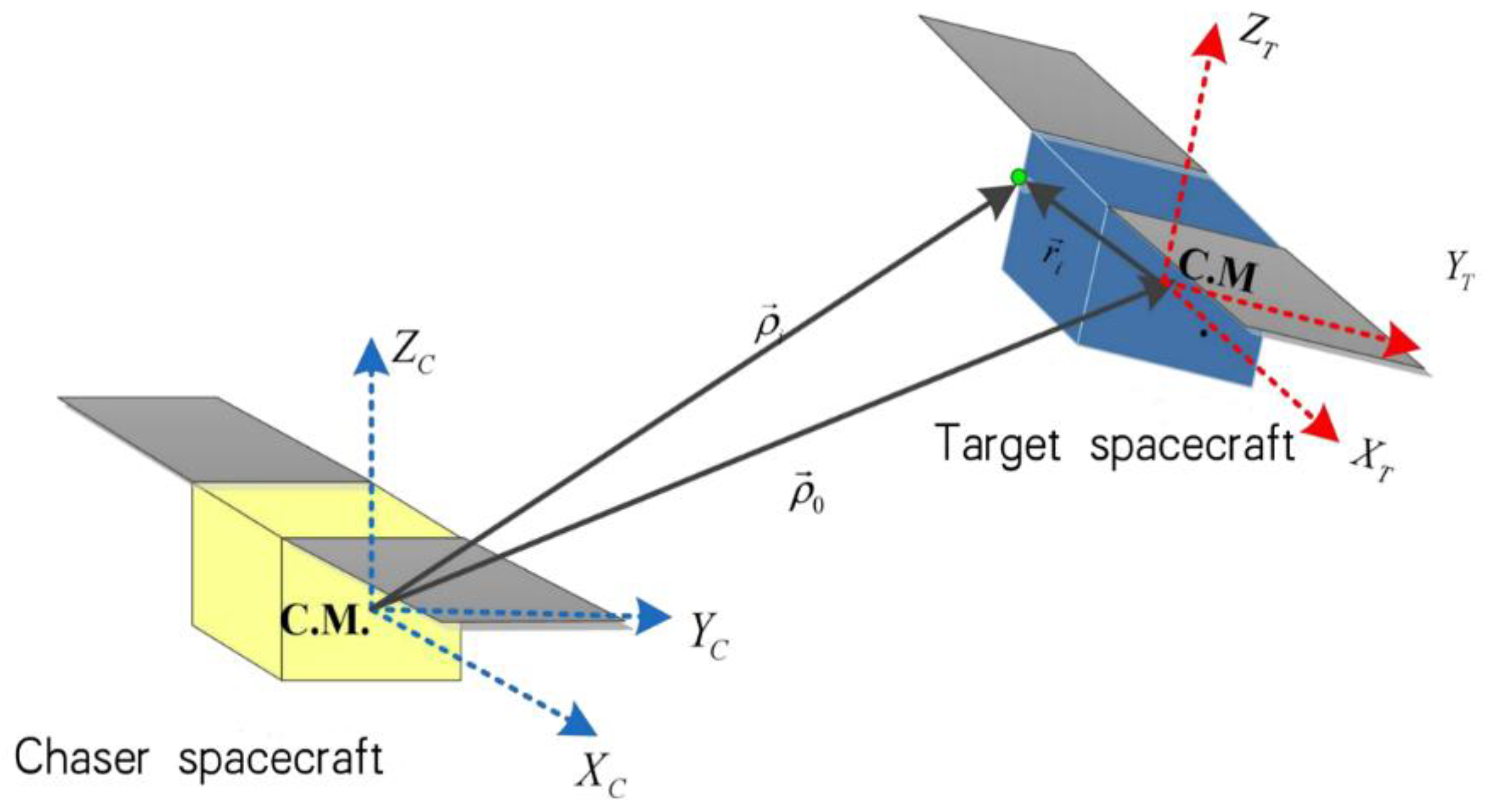
As displayed in Figure 3, the binocular camera can extract and calculate a set of 3D feature points ${\left\{P_i\right\}}_{i=1}^N$, where ${\stackrel{\rightharpoonup }{p}}_i$ is the vector from the origin of the tracking spacecraft coordinate system to ${\left\{P_i\right\}}_{i=1}^N$, ${\stackrel{\rightharpoonup }{p}}_0$ is the vector from the origin of the target spacecraft coordinate system to the center of mass of the target spacecraft, and ${\stackrel{\rightharpoonup }{r}}_i$ is the vector from the origin of the target spacecraft coordinate system to the feature point ${\left\{P_i\right\}}_{i=1}^N$ on the target spacecraft, that is, the position of the feature point in the target system.

According to Feng’s measurement model establishment method, the relative attitude, angular velocity, position, and velocity of the center of mass of the target spacecraft can be obtained [26].

First, we can use the 3D feature point set to obtain the relative attitude. The relative attitude can be solved according to the feature point association relationship between two consecutive frames. It mainly includes the following two steps: 1. select a reference point from the matching points and obtain two groups of three-dimensional vectors in two frames, namely the tracking spacecraft coordinate system and the target spacecraft coordinate system; 2. calculate the rotation matrix between the two coordinates, according to the vector observations. In essence, this is a Wahba’s problem [27]. There are many solutions to this problem, notably Davenport’s q-method, the Gauss Newton algorithm, QUEST and singular value decomposition-based methods. Among them, there is evidence that the q-method has the highest accuracy and stability [28], so the q-method is used in this paper. The intermediate process is omitted because it is cumbersome; only the final conclusion is given below. Define:

$$L\left(B\right)=\left[\begin{array}{cc}B+B^T-\left(trace\left(B\right)\right)I_{3\times 3}& z\\ z^T& trace\left(B\right)\end{array}\right]$$

(27)

where, $B={\sum }_{i=1}^N{\sigma }_i\delta {\rho }_i\left(t_k\right){\left(\delta {\rho }_i\left(t_0\right)\right)}^T$, $z={\sum }_{i=1}^N{\sigma }_i\left[\left[\delta {\rho }_i\left(t_k\right)\times \right]\delta {\rho }_i\left(t_0\right)\right]={\left[\begin{array}{c}{B}_{23}-B_{32}\hspace{1em}{B}_{31}-B_{13}\hspace{1em}{B}_{12}-B_{21}\end{array}\right]}^T$.

Optimized solution $\delta {\overline{q}}_{tc}\left(t_k\right)$ is the eigenvector $q_{opt}$, corresponding to the maximum eigenvalue ${\lambda }_{max}$ of L(B), namely:

$$L\left(B\right)q_{opt}={\lambda }_{max}{q}_{opt}$$

(28)

Second, by using the 3D feature point coordinates and the inter-frame difference velocity, the relative angular velocity can be calculated.

$${\overline{\omega }}_{tc}^c={\left({\left[\begin{array}{c}\delta {\rho }_1\times \\ ⋮\\ \delta {\rho }_{N-1}\times \end{array}\right]}^T\left[\begin{array}{c}\delta {\rho }_1\times \\ ⋮\\ \delta {\rho }_{N-1}\times \end{array}\right]\right)}^{-1}{\left[\begin{array}{c}\delta {\rho }_1\times \\ ⋮\\ \delta {\rho }_{N-1}\times \end{array}\right]}^T\left[\begin{array}{c}-\delta {\dot{\rho }}_1\\ ⋮\\ -\delta {\dot{\rho }}_{N-1}\end{array}\right]$$

(29)

Finally, the relative position and velocity can be calculated through substituting the relative attitude and angular velocity into the following equations.

$$\{\begin{array}{c}{\overline{\rho }}_0=\frac{1}{N}{\sum }_{i=1}^N\left[{\rho }_i-{\left[R_t^c{r}_i^t\right]}^{-}\right]\\ \overline{{\dot{\rho }}_0}=\frac{1}{N}{\sum }_{i=1}^N\left[{\dot{\rho }}_i-\left[{\overline{\omega }}_{tc}^c\times \right]{\left[R_t^c{r}_i^t\right]}^{-}\right]\end{array}$$

(30)

2.3. Feature Points Extraction, Tracking, and Matching

In this subsection, we describe in detail the process of feature points extraction, tracking, and matching. The famous FAST algorithm is used to extract the feature points from the binocular camera image [29]. According to the principle of binocular parallax measurement, we obtain the 3D coordinates of the feature points. The optical flow method is used to track and manage the feature points between the previous and subsequent frames. Finally, the relative posture, relative angular velocity, relative position and relative velocity measurement values are obtained from these continuous frame feature points.

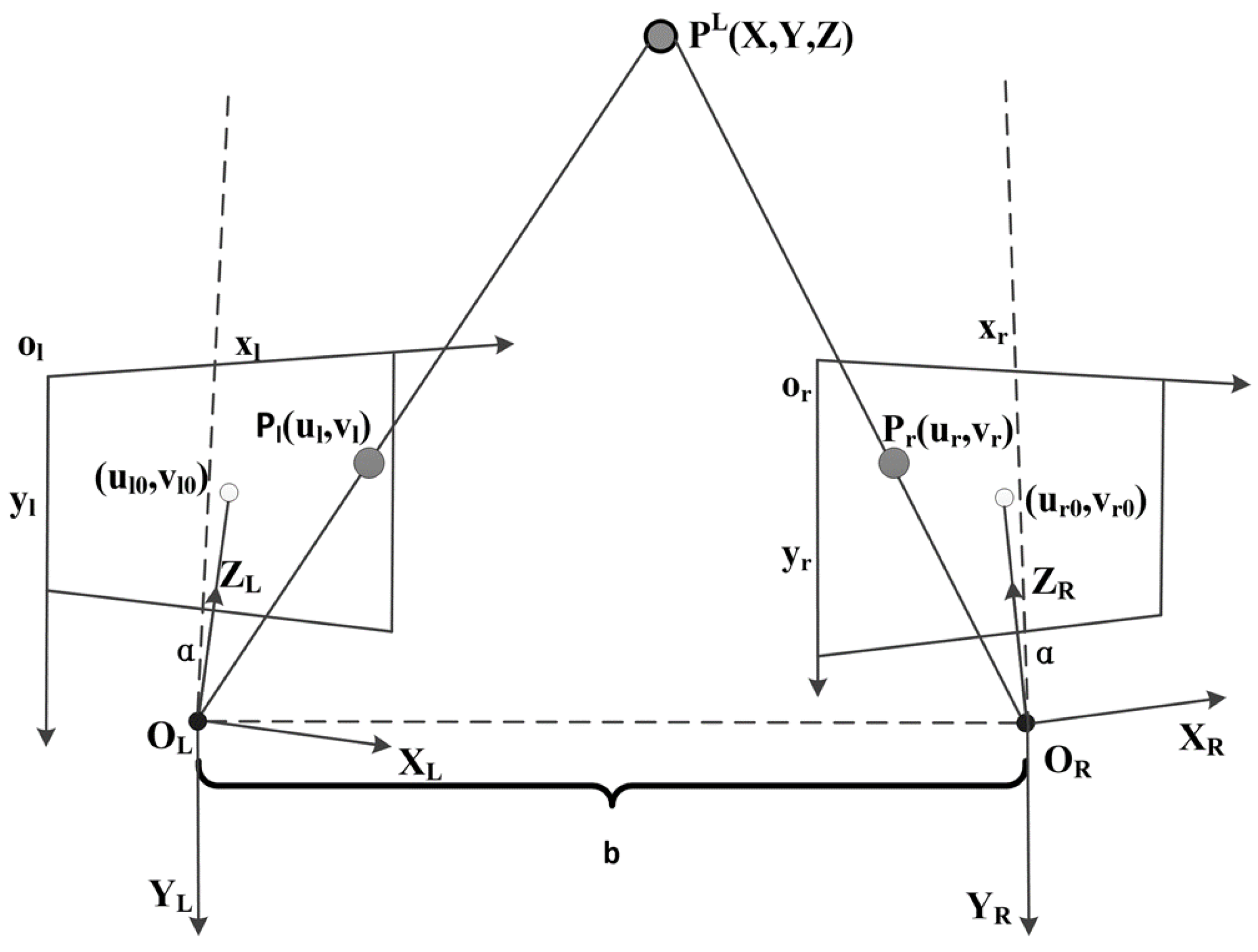
The measurement method based on the binocular camera for relative posture from the chaser spacecraft to the target spacecraft essentially uses the binocular camera on the chaser spacecraft to simultaneously obtain the image information of the target satellite from two different perspectives [30]. The posture of the target spacecraft in the camera coordinate system is then calculated by the binocular parallax principle. Then, it is converted to the coordinate system of the tracking spacecraft to obtain the 3D position information of these feature points. In our research, a convergent stereo vision system is used to provide the observation data. The principle of convergent binocular stereo vision measurement is shown in Figure 4.

The matched co-view feature point under the left camera coordinate system $P^L\left(X,Y,Z\right)$ can be marked as $\left(u_{l0},v_{l0}\right), \left(u_{r0},v_{r0}\right)$ on the left and right imaging planes, respectively. According to the triangle similarity principle, the point $P^L\left(X,Y,Z\right)$ can be obtained as:

$$\{\begin{array}{c}X=Z\frac{u_l-u_{l0}}{f}\\ Y=Z\frac{v_l-v_{l0}}{f}\\ Z=\frac{f·b\left(\tan \left(2\alpha +{\arctan }^{-1}\frac{u_{r0}-u_r}{f}-\frac{\pi }{2}\right)·\cos \alpha +\sin \alpha \right)}{\tan \left(2\alpha +{\arctan }^{-1}\frac{u_{r0-}{u}_r}{f}-\frac{\pi }{2}\right)·\left(u_l-u_{l0}\right)-f}\end{array}$$

(31)

To solve the challenge of not having artificial marks on NCTs, FAST feature points are extracted from the image captured by the binocular camera. If the difference between the value of a certain pixel and its surrounding pixels is greater than the threshold, and the number of pixels is greater than a certain threshold, then the pixel is determined as a feature point. The above steps may cause the problem of excessively concentrated feature point distribution. By calculating the response value of the feature point and sorting, the point with a small response value is removed. The response value is the sum of the absolute deviation of the corner pixel value and the surrounding 16 neighboring pixels.

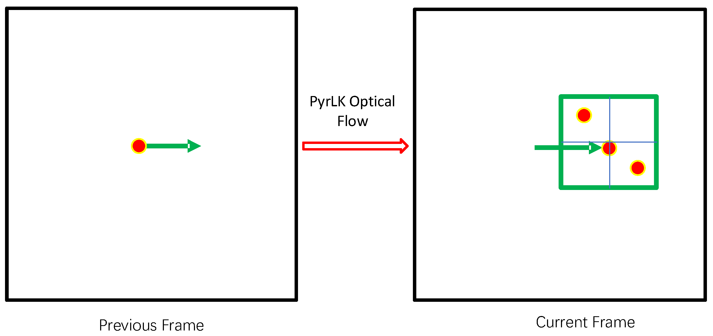
To make full use of time-sequential information in the image, this study proposes to use the Lucas–Kanade optical flow algorithm [31], as illustrated in Figure 5, to track and manage the feature points between frames. It saves the feature point information for a certain period and discards the feature points whose tracking is lost or the tracking time exceeds the threshold. Through this technology, the real-time and accuracy of feature points tracking can be ensured.

The optical flow method is used to calculate the motion information of the object or the motion information of the camera by tracking the motion and correlation of the pixels between adjacent frames. To reduce the consumption of calculations, the optical flow tracking of the feature points between frames in this study is only performed on the feature points of the left image. After tracking, the left image feature is matched to the right-eye image according to the binocular matching of the feature points. During the feature point matching process of binocular stereo vision, if no constraint of any prior information is found, then the feature point in the left image must be globally searched in the right image. The brute force solution method is inefficient. For artificial objects such as satellites, many repetitive textures exist, and such solutions are prone to mismatches. In this research, the epipolar constraint is used to reduce the search range, thereby improving the matching efficiency, and reducing the mismatch rate.

2.4. Feature Point Management

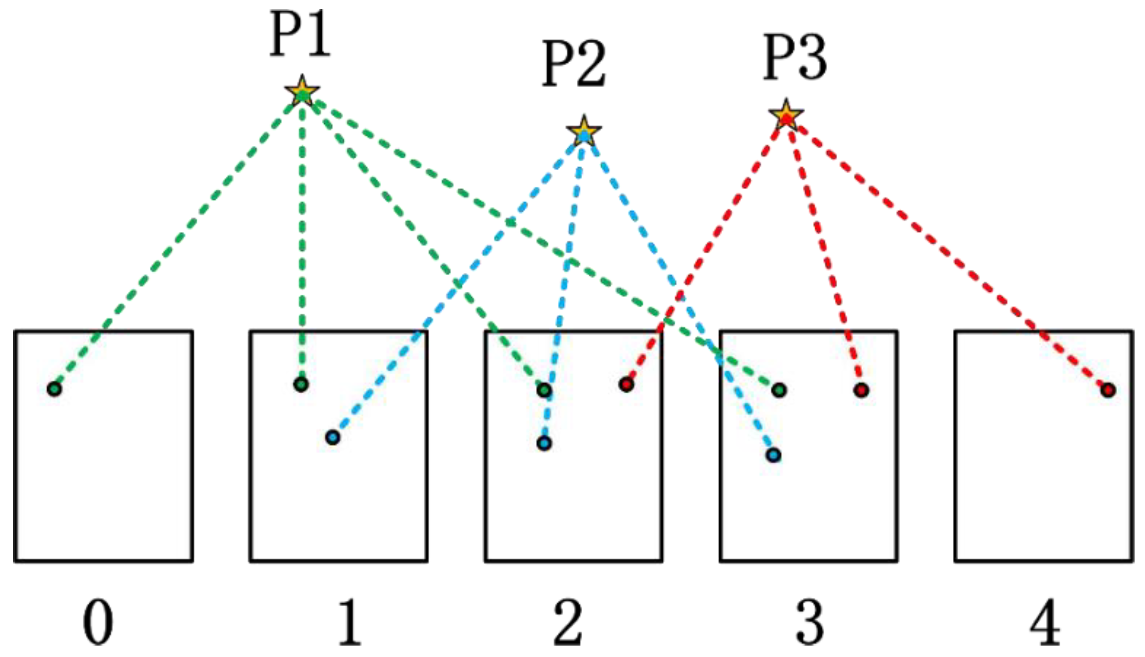
In this subsection, we propose a binocular vision feature point management method, which efficiently balances the calculation efficiency and matching accuracy. To obtain additional representative feature points, we should manage the feature points of consecutive frames after feature point tracking and binocular matching. The management diagram is presented in Figure 6. Feature points P1, P2, and P3 are observed by image frames 0–3, 1–3 and 2–4, respectively.

In the first frame, we detect the FAST corner points in the image and assign their corresponding unique identification number; in the subsequent frames, we must detect new feature points and add them to the feature point sequence. The information of the feature point on each frame includes a unique identification number, response value, survival time at the current moment, pixel coordinates in the left image, pixel coordinates in the right image, 3D position, and 3D velocity of the corresponding spatial point. For example, feature point P1 is observed in four frames (frames 0–3) and loss tracking at the moment of the third frame. The survival time of P1 is 4.

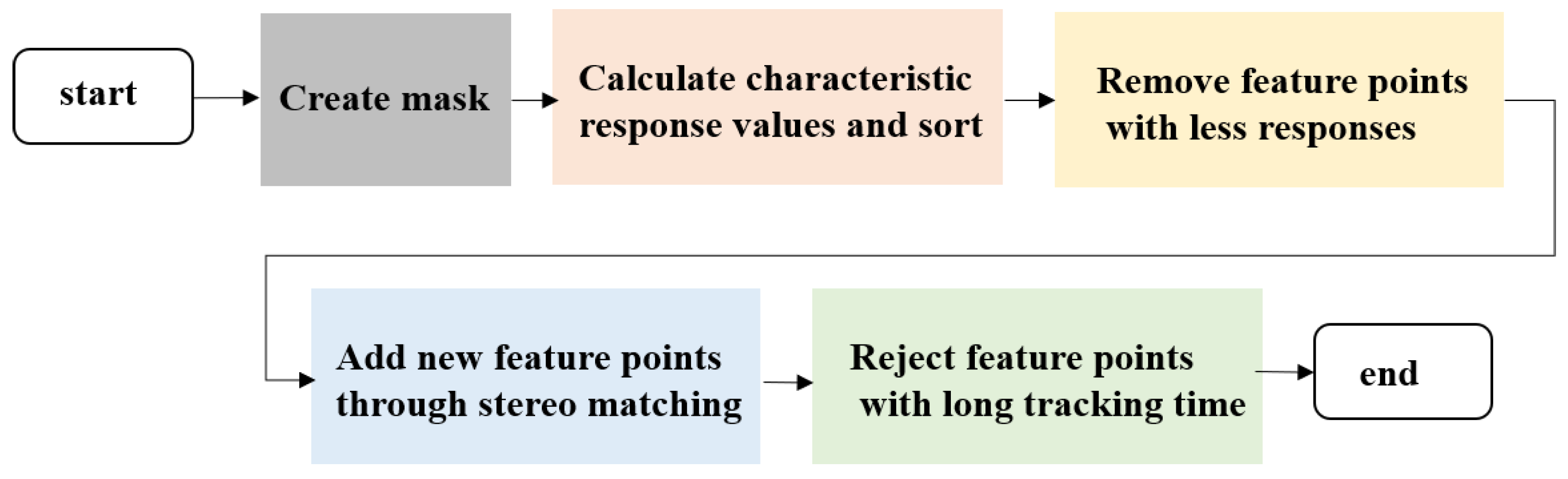
A new frame of image updates the feature point collection through feature point management. The specific process is shown in Figure 7.

The feature point management method can help to express the relationship of the target set accurately. Considering that there may be dense feature areas, a mask is created to filter out the feature points that already exist in the set to avoid repeated detection. The feature point pixel position is ${\left[x,y\right]}^T$, and the mask is an area of $5\times 5$ pixels centered on the feature point pixel. Sorting is performed according to the response values of the feature points. Feature points with small response values are removed. Stereo matching is then conducted. The vacant number in the feature point queue is calculated, where the vacant number is the minimum number of feature points minus the current number of feature points. Subsequently, the vacant number of feature points (sorted) is assigned to the feature point sequence; the corresponding unique identification number is also assigned. Points with more consecutive tracking times are removed. The feature points are sorted according to the number of consecutive tracking. If the number of feature points m exceeds the set maximum number of feature points $n_{max}$, then the previous $\left(n_{max}-m\right)$ points with the most tracking times are removed. Finally, according to the spatial geometric change method, the 3D position and velocity of the characteristic points are used to calculate the relative position, velocity, attitude and angular velocity of the NCT relative to the tracking spacecraft:

$$\overline{y}={\left[\begin{array}{c}{\overline{q}}_{tc}^T {\overline{\omega }}_{tc}^{cT} {\overline{\rho }}_0^T {\overline{\dot{\rho }}}_0^T\end{array}\right]}^T$$

(32)

3. Closed-Loop Simulation Experiment

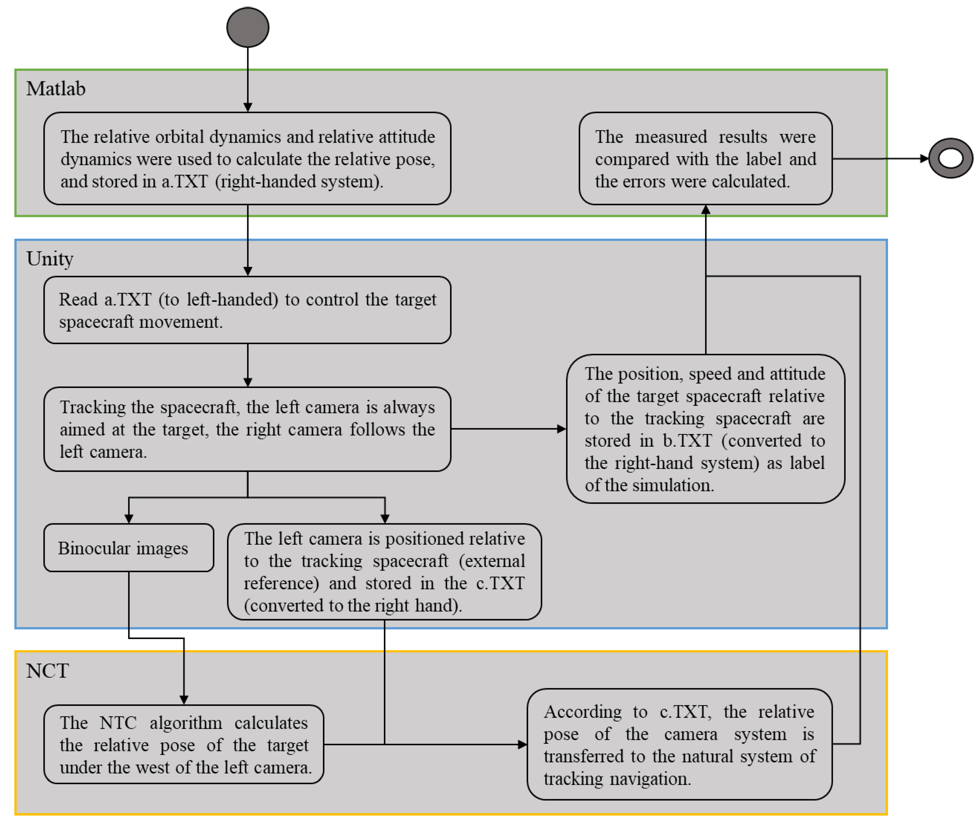
We further verify the relevant algorithm through closed-loop simulation and experiment. The workflow of the closed-loop simulation [6,32] system is illustrated in Figure 8. Three kinds of software are involved in this system, i.e., the MATLAB mathematics software (The MathWorks, Inc., Natick, MA, USA), Unity simulation engine (Unity Technologies, Inc., San Francisco, CA, USA), and the NCT algorithm proposed in this study.

In MATLAB, relative orbit and attitude dynamics are used to calculate the relative pose for a certain period. The results are saved in an a.TXT file. In this part, the relative pose of the spacecraft is expressed in the right-handed coordinate system, to be more specific, LVLH (Local Vertical/Local Horizontal) coordinate system.

Then, the a.txt file is inputted to Unity. Normally, all coordinate systems of the Unity simulation engine are left-handed. To facilitate the operation, we must convert the data to the left-handed system at the beginning and convert them back to the right-handed system before the end of the Unity program. The Unity simulation engine simulates the movement of the target spacecraft based on the relative pose transformed into the left-handed system. To ensure that the target can always be imaged in the binocular camera, we keep the left camera shooting the target. The principle of binocular measurement requires both the left and right camera to see the target. To simplify the design of the spacecraft control system, engineers usually ensured the left side of the binocular shooting at the NCT target. In this case, the other side should be able to see the target under the camera installation structure and baseline constraints. It can also be configured according to the application requirements in the future that the right camera is used for tracking. Three files are output in the Unity program: 1. binocular image, which is used in the NCT algorithm to calculate the relative pose; 2. the rotation and translation of the left camera relative to the tracking spacecraft, expressed in the right-hand system, and stored in a c.TXT file; 3. the relative pose information of the target spacecraft relative to the tracking spacecraft at each moment. This information is also expressed in the right-hand system and saved in a b.TXT file. It is used as the ‘ground truth’ of the simulation system for the subsequent evaluation of system accuracy.

In the NCT autonomous navigation algorithm, the relative position, velocity, attitude and angular velocity of the target spacecraft relative to the left camera system are calculated according to the binocular image. According to the c.txt file, the relative pose information is converted to the references system of the tracking spacecraft. Finally, by subtracting the ground truth from the final solution result, the completion accuracy can be evaluated.

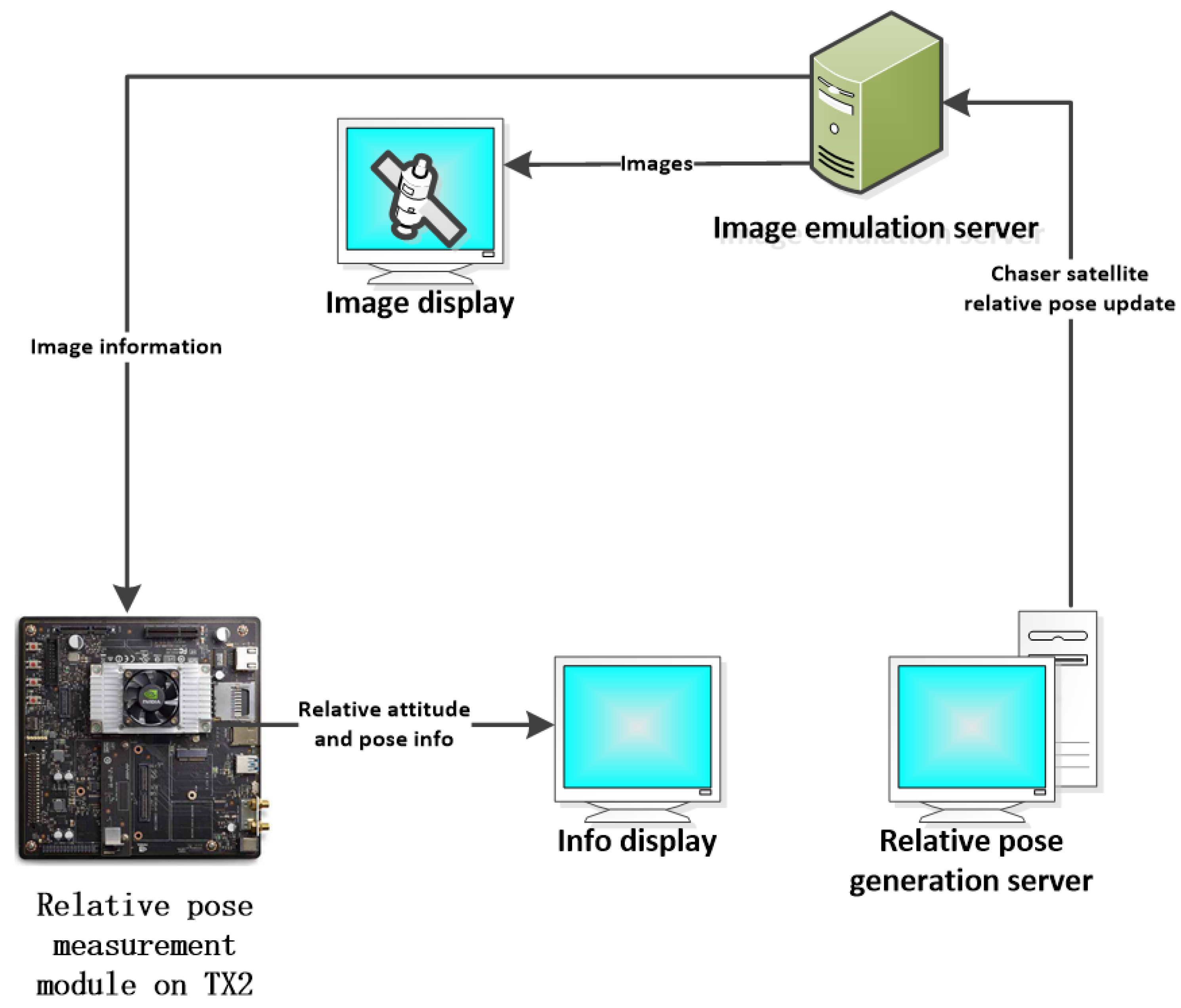
Figure 9 shows the data interaction between different devices in the hardware-in-the-loop (HIL) simulation experiment. The three computers include a relative pose data generation computer, an image data generation computer and a pose calculation computer (embedded platform JetsonTX2). Among them, the relative pose data generation computer is used to generate the relative position and attitude information of the target spacecraft relative to the tracking spacecraft and send it to the image data generation computer. The image data generation computer then controls the relative movement of the two kinds of spacecraft on the basis of the transmitted data and generates images taken by the binocular vision sensor on the tracking spacecraft. The visual images are displayed on the monitor, and finally, the image data are transmitted to the pose calculation computer. The pose calculation computer processes the image, calculates the pose information of the target spacecraft, and displays it on the monitor.

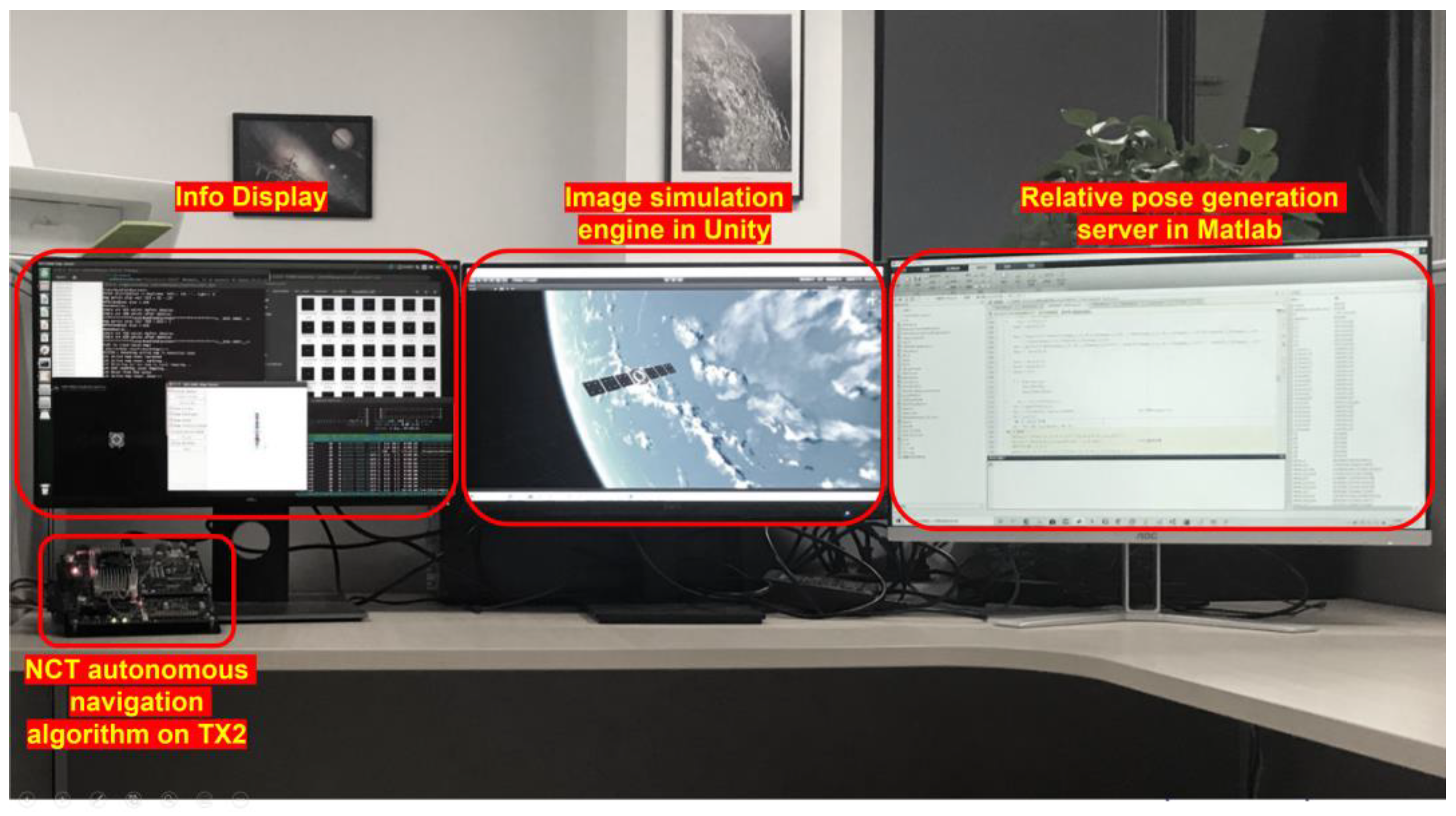
In our closed-loop simulation, we installed MATLAB and Unity in a PC, while NCT autonomous navigation algorithm is deployed in JetsonTX2 supercomputer module, to form the so-called hardware-in-the-loop (HIL) simulation. Figure 10 presents our HIL simulation platform. We involve the JetsonTX2 supercomputer module developed by NVIDIA into the hardware loop simulation platform system. The NVIDIA TX2 module can apply calculations to edge devices and can be used in space missions in the future. TX2 module is made up of industrial-grade components. Compared with traditional spaceborne computing devices, TX2 has the advantage of stronger computing capacity and the disadvantage of huge power consumption and cannot resist space irradiation. Special thermal dissipation and radiation resistance design are required before using this module in space.

3.1. Simulation in Matlab

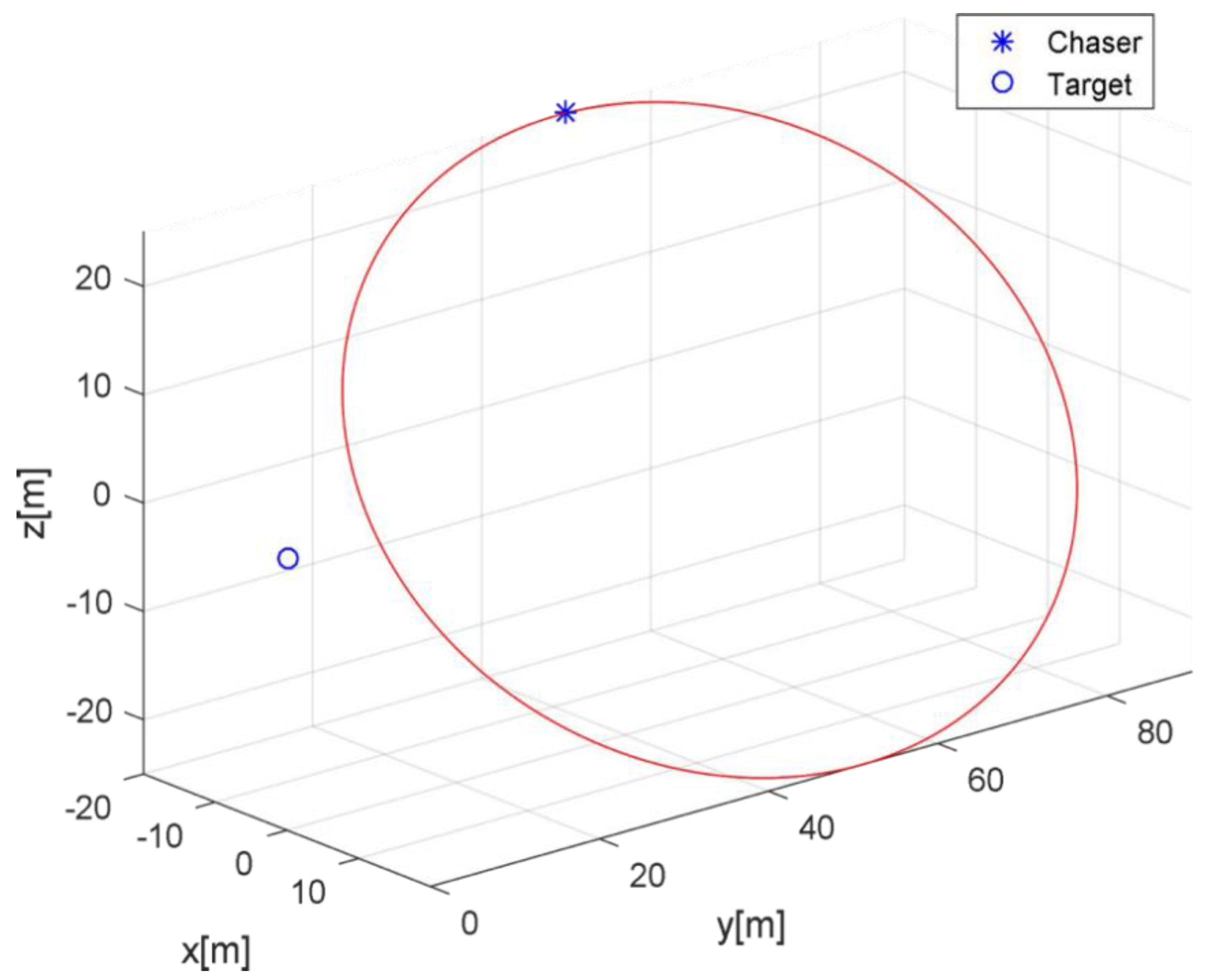
In Matlab, the relative motion is simulated according to the relative motion dynamics model and attitude dynamics model. The initial relative position ${\rho }_0={\left[\begin{array}{ccc}20& -50& -25\end{array}\right]}^T$ m, relative velocity ${\dot{\rho }}_0={\left[\begin{array}{ccc}0& -0.0431& -0.0010\end{array}\right]}^T$ m/s, relative attitude $q_{ct0}={\left[\begin{array}{ccc}0& 0& \begin{array}{cc}0& 1\end{array}\end{array}\right]}^T$ of the two spacecraft, angular velocity ${\omega }_0^t={\left[\begin{array}{ccc}-0.04& -0.06& -0.05\end{array}\right]}^T$ rad/s of the target spacecraft, and angular velocity ${\omega }_0^t={\left[\begin{array}{ccc}0& 0& -0.001078364607802\end{array}\right]}^T$ rad/s of the tracking spacecraft are set. The relative motion trajectory is shown in Figure 11.

3.2. Simulation in Unity

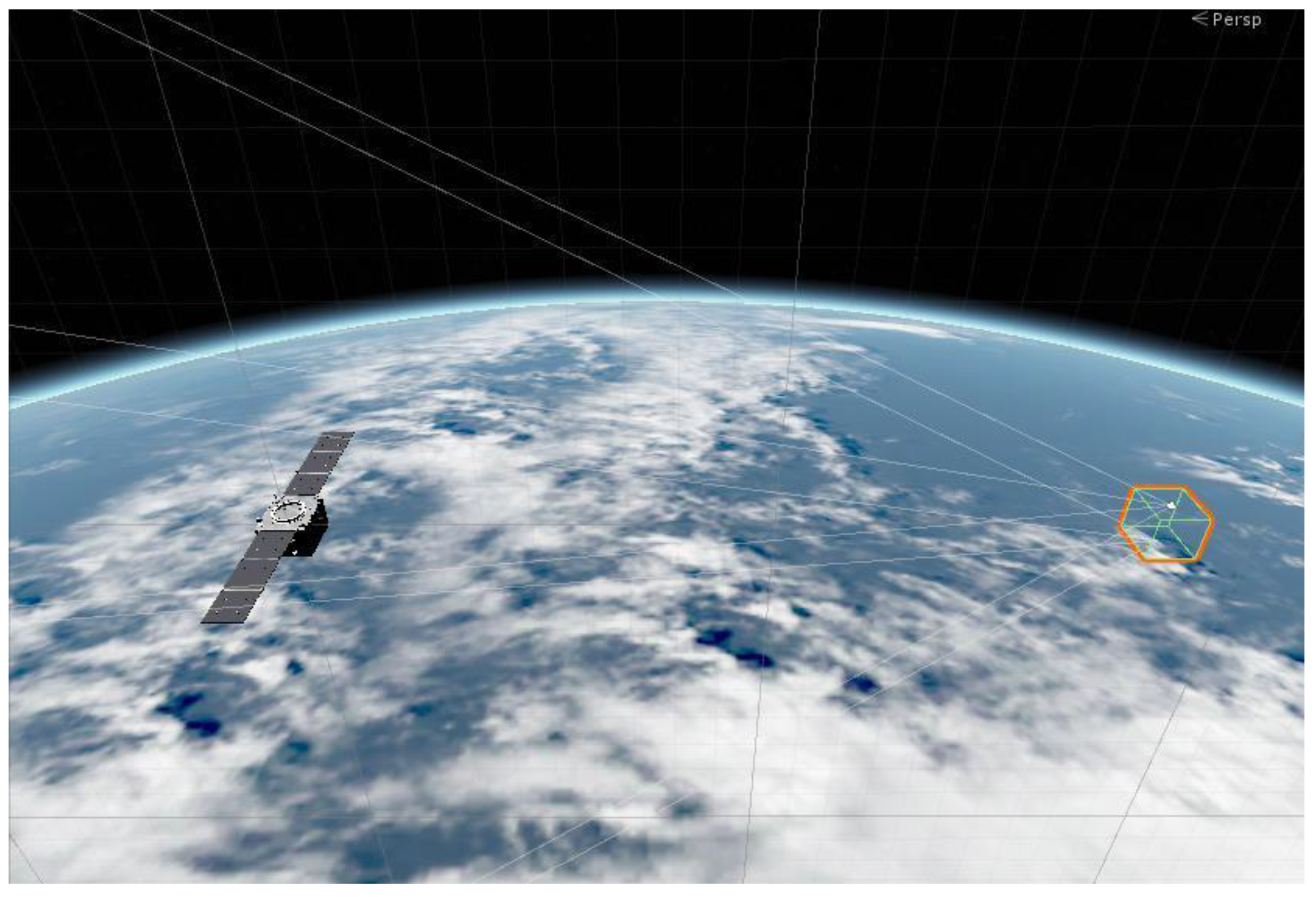
In Unity, the earth model and the environment model are built. Topographic and cloud maps are pasted on the earth model. Unity simulation engine provides four types of lighting sources: directional, point, spot and surface light sources. Our virtual platform simulates the sunshine by using a point light source, which can simulate the shadow part of the earth model. The simulation scene is shown in Figure 12.

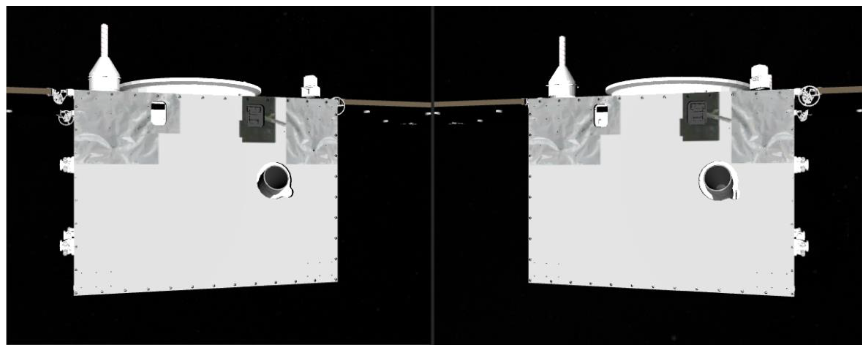
The parameters of the binocular camera in this experiment are presented in

Table 1. Parameters of the simulated binocular cameras.

Parameter	Left Camera	Right Camera
Internal parameters (The first two rows take the unit of pixel, and the third row has no units)	$\left[\begin{array}{ccc}2.0298\times {10}^3& 0.0000& 6.4000\times {10}^2\\ 0.0000& 2.0298\times {10}^3& 6.4000\times {10}^2\\ 0.0000& 0.0000& 1.0000\end{array}\right]$	$\left[\begin{array}{ccc}2.0298\times {10}^3& 0.0000& 6.4000\times {10}^2\\ 0.0000& 2.0298\times {10}^3& 6.4000\times {10}^2\\ 0.0000& 0.0000& 1.0000\end{array}\right]$
Translation vector (mm)	[0.0000 0.0000 0.0000]	[920.00 0.0000 0.0000]

. Radial distortion and tangential distortion of the binocular camera are not considered for the moment. The elements of the rotation matrix of the left camera are all zeros, and the rotation matrix of the right camera is an identity matrix. During the process of simulating the convergent binocular approaching the target spacecraft, the convergent binocular has a baseline of 0.92 m, a field of view of 35°, the left and the right cameras are tilted 10° inwardly and the image resolution is 1024 × 1024.

It can be seen directly from Figure 13 that the convergent binocular system can increase the effective field of view, especially when the chaser spacecraft is closer to the target.

3.3. Calculation in NCT Autonomous Navigation Algorithm

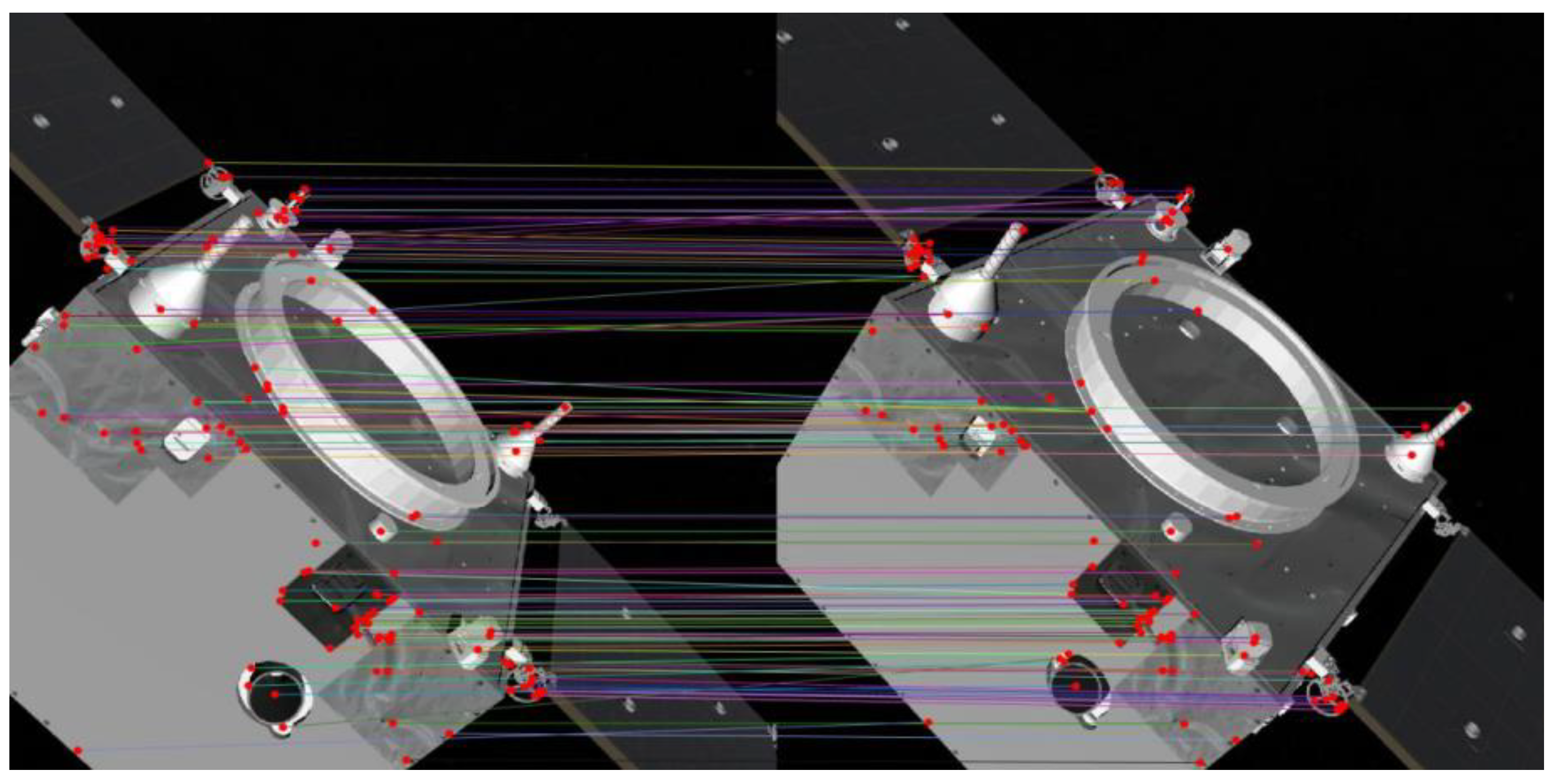
In NVIDIA JetsonTX2 module, the proposed NCT autonomous navigation algorithm performs the feature points extraction, tracking, and matching process. FAST algorithm is used to extract feature points from the binocular camera image. After optical flow tracking, the feature points in the left and right images can be matched by stereo matching. The feature point extraction and matching when the distance to the target is 2.5 m are exhibited in Figure 14. A total of 872 feature points are extracted from the left image, 936 feature points from the right image, and the feature point with the highest response value is selected to match. The red points represent the feature points, and the lines of different colors connect the matched feature point pairs.

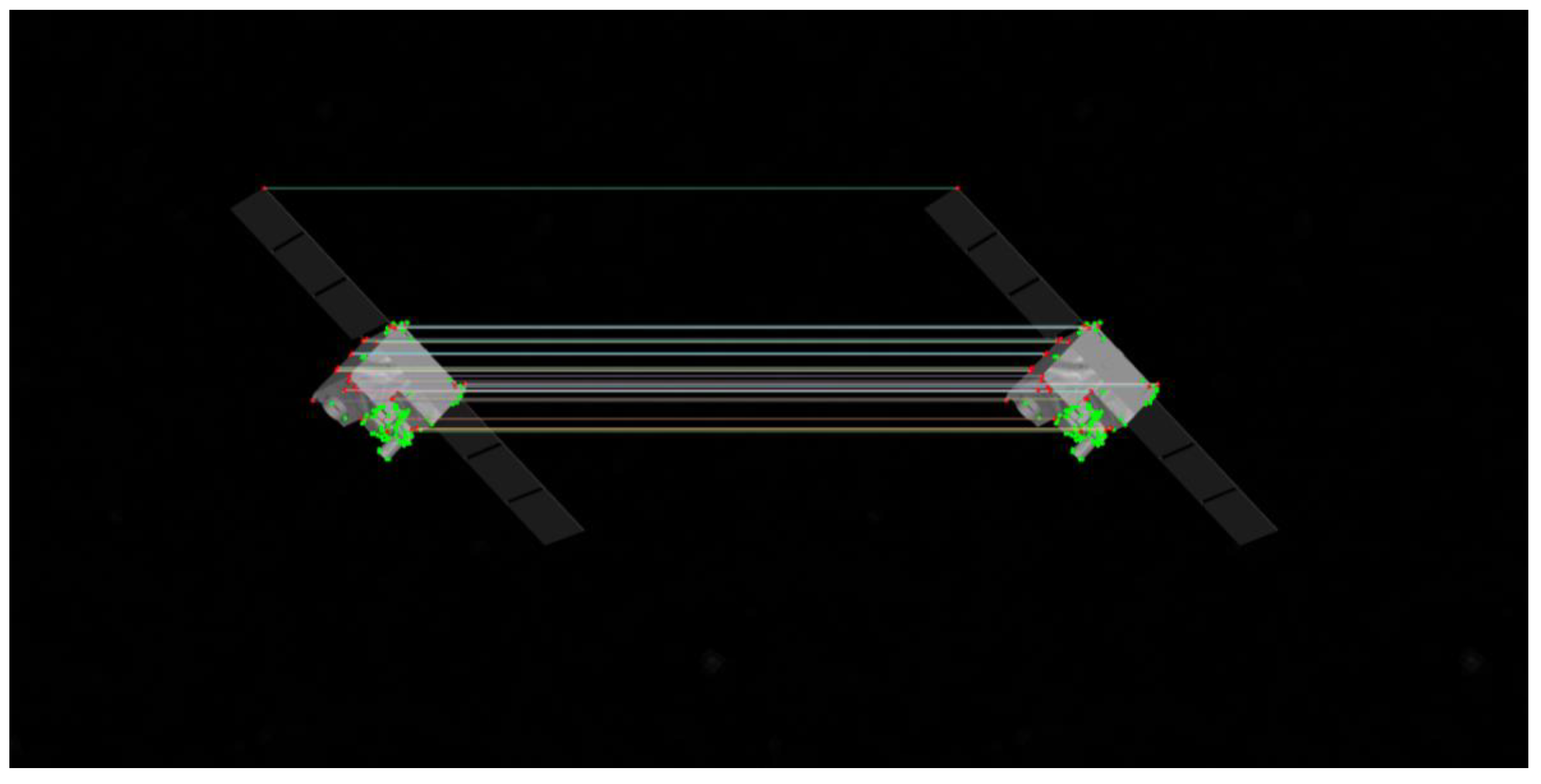
For a new frame of a binocular image, new feature points must be detected. According to the method of feature point management, some feature points with excessively long tracking times and missing feature points are removed, and newly detected feature points with high response values are added, to the feature point sequence. This is shown in Figure 15. The connection line represents the matching of the newly added feature points through the epipolar constraint.

The above experiments suggest that the FAST corner point extraction method can well identify the feature points in the image. The optical flow method can track the feature points of the two frames before and after the matching and accurately reflect the movement process of the target spacecraft. The left and right image feature points of binocular stereo vision can be accurately matched. Feature point management can be performed to maintain the length of the feature point sequence at 120 points, which ensures that the number of calculations is limited and guarantees real-time performance.

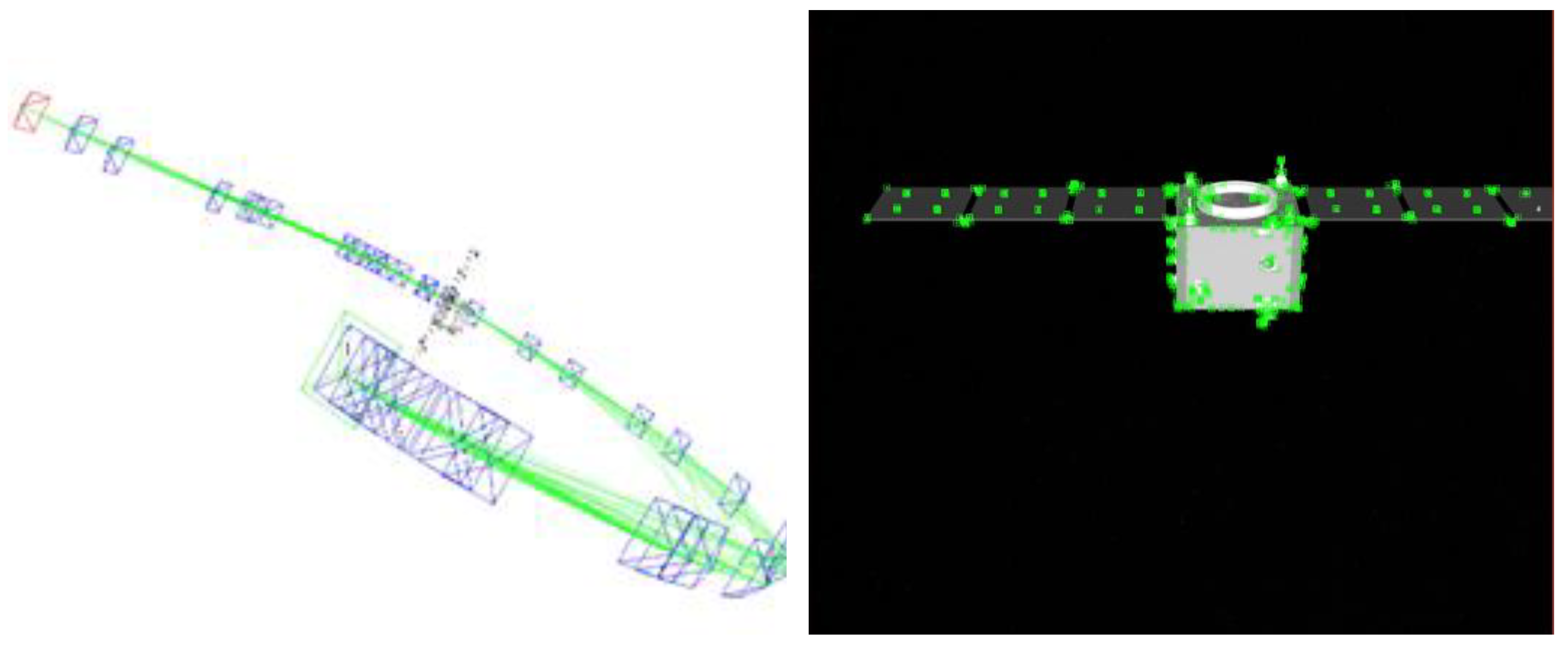
In the NCT autonomous navigation algorithm, the relative position, velocity, attitude, and angular velocity of the target spacecraft relative to the left camera system are calculated according to 120 matched feature points. A more accurate solution can be obtained after sequential EKF filtering using the relative orbit dynamics and the relative attitude dynamics model. While storing the solution result, the camera angle of view and relative trajectory are displayed, as shown in Figure 16. The picture on the left shows the relative motion trajectory of the tracking spacecraft to the target spacecraft. The red box is the position of the tracking spacecraft at the start time. The blue box represents the track of the historical trajectory of the spacecraft. The two ends connected by the green line indicate that the images captured by the cameras at these two locations have a common view relationship. The black point cloud represents the 3D point cloud image created by the binocular vision camera on the target through the extracted feature points. The picture on the right shows the image taken by the left camera of the binocular camera and the feature points extracted in the frame.

4. Experimental Results and Discussion

The NCT autonomous navigation algorithm calculates the relative center of mass position, velocity, relative attitude, and angular velocity. The NCT calculation result is subtracted from the ground truth (output of Unity) to obtain the error result. In this subsection, we will present the closed-loop simulation results and discussion.

4.1. Filter Initiation

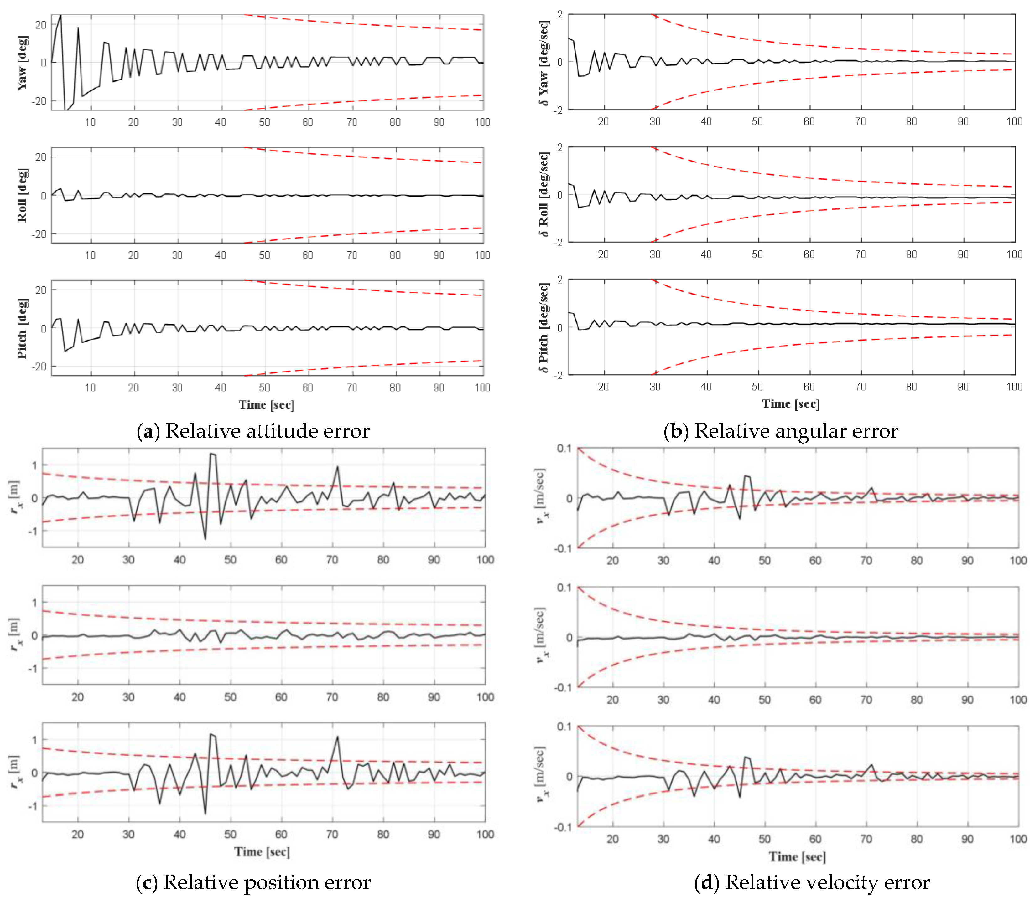
The NCT autonomous navigation algorithm can only calculate the relative position, velocity and attitude at the subsequent time after assuming the relative attitude at the initial time. Therefore, the relative attitude of the target needs to be initialized before sequentially filtering. In our experiment, we use the first 100 frames of binocular observations to initialize the navigation filter.

Figure 17 shows the error result after the initialization of the first 100 frames of interception. The experimental results reveal that the relative attitude and angular velocity can converge quickly after initialization, whereas the relative position and velocity can converge within 90 frames. After convergence, the average relative attitude error is 0.6896°, the average relative angular velocity error is 0.2120°/s, the average relative position error is 0.0316 m and the relative velocity average error is 0.0017 m. It is worth mentioning that the initialization process is usually required if one established a globally consistent coordinate system for the NCT. In practical engineering, the initial value of relative attitude at the initial moment can be obtained from the navigation results of the previous stage. For example, before starting the binocular relative navigation mode, the monocular camera or lidar are also conducting relative navigation, which can ensure that an initial value with smaller error is output to the binocular navigation algorithm. On the other hand, the initialization process is reasonable, not required, if the navigation is performed with respect to an arbitrarily chosen frame attached to the chaser spacecraft. The term ‘arbitrarily chosen’ means re-extracting the coordinate system of the target spacecraft at the beginnings of each stage during the process of orbit service missions. The extraction of the coordinate system of the target spacecraft has been introduced previously. Readers can refer to [14,15,16,17,18].

4.2. Filter Navigation Performance

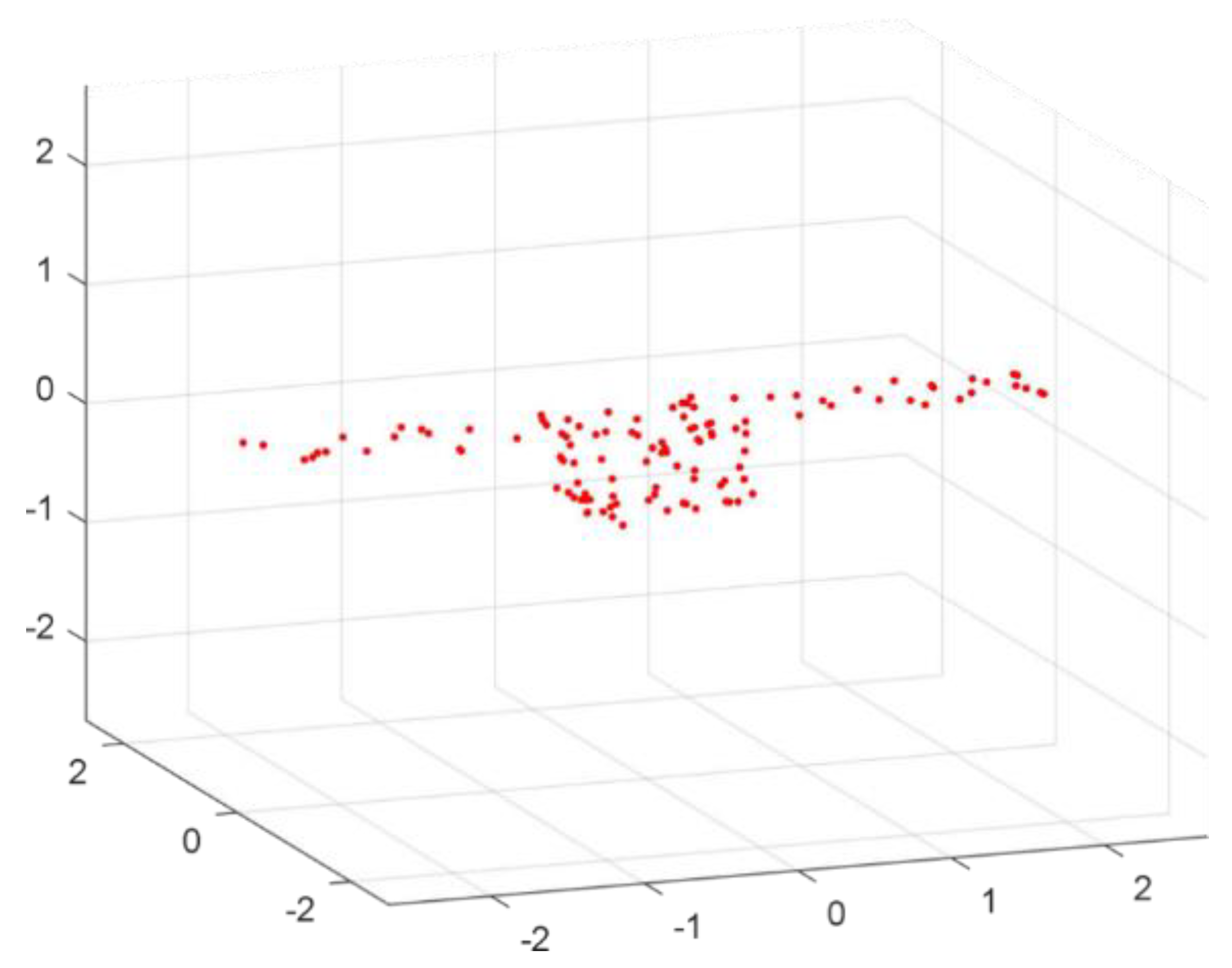
After feature point extraction, tracking, matching and other management operations, the paired feature points reflect a point cloud in three-dimensional space. As illustrated in Figure 18, the red dots indicate the positions of the feature points set in the target spacecraft coordinate system at a particular moment in time.

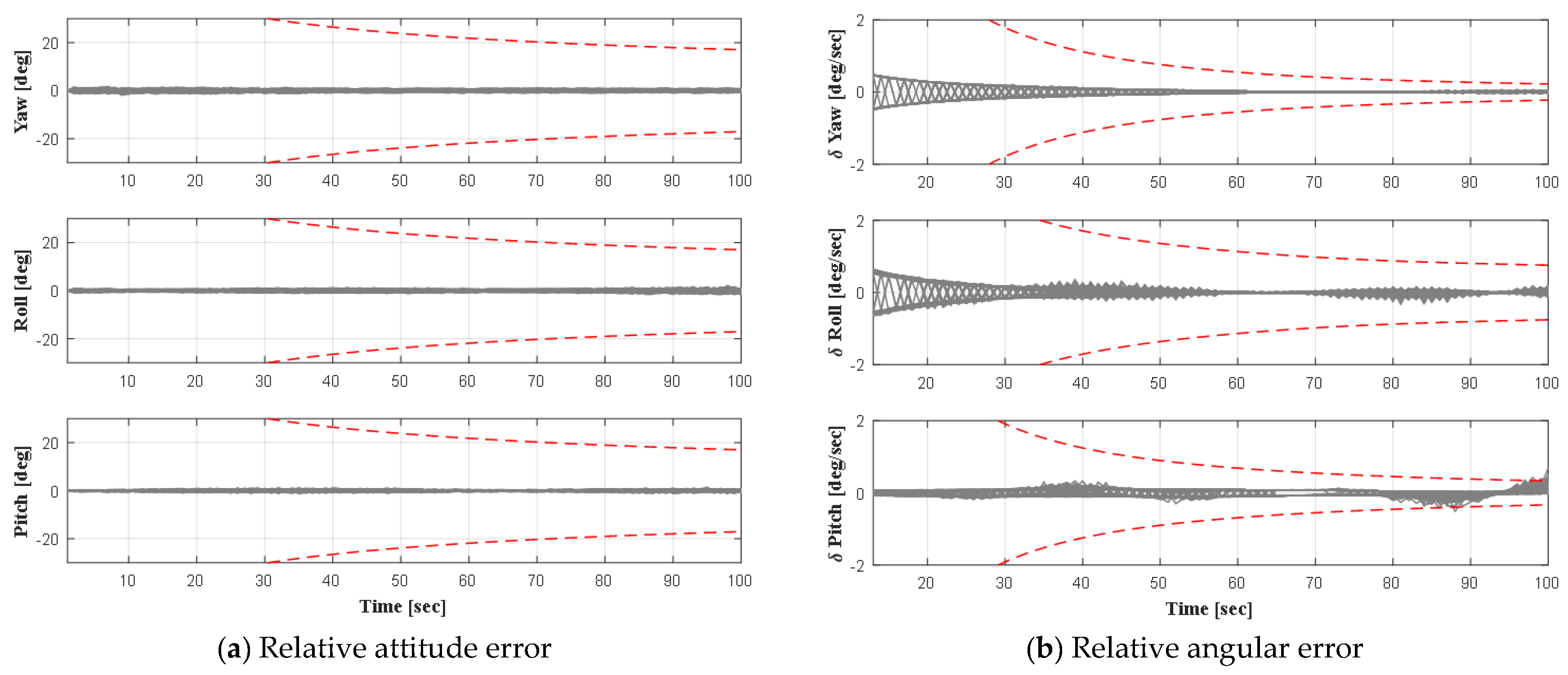
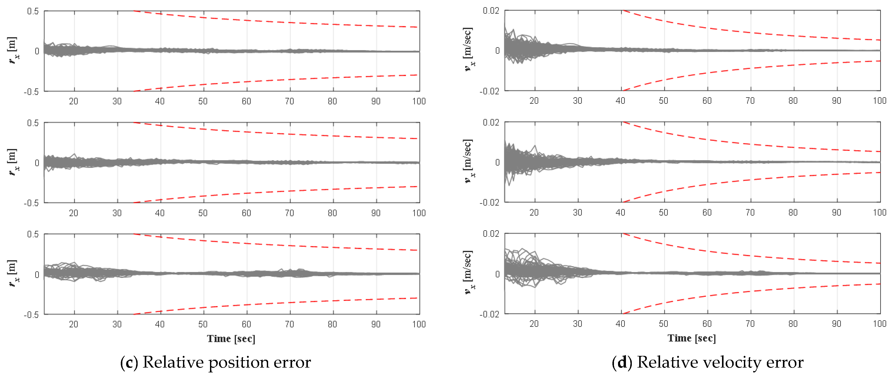
The NCT autonomous navigation algorithm calculates the relative position, velocity, attitude, and angular velocity of the target spacecraft relative to the left camera system according to the pixel coordinates of 120 pairs of matched feature points. A more accurate solution can be obtained after sequential EKF filtering, using the relative orbit dynamics and the relative attitude dynamics model. The initial parameters of the relative motion trajectory simulated by MATLAB are used as the initial values of the EKF. A Monte Carlo simulation is conducted 100 times, and the results after filtering are shown in Figure 19 below, where the red line represents the Kalman filter 3 σ envelope.

The results indicate that our algorithm converges within 40 s. Statistics of the state errors are shown in

Table 2. Statistics of state errors.

State	Statistic	Result
Attitude (deg)	Mean	[0.0238 8.2274 × 10−4 0.0094]
	Standard deviation	[0.4482 0.5480 0.5298]
Angular velocity (deg/s)	Mean Standard deviation	[0.0222 0.0353 0.0030] [0.5400 0.6336 0.2833]
Centroid position (m)	Mean Standard deviation	[0.0033 0.0032 0.0090] [0.1146 0.1157 0.1161]
Centroid position velocity (m/s)	Mean	[0.5471 × 10−4 9.6595 × 10−4 4.2910 × 10−4]
	Standard deviation	[0.0298 0.0308 0.0309]

below.

After convergence, the maximum deviation of the target position error is less than 0.05 m, the maximum deviation of the velocity error is less than 0.002 m/s, the maximum deviation of the Euler angle error is less than 1° and the maximum deviation of the angular velocity error is less than 0.1°/s.

5. Conclusions

The aim of this research is about relative position and attitude estimation of non-cooperative spacecrafts in the last 20 m approaching stage. Based on the binocular vision camera measurement and the relative dynamic model, an autonomous navigation filter is designed to measure the relative pose. The proposed algorithm is verified by virtual simulations. The experimental results show that the algorithm proposed in this paper can accurately complete the positioning and attitude determination of non-cooperative targets. The contributions of this work are as follows: (1) to solve the challenge of the disastrous mismatching of feature points caused by serious repeated textures on the surface of NCTs under complex lighting conditions, an optical flow method is used to track the feature points and match the feature points of the images captured by left and right cameras; (2) a feature point management method is proposed to balance the calculation efficiency and matching accuracy more efficiently; and (3) a navigation filtering algorithm is designed, and the dynamic model is used to optimize the visual measurement results. According to the actual mission profile of a certain type of spacecraft, a virtual simulation closed-loop experimental platform is built to verify the relative navigation algorithm. Finally, the results are compared with the ground truth to analyze the error and verify the feasibility and real-time performance of the algorithm.

This paper provides some technical details for potential on-orbit evasion and on-orbit rescue missions. It is worth mentioning that the approach provided in this paper is only concerned with short-range relative navigation; many other technologies are needed to support the whole range mission. In the future, the autonomous navigation system is also necessary to cooperate with the satellite attitude and orbit control system to realize the on-orbit demonstration task.

References

- Li, W.J.; Cheng, D.Y.; Liu, X.G.; Wang, Y.B.; Shi, W.H.; Tang, Z.X.; Gao, F.; Zeng, F.M.; Chai, H.Y.; Luo, W.B.; et al. On-orbit service (OOS) of spacecraft: A review of engineering developments. Prog. Aerosp. Sci. 2019, 108, 32–120. [Google Scholar] [CrossRef]
- Flores-Abad, A.; Ma, O.; Pham, K.; Ulrich, S. A review of space robotics technologies for on-orbit servicing. Prog. Aerosp. Sci. 2014, 68, 1–26. [Google Scholar] [CrossRef] [Green Version]
- Wang, D.; Hou, B.; Wang, J.; Ge, D.; Li, M.; Xu, C.; Zhou, H. State estimation method for spacecraft autonomous navigation: Review. Hangkong Xuebao Acta Aeronaut. Astronaut. Sin. 2021, 42. [Google Scholar]
- Cassinis, L.P.; Fonod, R.; Gill, E. Review of the robustness and applicability of monocular pose estimation systems for relative navigation with an uncooperative spacecraft. Prog. Aerosp. Sci. 2019, 110, 100548. [Google Scholar] [CrossRef]
- Bordeneuve-Guibé, J.; Drouin, A.; Roos, C. Advances in Aerospace Guidance, Navigation and Control; Springer: Berlin/Heidelberg, Germany, 2015. [Google Scholar]
- Xu, W.; Liang, B.; Li, C.; Liu, Y.; Wang, X. A modelling and simulation system of space robot for capturing non-cooperative target. Math. Comput. Model. Dyn. Syst. 2009, 15, 371–393. [Google Scholar] [CrossRef]
- Leinz, M.R.; Chen, C.-T.; Beaven, M.W.; Weismuller, T.P.; Caballero, D.L.; Gaumer, W.B.; Sabasteanski, P.W.; Scott, P.A.; Lundgren, M.A. Orbital Express Autonomous Rendezvous and Capture Sensor System (ARCSS) flight test results. In Proceedings of the Sensors and Systems for Space Applications II, Orlando, FL, USA, 17–18 April 2008; Volume 6958. [Google Scholar]
- Bodin, P.; Larsson, R.; Nilsson, F.; Chasset, C.; Noteborn, R.; Nylund, M. PRISMA: An in-orbit test bed for guidance, navigation, and control experiments. J. Spacecr. Rocket. 2009, 46, 615–623. [Google Scholar] [CrossRef]
- Woods, J.O.; Christian, J.A. Lidar-based relative navigation with respect to non-cooperative objects. Acta Astronaut. 2016, 126, 298–311. [Google Scholar] [CrossRef]
- Qiu, Y.; Guo, B.; Li, C.; Liang, B. Study on Federal Filter of Relative Navigation for Non-cooperative Spacecraft. J. Astronaut. 2009, 30, 2206–2212. [Google Scholar]
- Aghili, F.; Su, C.-Y. Robust Relative Navigation by Integration of ICP and Adaptive Kalman Filter Using Laser Scanner and IMU. IEEE/ASME Trans. Mechatron. 2016, 21, 2015–2026. [Google Scholar] [CrossRef]
- Augenstein, S.; Rock, S.M. Improved frame-to-frame pose tracking during vision-only SLAM/SFM with a tumbling target. In Proceedings of the IEEE International Conference on Robotics and Automation, Shanghai, China, 9–13 May 2011; pp. 3131–3138. [Google Scholar]
- Ruel, S.; Luu, T.; Berube, A. Space Shuttle Testing of the TriDAR 3D Rendezvous and Docking Sensor. J. Field Robot. 2012, 29, 535–553. [Google Scholar] [CrossRef]
- Lichter, M.D. Shape, Motion, and Inertial Parameter Estimation of Space Objects using Teams of Cooperative Vision Sensors; Massachusetts Institute of Technology: Cambridge, MA, USA, 2005. [Google Scholar]
- Setterfield, T.P.; Miller, D.W.; Leonard, J.J.; Saenz-Otero, A. Mapping and determining the center of mass of a rotating object using a moving observer. Int. J. Robot. Res. 2018, 37, 83–103. [Google Scholar] [CrossRef]
- Tweddle, B.E.; Setterfield, T.P.; Saenz-Otero, A.; Miller, D.W.; Leonard, J.J. Experimental Evaluation of On-board, Visual Mapping of an Object Spinning in Micro-Gravity aboard the International Space Station. In Proceedings of the IEEE/RSJ International Conference on Intelligent Robots and Systems (IROS), Chicago, IL, USA, 14–18 September 2014; pp. 2333–2340. [Google Scholar]
- Lyzhoft, J.; Wie, B. New image processing algorithm for terminal guidance of multiple kinetic-energy impactors for disrupting hazardous asteroids. Astrodynamics 2019, 3, 45–59. [Google Scholar] [CrossRef]
- Gong, B.; Li, W.; Li, S.; Ma, W.; Zheng, L. Angles-only initial relative orbit determination algorithm for non-cooperative spacecraft proximity operations. Astrodynamics 2018, 2, 217–231. [Google Scholar] [CrossRef]
- Determination, A.; Target, C. A New Method of Relative Position and Attitude Determination for Non-Cooperative Target. J. Astronaut. 2011, 32, 516–521. [Google Scholar]
- Segal, S.; Carmi, A.; Gurfil, P. Stereovision-based estimation of relative dynamics between noncooperative satellites: Theory and experiments. IEEE Trans. Control. Syst. Technol. 2014, 22, 568–584. [Google Scholar] [CrossRef]
- Pesce, V.; Lavagna, M.; Bevilacqua, R. Stereovision-based pose and inertia estimation of unknown and uncooperative space objects. Adv. Sp. Res. 2017, 59, 236–251. [Google Scholar] [CrossRef]
- Feng, Q.; Zhu, Z.H.; Pan, Q.; Hou, X. Relative State and Inertia Estimation of Unknown Tumbling Spacecraft by Stereo Vision. IEEE Access 2018, 6, 54126–54138. [Google Scholar] [CrossRef]
- K, S.-G.; Crassidis, J.L.; Cheng, Y.; Fosbury, A.M.; Junkins, J.L. Kalman Filtering for Relative Spacecraft Attitude and Position Estimation. J. Guid. Control Dyn. 2011, 32, 516–521. [Google Scholar]
- Watanabe, Y.; Johnson, E.N.; Calise, A.J. Optimal 3-D guidance from a 2-D vision sensor. In Proceedings of the Collection of Technical Papers—AIAA Guidance, Navigation, and Control Conference, Providence, RI, USA, 16–19 August 2004; Volume 1. [Google Scholar]
- Julier, S.J.; Uhlmann, J.K. New Extension of the Kalman Filter to Nonlinear Systems. In Proceedings of the Signal Processing, Sensor Fusion, and Target Recognition VI, Orlando, FL, USA, 21–24 April 1997; Volume 3068. [Google Scholar]
- Feng, Q.; Liu, Y.; Zhu, Z.H.; Hu, Y.; Pan, Q.; Lyu, Y. Vision-Based Relative State Estimation for A Non-Cooperative Target. In Proceedings of the 2018 AIAA Guidance, Navigation, and Control Conference, Kissimmee, FL, USA, 8–12 January 2018. [Google Scholar]
- Wahba, G. A least squares estimate of satellite attitude. SIAM Rev. 1965, 7, 409. [Google Scholar] [CrossRef]
- Markley, F.L. Fast quaternion attitude estimation from two vector measurements. J. Guid. Control Dyn. 2002, 25, 411–414. [Google Scholar] [CrossRef] [Green Version]
- Viswanathan, D. Features from Accelerated Segment Test (FAST). In Proceedings of the 10th workshops on Image Analysis for Multimedia Interactive Services, London, UK, 6–9 May 2009. [Google Scholar]
- Song, X.; Yang, L.; Wu, Y.; Liu, Z. A New Depth Measuring Method for Stereo Camera Based on Converted Relative Extrinsic Parameters. In Proceedings of the International Symposium on Photoelectronic Detection and Imaging 2013: Imaging Sensors and Applications, Beijing, China, 25–27 June 2013; Volume 8908. [Google Scholar]
- Karthika Pragadeeswari, C.; Yamuna, G.; Yasmin Beham, G. A robust algorithm for real time tracking with optical flow. Int. J. Innov. Technol. Explor. Eng. 2019, 9, 887–892. [Google Scholar] [CrossRef]
- Turner, A.J. An Open-Source Extensible Spacecraft Simulation and Modeling Environment Framework. Master’s Thesis, Virginia Polytechnic Institute and State University, Blacksburg, VA, USA, 2003. [Google Scholar]
Figure 1.
Typical non-cooperative spacecraft on-orbit service mission.
Figure 2.
The overall algorithm design scheme for relative pose measurement.
Figure 3.
Feature points of the target spacecraft.
Figure 4.
Principle of convergent binocular stereo vision measurement.
Figure 5.
The optical flow algorithm is performed on the feature points tracking procedure.
Figure 6.
Feature point management method.
Figure 7.
Feature point management algorithm flow chart.
Figure 8.
The overall process of the simulation experiment system.
Figure 9.
Configuration of hardware-in-the-loop (HIL) simulation platform. NCT autonomous navigation algorithm is deployed on a pose calculation computer, i.e., NVIDIA JetsonTX2 (NVIDIA Corporation, Inc., Santa Clara, CA, USA) module.
Figure 10.
Hardware-in-the-loop (HIL) simulation platform.
Figure 11.
Simulation of the relative motion trajectory.
Figure 12.
Simulation scene.
Figure 13.
Convergence binocular images simulated from Unity (left: from the left camera, right: from the right camera).
Figure 14.
Feature matching based on convergent binocular stereo vision.
Figure 15.
Feature management. The green points are feature points that have been detected in history and can be tracked in this frame. The red points are newly detected feature points and added to the feature point sequence.
Figure 16.
Visualization of pose information and image with feature points extracted in the frame.
Figure 17.
Error analysis after the initialization of the first 100 frames of interception.
Figure 18.
The positions 120 pairs of feature points in the target spacecraft coordinate system.
Figure 19.
Experimental results of the relative attitude, angular velocity, position, and velocity.