Multisatellite Flyby Inspection Trajectory Optimization Based on Constraint Repairing

Abstract

With the rapid development of on-orbit services and space situational awareness, there is an urgent demand for multisatellite flyby inspection (MSFI) that can obtain information about a large number of space targets with little fuel consumption in a short time. There are two kinds of constraints, namely inspection constraints (ICs) at each flyby point and transfer process constraints (TPCs) in the actual mission. Further considering the influence of discrete and continuous variables such as inspection sequence, time, and maneuver scheme, it is complex and difficult to solve MSFI. To optimize it efficiently, the task flow and the problem model are defined firstly. Then, the algorithm framework based on constraint repairing is given, which contains repair methods of the ICs and the TPCs. Finally, the proposed method is compared with the nonrepair optimization method in two numerical examples. The results indicate that when the constraints are hard to meet, it is better and more efficient than the nonrepair method.

1. Introduction

In the recent half-century, on-orbit services (OOSs) have been widely used in space stations, space shuttles, space telescopes, and other items, which have provided human beings huge economic value and science rewards [1]. Besides, autonomous OOSs have been gradually applied in the recent several years, such as on-orbit refueling and on-orbit inspection missions, which have preliminarily shown application prospects [1,2]. The number of space targets is increasing rapidly, and providing effective on-orbit services for a large number of satellites is a great challenge for space agencies of all countries.

Multisatellite flyby inspection (MSFI) refers to the fact that a service satellite (SS) or multiple SSs perform the orbital transfer in a short period and fly by multiple target satellites at close range to obtain target images and radio signal characteristics and other information to provide support and help for space situational awareness and subsequent OOSs. Compared with the approach of close inspection through coplanar rendezvous, MSFI can not only obtain information of more targets through fast flyby inspection on different planes but also save propellant and time, which is more suitable for the needs of close inspection of satellite groups. To obtain clear image information, it is required that the inspection points have good illumination conditions and the line-of-sight rotation rate be within a certain range, which can be collectively referred to as the inspection constraints (ICs) at each flyby point. In the orbital transfer process, the size of a single maneuver is limited by the engine capacity, and the orbital height cannot be lower than the lowest limit of low earth orbit (LEO), which are collectively referred to as transfer process constraints (TPCs). Due to the coupling effect of the ICs and TPCs, the trajectory optimization problem of MSFI is different from the trajectory optimization problems of multisatellite rendezvous and unconstrained multisatellite flyby, which have been studied extensively. The problem becomes complex and difficult to solve after considering the comprehensive influence of discrete and continuous variables such as inspection order, time, and maneuver scheme.

If the current position and velocity of the SS and the information of the target to be flown by are known and the orbit plane intersection inspection is adopted, the SS does not need to adjust the orbit plane. At this time, the position of the flyby point is determined, and the orbit maneuver solution is essentially a two-point boundary value problem (TPBVP). The Lambert problem, as a classical TPBVP, has been a hot topic for many years. The constrained Lambert problem is an important research direction of the TPBVP. Zhang et al. characterized the minimum perigee and maximum apogee constraints as the constraints of semimajor axis iterative variables and then obtained the feasible revolution range in the multirevolution algorithm, which can reduce the number of cycles to be evaluated [3]. Huang et al. characterized apogee and perigee height constraints as the lateral component range of eccentricity vector, and the solution of multirevolution transfer can be selected in advance to meet the constraints [4]. Thompson et al. made the dynamic transformation of height constraints of apogee and perigee and determined the input direction of flight, transfer time, and cycle range by semimajor axis versus transfer time graph [5]. According to the demand of Moon-to-Earth transfer, Luo et al. effectively transformed the dynamic characterization of the original Lambert problem for the quasi-Lambert problem with limited departure flight-direction angle but free transfer angle and gave a fast iterative solution [6]. Karthikeyan et al. proposed a two-pulse maneuver strategy to meet the constraints of reentry terminal time and flight-direction angle based on the Lambert problem [7]. Aiming at the constraint of orbital maneuvering pulse size, Shirazia et al. characterized the multipulse rendezvous problem as a multisegment two-point boundary value problem [8].

For other constrained TPBVPs, Thompson et al. proposed a tangent guidance method with constrained initial or terminal flight direction angle according to the safety requirements of rendezvous and solved it by numerical iteration [9]. Taur et al. constructed the optimal rendezvous/interception primer vector method with path constraints by using the variational method to deal with the constraints of perigee and apogee [10]. Zhang et al. derived the analytical solution of tangent guidance and gave the existence condition of the solution [11]. Zhang et al. derived the partial derivative analytical model of the influence of orbital maneuver along the track on the illumination conditions and the trajectories of the subsatellite point based on the J2 relative dynamics equation and revealed the law of the influence on the fast and slow diffusion directions [12,13]. Liu et al. studied the optimal pulse guidance law considering the impact angle constraint of the intercept terminal [14]. Xie et al. considered the constraints of pulse time, pulse component size, and terminal position and derived the first-order necessary condition of minimum velocity increment by using the variational method [15].

The above studies mainly consider the requirements of perigee and apogee height and terminal velocity direction, and some studies consider the constraint of single maneuver pulse size. The optimization of a single flyby inspection trajectory is the underlying support of MSFI. The single flyby time needs to be as short as possible, and the excellent results often appear in the boundary of constraint satisfaction and conflict. The way of constraint processing directly affects the effect and efficiency of multisatellite problem-solving.

The problem of multisatellite flyby belongs to the problem of multisatellite access, and a similar problem is the problem of multisatellite rendezvous. For multisatellite rendezvous, there are three different modes: one to many (O2M), many to many (M2M), and peer to peer (P2P). They are rendezvous modes of one SS or multiple SSs and multiple target satellites and rendezvous mode of each satellite. The first is O2M mode. Hudson et al. and Zhang et al. studied the OOS problem [16,17]. Taking the optimal speed increment or the maximum task revenue as the task index, the optimal sequence was obtained by using the optimization algorithm. Zhang et al. also considered constraints such as illumination. Barea et al. and Zhao et al. studied the problem of large-scale space debris removal, aiming at maximizing mission revenue, and obtained rendezvous sequences and actual trajectories that meet both time and energy constraints [18,19]. The second is M2M mode. Li et al. studied the on-orbit refueling problem with the background of the fuel station and refueling spacecraft [20], optimized the task allocation and refueling sequence, and obtained the on-orbit refueling scheme meeting the constraints of time and carrying capacity. Zhang et al. and Zhu et al. considered the location of the refueling station and the cost of an open refueling station; ant colony algorithm or clustering algorithm was used to determine the location and number of fuel stations to meet the on-orbit refueling task constraints [21,22]. Guo et al. considered multiple-satellite deployment problems and used genetic algorithms and sequential quadratic programming to optimize the transfer orbits [23]. The third is the P2P mode. Yu et al. proposed a two-stage planning strategy to apply to the P2P mode, considering the complex constraints of communication time window and illumination [24]. Du et al. took the distributed on-orbit refueling as the research object, transformed the problem into a graph matching problem, and used graph theory algorithm and genetic algorithm to solve it [25].

For the problem of the multisatellite flyby, coplanar maneuver and out-of-plane flyby are usually used to visit the target spacecraft. Zhang et al. gave the necessary and sufficient conditions for a single spacecraft to fly by three Walker constellation satellites in different planes without orbital maneuver [26]. Zhou et al. studied the close-range observation mission of multisatellite flyby based on coplanar maneuver; proposed the method of perigee maneuver to fly by different targets; and optimized the flying sequence [27], task time, and maneuver strategy with a two-level optimization model. Based on the work of Zhou et al., Zhu et al. put forward the strategy of two-tangent-impulse maneuver [28], which made the maneuver position not only limited to the perigee, and completed the mission of out-of-plane flyby. Zhao Z. studied the MSFI mission based on coplanar maneuver strategy and hybrid-encoding genetic algorithm (HEGA) but did not consider the complex constraints such as illumination [29]. Ma N. proposed the strategy of backward phase maneuver, where a single mission satellite flew by target satellites on different orbit planes and completed the task of traversal access to the Walker constellation [30]. Peng et al. used greedy search and multiround planning method to obtain the mission scheme of MSFI and compared it with the traditional optimization method [31].

For a single flyby inspection mission, some researchers do not consider the ICs. Even if the ICs are considered, the inspection window is often predicted and screened based on the Hohmann-like maneuver in engineering, which discards a large number of inspection opportunities that are considered as infeasible due to ineffective constraint processing, thus affecting the effect of MSFI trajectory optimization [31]. In the mission of multisatellite flyby or rendezvous, the combination of evolutionary algorithm and penalty function is used to solve the problem, which leads to low efficiency and has difficulty in finding a feasible solution when the existing constraints are difficult to meet [17,29]. Only considering the O2M MSFI problem with coplanar maneuvers, to obtain the feasible solution satisfying the constraints in a short time and obtain a better optimization effect, this paper proposes an MSFI trajectory optimization method based on constraint repairing and compares it with the nonrepair optimization method. Comparing with the existing work [31], the main contributions of this article are as follows: Firstly, in the current research of constrained TPBVPs, this paper derives the repair range satisfying the single flyby inspection constraints through theoretical derivation, which improves the constraint process efficiency and provides support for the subsequent constraint repairing. Secondly, in the current research of multisatellite flyby or rendezvous problems with multiple constraints, such as the MSFI problems, we propose a constraint repairing method to increase feasible solution numbers and to improve optimization effects and efficiency compared with the method without repairing, especially when the constraints are hard to meet. The specific sections of this paper are arranged as follows: Section 2 is the task flow, problem model, and solution algorithm. Section 3 gives two examples to verify the proposed method and compares the proposed algorithm with the nonrepair optimization method. Section 4 gives the conclusion and prospects of the future research direction.

2. Mission Description and Trajectory Optimization Method

2.1. Task Flow of MSFI Using Coplanar Maneuvers

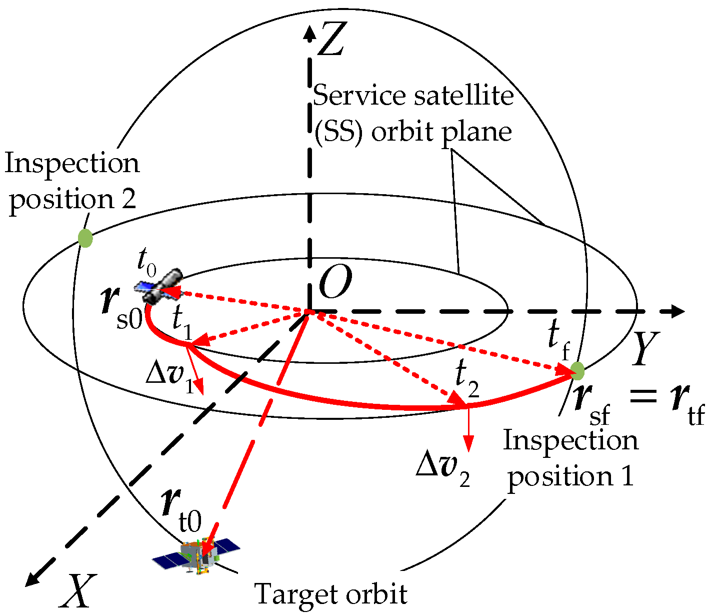
In this article, there is only one SS; that is, we only consider the O2M MSFI problem. As shown in Figure 1, when the target passes through the orbital plane of the SS, we define this time as the candidate end time of the mission. Each revolution of the target will intersect with the orbit plane of SS at two positions, and we generally select one position as the end time of the mission. The selection principles are as follows: If one position is in the Earth’s shadow, then we will select another one. If both positions are out of the shadow, we will choose the position closest to the target or try to keep the position close to the previous one. The calculation formula of the candidate end time of the task is shown in [29] and is not described in detail here.

The platform only needs coplanar maneuvers, and at the end of each transfer, it can fly by the target in a short distance. The orbit transfer process is shown in Figure 1. The SS starts from the initial position, executes two coplanar maneuvers at t₁ and t₂, respectively, and conducts close-range flyby inspection on the target at the end of the transfer. After flying by and inspecting one target satellite, the SS continues to perform coplanar maneuver orbit transfer and inspects the next target until all the target satellites are inspected.

2.2. Mathematical Model of Problem

For the mathematical model of the MSFI trajectory optimization problem, it is necessary to clarify the optimization variables, optimization objectives, and constraints, which are described below. The optimization variables generally include the sequence variables of inspecting multiple target satellites; the time of completing each inspection mission, that is, the number of orbital revolutions for target satellite flight when inspecting each target; and the maneuver time, size, and direction variables of inspecting each target satellite. The optimized objective function is to minimize the total propellant consumption, as shown in Equation (1).

$$\min J=M_0(1-\exp (-{\displaystyle \sum _{i=1}^n{\displaystyle \sum _{j=1}^2\Vert \Delta v_{ij}\Vert }}/(I_{\mathrm{s}}{g}_0)))$$

(1)

where $M_0$ is the initial mass, $\Delta v_{ij}$ is the jth maneuver to inspect the ith target, $n$ is the number of target satellites, $g_0$ is the gravitational acceleration at sea level, and $I_{\mathrm{s}}$ is the specific impulse of the engine.

Constraints include the ICs and TPCs for each target satellite. The ICs include relative velocity constraints and constraints of the angle between sunlight and line-of-sight (ASL). The TPCs include maneuver size constraints and perigee height constraints. The details are listed as follows:

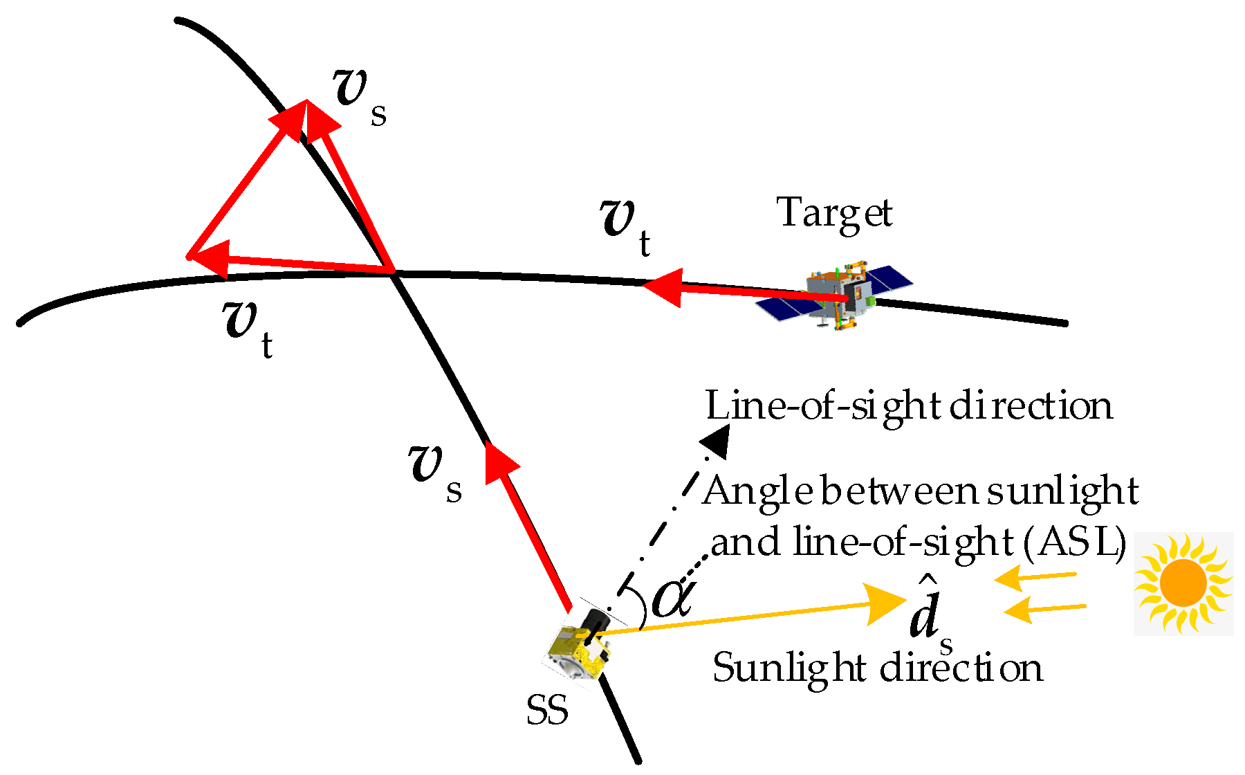
(1) ASL constraints: The optical imaging equipment requires that the sunlight cannot appear in a certain angle range of the line-of-sight. Therefore, the ASL, also written as $\alpha$, at the end of transfer should be greater than the minimum ASL, also written as ${\alpha }_{\min }$. As shown in Figure 2, since the trajectory of the spacecraft is approximately in a straight line in the last period when it flies by the target, the direction of the relative position vector of the target spacecraft and SS can be replaced by the reverse direction of the relative velocity vector. The calculation formula is shown in Equation (2).

$$\alpha =\arccos ({\widehat{d}}_{\mathrm{s}}\cdot (v_{\mathrm{s}}-v_{\mathrm{t}})/\Vert v_{\mathrm{s}}-v_{\mathrm{t}}\Vert )\ge {\alpha }_{\min }$$

(2)

where ${\widehat{d}}_{\mathrm{s}}$ is the unit vector of sunlight direction, $v_{\mathrm{s}}$ is the velocity vector of SS, and $v_{\mathrm{t}}$ is the velocity vector of target spacecraft. It is worth noting that for the real flyby there would be a separation vector at the time of closest approach (large enough to ensure negligible collision risk), so the line of sight will deviate from the approximation considered here. Therefore, the assumption is only fine for a preliminary mission design. (2) Relative velocity constraints: Because the imaging camera needs a servo mechanism to maintain the orientation to the target, the relative velocity between the serving spacecraft and the target should not be too fast and should be less than an upper limit; that is, $\delta v=\Vert v_{\mathrm{s}}-v_{\mathrm{t}}\Vert \le \delta v_{\max }$. (3) Maneuver size constraints: The size of each maneuver of spacecraft is less than the upper limit of a single maneuver for the SS; that is, $\Delta v_{ij}\le \Delta v_{\max }$. (4) Minimum geocentric distance constraints: Due to the inspection problem of LEO, the geocentric distance at the perigee of the platform, also written as $r_{\mathrm{p}}$, needs to be greater than the lower limit, also written as $r_{\mathrm{p}\_\min }$.

2.3. Algorithm Based on Constraint Repairing

Firstly, the overall framework of the algorithm is given, and then the IC repair method and TPC repair method are given.

2.3.1. Solution Algorithm Framework

In this paper, we use a HEGA to optimize all design variables at the same time and the penalty function method to deal with the ICs and TPCs. The objective function is the minimum fuel consumption. The HEGA mainly includes initialization, calculation of fitness function, crossover and mutation of integer and real variables, and finally selection together. Through continuous evolution and iteration, the optimal maneuver scheme is obtained. The crossover and mutation of the HEGA are carried out in the way of simulating binary numbers, and the selection operation is carried out in the way of the tournament method. The fitness function is described in Equation (3). The other specific algorithm flow is shown in [29] and is not described in detail here.

$$fitness=\frac{1}{J}$$

(3)

(1)

Design variable

Design variables include inspection sequence variables and orbital maneuver scheme variables, in which sequence variables are integer variables and orbital maneuver scheme variables are real variables. When inspecting each target, the first maneuver is an orbit adjustment maneuver, and the maneuver time, size, and direction are all design variables. Because of the coplanar maneuvers, only one angle and size can describe the first maneuver. In the second maneuver, we use the Lambert algorithm to satisfy the end position constraints, so only the second maneuver time and the end time of the mission need to be given to obtain the second velocity component. In conclusion, we show the expression of design variables in Equation (4).

$$x=\{\begin{array}{l}{x}_1=\left(q_1,q_2,\dots ,q_i,\dots ,q_n\right),\\ x_2=(N_1,N_2,\dots ,N_i,\dots ,N_n),\\ x_3=(\Delta v_{11},\Delta v_{21},\dots ,\Delta v_{i1},\dots ,\Delta v_{n1}),\\ x_4=({\theta }_{11},{\theta }_{21},\dots ,{\theta }_{i1},\dots ,{\theta }_{n1}),\\ x_5=(t_{11},t_{21},\dots ,t_{i1},\dots ,t_{n1}),\\ x_6=(t_{12},t_{22},\dots ,t_{i2},\dots ,t_{n2})\end{array}$$

(4)

where $q_i$ is the sequence number of the ith target satellite ($1\le q_i\le n$), $\Delta v_{i1}$ and ${\theta }_{i1}$ are the first maneuver modulus and angle between the maneuver direction and spacecraft’s radius direction, $t_{i1}$ and $t_{i2}$ are the time of the two maneuvers, $N_i$ is the flight revolutions of the ith target to be flown by, that is, the end time of the ith inspection mission.

(2)

Penalty function method

We use the penalty function method to deal with the constraint conditions; that is, when the constraint is not satisfied, a penalty term is added to the objective function, and the size of the penalty term is proportional to the value of the part beyond the limit, as shown in Equation (5).

$$\begin{array}{l}\tilde{J}=J+{\displaystyle \sum _{i=1}^n(P_1{\displaystyle \sum _{j=1}^2\max (0,\Delta v_{ij}-\Delta v_{\max })}}+P_2\max (0,\delta v_i-\delta v_{\max })+\\ P_3\max (0,{\alpha }_{\min }-{\alpha }_i)+P_4\max (0,r_{\mathrm{p}\_\min }-r_{\mathrm{p}}(i)))\end{array}$$

(5)

where $J$ is the original objective function; $\tilde{J}$ is the augmented objective function; and $P_1$, $P_2$, $P_3$, and $P_4$ are the penalty factors of orbital maneuver size, terminal relative velocity, ASL, and geocentric distance of perigee, respectively. $\max (a,b)$ returns the largest one between a and b.

(3)

Calculation flow of constraint repairing

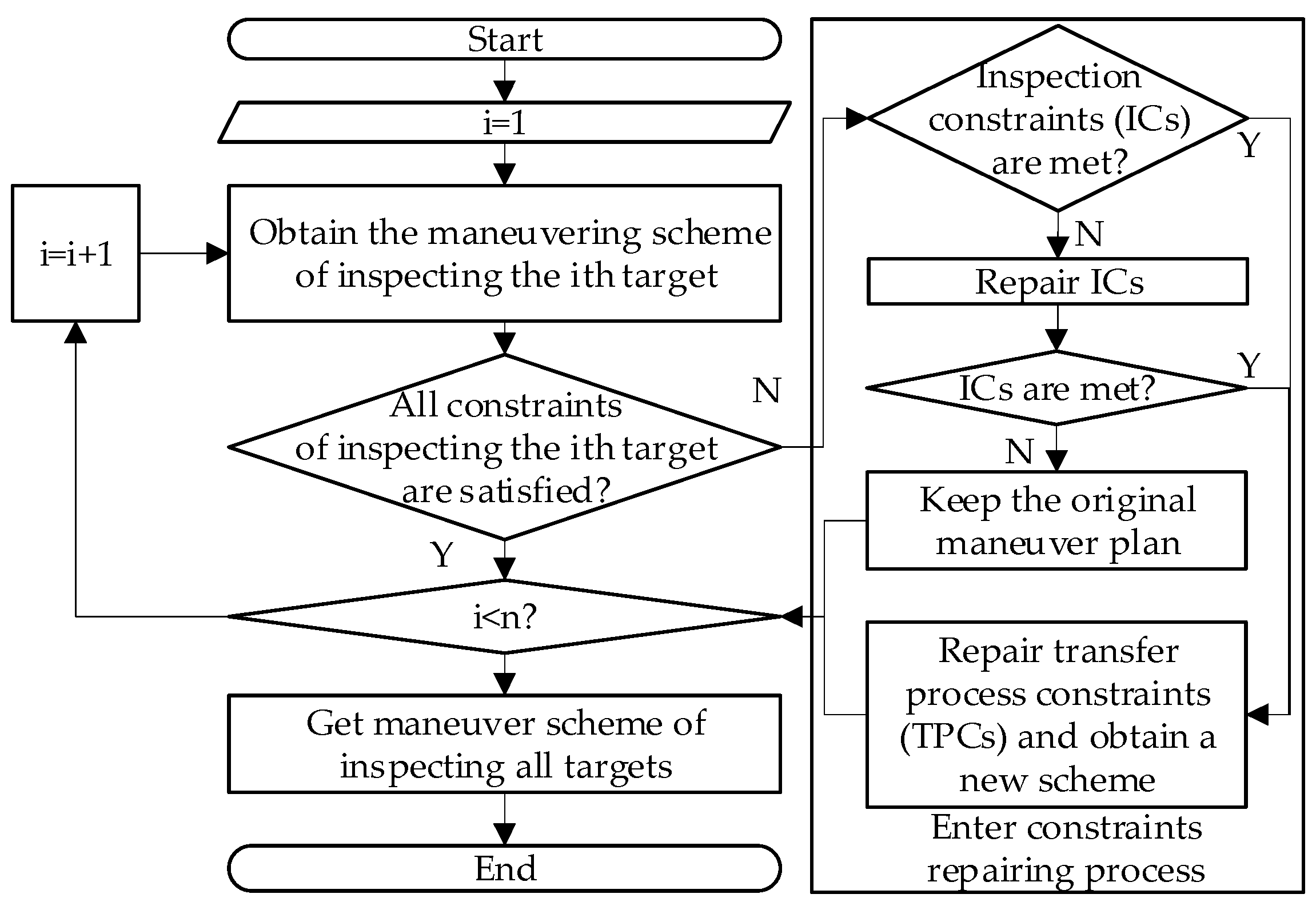
To reduce the number of penalty terms and increase the number of feasible solutions, we propose a new method based on constraint repairing, which is to enter a constraint repairing process when inspecting a satellite and the constraint is not satisfied. After the repairing process, the method can obtain a new maneuver scheme to replace the original one, and then the SS continues to inspect the next satellite according to the original design variables. The calculation process is shown in Figure 3.

Firstly, according to the original design variables, the maneuver scheme for inspecting a satellite is obtained. When the constraint conditions for inspecting the satellite are not met, the algorithm enters the repairing process to obtain a new inspection scheme. Otherwise, the original maneuver scheme is maintained and the process is repeated until all the target satellites are inspected. The calculation process of constraint repairing is as follows:

Step 1

Judge whether all constraints are met. If all constraints are met, the next target’s maneuver scheme will be calculated directly without repair until all targets have been inspected. Otherwise, go to Step 2.

Step 2

The algorithms repair the ICs first and then repair the TPCs. First, judge whether all ICs are satisfied. If satisfied, go to Step 4 to repair the TPCs. If any of the ICs are not satisfied, then go to Step 3.

Step 3

Repair the ICs, and judge whether the IC repairing is successful. If it fails, exit the calculation directly and keep the original maneuver scheme. Otherwise, continue to repair TPCs.

Step 4

Repair the TPCs and obtain a new maneuver scheme to replace the original one.

2.3.2. IC Repair Method

Firstly, we give the repair process, and then we give the repair scope satisfying the ICs.

(1)

Repair process

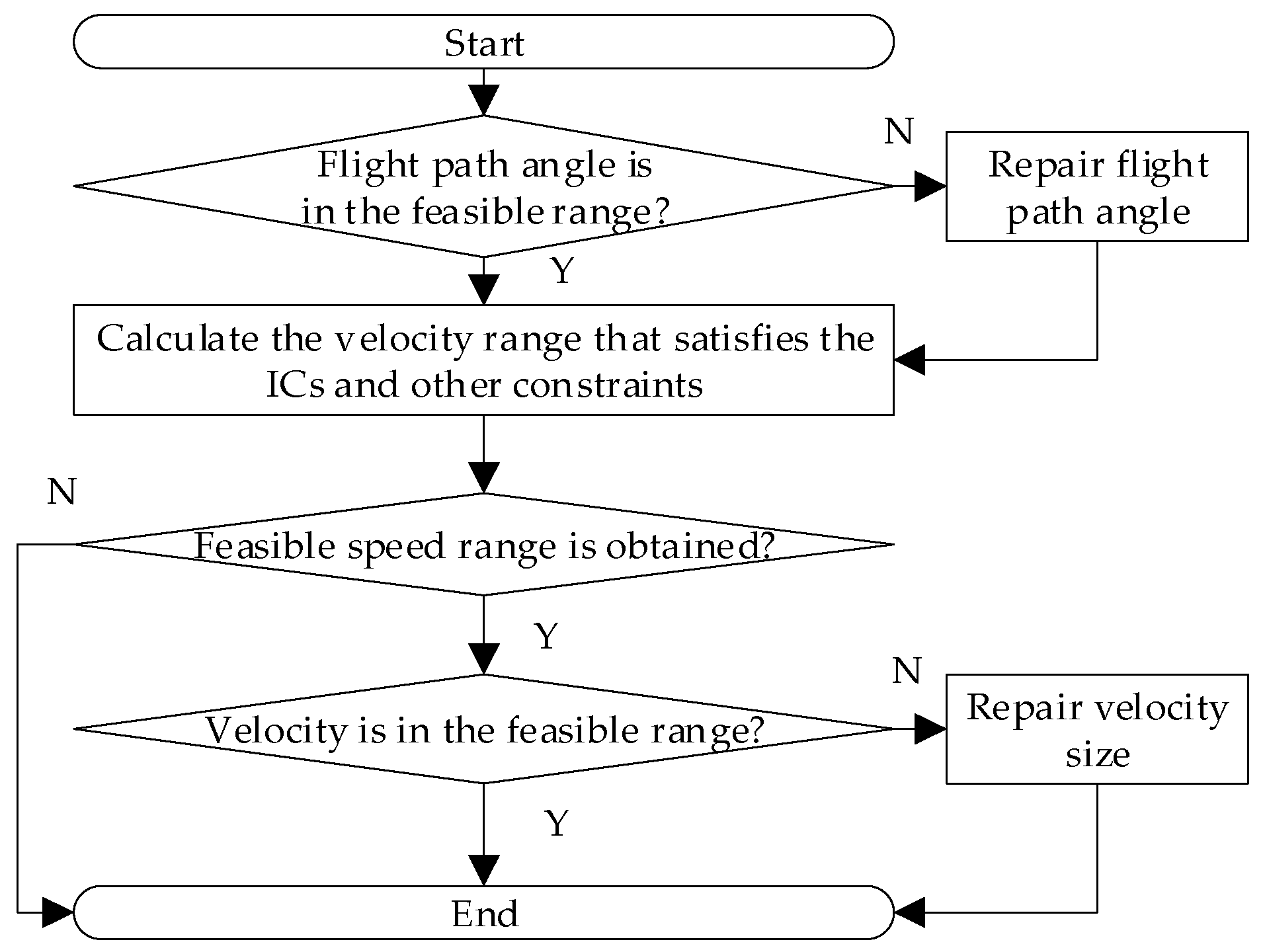
According to the expression of ASL and relative velocity constraints, the reason why the ICs are not satisfied is that the magnitude or direction of relative velocity does not meet the requirements. Because the state of the target at the terminal time is known, we can only adjust the velocity vector of the SS to meet the terminal constraints. Generally, the state of terminal flyby is represented by the flight-direction angle, also written as $\gamma$, and the velocity size, also written as $v_{\mathrm{s}}$. The flight-direction angle is defined as the angle from radius direction to velocity direction, the range of which is $0\le \gamma \le \pi$ [11].

The repair process is shown in Figure 4. First, judge whether the original terminal flight-direction angle is within the feasible range. If it is not within the feasible range, take a flight-direction angle value according to the feasible range and corresponding design variable. If it is within the feasible range, there is no need to repair it. It is necessary to provide the design variables related to the flight-direction angle. Here, the design variables corresponding to the direction of orbital maneuver are changed into the design variables of flight-direction angle.

Then, under the current flight-direction angle value, the range of flyby velocity that meets the ICs and other constraints is calculated. If there is no feasible range, withdraw the calculation because the repair is not successful. If there is a feasible range, judge whether the existing velocity is within the range. If it is, do not repair it. If it is not, judge which boundary of the feasible range the velocity size is closer to, and then repair it to the corresponding boundary value and end the calculation.

(2)

Repair scope satisfying the ICs and other constraints

Generally, the value of the flight-direction angle is given according to the design variables and the feasible range of the flight-direction angle, and the velocity range satisfying the ICs and other constraints depends on the given flight-direction angle value. By calculating the upper and lower bounds of the velocity, we can obtain the velocity according to the design variables. To sum up, given the range of flight-direction angle, we can obtain the velocity range satisfying the ICs and other constraints. The specific derivation process is shown in Appendix A.

The range of flight-direction angle is $\left\{\gamma \right|\mathbf{A}\cap \mathbf{B}\cap \mathbf{C}\}$:

$$\mathbf{A}=\{{\gamma }_{\min }\le \gamma \le {\gamma }_{\max }\}$$

(6)

$$\mathbf{B}=\{\arcsin (\sqrt{1-{e_{\max }}^2})\le \gamma \le \mathsf{\pi }-\arcsin (\sqrt{1-{e_{\max }}^2})\}$$

(7)

$$\mathbf{C}=\{\arcsin (r_{\mathrm{p}\_\min }/r)<\gamma <\mathsf{\pi }-\arcsin (r_{\mathrm{p}\_\min }/r)\}$$

(8)

where ${\gamma }_{\min }$ and ${\gamma }_{\max }$ are the lower and upper bounds of flight-direction angle, $e_{\max }$ and $r_{\mathrm{p}\_\min }$ are the maximum eccentricity and the minimum geocentric distance during the whole mission, and r is the geocentric distance of the target inspected at the time of inspection.

Given the range of the flight-direction angle, it is assumed that the value of the flight-direction angle is known according to the design variables, and the range of the velocity that satisfies the ICs and other constraints is $\left\{v_{\mathrm{s}}\right|\mathbf{D}\cap \mathbf{E}\cap \mathbf{F}\cap \mathbf{G}\cap \mathbf{H}\}$.

$$\mathbf{D}=\{v_{\min }\le v_{\mathrm{s}}\le v_{\max }\}$$

(9)

$$\mathbf{E}=\{\begin{array}{cc}\varnothing ,\hfill & \hfill {\Delta }_1<0;\\ \{(-b_1-\sqrt{{\Delta }_1})/2\le v_{\mathrm{s}}\le (-b_1+\sqrt{{\Delta }_1})/2\},\hfill & \hfill {\Delta }_1\ge 0.\end{array}$$

(10)

$${\mathbf{F}}_1=\{\begin{array}{cc}\mathbf{U},d_{\mathrm{sx}}{v}_{\mathrm{tx}}+d_{\mathrm{sy}}{v}_{\mathrm{ty}}+d_{\mathrm{sz}}{v}_{\mathrm{tz}}>0,\hfill & \hfill d_{\mathrm{sx}}\cos \gamma +d_{\mathrm{sy}}\sin \gamma =0;\\ \varnothing ,d_{\mathrm{sx}}{v}_{\mathrm{tx}}+d_{\mathrm{sy}}{v}_{\mathrm{ty}}+d_{\mathrm{sz}}{v}_{\mathrm{tz}}\le 0,\hfill & \hfill d_{\mathrm{sx}}\cos \gamma +d_{\mathrm{sy}}\sin \gamma =0;\\ v_s<\frac{d_{\mathrm{sx}}{v}_{\mathrm{tx}}+d_{\mathrm{sy}}{v}_{\mathrm{ty}}+d_{\mathrm{sz}}{v}_{\mathrm{tz}}}{d_{\mathrm{sx}}\cos \gamma +d_{\mathrm{sy}}\sin \gamma },\hfill & \hfill d_{\mathrm{sx}}\cos \gamma +d_{\mathrm{sy}}\sin \gamma >0;\\ v_s>\frac{d_{\mathrm{sx}}{v}_{\mathrm{tx}}+d_{\mathrm{sy}}{v}_{\mathrm{ty}}+d_{\mathrm{sz}}{v}_{\mathrm{tz}}}{d_{\mathrm{sx}}\cos \gamma +d_{\mathrm{sy}}\sin \gamma },\hfill & \hfill d_{\mathrm{sx}}\cos \gamma +d_{\mathrm{sy}}\sin \gamma <0;\end{array}$$

(11)

$${\mathbf{F}}_2=\{\begin{array}{cc}\mathbf{U},d_{\mathrm{sx}}{v}_{\mathrm{tx}}+d_{\mathrm{sy}}{v}_{\mathrm{ty}}+d_{\mathrm{sz}}{v}_{\mathrm{tz}}\le 0,\hfill & \hfill d_{\mathrm{sx}}\cos \gamma +d_{\mathrm{sy}}\sin \gamma =0;\\ \varnothing ,d_{\mathrm{sx}}{v}_{\mathrm{tx}}+d_{\mathrm{sy}}{v}_{\mathrm{ty}}+d_{\mathrm{sz}}{v}_{\mathrm{tz}}>0,\hfill & \hfill d_{\mathrm{sx}}\cos \gamma +d_{\mathrm{sy}}\sin \gamma =0;\\ v_s\ge \frac{d_{\mathrm{sx}}{v}_{\mathrm{tx}}+d_{\mathrm{sy}}{v}_{\mathrm{ty}}+d_{\mathrm{sz}}{v}_{\mathrm{tz}}}{d_{\mathrm{sx}}\cos \gamma +d_{\mathrm{sy}}\sin \gamma },\hfill & \hfill d_{\mathrm{sx}}\cos \gamma +d_{\mathrm{sy}}\sin \gamma >0;\\ v_s\le \frac{d_{\mathrm{sx}}{v}_{\mathrm{tx}}+d_{\mathrm{sy}}{v}_{\mathrm{ty}}+d_{\mathrm{sz}}{v}_{\mathrm{tz}}}{d_{\mathrm{sx}}\cos \gamma +d_{\mathrm{sy}}\sin \gamma },\hfill & \hfill d_{\mathrm{sx}}\cos \gamma +d_{\mathrm{sy}}\sin \gamma <0;\end{array}$$

(12)

$${\mathbf{F}}_3=\{\begin{array}{cc}\mathbf{U},\hfill & \hfill a_2=b_2=0,c_2\le 0;\\ \varnothing ,\hfill & \hfill a_2=b_2=0,c_2>0;\\ \{v_{\mathrm{s}}\le -c_2/b_2\}\hfill & \hfill a_2=0,b_2>0;\\ \{v_{\mathrm{s}}\ge -c_2/b_2\}\hfill & \hfill a_2=0,b_2<0;\\ \varnothing ,\hfill & \hfill a_2>0,{\Delta }_2<0;\\ \{(-b_2-\sqrt{{\Delta }_2})/(2a_2)\le v_{\mathrm{s}}\le (-b_2+\sqrt{{\Delta }_2})/(2a_2)\},\hfill & \hfill a_2>0,{\Delta }_2\ge 0;\\ \mathbf{U},\hfill & \hfill a_2<0,{\Delta }_2\le 0;\\ \{v_{\mathrm{s}}\le (-b_2+\sqrt{{\Delta }_2})/(2a_2)\}\cup \{v_{\mathrm{s}}\ge (-b_2-\sqrt{{\Delta }_2})/(2a_2)\},\hfill & \hfill a_2<0,{\Delta }_2>0.\end{array}$$

(13)

$$\mathbf{F}={\mathbf{F}}_1\cup ({\mathbf{F}}_2\cap {\mathbf{F}}_3)$$

(14)

$$\mathbf{G}=\{\sqrt{(-b_3-\sqrt{{\Delta }_3})/(2a_3)}\le v_{\mathrm{s}}\le \sqrt{(-b_3+\sqrt{{\Delta }_3})/(2a_3)}\}$$

(15)

$$\mathbf{H}=\{\sqrt{(-b_4-\sqrt{{\Delta }_4})/(2a_4)}\le v_{\mathrm{s}}\le \sqrt{2\mu /r}\}$$

(16)

where $a_1=1$; $b_1=-2\left({\widehat{v}}_s\cdot v_{\mathrm{t}}\right)$; $c_1={v_t}^2-\delta {v_{\max }}^2$; $a_2={\left({\widehat{d}}_{\mathrm{s}}\cdot {\widehat{v}}_s\right)}^2-{\cos }^2{\alpha }_{\min }$; $b_2=-2\left[\left({\widehat{d}}_{\mathrm{s}}\cdot {\widehat{v}}_s\right)\left({\widehat{d}}_{\mathrm{s}}\cdot v_{\mathrm{t}}\right)-{\cos }^2{\alpha }_{\min }\left({\widehat{v}}_s\cdot v_{\mathrm{t}}\right)\right]$; $c_2={\left({\widehat{d}}_{\mathrm{s}}\cdot v_{\mathrm{t}}\right)}^2-v_{\mathrm{t}}{}^2{\cos }^2{\alpha }_{\min }$; $a_3=r^2{\sin }^2(\gamma )/{\mu }^2$; $b_3=-2r{\sin }^2(\gamma )/\mu$; $c_3=1-e_{\max }{}^2$; ${\Delta }_i=b_i{}^2-4a_i{c}_i(i=1,2,3,4)$; $a_4=[r^2{\sin }^2(\gamma )-r_{\mathrm{p}\_\min }{}^2]/{\mu }^2$; $b_4=2[2r_{\mathrm{p}\_\min }{}^2-r^2{\sin }^2(\gamma )-r_{\mathrm{p}\_\min }r]/\mu r$; $c_4=4r_{\mathrm{p}\_\min }(r-r_{\mathrm{p}\_\min })/r^2$; $v_{\min }$ and $v_{\max }$ are the lower and upper limit of flyby velocity; $\mathbf{U}$ is the universal set; the projections of unit velocity vector ${\widehat{v}}_{\mathrm{s}}$, unit sun vector ${\widehat{d}}_{\mathrm{s}}$, and target terminal velocity vector $v_{\mathrm{t}}$ in the local-vertical local-horizon (LVLH) coordinate frame are $(\cos \gamma ,\sin \gamma ,0)$, $(d_{\mathrm{sx}},d_{\mathrm{sy}},d_{\mathrm{sz}})$, and $(v_{\mathrm{tx}},v_{\mathrm{ty}},v_{\mathrm{tz}})$; and $\mu$ is the gravitational parameter.

2.3.3. TPC Repair Method

After obtaining the flying velocity and direction satisfying the ICs and other constraints, it is necessary to give a complete maneuver scheme again and find the scheme satisfying the TPCs or minimizing the penalty term. If the ICs are satisfied but the TPCs are not satisfied at the beginning, we can also use this method to obtain a complete maneuver scheme.

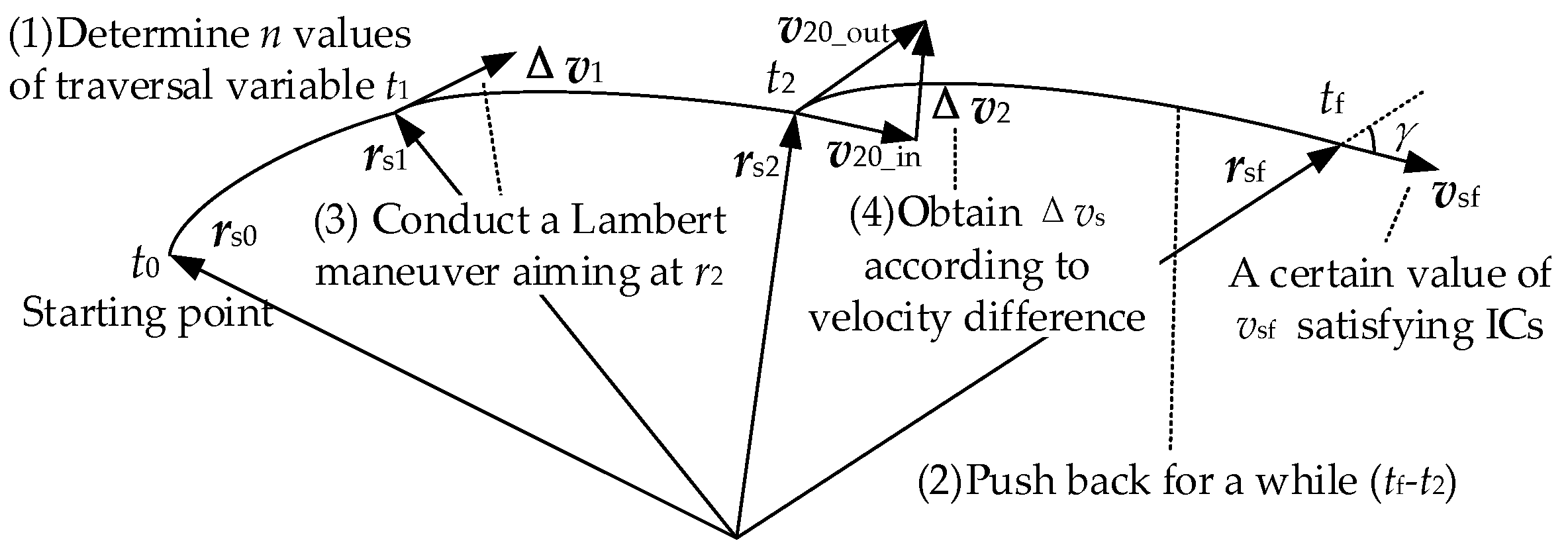
Now, the velocity direction and size of the terminal flyby are known. Once given the time of two pulses maneuver, we can obtain the components of two pulses.

Firstly, as shown in Equation (17), we need to determine n values of traversal variable t₁.

$$t_1=t_{1\_\mathrm{l}}+i\times (t_{1\_\mathrm{u}}-t_{1\_\mathrm{l}})/(n-1)$$

(17)

where $0\le i\le n-1,i\in N$, $t_{1\_\mathrm{l}}$ and $t_{1\_\mathrm{u}}$ are the lower and upper bounds of the variable $t_1$, respectively, and n is the number of traversal calculations.

Secondly, t₂ is the end time of the mission minus a fixed value, that is, pushing backward for a fixed period of time, and then the position state of the second maneuver is obtained.

Thirdly, traversing the variable time t₁ and aiming at the second maneuver position, the SS applies a Lambert maneuver at the corresponding first maneuver position.

Finally, when reaching the second maneuver position, we can obtain the velocity component of the second maneuver by subtracting the actual velocity from the desired aiming velocity.

After traversing all time t₁, the one with the smallest augmented objective function is selected as the actual inspection scheme. The whole process is shown in Figure 5.

3. Example Analysis

Two examples of MSFI are calculated to test the optimization effect of the proposed algorithm. The first test case involves a relatively diverse set of targets, and the second one involves a more clustered set of targets.

3.1. Example 1

3.1.1. Example Configuration

The first test case involves a relatively diverse set of targets. They are selected from current STARLINK satellites, which will be potential customers for such an inspection service. The SS and target satellites are shown in

Table 1. SS and target satellite orbit parameters of example 1.

Num.	Name	a/km	e	i/°	Ω/°	ω/°	θ/°	u/°
/	SS	6928.14	0.00	40.00	0.43	0.00	0.00	0.00
1	STARLINK-2158	6929.58	0.00	53.18	73.31	75.61	309.16	24.77
2	STARLINK-1532	6931.72	0.00	53.01	328.37	53.56	308.63	2.19
3	STARLINK-1230	6931.73	0.00	52.95	278.29	47.61	309.61	357.22
4	STARLINK-2201	6932.90	0.00	97.38	297.28	63.06	178.89	241.95
5	STARLINK-3005	6884.30	0.00	97.54	7.08	297.02	162.86	99.88
6	STARLINK-2574	6926.66	0.00	52.99	213.21	77.02	143.12	220.14
7	STARLINK-1308	6931.75	0.00	53.15	38.35	51.92	305.32	357.24
8	STARLINK-1084	6929.18	0.00	52.99	218.23	73.63	313.84	27.47
9	STARLINK-2206	6905.42	0.00	97.38	299.46	103.13	96.39	199.52

. The starting time of the mission is 04:00:00 on 27 August 2021 (UTCG). The data are from “STARLINK TLEs” on the website [32], which are current as of 27 August 2021 02:00:56 UTC (Day 239).

The minimum and maximum times of a single inspection mission are 2 and 24 h, respectively. The specific impulse of the engine is about 290.82 s, and the initial mass is 2000 kg. The lower limit of ASL is 50°, and the maximum relative velocity is 10.5 km/s. The upper limit of a single maneuver is 1000 m/s, and the lower limit of the perigee height is 200 km. The lower bound of the first maneuver time is the initial slide time (IST), and the upper bound is the single inspection mission time (SIMT) minus the end slide time (EST) and the minimum spacing between thruster impulses (MSTI). The lower bound of the second maneuver time is the first maneuver time plus MSTI, and the upper bound is the SIMT minus EST. We set IST = EST = MSTI = 300 s.

In the optimization model based on constraint repairing, the upper and lower bounds of the flyby flight-direction angle are 75–105°, and the upper and lower bounds of the flyby velocity are 0–11.2 km/s. The maximum eccentricity is set to 0.7. The lower bound of the first maneuver time is the IST, and the upper bound is the minimum value of T₁ and T₂. T₁ is the IST plus the first revolution flight time of SS. T₂ is the SIMT minus the EST and MSTI. The number of traversal calculations is 89, and the second maneuver is executed 300 s before the end of each transfer.

The parameters of the HEGA are as follows: The population size is 600. The evolution generation is 700. These two parameters are chosen because the optimization results are best in these two values after many trials. The mutation probability of integer and real variables is 0.7, and the crossover probability is 0.8. The reason why the mutation and crossover probability are so large is that the HEGA uses the elite strategy, which may cause a premature problem if the probability of mutation and crossover is too small. The number of individuals in the tournament is 3. The penalty factors of penalty function are as follows: The penalty factors of maneuver velocity, perigee height, ASL, and flyby relative velocity are 10⁶, 10⁵, 10⁷, and 10⁴, respectively. The units of all parameters are international standard units.

3.1.2. Simulation Results and Method Comparison

To compare and analyze the optimization effect of the method proposed in this paper, the nonrepair method is used for optimization calculation. The nonrepair method is the optimization method without any constraint repair and only relies on the penalty function method for optimization.

In all calculations, the computer configuration used is Intel (R) Xeon (R) E5-2690 V4 (2.6 GHz, 64 GB). Because of the randomness of the HEGA, we carry out 20 independent calculations using the constraint repairing method and the nonrepair method and give the best solution in

Table 2. Population size, evolutionary generation, velocity increment, fuel consumption, computation time, and mission time for two methods.

Method	Population Size	Evolution Generation	Velocity Increment (m/s)	Fuel Consumption (kg)	Computation Time (min)	Mission Time (h)
Nonrepair method	2000	2000	667.57	417.65	444.59	118.30
Constraint repairing method	600	700	1164.83	670.99	222.50	130.53

, which contains the population size, evolution generation, velocity increment, fuel consumption, computation time, and mission time.

Compared with the nonrepair method, the constraint repairing method cannot obtain a better solution, but it can also obtain a reasonable solution in a short time. We give the constraints of the best solution scheme for the nonrepair method, which is shown in

Table 3. Constraint values of each inspection task of example 1.

Target Sequence	ASL (°)	Relative Velocity (km/s)
2	87.29	3.46
3	112.09	7.37
8	117.83	10.46
6	115.50	10.50
5	109.38	7.32
9	71.94	9.54
4	70.63	9.69
1	63.36	6.72
7	68.81	3.95
Constraint boundary	50.00	10.50

. As we can see, the constraints are easy to meet, and the constraint repairing method might not suit this problem-solving. Therefore, we make a more clustered case in example 2, whose constraints are more difficult to satisfy.

3.2. Example 2

3.2.1. Example Configuration

The second test case involves a more clustered set of targets. The specific parameters of the SS and target satellites are shown in

Table 4. SS and target satellite orbit parameters of example 2.

Name	a/km	e	i/°	Ω/°	ω/°	θ/°	u/°
SS	7078.14	0.00	98.19	50.97	0.00	0.00	0.00
Target satellite 1	6927.00	0.00	97.00	140.00	127.00	280.00	47.00
Target satellite 2	6999.00	0.00	97.00	139.00	117.00	202.00	319.00
Target satellite 3	6999.00	0.00	97.00	139.00	62.00	77.00	139.00
Target satellite 4	6996.00	0.00	97.00	139.00	60.00	169.00	229.00
Target satellite 5	6990.00	0.00	97.00	139.00	197.00	234.00	71.00
Target satellite 6	6986.00	0.00	98.00	83.00	116.00	43.00	159.00
Target satellite 7	6807.00	0.00	97.00	84.00	111.00	171.00	282.00
Target satellite 8	6936.00	0.00	98.00	139.00	228.00	49.00	277.00
Target satellite 9	6958.00	0.00	98.00	62.00	78.00	17.00	95.00

. There are nine targets, which are distributed in a sun-synchronous orbit. The starting time of the mission is 20:00:00 on 31 July 2021 (UTCG), and other parameters are the same as the configuration of example 1. Firstly, the simulation results of optimization are given, then the effects of various constraints on the results are given, and finally, the comparison results of two different methods are given.

3.2.2. Simulation Results and Constraint Analysis

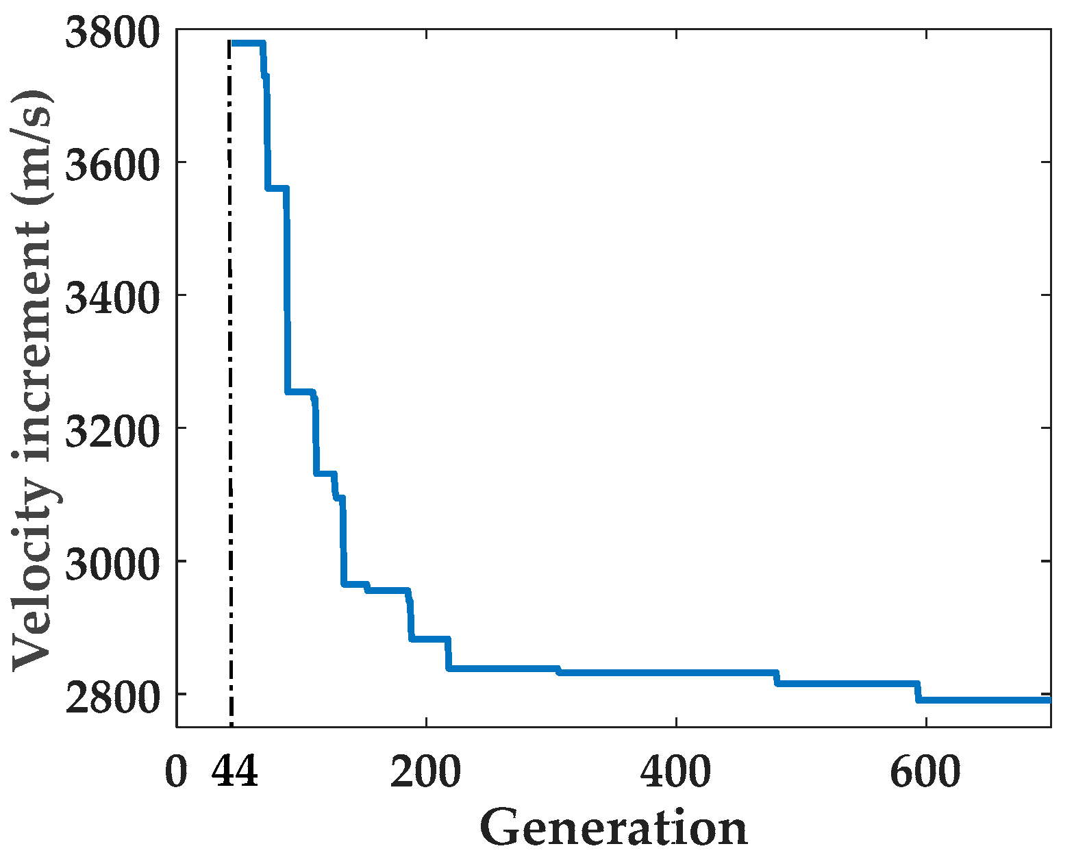
Due to the randomness of the HEGA, we carry out 20 independent calculations, in which the optimal velocity increment is 2668.60 m/s (the propellant consumption is 1215.89 kg), the mission time is 61.29 h, and the optimal inspection sequence is {2,4,1,3,5,8,9,6,7}. The specific maneuver scheme is shown in

Table 5. Orbit maneuver scheme.

Maneuver Sequence	Time (h)	J2000 Impulse (m/s)	Velocity Increment (m/s)
1-1	0.24	(1.90, 3.17, −3.57)	5.14
1-2	2.32	(−87.95, −117.21, 38.11)	151.42
2-1	8.93	(−0.62, −1.08, 1.39)	1.87
2-2	9.03	(−19.41, −23.18, −3.31)	30.41
3-1	20.07	(−6.19, −1.95, −24.87)	25.70
3-2	30.42	(92.33, 130.43, −72.31)	175.40
4-1	30.60	(−6.63, −7.87, −1.35)	10.38
4-2	30.68	(−70.68, −64.61, −98.75)	137.56
5-1	33.91	(−0.01, −0.01, −0.03)	0.03
5-2	34.00	(−12.09, −17.44, 11.05)	23.92
6-1	46.07	(−4.78, −5.62, −1.23)	7.48
6-2	46.15	(−28.20, −12.26, −98.54)	103.23
7-1	48.85	(−305.33, −321.12, −242.88)	505.31
7-2	52.85	(0.20, −3.08, 14.55)	14.87
8-1	53.02	(−441.61, −486.05, −256.80)	705.13
8-2	56.12	(−392.92, −423.15, −269.24)	637.13
9-1	57.71	(−13.22, −18.82, 10.98)	25.48
9-2	61.21	(−68.00, −75.35, −37.32)	108.14

. The optimal evolution curve is given. As shown in Figure 6, the feasible solution is obtained in the 44th generation of evolution. Through continuous evolution, the final result is obtained.

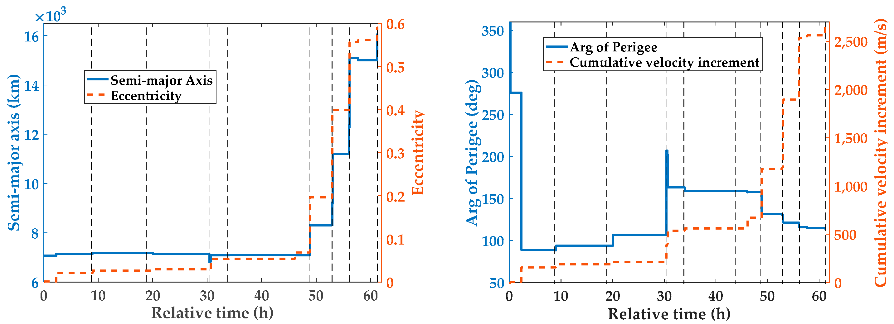
The time-varying processes of the semimajor axis, eccentricity, argument of perigee (AOP), and cumulative velocity increment of the SS are given, as shown in Figure 7. The vertical lines in the figure represent the inspection time of nine different targets. It can be seen that the semimajor axis and eccentricity of the SS increase gradually, and the greater the change of the two, the greater the velocity increment. The AOP almost remains in the range of 100–150°, which will reduce the fuel consumption in the aspects of changing AOP.

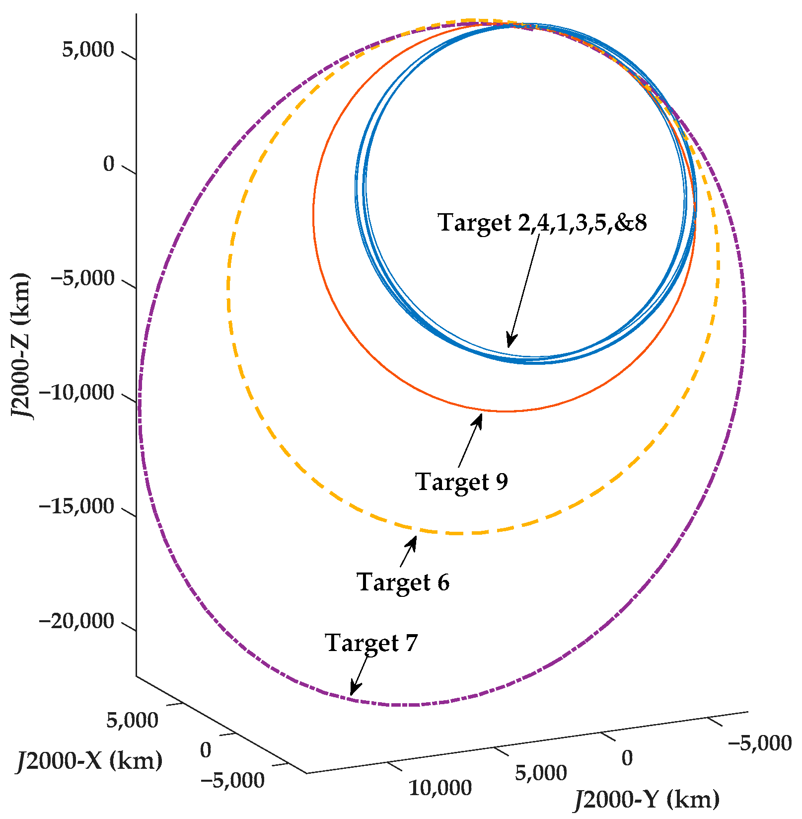
As shown in Figure 8, the trajectories of the SS are given. Different trajectories represent the trajectories of inspecting different targets. Combined with Figure 7, it can be seen that the semimajor axis and eccentricity of the SS are increasing, but the apsidal line is kept near a region and remains unchanged in the later stage. This kind of phenomenon is an expression of saving propellant.

As shown in

Table 6. Constraint values of each inspection task of example 2.

Target Sequence	ASL (°)	Relative Velocity (km/s)
2	52.51	10.45
4	52.22	10.47
1	51.80	10.50
3	51.89	10.43
5	51.56	10.44
8	51.35	10.49
9	50.00	1.82
6	50.00	5.12
7	50.00	5.36
Constraint boundary	50.00	10.50

, the constraint values for completing each inspection task are given. Most of the ASLs are close to the lower limit of the constraint, three of which even are taken to 50.00°. Relative velocity constraints are also basically around 10.5 km/s. They all prove that the constraints proposed in this problem are difficult to satisfy.

To analyze the influence of different constraints on the results, we give the optimal inspection schemes without considering ASL and relative velocity constraints.

Firstly, ASL constraints are not considered. In this example, the minimum ASL is set to 0°. The optimal inspection sequence, velocity increment, propellant consumption, and mission time are shown in

Table 7. The results of minimum velocity increment under different constraints.

Constraint Considerations	Velocity Increment (m/s)	Fuel Consumption (kg)	Mission Time (h)	Inspection Order
All constraints	2668.60	1215.89	61.29	{2,4,1,3,5,8,9,6,7}
Without ASL constraints	676.85	422.79	126.50	{8,2,4,1,6,5,9,3,7}
Without relative velocity constraints	2379.45	1132.16	39.56	{8,9,4,1,3,5,2,6,7}

. The velocity increment is greatly reduced compared with the case in which all constraints are considered, proving that ASL constraints have a great impact on the optimal inspection scheme.

Then, the relative velocity constraints are not considered. In this example, the maximum relative velocity is set to positive infinity. Similarly, the result is shown in Table 7. The consumption of propellant has slightly decreased, but the inspection sequence has changed a lot. Without considering the constraints, the number of feasible solutions will increase, and more combinations of feasible inspection sequences will be produced so that different sequences can also obtain better propellant consumption results.

3.2.3. Comparison with the Nonrepair Method

Similarly, to compare the calculation effect of the two different methods in this example, we change the number of satellites to three, six, and nine and compare the results of the two methods under different numbers of satellites. Each example is calculated 20 times, and the best one is taken as the final result. The population size and evolution generation settings are shown in

Table 8. Population size, evolutionary generation, velocity increment, fuel consumption, computation time, and mission time for different numbers of targets and different methods.

Target Sets	Method	Population Size	Evolution Generation	Velocity Increment (m/s)	Fuel Consumption (kg)	Computation Time (min)	Mission Time (h)
{1, 2, 3}	Nonrepair method	1000	1000	152.42	104.15	46.49	60.79
	Constraint repairing method	300	400	170.50	116.14	26.07	42.71
{1, 2, …, 6}	Nonrepair method	1500	1500	2533.09	1177.70	196.96	65.88
	Constraint repairing method	500	500	2526.77	1175.88	85.44	31.99
{1, 2, …, 9}	Nonrepair method	2000	2000	2677.08	1218.22	531.52	104.76
	Constraint repairing method	600	700	2668.60	1215.89	203.47	61.29

. The optimal velocity increment, propellant consumption, mission time, and calculation time obtained by different methods under different numbers of satellites are also shown in Table 8.

Generally, the more satellites there are, the more difficult it is to satisfy the constraints. When the number of satellites is three, the velocity increment obtained by the nonrepair optimization method is relatively low, and the results obtained by the constrained repair optimization method in a short time are close to the optimal solution, but the optimization effect is still not good enough. When the number of satellites increases to six, the optimal velocity increment is the result of the constraint repairing method, and the calculation time is at least half of the nonrepair method. When the number of satellites increases to nine, the conclusion is similar.

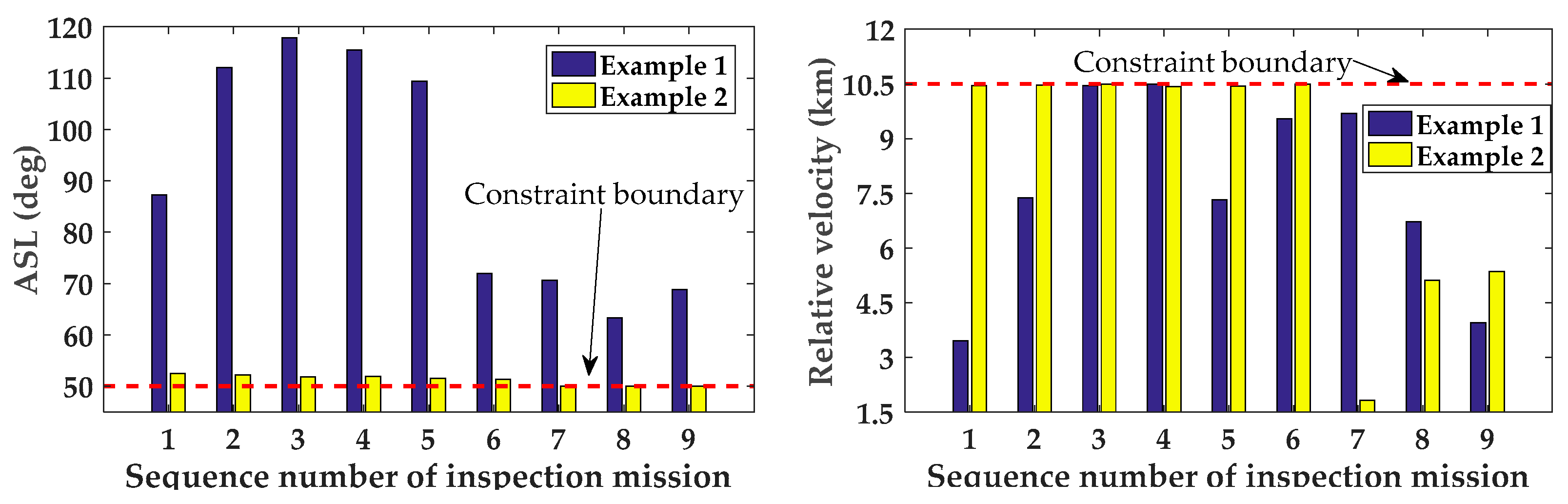
In Figure 9, we compare the ASL and relative velocity constraints of two examples, which gives the value of the constraint in different inspection missions. Compared with example 1, most of the ASL and relative velocity constraints for example 2 are near the bound value. Therefore, example 2 is a case whose constraints are difficult to satisfy, which may be more suitable for using the constraint repairing method.

From examples 1 and 2, we can make conclusions as follows: When the constraints are easy to meet, the nonrepair optimization method can quickly find feasible solutions and quickly optimize, which has obvious advantages. However, the constraint repairing optimization method can also obtain a reasonable result in a short time. When the constraints are hard to meet, it is easy to find a feasible solution by using the constraint repairing method, and it can also obtain better results in a short time, which is more suitable for solving such problems.

4. Conclusions

In this paper, we propose a trajectory optimization method of MSFI based on constraint repairing. Firstly, we give the mission flow based on coplanar maneuver, and then we define the trajectory optimization model from the design variables, constraints, and objective function. Finally, we propose the trajectory optimization method based on constraint repairing from three aspects: the algorithm framework, the IC repair method, and the TPC repair method. Compared with the nonrepair method, through the calculation of the two different examples, the conclusion is as follows: When the constraints are easy to meet, the constraint repairing optimization method can obtain a reasonable solution in a short time. When the constraints are hard to meet, the optimization method based on constraint repairing is not only slightly better than the nonrepair method in optimization effect but also more than twice better than the nonrepair method in optimization efficiency, which is more suitable for solving this kind of problem.

In future research, it is necessary to consider the problem of multiple SSs inspecting multiple targets, that is, the M2M MSFI problem, which also needs an efficient algorithm combined with task allocation variables.

References

- Li, W.-J.; Cheng, D.-Y.; Liu, X.-G.; Wang, Y.-B.; Shi, W.-H.; Tang, Z.-X.; Gao, F.; Zeng, F.-M.; Chai, H.-Y.; Luo, W.-B.; et al. On-Orbit Service (OOS) of Spacecraft: A Review of Engineering Developments. Prog. Aerosp. Sci. 2019, 108, 32–120. [Google Scholar] [CrossRef]
- Qiu, L.; Tang, L.; Zhong, R. Toward the Recognition of Spacecraft Feature Components: A New Benchmark and a New Model. Astrodynamics 2021. [Google Scholar] [CrossRef]
- Zhang, G.; Mortari, D.; Zhou, D. Constrained Multiple-Revolution Lambert’s Problem. J. Guid. Control Dyn. 2010, 33, 1779–1786. [Google Scholar] [CrossRef]
- Huang, Y.; Pan, B.; Tang, S. Constrained Multiple-Revolution Lambert Problem with Transverse-Eccentricity-Based Method. J. Northwest Univ. (Nat. Sci. Ed.) 2014, 44, 23–30. [Google Scholar]
- Thompson, B.F.; Rostowfske, L.J. Practical Constraints for the Applied Lambert Problem. J. Guid. Control Dyn. 2020, 43, 967–974. [Google Scholar] [CrossRef]
- Luo, Q.; Meng, Z.; Han, C. Solution Algorithm of a Quasi-Lambert’s Problem with Fixed Flight-Direction Angle Constraint. Celest. Mech. Dyn. Astr. 2011, 109, 409–427. [Google Scholar] [CrossRef]
- Karthikeyan, K.; Joshi, A. Solution of Lambert’s Theorem with Additional Terminal Constraints. In Proceedings of the AIAA Atmospheric Flight Mechanics Conference, Atlanta, GA, USA, 16–20 June 2014. [Google Scholar]
- Shirazia, A.; Ceberiob, J.; Lozanoa, J.A. An Evolutionary Discretized Lambert Approach for Optimal Long-range Rendezvous Considering Impulse Limit. Aerosp. Sci. Technol. 2019, 94, 105400. [Google Scholar] [CrossRef] [Green Version]
- Thompson, B.F.; Choi, K.K.; Piggott, S.W.; Beaver, S.R. Orbital Targeting Based on Hodograph Theory for Improved Rendezvous Safety. J. Guid. Control Dyn. 2010, 33, 1566–1576. [Google Scholar] [CrossRef]
- Taur, D.-R.; Coverstone-Carroll, V.; Prussing, J.E. Optimal Impulsive Time-Fixed Orbital Rendezvous and Interception with Path Constraints. J. Guid. Control Dyn. 1995, 18, 54–60. [Google Scholar] [CrossRef]
- Zhang, G.; Zhou, D.; Mortari, D.; Henderson, T.A. Analytical Study of Tangent Orbit and Conditions for Its Solution Existence. J. Guid. Control Dyn. 2012, 35, 186–194. [Google Scholar] [CrossRef]
- Zhang, J.; Luo, Y.; Tang, G. Effects of In-track Maneuver on Sun Illumination Conditions of Near-circular Low Earth orbits. Adv. Space Res. 2014, 53, 509–517. [Google Scholar] [CrossRef]
- Zhang, J.; Li, H.; Luo, Y.; Tang, G. Effects of In-Track Maneuver on the Ground Track of Near-Circular Orbits. J. Guid. Control Dyn. 2015, 37, 1373–1378. [Google Scholar] [CrossRef]
- Liu, J.; Shan, J.; Liu, Q. Optimal Pulsed Guidance Law with Terminal Impact Angle Constraint. P. I. Mech. Eng. G-J. Aer. 2017, 231, 1993–2005. [Google Scholar] [CrossRef]
- Xie, L.; Zhang, Y.; Xu, J. Optimal Two-Impulse Space Interception with Multiple Constraints. Front. Inf. Technol. Electron. Eng. 2020, 21, 1085–1107. [Google Scholar] [CrossRef]
- Hudson, J.S.; Kolosa, D. Versatile On-Orbit Servicing Mission Design in Geosynchronous Earth Orbit. J. Spacecr. Rocket. 2020, 57, 844–850. [Google Scholar] [CrossRef]
- Zhang, J.; Luo, Y.; Tang, G. Hybrid Planning for LEO Long-Duration Multi-Spacecraft Rendezvous Mission. Sci. China Technol. Sci. 2012, 55, 233–243. [Google Scholar] [CrossRef]
- Zhao, S.; Zhang, J.; Xiang, K.; Qi, R. Target Sequence Optimization for Multiple Debris Rendezvous Using Low Thrust Based on Characteristics of SSO. Astrodynamics 2017, 1, 85–99. [Google Scholar] [CrossRef]
- Barea, A.; Urrutxua, H.; Cadarso, L. Large-Scale Object Selection and Trajectory Planning for Multi-Target Space Debris Removal Missions. ACTA Astronaut. 2020, 170, 289–301. [Google Scholar] [CrossRef]
- Li, C.; Xu, B. Optimal Scheduling of Multiple Sun-Synchronous Orbit Satellites Refueling. Adv. Space Res. 2020, 66, 345–358. [Google Scholar] [CrossRef]
- Zhang, T.-J.; Yang, Y.-K.; Wang, B.-H.; Li, Z.; Shen, H.-X.; Li, H.-N. Optimal Scheduling for Location Geosynchronous Satellites Refueling Problem. ACTA Astronaut. 2019, 163, 264–271. [Google Scholar] [CrossRef]
- Zhu, X.; Zhang, C.; Sun, R.; Chen, J.; Wan, X. Orbit Determination for Fuel Station in Multiple SSO Spacecraft Refueling Considering the J2 Perturbation. Aerosp. Sci. Technol. 2020, 105, 105994. [Google Scholar] [CrossRef]
- Guo, S.; Zhou, W.; Zhang, J.; Sun, F.; Yu, D. Integrated Constellation Design and Deployment Method for a Regional Augmented Navigation Satellite System Using Piggyback Launches. Astrodynamics 2021, 5, 49–60. [Google Scholar] [CrossRef]
- Yu, J.; Chen, X.; Chen, L. Orbital Rendezvous Mission Planning with Complex Constraints. P. I. Mech. Eng. G-J. Aer. 2016, 230, 296–306. [Google Scholar] [CrossRef]
- Du, B.; Zhao, Y.; Chen, L.; Yao, W. Mission Programming of Peer-to-Peer Refueling on Non-Coplanar Circular Orbit. Chin. Space Sci. Technol. 2015, 35, 58–65. [Google Scholar]
- Zhang, J.; Wu, M. Necessary and Sufficient Conditions of the Rendezvous between a Single Spacecraft and Three Non-Coplanar Walker Constellation Satellites. Sci. China Technol. Sci. 2011, 54, 2254–2262. [Google Scholar] [CrossRef]
- Zhou, Y.; Yan, Y.; Huang, X.; Yang, Y.; Zhang, H. Mission Planning Optimization for the Visual Inspection of Multiple Geosynchronous Satellites. Eng. Optim. 2015, 47, 1543–1563. [Google Scholar] [CrossRef]
- Zhu, Z.; Yan, Y. Two-Tangent-Impulse Flyby of Space Target from an Elliptic Initial Orbit. Adv. Space Res. 2016, 57, 2177–2186. [Google Scholar] [CrossRef]
- Zhao, Z. Planning Approaches for Multi-Spacecraft On-Orbit Service Missions. Master’s Thesis, National University of Defense Technology, Changsha, China, November 2016. [Google Scholar]
- Ma, N. Fuel Optimal Orbit Design of Satellite Constellation Traversal Using Finite Thrust Mode. Master’s Thesis, Harbin Institute of Technology, Harbin, China, June 2017. [Google Scholar]
- Peng, C.; Zhang, J.; Yan, B.; Zhou, H.; Luo, Y. Multi-Satellite Responsive Inspection Mission Planning with Multiple Constraints. Chin. Space Sci. Technol. 2021, in press. [Google Scholar]
- CelesTrak: Current Supplemental Two-Line Element Sets. Available online: http://celestrak.com/NORAD/elements/supplemental/ (accessed on 27 August 2021).
Figure 1.
Task flow of multisatellite flyby inspection.
Figure 2.
ASL constraints diagram.
Figure 3.
Calculation flow chart based on constraint repairing.
Figure 4.
Flow chart of repairing ICs.
Figure 5.
Schematic diagram of TPC repair process.
Figure 6.
Evolution history of optimal solution.
Figure 7.
Time-dependent curves of orbit parameters and velocity increment of SS.
Figure 8.
Optimal trajectory.
Figure 9.
Comparison of constraints for two different examples.