
A New 3D Shaping Method for Low-Thrust Trajectories between Non-Intersect Orbits


1
School of Aerospace Engineering, Tsinghua University, Beijing 100084, China
2
Beijing Institute of Aerospace Systems Engineering, Beijing 100076, China
*
Author to whom correspondence should be addressed.
Aerospace 2021, 8(11), 315; https://0-doi-org.brum.beds.ac.uk/10.3390/aerospace8110315
Submission received: 1 September 2021
/
Revised: 8 October 2021
/
Accepted: 11 October 2021
/
Published: 24 October 2021
(This article belongs to the Special Issue Spacecraft Dynamics and Control)
Abstract
:This paper proposes a new shape-based method in spherical coordinates to solve three-dimensional rendezvous problems. Compared with the existing shape-based methods, the proposed method does not need parameter optimization. Moreover, it improves the flexibility of orbit fitting, greatly reduces the velocity increment and maximum thrust acceleration, and ensures the orbit safety to a certain extent. The shaping function can provide the initial estimate for numerical trajectory optimization and improve the convergence rate in a certain range when combined with the normalization method. The superiority of the proposed method over the existing methods is demonstrated by two numerical examples. Its effectiveness at initial estimation generation in the indirect optimization of a low-thrust trajectory is demonstrated by the third example.
1. Introduction
The continuous low-thrust propulsion system has attracted great attention because of its higher specific impulse and consequently less fuel consumption compared with impulsive propulsion systems. There are three main categories of optimization methods to optimize the low-thrust trajectory: the direct methods [1,2,3], indirect methods [3,4,5,6], and hybrid methods [7,8,9]. For the gradient-based versions of these methods, a good initial value estimate is key to improving the convergence of optimization. To provide the initial guesses, especially for a general three-dimensional (3D) rendezvous problem, the shape-based method can be used to approximate the near-optimal trajectory through shaping function design. In particular, when the shape is used as a nominal trajectory and then combined with the indirect method, it can greatly improve the computational efficiency [10].
At present, the shape-based methods can be divided into two categories according to whether their shape functions consist of free optimization parameters: one has no parameter optimization, and the other has to resort to the help from parameter optimization. The former has obvious advantages in terms of computational speed and efficiency. Petropoulos and Longuski [11] proposed the first shape-based method without optimization, which uses an exponential sinusoid to describe a coplanar trajectory. It is simple in form but cannot meet the boundary conditions of position and velocity at the same time, so it cannot solve rendezvous problems. Then, the inverse polynomial method was introduced by Wall and Conway [12]. This has enough coefficients to satisfy the in-plane boundary conditions. Because of its limited number of extrema, it cannot solve multirevolution problems. Accordingly, Wall and Pols [13] used the cosine inverse polynomial (cosine IP) to design the coplanar trajectory. In order to solve the problem of 3D transfer and rendezvous problems, Wall [14] and Novak [15] both designed the out-of-plane component; however, this only performs well when the elevation angle is small. Later, Xie [16,17] and Zeng [18] proposed methods that are suitable for transfer and rendezvous problems with any elevation angle, respectively. The difference between these two methods is that Xie’s method [17] designs the in-plane and out-of-plane shapes separately and selects the polynomial as the shaping function, while Zeng’s method [18] does not design the shape separately in three dimensions and uses a Fourier series as the shaping function. Both of these approaches can provide solutions for transfer and rendezvous problems with large elevation angles. However, the velocity increment and maximum thrust acceleration of the two methods are much larger than those of the 3D inverse polynomial method, which makes the trajectory designed by these two methods far from the optimal trajectory.
There are two main contributions of this paper. Firstly, a new shape-based 3D method is proposed for rendezvous problems, which considers the advantages of Novak’s method [15] and Zeng’s method [18] in the design and improves some deficiencies existing in these two methods. It widens the application scope of the shape-based method and reduces the fuel consumption. The proposed method satisfies the boundary conditions and the equation of motion constraints and does not require parameter optimization. It is able to effectively reduce the velocity increment and maximum thrust acceleration and provide good initial guesses for the local optimization of low-thrust trajectories. Secondly, adjoint normalization [19] is added into the process of combining the shape-based method with the indirect method, which greatly improves the convergence rate.
This paper is organized as follows. In Section 2, a new shape-based method is proposed. Firstly, the dynamic model of a spacecraft and the 3D trajectory models in spherical coordinates are given, and then the shaping functions are determined. Section 3 introduces the method of applying adjoint normalization into the process of combining the shape-based method with the indirect method in cylindrical coordinates. The specific examples of rendezvous problems and the shape-based method in combination with optimization problems are described in Section 4. Finally, the conclusion is deduced in Section 5.
2. Shape-Based Method for 3D Orbital Rendezvous
In this section, a shape-based method that approximates the low-thrust trajectory with the shaping functions parameterized in the spherical coordinate frame is introduced for the three-dimensional (3D) orbital rendezvous. The boundary conditions and dynamical constraints of the rendezvous are automatically satisfied by developing a new shape-based approach based on the cosine IP method [13] and Zeng’s method [18] empirically to reduce fuel consumption.
2.1. Low-Thrust Dynamics and Shape Design in Spherical Coordinates
The spacecraft in an interplanetary rendezvous is subject to the central gravitational force of the Sun and propelled by a low-thrust propulsion system. For the 3D trajectory design, the corresponding dynamics are given [17] as follows:
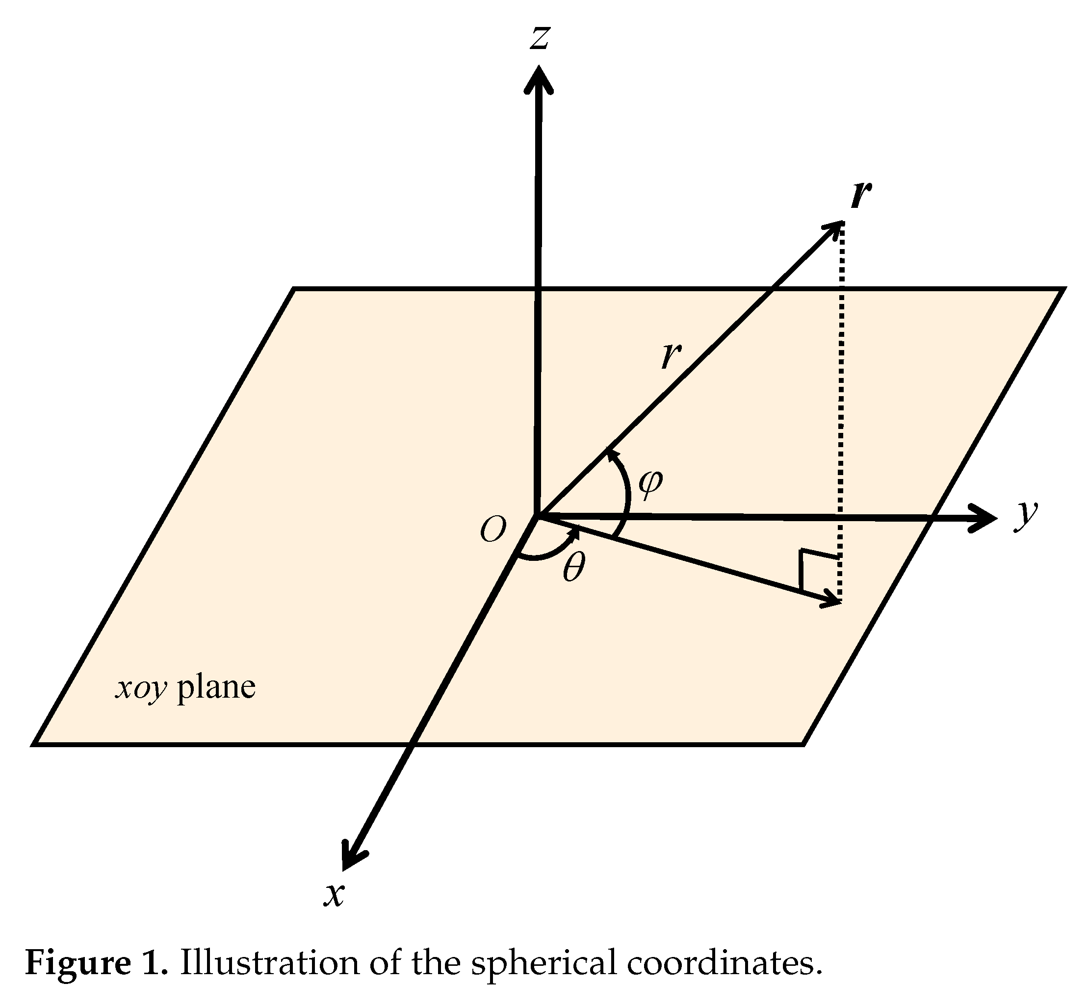
where is the position vector of a spacecraft with in the spherical inertial frame, is the low-thrust acceleration, and is the gravitational parameter of the Sun. The spherical coordinate frame is defined as Figure 1, where r is the distance from the Sun to the spacecraft, is the azimuthal angle, and is the elevation angle. Equation (1) can also be written as
where and denote the derivative and double derivative with respect to , respectively. The trajectory parameterized with will be given by the shaping functions, and the low-thrust acceleration can then be obtained by Equation (2) to approximate the rendezvous.
The shape designed by Novak [15] empirically has a smaller and in most coplanar transfer and rendezvous cases compared with other methods. However, for the cases with a large elevation angle , it may lead to or and thus cannot obtain a reasonable trajectory. Inspired by the shaping functions proposed in [18], an improved interpolation between the initial and target orbits is proposed here to design the elevation angle . Combined with the designed in [15] by introducing a mid-plane, the proposed shape can broaden the application range to the 3D rendezvous trajectory with a large elevation angle and reduce the velocity increment and maximum low-thrust acceleration to a certain extent empirically.
2.1.1. Shaping the Elevation Angle
The function is defined according to the direction of spacecraft position , viz.,
where the direction vector (for the convenience of derivative calculation, is not a unit vector) is obtained by an interpolation between the unit vectors in the initial and target orbital planes (i.e., and , respectively) in combination with a shaping function :
This shaping function determines the elevation angle and is given empirically below. Note that the unit vectors represent the directions at constrained in the initial and target orbital planes, respectively, which can be expressed as
where is the true anomaly at , is directed along the Laplace–Runge–Lenz vector, and is along the cross product of vector of angular momentum and . The classic orbital elements of the initial and final orbits are known in advance, and the direction vectors and are given by
where is the inclination, is the right ascension of the ascending node, and is the argument of the perigee of tje corresponding orbital plane. There is a projection relationship between and the variable in the spherical coordinate system; i.e., . Thus, can be expressed as a function of :
2.1.2. Shaping the Radius
The cosine IP method [13] is used to design the two-dimensional (2D) trajectory due to its advantages of reduced fuel consumption and a simple form in practical experience. Therefore, the radius of the spacecraft in the spherical coordinates is shaped by the following function:
where the coefficients and are unknown free parameters used to satisfy the boundary conditions and the constraint on the time of flight.
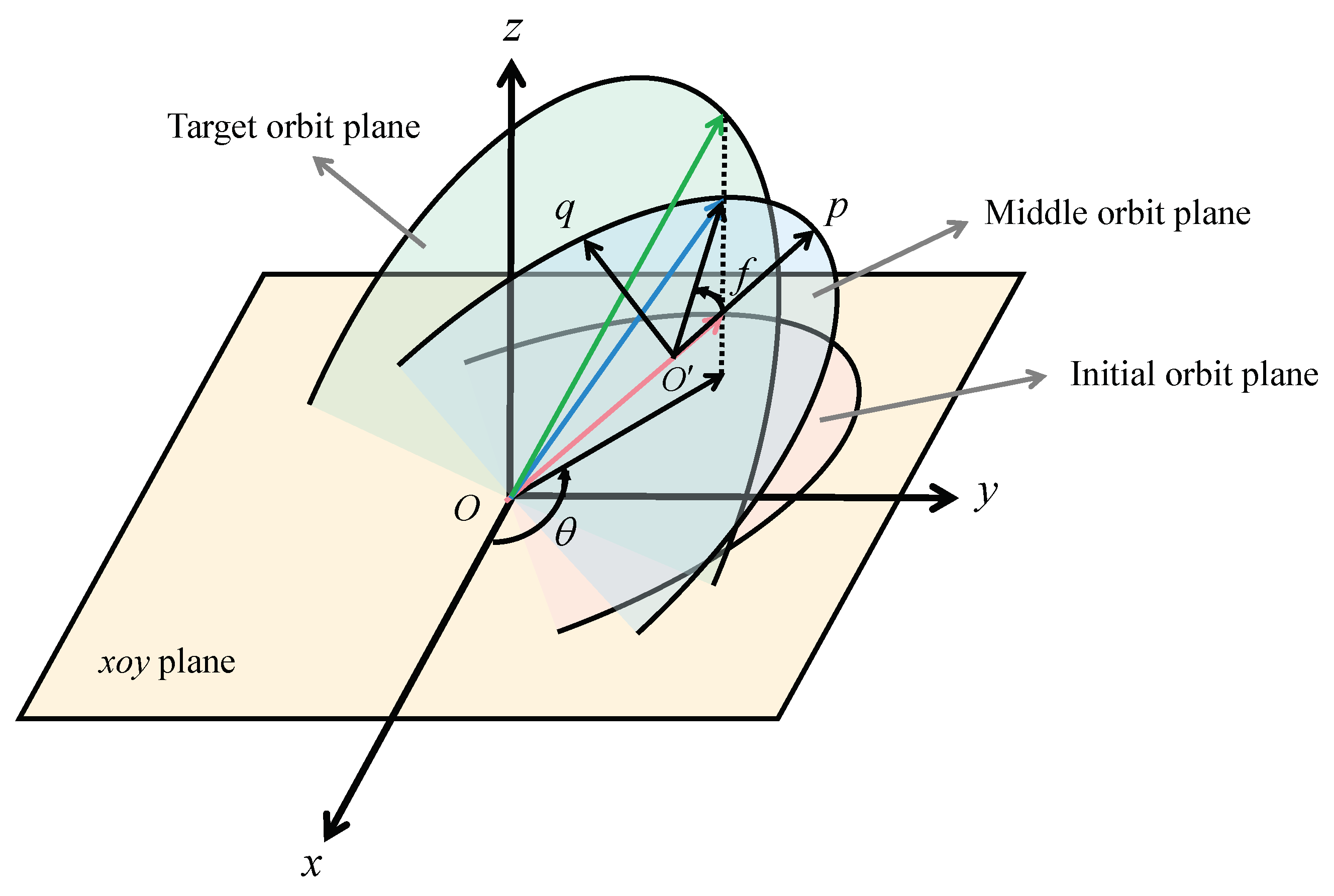
Equation (8) is firstly proposed for the case of a rev2D trajectory, where is the parameter in polar coordinates. For the 3D case with a large elevation angle, the corresponding true anomaly shown in Figure 2 changes sharply with respect to the azimuthal angle around the descending/ascending nodes. In this case, the radius obtained by Equation (8), which is intentionally designed for the 2D case, is unreasonable around these nodes. Thus, the trajectory is preferred to be parametrized in terms of the true anomaly in the transfer orbital plane compared with the azimuthal angle in the plane. However, considering the difficulty in determining the relationship between the true anomaly of the spacecraft and the azimuthal angle, a compromise strategy is proposed here. Instead of the time-varying transfer orbital plane, a fixed middle orbital plane between the initial and target orbits is used as a reference plane, which can ensure that the angle between the reference plane and the plane is within and avoid the change of the curvature direction of the shape as much as possible when the elevation angle is large. The corresponding true anomaly is given by
As shown in Figure 2, the unit vectors and point to the semi-major and semi-minor axes of the middle orbital plane, respectively, which are obtained by
Accordingly, Equation (8) becomes
2.1.3. Shaping the Time
The unit vectors define the radial–orthoradial–out-of-plane coordinate system [15]. We project the dynamic equations to the tangential–normal–out-of-plane reference frame, which is defined by the unit vectors , and then Equation (2) becomes
where and are the velocity and acceleration vectors in the Cartesian coordinates, respectively, and can be written as
where is the coordinate transformation matrix from the spherical coordinates to the Cartesian coordinates, and and denote the velocity and acceleration vectors in spherical coordinates, respectively. The expressions of , and are obtained by the chain rule:
The detailed formulation of this is given in the Appendix.
Continuous tangent thrust has the advantages of reducing energy consumption in orbit transfer and avoiding the need to change the thrust direction in the orbit plane. It is also convenient for time shaping.Therefore, assuming that there is no normal component of , which is equivalent to , from Equation (12), one can obtain
the expression of D is
The sign of D can represent the curvature direction of the trajectory. Equation. (20) requires that D must be positive, which means that the trajectory must bend towards the central celestial body.
Combining Equation (12) and Equation (20), the velocity increment during the orbit transfer can be obtained as
The angular acceleration is contained in , which can be calculated as
where
and are also obtained by the chain rule, the details of which are shown in Appendix A.
2.2. Determination of Shaping Functions
To determine the interpolation function and the seven unknown coefficients for the radius shape, the trajectory boundary constraints and non-intersect constraint are analyzed in this subsection. The boundary constraints on the rendezvous trajectory consist of 11 shape boundary constraints (including the initial states , the final states , and the transfer time ) and the fixed initial and final independent variables . Meanwhile, the unknown coefficients for the radius shape are designed to satisfy the constraints on , whereas the constraints on will be satisfied by the interpolation function in combination with another four free parameters.
2.2.1. Determination of Interpolation Function
The constraints on the elevation angle are satisfied by
The interpolation function takes the value of 1 when and 0 when . Since the initial and final velocities of the spacecraft out of orbital planes are zeros, the derivatives are zeros at and .
Suppose that the initial and target orbits do not intersect for any ; the angle of the transfer orbits is designed between that of the initial and target orbits (viz. trajectory safety in [18]), which can avoid collision and save energy to a certain extent. Therefore, a monotonic decreasing function ( when ) is designed, and its evolution direction is from the initial plane to the target plane.
There are many forms of that can satisfy the above constraints. Considering a reduction of the total velocity increment as much as possible, the transfer orbits have to raise the elevation angle as much as possible at the place with the largest radius and not change the elevation angle as far as possible in the place with a small radius. Therefore, the interpolation functions are given empirically for the cases and , respectively:
If ,
else if ,
where is the normalized parameter, and and are the radial distances of the departure and arrival positions, respectively.
Since the coefficient matrix of and d is linear, they can be obtained analytically by satisfying the boundary conditions:
if
Similarly, if , substituting Equation (25) into Equation (27) gives
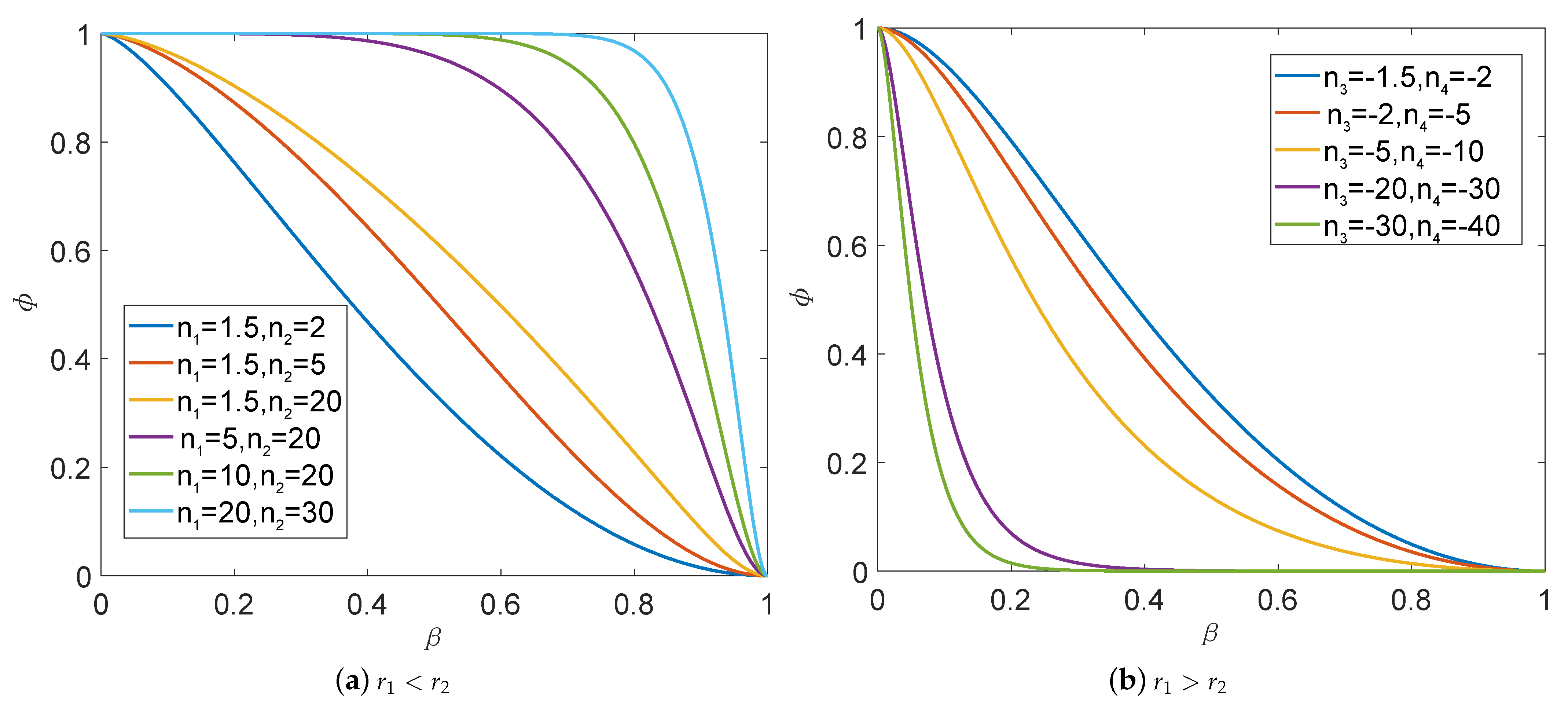
where , , , and are the shaping parameters that shape the trajectory. If the semimajor axes, eccentricities, and inclinations of the initial and final orbits are similar, then the absolute values of , , , and can take small values; for example, from 1 to 10. If the difference is large, then the absolute values of the shaping parameters can take larger values, such as from 10 to 30. Figure 3 shows the evolution of for these different shaping parameters. In practical problems, the shaping parameters are selected by experience, and usually the transfer orbit is designed to raise the elevation angle as much as possible at the place with the largest radius (apogee) in order to reduce fuel consumption. The values of the coefficients selected by experience already have a good effect in the examples, and the results are not sensitive to these coefficients, so there is no further optimization in this paper.
2.2.2. Determination of Coefficients in Radius
It is mentioned in Section 2.1 that the seven coefficients of Equation (11) are used to satisfy seven constraints.
Similarly, at the departure point, it yields
The last constraint is on the time of flight:
All these seven coefficients are required to be solved numerically. The direct estimation of the initial value of the coefficients will lead to a large amount of calculation and difficult convergence. However, if one adjusts the range of the independent variables from to , the analytic solutions of some coefficients can be given according to some boundary conditions. Solving Equations (30) and (31) yields
Then, the number of unknown coefficients will be reduced to 5, which can greatly reduce the computational burden. However, five unknowns and five nonlinear equations correspond to multiple sets of solutions. In this paper, one set of reasonable solutions is sufficient. The fsolve function in Matlab is used to solve , numerically. We set the initial values of all coefficients to 0, then solve the nonlinear equations, and finally obtain a set of reasonable solutions.
3. Application in Indirect Trajectory Optimization
The combination of the indirect method and parameter continuation method [20] can avoid the estimation of the initial value and ensure the convergence of the optimal control problems, but it is necessary to sacrifice the computational efficiency. Directly estimating the initial value of the adjoint variables can improve the computational efficiency, but it is difficult to realize because the indirect method for the trajectory optimization is sensitive to the initial values of the adjoint variables. An adjoint estimation method is proposed in [21] by linearization around a shape-based path. The estimation method improves the convergence rate of the indirect method for coplanar rendezvous trajectory optimization, where the maximum inclination is only . For a general 3D rendezvous with large out-of-plane motion, the estimation performance needs further improvement. In this section, the proposed shape-based method is employed to estimate the initial value of the adjoint variables in combination with the estimation method, of which the convergence rate greatly depends on the shaping approximation. The adjoint normalization is also used to improve the convergence rate. Note that there are two essential evaluation indexes for the shape designed: and . Generally, the smaller the values of and , the closer the trajectory designed by the shape-based method is to that optimized by the indirect method. The low-thrust trajectory optimization model is first introduced, and then the estimation using the proposed shape in the spherical coordinate system is briefly described.
3.1. Optimization Model
The nonlinear optimal control problem with a fixed flight time is given as follows:
Minimize
Subject to
where R is the state vector of the spacecraft, m is the mass of the spacecraft, R and R depend on the coordinate system used, is the engine thrust ratio, is the unit vector of thrust direction, is the standard acceleration of gravity at sea level, and is the thruster-specific impulse. The physical meaning of J in Equation (38) is the total fuel consumption. It is difficult to solve the fuel-optimal problem directly because of the bang-bang structure. The homotopy method provides an idea by adding a homotopic parameter to the index [19,22]. The new performance index is
By reducing from 1 to 0, the energy-optimal problem can be connected with the fuel-optimal problem, which is called the continuation technique for homotopic problems. In the process of reducing , the solution of the previous step is always taken as the initial estimated value of the current step. Only when = 0 will the difficult bang-bang control appear. In other cases, the optimal control law is continuous.
In the homotopic process, when the parameter is close to 0, the right hand sides of the ODEs vary rapidly around the switching points. The numerical integrator should be carefully performed when crossing these points. Here, for simplicity of operation, a fixed step integrator with switching function detection rather than an adaptive step size integrator is used [19].
Obviously, when = 1, Equation (40) becomes the energy-optimal index:
In the next subsection, based on the problem of energy-optimal problem, the combination of the indirect method and shape-based method is discussed.
3.2. Adjoint Estimation Based on Shape-Based Method
This subsection is similar to the problem formulation in [21], which is established accordingly in the cylindrical coordinates [23] and then combined with the indirect method of the optimization problem to obtain the corresponding solution.
The cylindrical coordinates are selected because experience shows that solving the optimization problem in the cylindrical coordinates results in a higher convergence rate than that in the spherical coordinates. Therefore, in practice, it is necessary to convert the shape (nominal trajectory) from the spherical coordinates to the cylindrical coordinates through the coordinate conversion method.
We denote the combination coordinates of position and velocity expressed in the cylindrical coordinates by , and their corresponding adjoint variables by . After linearizing the motion equation near the nominal trajectory which is designed in Section 2 and taking the energy-optimal problem as the one that needs to be solved, the motion equations and Euler–Lagrange equations with as the independent variable are derived:
where
where and represent the state and acceleration of the nominal trajectory, respectively. is the Jacobian matrix of the central gravitational acceleration:
where represents the distance between the central celestial body and the spacecraft.
We denote as
Let . Then, the initial adjoint variables can be expressed as
The nominal trajectory designed in Section 2 has already met the boundary conditions, which means = 0 and = 0, so Equation (48) can be simplified as
The mass adjoint variable is given by integrating the following equation:
3.3. Adjoint Normalization
In practice, it can be found that the method in Section 3.2 cannot significantly improve the convergence rate when the shapes of the initial and target orbits differ greatly. This subsection introduces the normalization method [19] based on Section 3.2 to improve the convergence rate.
Multiplying the index Equation (41) by a positive multiplier does not change the essence of the problem. Consequently, the updated Hamiltonian function is expressed as
where is the group of the last three components of .
Therefore, the normalized adjoint variables and can be expressed as
where the positive multiplier is obtained according to the normalization condition:
In practice, the initial mass adjoint is randomly selected between 0 and the estimated value [21].
4. Numerical Examples
In this section, three orbit rendezvous examples are given to verify the feasibility and advantages of the shape-based method proposed. The Novak method has the limitation of the elevation angle, which means that it fails to obtain a feasible solution when the elevation angle is large. The proposed method is not affected by the inclination of the initial and target orbits and can generate an arbitrary 3D rendezvous trajectory. Compared with the Zeng method, the proposed method can greatly reduce the velocity increment and the , which indicates that the rendezvous trajectory generated by the proposed method is closer to the optimal trajectory. The first two examples illustrate the advantages mentioned above. As for the third example, the trajectory generated by the proposed method is combined with the indirect method and the adjoint normalization to prove that it can broaden the convergence range and improve the convergence efficiency of rendezvous problems. All the examples were performed on a personal desktop with an Intel Core i7-7700 CPU of 3.6 GHz and 8.00 GB of RAM and with MATLAB R2018a.
Nondimensionalization was performed by setting the length unit to the astronomical unit (AU), the time unit, denoted by TU, to of the period of a circular orbit with radius 1 AU, and the mass unit, denoted by MU, to the initial mass of the spacecraft. Furthermore, the new velocity unit is denoted by VU.
4.1. Rendezvous Mission A from Inner Orbit to Outer Orbit
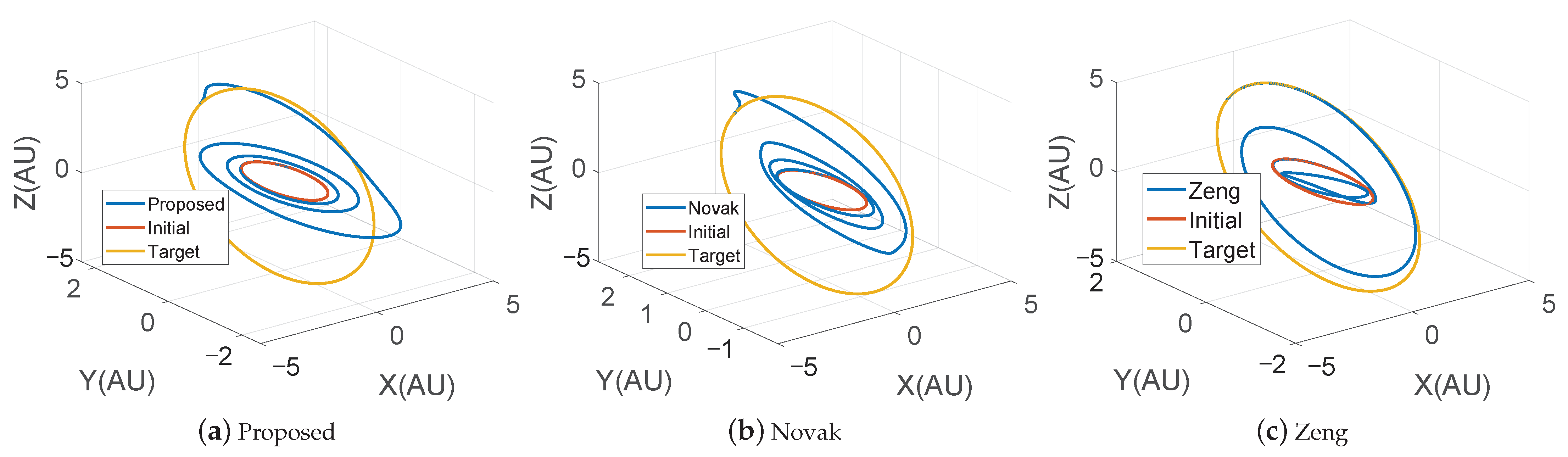
The initial and target orbit elements of mission A are listed in Table 1. The elevation angle is set to to verify the feasibility and efficiency of the proposed shape for the 3D rendezvous. The semi-major axis is set from 1 to 4, and the eccentricity is set from 0 to 0.1, which can be used to prove the ability to perform an elliptic rendezvous. Assume that the revolution number N is 3, the fixed flight time is 9 years (56.5089 TU), and the shaping parameters are 10 and 20 for and , respectively. The shaping parameters are chosen according to experience in order to raise the elevation angle at the place with the largest radius as much as possible.
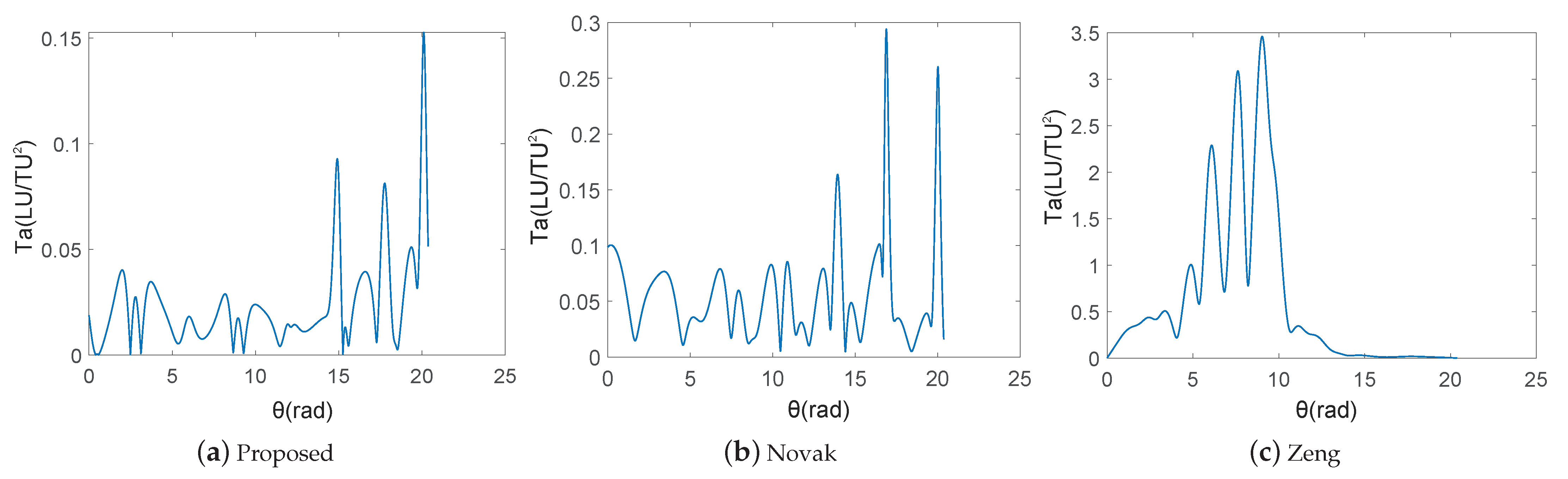
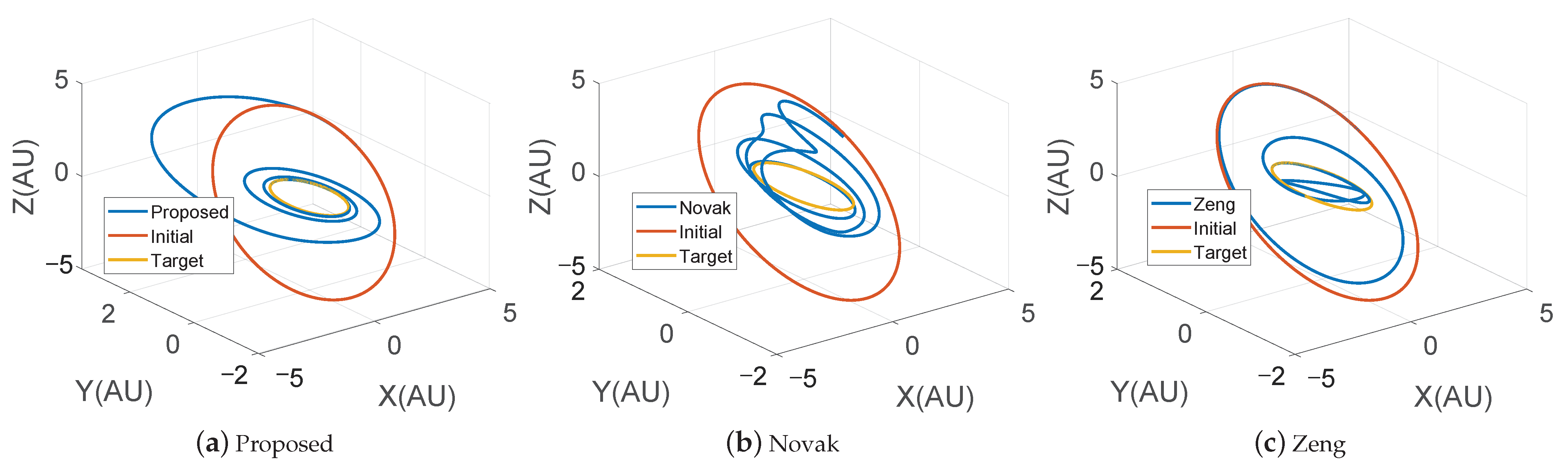
Then, the trajectories obtained by the three methods are shown by Figure 4 and Figure 5. The velocity increment and the maximal thrust acceleration of each method are listed in Table 2. Compared with Novak’s method and Zeng’s method, the proposed method saves by and , respectively, which greatly reduces the fuel consumption in rendezvous problems. The maximal thrust acceleration is also significantly reduced from Zeng’s method, at 3.458, and Novak’s method, at 0.2943, to the proposed method’s result of 0.1527.
The longer the rendezvous time, the easier it is to solve the rendezvous trajectory, which can test the flexibility of the rendezvous shape. By adjusting the rendezvous time and keeping other parameters unchanged, we obtain the results listed in Table 3, where N/A means no solution. This shows that whether the rendezvous time is long or short, the proposed method always has the minimum and the minimum . Zeng’s method has no solution when the rendezvous time is short. This is because Zeng’s method does not consider the monotonicity of and but uses safety as a reference quantity to test the quality of the trajectories. Thus, there may be no solution when the rendezvous time is too short. Moreover, the safety of trajectories is considered by the proposed method in the design of the elevation angle, but it is not considered in the design of the radius. Hence, the trajectories may intersect with each other when the rendezvous time is shortened.
Let the rendezvous time be 9 years (56.5089 TU), N = 3, and the orbit elements except the orbital inclination are the same as the above example. Table 4 lists the results. This shows that the proposed method is superior to the existing two methods when the elevation angle is large. In addition, Novak’s method often fails when both the initial and target orbital inclination, and , are larger than . Moreover, when , the rendezvous trajectories designed by Novak’s method are not in the same plane because the projection problem of the true anomaly and azimuthal angle is not considered. Although Zeng’s method is feasible at all elevation-angles, and cannot be reduced.
4.2. Rendezvous Mission B from Outer Orbit to Inner Orbit
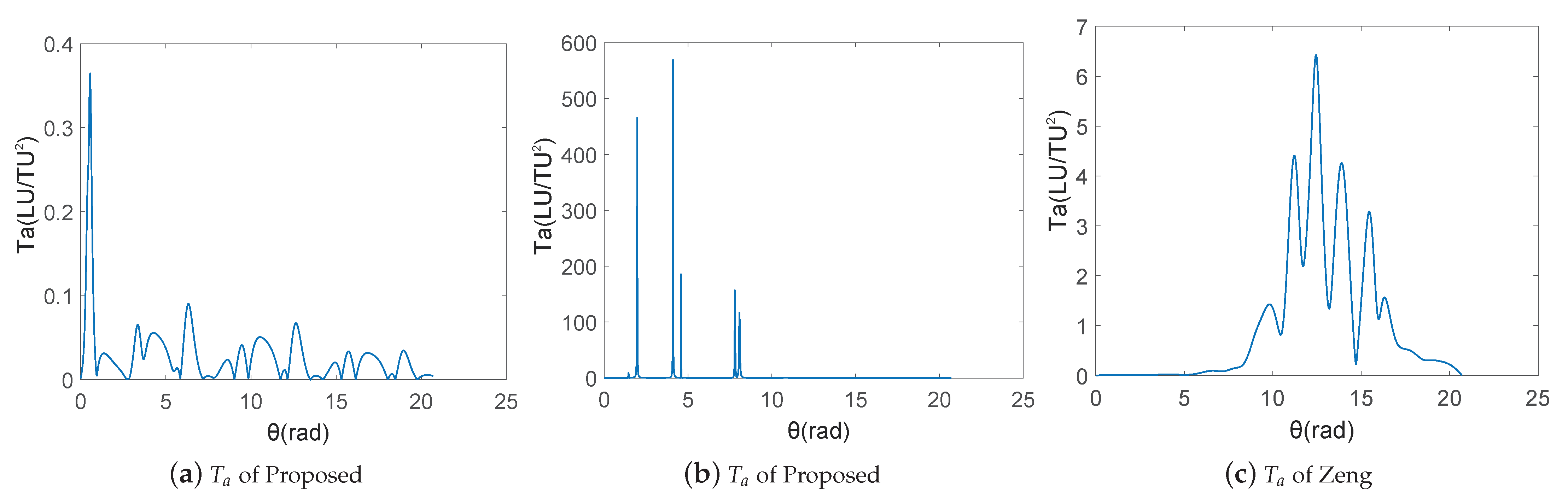
For mission B, the semi-major axes, eccentricities, and orbital inclinations of the initial and target orbit elements are set to be the same as those for mission A, respectively, which are also listed in Table 1. Let N = 3, = 9 years (56.5089 TU), = −20 and = −30. The trajectories are shown in Figure 6, and the results are listed in Table 5. Obviously, in this rendezvous problem, Novak’s method has no solution. The trajectory designed by Zeng’s method intersects itself, and both the velocity increment and maximal thrust acceleration are large. The proposed method is to transform the elevation angle as far as possible at the place with the largest radius, so it can be seen from Figure 7 that there will be a relatively large thrust acceleration level in the initial stage of rendezvous, but compared with Zeng’s method, its and are small.
4.3. Adjoint Estimation with Shape-Based Method
The velocity increment and maximal thrust acceleration of the rendezvous trajectories designed by Zeng’s method are large and intersect themselves in many cases, so they are not suitable to be used as the nominal trajectories. The following only compares the performance of the nominal trajectories designed by the proposed method with Novak’s method. Both MaxFunEvals and MaxIter options of the fsolve function in Matlab R2018a are set to 2000.
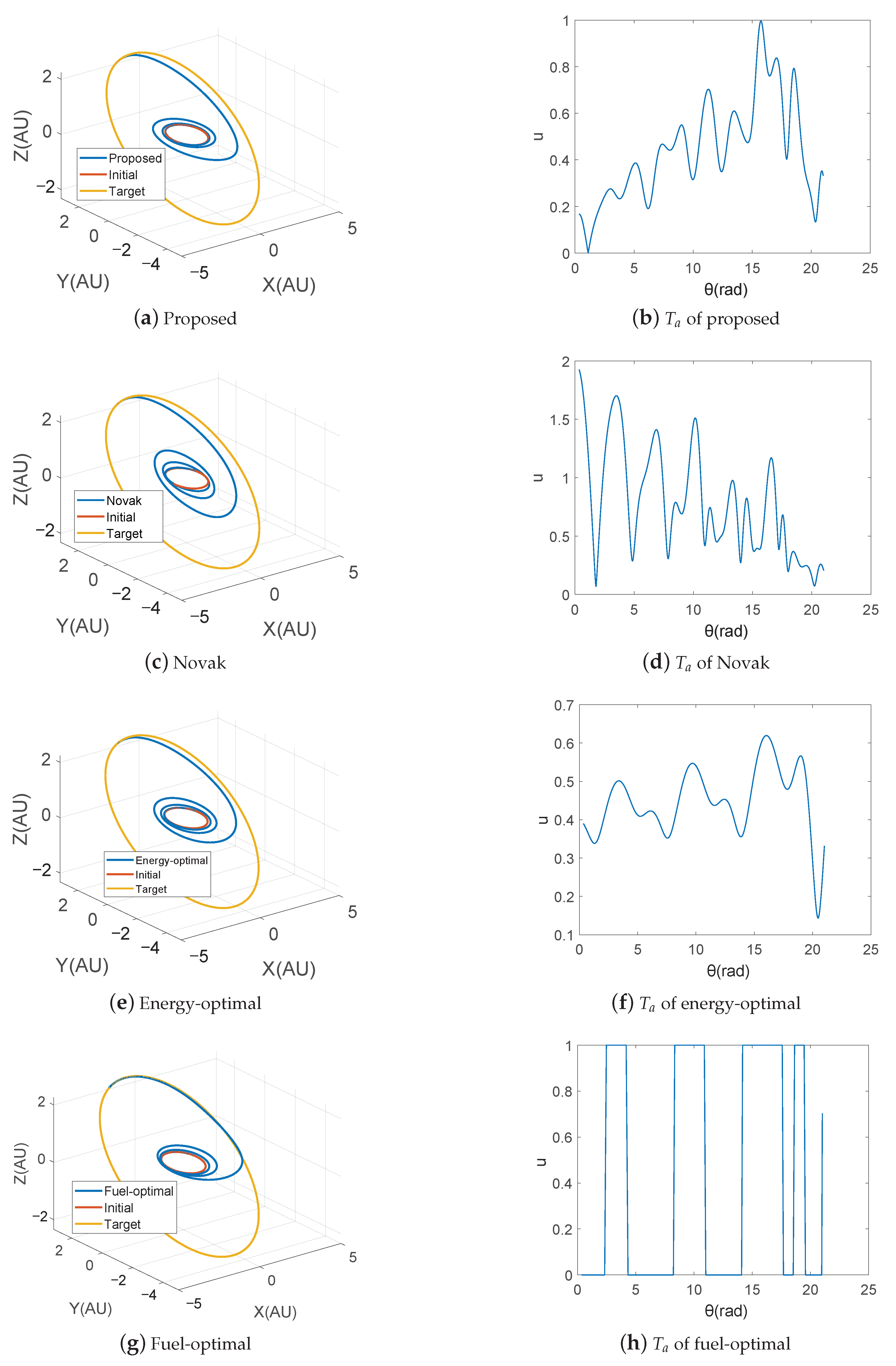
We consider mission A and make the orbit elements the same as those of mission A in Table 1 except . Let be , N be 3 and be 7 years (43.9514TU). The spacecraft performance parameters are listed in Table 6. Here, we use the percentage of converged (POC) cases out of 100 samples to evaluate the nominal trajectories. The only difference between these 100 examples is that the initial adjoint of mass is randomly selected between 0 and the estimated value [21]. Table 7 reports the POC and the initial values of the adjoint variables and estimated by each method with different nominal trajectories. It also shows the actual initial adjoint variables of the energy-optimal problem. The initial adjoint variables of the fuel-optimal problem are obtained by the homotopic approach based on the energy-optimal problem. Figure 8 shows the shape and normalized thrust generated by each method.
Table 7 shows that the POC of the proposed method is higher than Novak’s method, because the trajectory designed by the proposed method is closer to the energy-optimal trajectory in shape than that designed by Novak’s method; it also consumes less and has smaller . At the same time, compared with the non-normalized adjoint variables, the POC of the normalized adjoint variables has been significantly improved.
Table 8 presents the simulation results for cases where only the of the target orbit is changed, while other parameters are kept unchanged. It can be seen that when the adjoint variables are not normalized, the POC of Novak’s method is higher than that of the proposed method in the case of a small elevation angle, but Novak’s method is not applicable in the case of a large elevation angle. When the adjoint variables are normalized, the POC of the two methods is significantly improved, and the POC of the proposed method is significantly higher than that of Novak’s method.
5. Conclusions
This paper proposed a new shape-based method to solve 3D rendezvous problems, keeping the advantages of Novak’s method and Zeng’s method. It also improves the out-of-plane shaping functions, which makes the proposed rendezvous trajectories more flexible and more applicable. The proposed method can generate an arbitrary 3D rendezvous trajectory and can significantly reduce the velocity increment and maximal thrust acceleration for most test cases. Compared with other shape-based methods, the proposed method does not need to optimize free parameters. At the same time, this paper adds the adjoint normalization into the process of combining the shape-based method with the optimization problem and takes the proposed trajectories as the nominal orbits to provide the initial estimates of the adjoint variables for the indirect method. It is proved that the shape-based method proposed in this paper can be effectively applied to the optimization problems of orbital rendezvous problems when the inclinations of the initial and target orbits differ greatly.
Author Contributions
T.Z. and D.W. completed preliminary research and provided the numerical part; T.Z. and F.J. conceived and wrote the paper; F.J. and H.Z. supervised the overall work and reviewed the paper. All authors have read and agreed to the published version of the manuscript.
Funding
This work was supported by the National Natural Science Foundation of China (No. 12022214).
Institutional Review Board Statement
Not applicable.
Informed Consent Statement
Not applicable.
Data Availability Statement
The data presented in this study are available on request from the corresponding author.
Conflicts of Interest
The authors declare no conflict of interest.
Appendix A
This Appendix shows the expressions of , , , , , and .
The derivative and double derivative of with respect to can be expressed as
, , , j=1,2 are defined as
The derivative and double derivative of the interpolation function are
if
if
Let denote the denominator of r, and , , and denote the derivative, double derivative, and triple derivative of the denominator of r with respect to f, respectively:
Then, , , and are
where
, , and are denoted as
References
- Betts, J. Survey of Numerical Methods for Trajectory Optimization. J. Guid. Control. Dyn. 1998, 21, 193–207. [Google Scholar] [CrossRef]
- David, G.H. Conversion of Optimal Control Problems into Parameter Optimization Problems. J. Guid. Control. Dyn. 1997, 20, 57–60. [Google Scholar]
- Caruso, A.; Quarta, A.A.; Mengali, G. Comparison between Direct and Indirect Approach to Solar Sail Circle-to-circle Orbit Raising Optimization. Astrodynamics 2019, 3, 273–284. [Google Scholar] [CrossRef]
- Yan, H.; Wu, H. Initial Adjoint-Variable Guess Technique and Its Application in Optimal Orbital Transfer. J. Guid. Control. Dyn. 1999, 22, 490–492. [Google Scholar] [CrossRef]
- Mantia, M.; Casalino, L. Indirect Optimization of Low-Thrust Capture Trajectories. J. Guid. Control. Dyn. 2006, 29, 1011–1014. [Google Scholar] [CrossRef]
- Martell, C.A.; Lawton, J.A. Adjoint Variable Solutions via an Auxiliary Optimization Problem. J. Guid. Control. Dyn. 2015, 18, 1267–1272. [Google Scholar] [CrossRef]
- Kluever, C.A.; Pierson, B.L. Optimal Low-Thrust Earth-Moon Transfers with a Switching Function Structure. J. Astronaut. Sci. 1994, 42, 269–283. [Google Scholar]
- Kluever, C.A.; Pierson, B.L. Optimal Low-thrust Three-Dimensional Earth-Moon Trajectories. J. Guid. Control Dyn. 1995, 18, 830–837. [Google Scholar] [CrossRef]
- Gao, Y.; Kluever, C. Low-Thrust Interplanetary Orbit Transfers Using Hybrid Trajectory Optimization Method with Multiple Shooting. In Proceedings of the AIAA/AAS Astrodynamics Specialist Conference and Exhibit, Providence, RI, USA, 16–19 August 2004. [Google Scholar]
- Yang, H.; Tang, G.; Jiang, F. Optimization of Observing Sequence Based on Nominal Trajectories of Symmetric Observing Configuration. Astrodynamics 2018, 107, 25–37. [Google Scholar] [CrossRef]
- Petropoulos, A.E.; Longuski, J.M. Shape-Based Algorithm for the Automated Design of Low-Thrust, Gravity Assist Trajectories. J. Spacecr. Rocket. 2004, 41, 787–796. [Google Scholar] [CrossRef] [Green Version]
- Wall, B.J.; Conway, B.A. Shape-Based Approach to Low-Thrust Rendezvous Trajectory Design. J. Guid. Control. Dyn. 2009, 32, 95–101. [Google Scholar] [CrossRef]
- Wall, B.J.; Pols, B.; Lanktree, B. Shape-based Approximation Method for Low-thrust Interception and Rendezvous Trajectory Design. Adv. Astronaut. Sci. 2010, 136, 1447–1458. [Google Scholar]
- Wall, B.J. Shape-Based Approximation Method for Low-Thrust Trajectory Optimization. In Proceedings of the AIAA/AAS Astrodynamics Specialist Conference and Exhibit, Honolulu, HI, USA, 18–21 August 2008. [Google Scholar]
- Novak, D.M.; Vasile, M. Improved Shaping Approach to the Preliminary Design of Low-Thrust Trajectories. J. Guid. Control. Dyn. 2011, 34, 128–147. [Google Scholar] [CrossRef] [Green Version]
- Xie, C.; Zhang, G.; Zhang, Y. Simple Shaping Approximation for Low-Thrust Trajectories Between Coplanar Elliptical Orbits. J. Guid. Control. Dyn. 2015, 38, 2448–2455. [Google Scholar] [CrossRef]
- Xie, C.; Zhang, G.; Zhang, Y. Shaping Approximation for Low-Thrust Trajectories with Large Out-of-Plane Motion. J. Guid. Control Dyn. 2016, 39, 2776–2786. [Google Scholar] [CrossRef]
- Zeng, K.; Geng, Y.; Wu, B. Shape-Based Analytic Safe Trajectory Design for Spacecraft Equipped with Low-Thrust Engines. Aerosp. Sci. Technol. 2017, 62, 87–97. [Google Scholar] [CrossRef]
- Jiang, F.; Baoyin, H.; Li, J. Practical Techniques for Low-Thrust Trajectory Optimization with Homotopic Approach. J. Guid. Control. Dyn. 2012, 35, 245–258. [Google Scholar] [CrossRef]
- Petukhov, V.G. Optimization of Interplanetary Trajectories for Spacecraft with Ideally Regulated Engines Using the Continuation Method. Cosm. Res. 2008, 46, 219–232. [Google Scholar] [CrossRef]
- Jiang, F.; Tang, G.; Li, J. Improving Low-Thrust Trajectory Optimization by Adjoint Estimation with Shape-Based Path. J. Guid. Control. Dyn. 2017, 40, 1–8. [Google Scholar] [CrossRef]
- Taheri, E.; Kolmanovsky, I.; Atkins, E. Enhanced Smoothing Technique for Indirect Optimization of Minimum-Fuel Low-Thrust Trajectories. J. Guid. Control. Dyn. 2016, 39, 2500–2511. [Google Scholar] [CrossRef] [Green Version]
- Lewallen, J.M.; Schwausch, O.A.; Tapley, B.D. Coordinate System Influence on the Regularized Trajectory Optimization Problem. J. Spacecr. Rocket. 1971, 8, 15–20. [Google Scholar] [CrossRef] [Green Version]
Figure 1.
Illustration of the spherical coordinates.

Figure 2.
Diagram of the relationship between f and .

Figure 3.
Effect of the shaping parameters on .

Figure 4.
Rendezvous results of three methods when .

Figure 5.
Thrust acceleration of three methods when .

Figure 6.
Rendezvous result of three methods when .

Figure 7.
Thrust acceleration of each method when .

Figure 8.
Rendezvous result of three methods.


Table 1.
Orbit elements of two missions.
| Mission A () | Mission B () | |||
|---|---|---|---|---|
| Orbit Elements | Initial Orbit | Target Orbit | Initial Orbit | Target Orbit |
| Semi-major axis | 1 | 4 | 4 | 1 |
| Eccentricity | 0.01 | 0.1 | 0.1 | 0.01 |
| Inclination | ||||
| Right ascension | ||||
| Argument of periapsis | ||||
| True anomaly |
Table 2.
Orbit rendezvous results when .
| Method | (VU) | () |
|---|---|---|
| Proposed | 1.5938 | 0.1527 |
| Novak | 2.8070 | 0.2943 |
| Zeng | 10.2439 | 3.4581 |
Table 3.
Orbit rendezvous results with different when .
| Proposed | Novak | Zeng | ||||
|---|---|---|---|---|---|---|
| (VU) | () | (VU) | () | (VU) | () | |
| 90 | 1.7764 | 0.2229 | N/A | N/A | 2.4425 | 0.2997 |
| 80 | 1.7060 | 0.2040 | N/A | N/A | 2.3723 | 0.2442 |
| 70 | 1.6474 | 0.1831 | N/A | N/A | 2.7264 | 0.3755 |
| 60 | 1.6048 | 0.1607 | 2.7395 | 0.2797 | 6.4289 | 1.2344 |
| 50 | 1.5838 | 0.1378 | 3.0000 | 0.5310 | N/A | N/A |
| 40 | 1.7249 | 0.2099 | N/A | N/A | N/A | N/A |
| 30 | 2.3449 | 0.4569 | N/A | N/A | N/A | N/A |
Table 4.
Orbit rendezvous results with different when .
| Proposed | Novak | Zeng | ||||
|---|---|---|---|---|---|---|
| (VU) | () | (VU) | () | (VU) | () | |
| 2.6785 | 0.7977 | N/A | N/A | 9.4952 | 2.4343 | |
| 1.5938 | 0.1527 | 2.8070 | 0.2943 | 10.2439 | 3.4581 | |
| 1.1906 | 0.0651 | 1.8830 | 0.1006 | 10.2524 | 4.1412 | |
| 0.9553 | 0.0381 | 1.2862 | 0.0706 | 9.8555 | 4.6166 | |
| 0.7887 | 0.0257 | 0.8931 | 0.0548 | 9.2535 | 5.0227 | |
| 0.6539 | 0.0228 | 0.6582 | 0.0393 | 8.6234 | 5.7724 | |
| 0.5465 | 0.0212 | 0.5384 | 0.0256 | 8.1394 | 7.2918 |
Table 5.
Orbit rendezvous results when .
| Method | (VU) | () |
|---|---|---|
| Proposed | 1.8345 | 0.3646 |
| Novak | N/A | N/A |
| Zeng | 14.2508 | 6.4255 |
Table 6.
Spacecraft performance parameters.
| 3000 | 0.8 | 5000 |
Table 7.
Initial costates and POC of different methods.
| Method | POC | ||
|---|---|---|---|
| Proposed | |||
| Proposed (normalization) | |||
| Novak | |||
| Novak (normalization) | |||
| Energy-optimal | N/A | ||
| Fuel-optimal | N/A |
Table 8.
POC of different methods with different .
| Proposed | Proposed (Normalization) | Novak | Novak (Normalization) | |
|---|---|---|---|---|
| N/A | N/A | |||
| N/A | N/A | |||
Publisher’s Note: MDPI stays neutral with regard to jurisdictional claims in published maps and institutional affiliations. |
© 2021 by the authors. Licensee MDPI, Basel, Switzerland. This article is an open access article distributed under the terms and conditions of the Creative Commons Attribution (CC BY) license (https://creativecommons.org/licenses/by/4.0/).
Share and Cite
MDPI and ACS Style
Zhang, T.; Wu, D.; Jiang, F.; Zhou, H. A New 3D Shaping Method for Low-Thrust Trajectories between Non-Intersect Orbits. Aerospace 2021, 8, 315. https://0-doi-org.brum.beds.ac.uk/10.3390/aerospace8110315
AMA Style
Zhang T, Wu D, Jiang F, Zhou H. A New 3D Shaping Method for Low-Thrust Trajectories between Non-Intersect Orbits. Aerospace. 2021; 8(11):315. https://0-doi-org.brum.beds.ac.uk/10.3390/aerospace8110315
Chicago/Turabian StyleZhang, Tongxin, Di Wu, Fanghua Jiang, and Hong Zhou. 2021. "A New 3D Shaping Method for Low-Thrust Trajectories between Non-Intersect Orbits" Aerospace 8, no. 11: 315. https://0-doi-org.brum.beds.ac.uk/10.3390/aerospace8110315
Note that from the first issue of 2016, this journal uses article numbers instead of page numbers. See further details here.