A Novel Performance Adaptation and Diagnostic Method for Aero-Engines Based on the Aerothermodynamic Inverse Model

Abstract

Aero-engines are faced with severe challenges of availability and reliability in the increasing operation, and traditional gas path filtering diagnostic methods have limitations restricted by various factors such as strong nonlinearity of the system and lack of critical sensor information. A method based on the aerothermodynamic inverse model (AIM) is proposed to improve the adaptation accuracy and fault diagnostic dynamic estimation response speed in this paper. Thermodynamic mechanisms are utilized to develop AIM, and scaling factors are designed to be calculated iteratively in the presence of measurement correction. In addition, the proposed method is implemented in combination with compensation of the nonlinear filter for real-time estimation of health parameters under the hypothesis of estimated dimensionality reduction. Simulations involved experimental datasets revealed that the maximum average simulated error decreased from 13.73% to 0.46% through adaptation. It was also shown that the dynamic estimated convergence time of the improved diagnostic method reached 2.183 s decrease averagely without divergence compared to the traditional diagnostic method. This paper demonstrates the proposed method has the capacity to generalize aero-engine adaptation approaches and to achieve unbiased estimation with fast convergence in performance diagnostic techniques.

1. Introduction

Aero-engine is an aerothermodynamic system with a complicated structure and strong nonlinearity. It works in harsh environments with high temperatures, high pressures and high rotating speeds for extended periods of time, which results into the inevitable degradation of components. Once the performance failure and abrupt malfunction occur in the power plant of the flight vehicle, it causes substantial economic losses and has a high probability of initiating catastrophic accidents [1]. Therefore, an effective maintenance is essential to maintain a high level of availability and reliability of aero-engines. With the development of engine health monitoring technologies, gas path fault diagnosis of a component or a system has become an aera of interest in the field of flight propulsion researches [2].

Aero-engine gas path fault diagnosis can be divided into three categories: model-based approach, data-driven approach, and information fusion approach [3], wherein model-based diagnostic method is a practical tool with respect to on-board implementation considerations and low model complexity. The method depends on the thermodynamic model of the aero-engine, and the modeling accuracy directly determines the diagnostic effectiveness. Consequently, an accurate mathematical model plays a vital role in the successful gas path diagnosis.

Various adaptation techniques have been employed for the goal mentioned above. Data-based adaptation methods such as neural networks [4,5] or function fitting [6,7] are frequently applied to the generation of the engine component performance maps. However, these methods require large amounts of experimental data that have limited availability due to proprietary issues and liability. Another more commonly used method involves scaling and shifting the shape of reference component maps to best match the engine model and target measurement. Stamatis et al. defined a set of scaling factors to modify the component maps iteratively to increase the performance model accuracy [8]. From this foundation, Kong et al. distinguished operating conditions between the design point (DP) and off-design (OD) points for independent modification based on system identification [9]. To avoid blindness in the adaptation process, optimization algorithms have been implemented extensively for the fittest solution among all potential solutions. Kong et al. used a genetic algorithm (GA) to obtain more accurate component maps from experimental data [10]. Li et al. introduced quadratic function representing nonlinear scaling factors to produce modifications for different speed lines using GA [11]. Tsoutsanis et al. considered rotation of the ellipses and transformation of its coordinates, where the shape of a compressor map was expressed by the mathematical equations of an ellipse with a fixed center and no rotation [12]. The Nelder–Mead algorithm was implemented to ensure the minimum of the objective function [13]. Nevertheless, the advantages and benefits of the above approaches for performance adaptation are extensive. It is hard to trade off key parameters such as accuracy, local optimum, and computational time.

The performance diagnosis of the aero-engine is a more challenging task with deep-rooted and underlying problems, and it provides crucial support for the engine security, reliability and economy. With the help of an accurate engine model, abundant technologies relevant to model-based diagnosis are studied. Urban first introduced a gas path analysis (GPA) method for a linear approximation at a certain operating point, and it can detect different fault modes with a small quantity of fault coefficients [14]. Multiple diagnostic systems based on GPA have been developed so far, such as TEMPER [15] and MAPNET [16]. In addition, Bai introduced a robust state estimation method with the internal searching optimized by GA [17]. Brotherton et al. introduced a diagnostic method for the subset of the health parameters against multicollinearity [18].

In recent decades, the Kalman filter (KF) has attracted much attention due to its easy implementation and optimal estimation performance under a Gaussian white noise environment. Linear KF (LKF) was used by Simon for gas path fault estimation with constraints such as linear inequalities [19] and density functions [20] to improve accuracy and stability. Nonlinear KFs, an extension of KF, developed rapidly in the application of the nonlinear system. Several forms such as Extended KF (EKF) [21], Unscented KF (UKF) [22] and Cubature KF (CKF) [23], had better state estimation accuracy for gas turbine engines when compared to LKF [24,25,26,27]. Kobayashi used EKF for the performance parameter estimation on a turbofan engine [28]. Dewallef studied online performance monitoring and diagnostic technologies based on UKF [29]. Yang et al. proposed a hybrid KF to improve the fault detection and isolation rates [30]. These previous works mainly focus on detecting gas path fault depending on the statistical properties of parameter variations. In practical engineering, the linearization of a strong nonlinear system cannot always approximate the nonlinearity characteristic of the state equation, leading to the accumulation of estimated errors even divergence with the flight cycles. The lack of critical sensor information generates the diagnostic unreliability. Meanwhile, the nature and quantity of the health parameters calculated at different sampling points may also change due to the change of engine nonlinear features in the transient operating process. These primary problems are the core elements generating high misdiagnosis incidences.

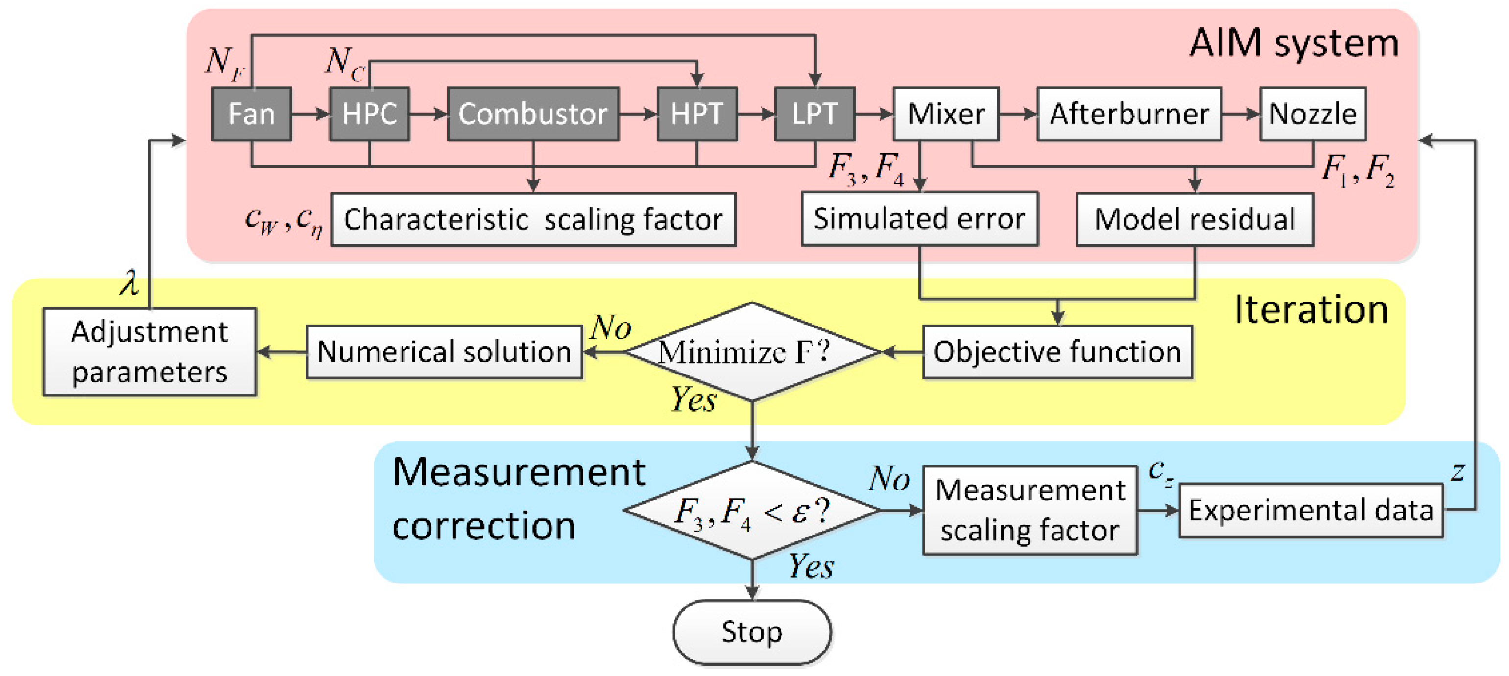
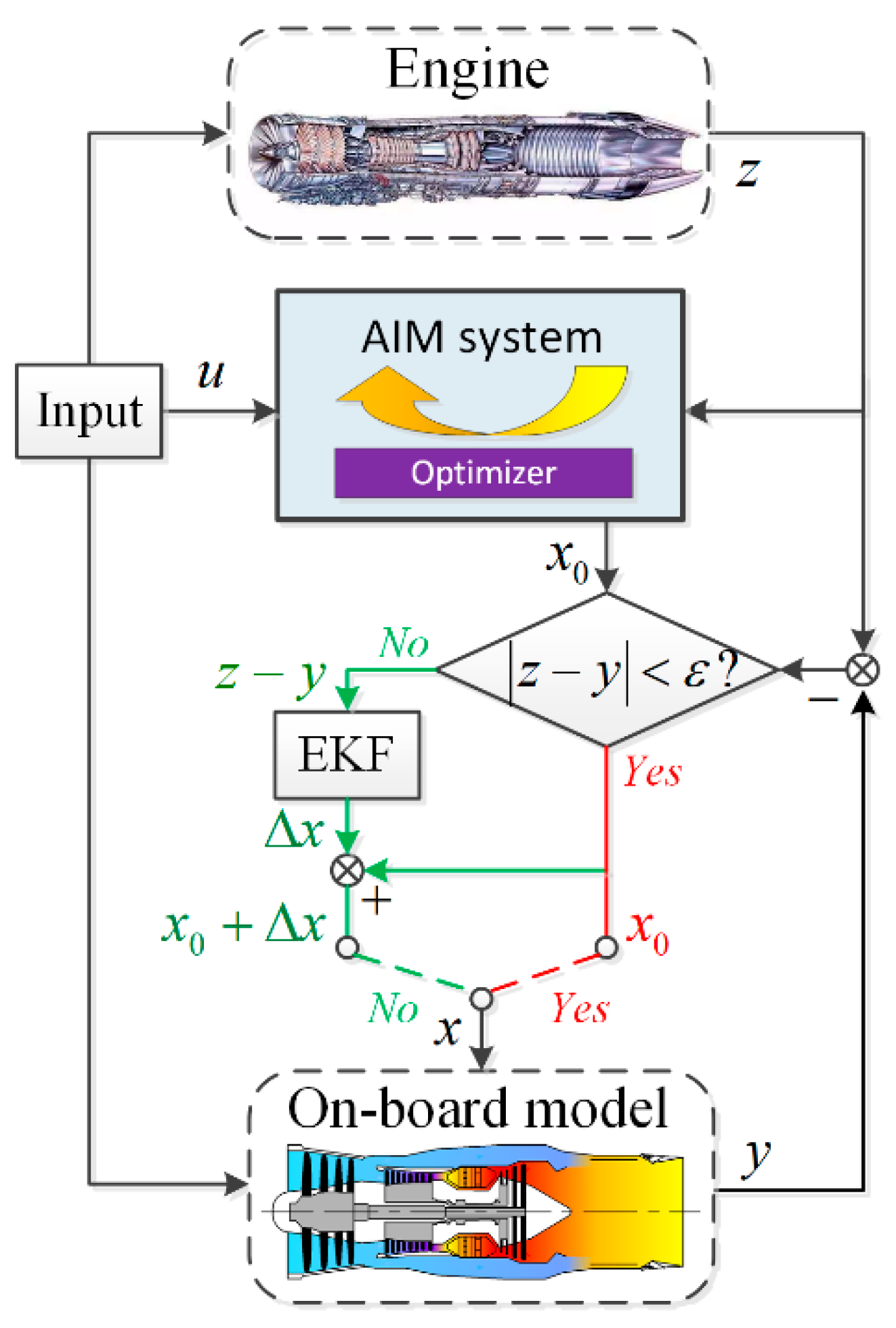
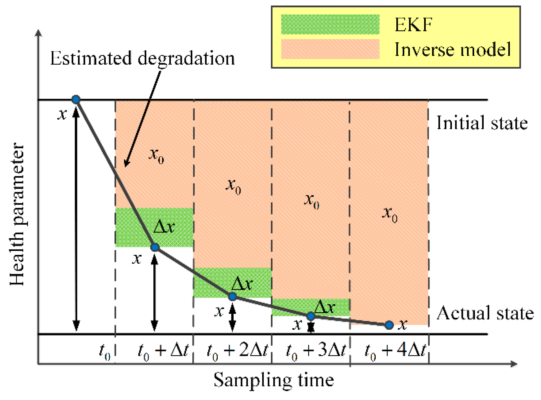
To address this dilemma, the main contribution of this paper proposes a novel method with the capacity to refine model adaptation and performance diagnosis, and it is then integrated into a thermodynamic model of turbofan engine in the development stage. The component aerothermodynamic inverse model (AIM) is established to iteratively calculate measurement and characteristic scaling factors based on multiple experimental data to improve performance prediction accuracy. Besides, due to measurement restrictions, AIM can also be applied to gas path fault diagnostic with the assumption of estimated dimensionality reduction for unbiased estimation. Seven health parameters can be obtained, and compensation is provided using EKF according to the measurement residuals to achieve the real-time diagnosis under transient conditions. The advantages of the proposed method are that the modification achieves high-performance accuracy and low computational cost, which can avoid trapping into local optimum like conventional optimization algorithms. The sensor information also can be utilized adequately for unbiased estimation with fast convergence in fault diagnosis in this method.

This paper is organized as follows: Section 2 introduces the establishment of component AIMs to calculate scaling factors considering measurement correction for model adaptation; Section 3 gives an introduction of computation of health parameters with the compensation of EKF; a set of simulation cases are conducted in Section 4 to test the quality of the proposed performance adaptation and diagnostic method, and Section 5 presents a summary of the research.

2. Model Adaptation

2.1. Measurement Correction

A reliable engine model is the basis of a model-based diagnostic system. The model accuracy is determined by the quality of the measurement. Unfortunately, measured data are usually contaminated by sensor noise, disturbances, instrument degradation and human errors [31]. Hence, measurement correction receives the highest priority during the model adaptation.

The research of this paper focuses on a twin-spool turbofan engine, a reaction engine utilizing high-speed gas flow to generate thrust according to Newton’s laws of motion. The typical components of the engine contain an inlet, a fan, a high-pressure compressor (HPC), a combustor, a high-pressure turbine (HPT), a low-pressure turbine (LPT), a mixing chamber, a bypass, an afterburner, and a nozzle. The configuration of the engine is shown in Figure 1, and the definition of each engine section numbers is listed in

Table 1. Definition of engine section numbers.

Section Number	Definition	Section Number	Definition
2	Fan inlet	6	Core outlet
25	HPC inlet	13	Bypass inlet
3	HPC outlet	16	Bypass outlet
4	Combustor outlet	65	Mixer outlet
45	HPT outlet	7	Nozzle inlet
5	LPT outlet	9	Nozzle outlet

. The turbofan engine has the prominent ability of the complicated structure and numerous condition parameters. Due to the engine geometry construction restriction and hostile operating environments, the parameters about combustor outlet section and HPT outlet section cannot be measured directly. The measurable parameters in the test bench of engine are $n_L$, $n_H$, $P_2$, $T_2$, $P_{25}$, $T_{25}$, $P_3$, $T_3$, $P_6$, $T_6$, $P_{16}$ and $T_{16}$. In addition, the engine control parameters such as fuel flow rate ($W_f$), throat area ($A_8$) and outlet area ($A_9$) of the nozzle can be obtained in the experiment.

Unlike engine component faults, which generally affect changes in a plurality of measurements, the measurement error only results in a single sensor deviation [32]. The case where multiple sensors simultaneously fail rarely occurs. One significant measurement error is considered in this research for greater detection visibility and correction by the appropriate measurement scaling factor $c_z$ defined in Equation (1).

$$c_z=z/z^{\prime },$$

(1)

where $z$ is corrected measurement, and $z^{\prime }$ is uncorrected measurement.

Measurement correction characterizes a sensor error compensation, assisting AIM to achieve optimal and appropriate scaling factors to minimize the measurement errors.

2.2. AIM Establishment

The primary mission of AIM is to generate component characteristic parameters according to the available measured parameters instead of the forward calculation method of the conventional model. To simplify the engine modeling, the influence of combustion delay and energy accumulation is ignored, and gas is assumed as a quasi-one-dimensional flow. AIM is developed by using aerothermodynamic mechanisms for guaranteeing the engine component matching condition. Its objective mainly contains compressor components, a combustor and turbine components. Furthermore, the scaling factors are introduced in a way to implement the model adaptation for quantitatively presentation the degree of component performance deviation.

The following formula derivation takes no account of the engine bleed air system for the sake of convenience. However, the establishment of AIM is an indispensable ingredient to improve calculation accuracy in the practical application. It is worth mentioning that there is no modification for proportion and structure of the air system in order to maintain the original design in this research.

2.2.1. Compressor Component AIM

The compressor components contain the Fan and the HPC. Their operating principle and modeling procedure are similar. The calculation process of the compressor component AIM is shown in Figure 2. Based on the known pressure and temperature in the component inlet and outlet section, the characteristic parameters are calculated as follows:

$$\{\begin{array}{l}\pi =P_{out}/P_{in}\\ h_{in}=f_{T2H}({\gamma }_{in},T_{in})\\ h_{out}=f_{T2H}({\gamma }_{out},T_{out})\\ S_{out}=f_{T2S}({\gamma }_{in},T_{in})+\lg \pi \\ \eta =\left[f_{S2H}({\gamma }_{out},S_{out})-h_{in}\right]/\left(h_{out}-h_{in}\right)\end{array},$$

(2)

where $f_{T2H}$ denotes the function calculating the gas specific enthalpy from its temperature, $f_{T2S}$ denotes the function calculating the gas specific entropy from its temperature, and $f_{H2S}$ denotes the function calculating the gas specific entropy from its specific enthalpy.

Assuming that the air mass flow of the compressor component has been determined as an adjustment parameter, the consumption power can be calculated from Equation (3).

$$N=W_{in}(h_{out}-h_{in})$$

(3)

The scaling factors are calculated to modify the compressor component characteristics:

$$\{\begin{array}{l}{n}_{cor}=\left(n/\sqrt{T_{in}}\right)/\left(n_d/\sqrt{T_{in,d}}\right)\\ c_W=\frac{W_{in}{P}_{in,d}}{f_{map,W}(n_{cor},\pi )P_{in}}\sqrt{\frac{T_{in}}{T_{in,d}}}\\ c_{\eta }=\eta /f_{map,\eta }(n_{cor},\pi )\end{array},$$

(4)

where $f_{map,W}$ and $f_{map,\eta }$ denote the interpolation function of the performance map of mass flow capacity and efficiency, respectively.

2.2.2. Combustor AIM

The combustor computes the stagnation temperature rise from a specified input fuel flow. The combustor’s high temperature leads to outlet measurement difficulties. To estimate characteristic parameters such as combustion efficiency, the components between the inlet and mixing chamber can be viewed as a whole. The calculation principle is shown in Figure 3, where adjustment parameters are indicated by dotted lines. The power balance of the system can be described using the first law of thermodynamics. The basic equation is expressed as

$$N_{in}-N_{out}=\Delta U,$$

(5)

where $\Delta U$ is the variation of the system internal energy. It is assumed no energy accumulation in the modeling, $\Delta U=0$.

In the hypothetical condition of the given Fan and HPC air mass flow ($W_2$ and $W_{25}$) which are chosen as adjustment parameters in the compressor component AIM, combustion efficiency is estimated:

$${\eta }_b=\left[(W_2-W_{25})f_{T2H}({\gamma }_{16},T_{16})+(W_{25}+W_f)f_{T2H}({\gamma }_6,T_6)-W_2{f}_{T2H}({\gamma }_2,T_2)\right]/W_f{H}_u,$$

(6)

where $H_u$ denotes the fuel heating value.

The combustor efficiency characteristic scaling factor is defined:

$$c_{\eta ,b}={\eta }_b/{\eta }_{b,d},$$

(7)

The estimated combustion efficiency can be used to obtain the combustor outlet parameters against the lack of sensors. The calculation process can be shown as follows:

$$\{\begin{array}{l}{h}_3=f_{T2H}({\gamma }_3,T_3)\\ T_4=f_{H2T}\left({\gamma }_4,\frac{W_f{H}_u{\eta }_b+W_3{h}_3}{W_f+W_3}\right)\\ P_4=P_3{\sigma }_b\\ W_4=W_3+W_f\end{array},$$

(8)

where ${\sigma }_b$ denotes the total pressure recovery coefficient without modification.

2.2.3. Turbine Component AIM

The turbine components contain the HPT and the LPT. Similarly, the turbine components also suffer from the harsh environment of high temperatures. The parameters in the section between the HPT and LPT is unmeasurable due to installation restrictions with regards to sensors. In order to evaluate the operating condition of the turbine components, the inlet parameters can be solved from the forward component. The calculation process of the turbine component AIM is shown in Figure 4. Assuming that the expansion ratio of the turbine component has been determined as an adjustment parameter, and the inlet parameters can be obtained directly depending on the combustor AIM and air system. On this basis, the outlet parameters are calculated according to the consumption power of the compressor component located at the same shaft:

$$\{\begin{array}{l}{h}_{in}=f_{T2H}({\gamma }_{in},T_{in})\\ h_{out}=h_{in}-\left(N+N_{ex}+\Delta N\right)/{\eta }_m{W}_{in}\\ S_{out}=f_{T2S}({\gamma }_{in},T_{in})-\lg \pi \\ \eta =\left(h_{in}-h_{out}\right)/\left[h_{in}-f_{S2H}({\gamma }_{out},S_{out})\right]\\ P_{out}=P_{in}/\pi \\ T_{out}=f_{H2T}({\gamma }_{out},h_{out})\end{array},$$

(9)

where ${\eta }_m$ denotes the shaft mechanical efficiency, $N_{ex}$ denotes the extraction power, and $\Delta N$ denotes the excess power. In common, the model adaptation is procedured at the steady-state condition, so $\Delta N=0$.

The characteristic scaling factors of the turbine components are defined in Equation (10), which are consistent with those of the compressor components.

$$\{\begin{array}{l}{c}_W=\frac{W_{in}{P}_{in,d}}{f_{map,W}(n_{cor},\pi )P_{in}}\sqrt{\frac{T_{in}}{T_{in,d}}}\\ c_{\eta }=\eta /f_{map,\eta }(n_{cor},\pi )\end{array},$$

(10)

2.3. Scaling Factor Calculation

The goal of the model adaptation is to make the engine model outputs approximating the measured data by the estimated scaling factors. The component AIM established above can calculate the scaling factors directly without any iteration. However, the compressor component air mass flow and turbine component expansion ratio are uncertain, causing that AIM cannot perform the normal calculation. The adjustment parameters $\lambda$ are set to seek for the potential truth values through iteration.

$$\lambda =\left[W_2,W_{25},{\pi }_{HT},{\pi }_{LT}\right]$$

(11)

Depending on the given adjustment parameters, the convergence target is co-determined by the model simulated errors and engine aerodynamic matching. The objective functions are shown as follows:

$$F=[F_1,F_2,F_3,F_4]=\left[\left(\frac{P_{s,16}}{P_{s,6}}-1\right),\left(\frac{W_7}{W_9}-1\right),\left(\frac{P_6}{P_{6,ref}}-1\right),\left(\frac{T_6}{T_{6,ref}}-1\right)\right],$$

(12)

where $F_1$ denote the static pressure balance of the mixing chamber model without consideration of mixing losses, $F_2$ denote the flow balance of the nozzle model, and both $F_3$ and $F_4$ denote the comparisons between simulated values and measured values. $P_{s,16}$, $P_{s,6}$, $W_7$ and $W_9$ can be obtained through conventional models of the mixing chamber, the afterburner and the nozzle. The subscript $ref$ denotes the reference value of the measurement parameter.

The numerical solution method is used to minimize the residual errors of the objective functions. In addition, measurement correction needs to be included in the iteration process to update the measured parameters and characteristic scaling factors simultaneously. The measurement correction can act on arbitrary sensors based on the hypothesis of only one sensor fault in this research. The scaling factors are totally listed in

Table 2. List of to-be-calculated scaling factors.

Objectives	Scaling Factors
Fan	$c_W$	$c_{\eta }$
HPC	$c_W$	$c_{\eta }$
Combustor	$c_{\eta }$
HPT	$c_W$	$c_{\eta }$
LPT	$c_W$	$c_{\eta }$
Measurement	$c_{\eta }$

.

The calculation process is shown in Figure 5, and the system of AIM follows the principle of the forward-to-rear gas path computation sequence. For the individual components, the grey block represents AIM, and the white block represents the forward calculation model. Using the experimental data, the characteristic parameters can be estimated from Section 2.2. The objective function values containing simulated errors and model residuals are obtained with the initial guess adjustment parameters. The numerical solution method is applied to tune adjustment parameters through iterations until $F$ reaches a minimum. However, the required precision may not be achieved only by the change of adjustment parameters, due to the uncertain inaccuracy of the sensors. The measurement correction needs to be performed for superior matching between the simulated values and the measured values. The measurement scaling factors are calculated for the modification of certain experimental parameters. The original objective function will not converge after measurement correction. AIM needs to enter a new iteration for the re-adaptation. Once both $F_3$ and $F_4$ are less than a very small value $\epsilon$ set in advance, it yields the minimum of $F$ and the model adaptation stops. The characteristic and measurement scaling factors are recorded for the update of the on-board engine model.

3. Performance Diagnosis

An additional application feature of the proposed method is not only tested for the model adaptation, but also extends the investigation into the performance diagnosis. According to the accurate engine model modified in the model adaptation, performance diagnosis is researched for gas path fault detection during the entire flight cycles.

3.1. Estimated Dimensionality Reduction

An aero-engine is an extraordinarily complicated and highly nonlinear aerothermodynamic system. Its performance varies with increasing operating time and the variance is usually caused by component degeneration and malfunction. Health parameters are defined to evaluate the variation of the efficiency and flow capacity of components to reflect the magnitude of deterioration [25]. In general, any aero-engine model can be simply expressed as follows:

$$\{\begin{array}{l}{x}_{k+1}=f(x_k,u_k)+w_k\\ z_k=h(x_k,u_k)+v_k\end{array},$$

(13)

where $f()$ denotes the process nonlinear vector function, $h()$ denotes the observation nonlinear vector function, $k$ is the time index, $u$ denotes the control input vector, $z$ denotes the measured output vector. $w$ and $v$ denotes the unrelated process noise and measurement noise, respectively. $x$ denotes the state vector, which represents the health condition of the engine. The deterioration of components generates inevitable performance deviations during the entire operating cycle. The typical feature of these degradations occurs in four rotating components, namely, Fan, HPC, HPT and LPT. Consequently, $x$ can be expressed by Equation (14).

$$x=\left[S{W}_1,S{E}_1,S{W}_2,S{E}_2,S{W}_3,S{E}_3,S{W}_4,S{E}_4\right],$$

(14)

where the health parameters $SW$ and $SE$ denote the flow capacity and the efficiency, respectively, which are defined in Equation (15). The subscripts 1, 2, 3, 4 denote Fan, HPC, HPT and LPT, respectively.

$$\{\begin{array}{l}SW=W/W^{\ast }\\ SE=\eta /{\eta }^{\ast }\end{array},$$

(15)

where $W$ and $W^{\ast }$ denote the degraded and ideal flow capacity, $\eta$ and ${\eta }^{\ast }$ denote the degraded and ideal efficiency, respectively. It can be noted that scaling factors and health parameters are similar in the habitual form of expression, but their inherent significance and application scenarios are fundamentally different.

The problems of performance diagnosis have motivated various researchers to explore alternative methods of estimating health parameters. Nevertheless, in most cases, the difficulty of unbiased estimation has proved immense due to the lack of crucial sensor information. The mismatching of the dimensionality between the state vector and the measured output vector which is underdetermined leads to the inaccurate estimation. The improved research was performed to explain the mechanism and features in causing this problem simply [33]. In the Reference [33], a sensitivity analysis was carried out through the condition number of the deviation matrix. For a deviation matrix $\mathsf{\Psi }$ with respect to disturbance of health parameters injected into the engine model, the condition number is defined in Equation (16). The condition number characterizes the sensitivity of the matrix calculation to errors. Generally, a matrix with a large condition number has several vectors with strong relativity. The simulation showed the absence of the pressure sensor between the HPT and the LPT could lead to an improper diagnosis. The dimension reduction of the state vector is an efficient approach aimed at addressing this issue. According to the Reference [34], the degradation values for health parameters due to usage and aging are listed in

Table 3. Degradation values for health parameters provided from MAPSS [34].

Flight Cycles	Fan		LPC		HPC		HPT		LPT
	$\mathbf{\eta }$(%)	$\mathit{W}$(%)	$\mathbf{\eta }$(%)	$\mathit{W}$(%)	$\mathbf{\eta }$(%)	$\mathit{W}$(%)	$\mathbf{\eta }$(%)	$\mathit{W}$(%)	$\mathbf{\eta }$(%)	$\mathit{W}$(%)
0	0	0	0	0	0	0	0	0	0	0
3000	−1.5	−2.04	−1.46	−2.08	−2.94	−3.91	−2.63	1.76	−0.54	0.26
6000	−2.18	−2.85	−2.04	−3.04	−6.17	−8.99	−3.22	2.17	−0.81	0.34
9000	−2.85	−3.65	−2.61	−4.00	−9.40	−14.06	−3.81	2.57	−1.08	0.42

from the MAPSS simulation platform. From Table 3, the variation of the LPT flow capacity health parameter is not evident with the increasing flight cycles. Hence, the estimation of $S{W}_4$ is ignored in this research and state vector is revised in Equation (17).

$$cond(\mathsf{\Psi })={\tau }_{\max }/{\tau }_{\min },$$

(16)

where ${\tau }_{\max }$ and ${\tau }_{\min }$ are the maximum and minimum singular values of $\mathsf{\Psi }$, respectively.

$$x=\left[S{W}_1,S{E}_1,S{W}_2,S{E}_2,S{W}_3,S{E}_3,S{E}_4\right]$$

(17)

3.2. Health Parameters Estimation

The real-time performance diagnostics is crucial to help third-party users of the engine to monitor the operating condition. However, obtaining high quality steady-state data has proven to be difficult, and diagnosing the health of an aero-engine might be based on the transient data [35]. This section focuses on the formulation of the performance diagnosis based on AIM. Instead of the model adaptation in Section 2 aiming at the steady-state accuracy improvement of the engine model, the performance diagnosis emphasizes real-time estimation of health parameters during the entire operating cycle. The excess power in Equation (9) varies in the transient condition of the aero-engine. The theory of rotor dynamics is used to calculate the excess power according to the measured data of the rotating speed [36]:

$$\Delta N=Jn\frac{dn}{dt}{\left(\frac{\pi }{30}\right)}^2,$$

(18)

where $J$ denotes the rotational inertia, which is simplified to a constant value regardless of the degradation and extreme conditions. The derivative of the rotating speed $dn/dt$ can be solved by the Euler method.

AIM can track the dynamic behavior of the aero-engine by Equation (18). However, the signal of the speed sensors contains the contamination of measurement noise. The rotor dynamics equation enhances the influence of the noise while calculating the excess power, and it causes the sacrifice of the estimation accuracy. The linear tracking differentiator with high speed in the whole course is then employed on the measured data of the rotating speed [37].

The calculation method of health parameters is consistent with the characteristic scaling factors in principle. Due to the dimensionality reduction of estimated parameters in Section 3.1, slight variations of AIM should be processed as follows. The non-estimation of $S{W}_4$ reduces the quantity of the adjustment parameters and changes the computation manners.

$$\lambda =\left[W_2,W_{25},{\pi }_{LT}\right]$$

(19)

AIMs of the Fan, HPC, combustor, HPT and LPT, follow the original operation mode. Different from the model adaptation, the expansion ratio of the HPT in the performance diagnosis can be calculated in Equation (20) through ${\pi }_{LT}$ and the measured data $P_6$. All the health parameters can be estimated directly with the corresponding adjustment parameters. Since the information of the sensors about mixing chamber inlet section has been employed in the inverse modeling, the objective functions $F_3$ and $F_4$ are not applicable anymore. To achieve the dimensionality matching between the adjustment parameters and objective functions. The flow balance equation is established as Equation (21) for objective functions, in allusion to the flow continuity of the turbine.

$${\pi }_{HT}=P_4{\sigma }_d/P_6{\pi }_{LT},$$

(20)

$$F_3=W_{45}/f_{map,W}(n_{cor,LT},{\pi }_{LT})-1,$$

(21)

where ${\sigma }_d$ denotes the total pressure recovery coefficient of the duct between the LPT and the mixing chamber.

In the end, the numerical method is used to solve the nonlinear equations with three variables. It is worth mentioning that the measurement correction scaling factor needs to maintain the value calculated in the model adaptation unchanged.

3.3. Estimation Compensation

The basic idea of model-based diagnostic method is to obtain the system transient procedure and state parameters, depending on a sufficient precise mathematical model. In the traditional theory, health parameters can be estimated by various KFs, along with the constraint tuning on the basis of measurement residuals. Nevertheless, AIM in this research employs physical measurement values directly, instead of the deviations between the on-board model and measurement in the conventional approaches. The diagnostic effect can weaken on account of uncertain factors in practical, even if the component characteristics have been modified to improve the simulated accuracy in the model adaptation. For the problem mentioned above, EKF is used for the estimation compensation of health parameters to monitor the measurement residuals online and accelerate dynamic estimation response speed in this research. The recursion formula of the EKF can be expressed as:

$$\{\begin{array}{l}{\widehat{x}}_{k|k-1}=f\left({\widehat{x}}_{k-1},u_{k-1}\right)\\ P_{k|k-1}=A{P}_{k-1}{A}^T+Q_{k-1}\\ K_k=P_{k|k-1}{C}^T{\left(C{P}_{k|k-1}{C}^T+R_k\right)}^{-1}\\ {\widehat{x}}_k={\widehat{x}}_{k|k-1}+K_k\left[z_k-h\left({\widehat{x}}_{k|k-1},u_{k-1}\right)\right]\\ P_k=\left(I-K_{k}C\right)P_{k|k-1}\end{array},$$

(22)

where $Q$ and $R$ denote the covariance matrices of process noise and measurement noise, respectively, and $Q_{k-1}=E(w_{k-1}{w}_{k-1}{}^T)$, $R_k=E(v_k{v}_k{}^T)$. ${\widehat{x}}_{k|k-1}$ indicates the estimation of $x_k$ at time $k$ based on the information available up to and including time $k-1$, $K$ denotes the Kalman gain matrix, and $P_{k|k-1}$ denotes the forecast error covariance. $A$ and $C$ are the Jacobian matrixes which can be calculated in Equation (23).

$$\{\begin{array}{l}A=\frac{\partial f\left(x_{k-1},u_{k-1}\right)}{\partial x_{k-1}}\\ C=\frac{\partial h\left(x_{k|k-1},u_{k-1}\right)}{\partial x_k}\end{array}$$

(23)

The complete process of the performance diagnosis is illustrated in Figure 6. First, the measured data are gathered for AIM to obtain the preliminary estimation of health parameters $x_0$ by iterative computation. The quality of this set of health parameters can be assessed according to the on-board engine model. The magnitude of the value can determine the approximation between the simulated output $y$ and measurement $z$. Two different strategies for parallelism are then carried out depending on the residuals $(z-y)$. If $\left|z-y\right|$ exceeds a very small pre-set value, the EKF will work synchronously to estimate the compensation $\Delta x$ of health parameters online from $(z-y)$. The consolidation of the output of these two estimators $(x_0+\Delta x)$ can reduce performance deviations of the on-board engine model further. Otherwise, once the accuracy is met, $x_0$ from AIM can directly represent the degradation of the actual engine. The final estimated health parameters $x$ of the entire diagnostic system can be expressed in Equation (24). As shown in Figure 6, red and green lines represent two different operating circuits, leading to different estimated values. It can be noted that the three constituents of the system (AIM, the EKF and the on-board engine model) are performed without affecting the internal operation of each other.

$$\{\begin{array}{ll}x=x_0+\Delta x& \left|z-y\right|>\epsilon \\ x=x_0& \left|z-y\right|\le \epsilon \end{array}$$

(24)

To clearly illustrate the proposed diagnostic method, a distribution diagram of the estimated health degradation at each sampling time step is shown in Figure 7. In the process of gradual approximation from the initial state to the actual state at a transient condition, the estimated value of AIM plays a dominant role as a baseline. The EKF provides additional compensation to improve the dynamic tracking effects on this basis. Therefore, combining these two approaches can further enhance the estimation response speed of the health parameters in the entire performance diagnostic system.

4. Simulation and Analysis

To verify the proposed method, the model adaptation and performance diagnostic simulations are carried out, based on the aircraft turbofan engine model [38]. The former case is tested for steady-state operation at the normal condition, and the latter case is tested for transient operation at degraded status.

4.1. Model Adaptation Simulation

The objective of the first case study is to test the quality of the proposed model adaptation scheme under healthy steady-state conditions. The experimental data, which is the proprietary information of engine manufacturers, is provided to improve the accuracy of the engine model as the modification baseline.

Assuming that a potential problem may consist in the measured data of $T_6$, the measurement correction needs to work during the iteration according to the evaluation of experimental data. Under the ambient conditions ($P_2=100.5 \mathrm{kPa}$, $T_2=275 \mathrm{K}$), the control parameters are listed in

Table 4. Control parameters of the model input.

Point	1	2	3	4	5	6	7
$W_f$ (%)	7.05	23.25	27.10	58.92	67.97	79.45	84.41
$A_8$ (%)	100.00	50.00	50.00	50.00	50.00	50.00	50.00
$A_9$ (%)	100.00	54.67	54.67	54.67	54.67	54.67	54.67

. All the parameters are processed in the data normalization according to their maximum value under the standard condition. The sampling frequency is 40 Hz. The variation of the adjustment parameters can be seen clearly as the relative non-dimensional rotating speed drops, and the value of the adjustment parameters decrease in Figure 8. Due to the critical condition of the HPT at high speeds, the value of ${\pi }_{HT}$ remains almost unchanged. The estimated scaling factor can be shown in Figure 9. The value of the measurement scaling factor approximates to 1.034. All the scaling factors are distributed in the interval of 0.8 to 1.15. Once the values are either considerably bigger or smaller than unity, a significant variant of component characteristics will occur, which reflects the deviation of accuracy between the original model and the actual engine. As the rotational speed changes, the flow capacity characteristic scaling factors of the compressor components have a wider range of distribution than those of the turbine components. This may stem from how Fan and HPC conditions principally restrict the inner and outer bypass airflow. The operation points distributed in the performance maps of $\pi$ versus $W$ emerge widely. In addition, the scaling factors are non-monotonic with increasing rotational speed, which indicates the difference of the tendency between the design characteristic and the actual behavior for the components.

After the implementation of the model update with estimated scaling factors,

Table 5. Simulated errors compared with experimental data before and after model adaptation (%).

	Point	${\mathit{n}}_{\mathit{L}}$	${\mathit{n}}_{\mathit{H}}$	${\mathit{T}}_{\mathbf{25}}$	${\mathit{P}}_{\mathbf{25}}$	${\mathit{T}}_{\mathbf{3}}$	${\mathit{P}}_{\mathbf{3}}$	${\mathit{T}}_{\mathbf{6}}$	${\mathit{P}}_{\mathbf{6}}$	${\mathit{T}}_{\mathbf{16}}$	${\mathit{P}}_{\mathbf{16}}$
Original model	1	−14.76	−12.07	−4.51	−11.98	−12.04	−33.31	7.88	−0.61	−1.43	−6.43
	2	−10.96	−1.60	−3.53	−4.00	−4.94	−13.32	10.73	0.77	−2.69	−1.20
	3	−9.22	−1.87	−3.48	−4.18	−4.62	−13.49	11.21	1.35	−2.94	−1.29
	4	−1.80	0.11	−0.93	0.61	−1.97	−9.41	11.01	3.16	−3.02	2.28
	5	−1.87	0.36	−0.38	1.70	−1.49	−9.17	11.74	3.32	−2.37	2.97
	6	−2.10	1.07	0.28	2.23	−1.16	−8.84	11.56	3.06	−2.04	3.24
	7	−1.73	0.86	−0.03	2.64	−1.56	−8.59	10.87	3.67	−1.95	3.80
Modified model	1	1.53	−0.25	−0.12	−0.38	−0.03	−0.18	0.23	−1.24	−0.09	1.01
	2	−0.48	−0.07	−0.15	−0.44	−0.15	−0.46	0.35	0.39	−0.19	−0.26
	3	−0.27	−0.09	−0.21	−0.72	−0.19	−0.76	0.57	0.20	−0.24	−0.13
	4	0.01	0.18	−0.10	−0.33	−0.05	−0.09	−0.02	0.08	−0.61	−0.11
	5	−0.11	0.16	−0.06	−0.24	−0.02	−0.10	0.02	−0.01	−0.52	−0.25
	6	−0.17	0.16	−0.06	−0.17	−0.02	−0.04	0.04	0.00	−0.80	−0.12
	7	−0.07	0.14	−0.05	−0.14	−0.01	−0.02	0.06	0.01	−0.81	−0.18

presents the simulated errors compared with experimental data before and after the model adaptation. The seven operation points are arranged in sequence from the low to high condition of aero-engine. Point 1 of the original model has the worst accuracy on behalf of the idle state. In general, Excessive errors of DP indicate a significant deviation of the entire component characteristic from “actual” performance, which leads to more difficulties for reducing errors at OD points. Consequently, the points approaching the design point need to be modified with top priorities. On this basis, the scaling factors at other points can be estimated at low levels. It can be seen in Table 5 that substantial improvements on performance accuracy occur after the adaptation. The maximum absolute error decreases from 33.31% to 1.53%. In order to better evaluate the overall quality of the proposed method, the average simulated error is introduced and expressed in Equation (25). Figure 10 presents the comparison of the average errors. The white bars represent the outputs of the original model, and the red bars represent the ones of the modified model. The apparent reduction in magnitude can be seen, and the maximum average simulated error decreases from 13.73% to 0.46%.

$$E_{AVE}=\frac{1}{m}{\displaystyle \sum _{i=1}^m\frac{\left|y_i-z_i\right|}{z_i}},$$

(25)

where $m$ denotes the number of OD points and subscript $i$ denotes the $i\mathrm{-th}$ sampling point.

The improved accuracy of the model adaptation indicates that it can be applied to explore its implementation and testing for the performance diagnosis, which is described in Section 4.2.

4.2. Performance Diagnostic Simulation

The objective of the second case study is to test the proposed method for the performance diagnosis, and the traditional EKF-based gas path diagnostic method is compared. The modified engine model approaching the behavior of the actual engine is chosen as the on-board engine model. The reference engine is a similar model representing the actual engine to generate measured data. To simulate the degraded condition, the rotating components of the reference engine are injected with an abrupt failure, by the statistical data of changes after a certain number of the operating cycles in Table 3.

The situation of single-component failures is considered first. The simulation with abrupt faults in an individual component is performed under different operating points in the envelope from Figure 11, Figure 12 and Figure 13. Three cases are selected, denoted as Case 1 ($H=0\mathrm{km}$, $Ma=0$, $n_{H,cor}=100\%$, Fan fails), Case 2 ($H=4\mathrm{km}$, $Ma=0.3$, $n_{H,cor}=98\%$, HPC fails), Case 3 ($H=11\mathrm{km}$, $Ma=0.8$, $n_{H,cor}=97\%$, HPT fails), respectively. Due to the random noise in the entire process, the figures are plotted every five sampling points for more convenient views. The Root Mean Square Error (RMSE) is used to evaluate the estimation effect in quantitative terms.

$$E_{RMSE}=\frac{1}{M_2}{\displaystyle \sum _{j=1}^{M_2}\sqrt{\frac{1}{M_1}{\displaystyle \sum _{i=1}^{M_1}{(x_{ij}-{\widehat{x}}_{ij})}^2}}},$$

(26)

where $M_1$ is the number of the sampling points and $M_2$ is the number of the estimated health parameters, $x$ and $\widehat{x}$ is the injected value and the estimated value of health parameters, respectively.

As can be observed in Figure 11, Figure 12 and Figure 13, the proposed method gives an apparent superior performance in the diagnosis for a dynamic transient response when an abrupt failure occurs in the single component. In addition, Cases 2–3 show that multiple estimated health parameters of the traditional method diverge under the transient condition, even the steady-state condition of the engine. It indicates that the traditional method cannot eliminate the parameter coupling, particularly in the turbine fault diagnosis in the absence of sensors between the HPT and the LPT, even if the estimated dimensionality is reduced correspondingly. However, an unbiased estimation with fast convergence is achieved through the proposed method. The RMSEs of the traditional method are separately 0.0199, 0.0457 and 0.0460 in Case 1, Case 2 and Case 3, and the RMSEs of the proposed method are 0.0175, 0.0253, 0.01991. Otherwise, the dynamic estimated convergence time of the traditional method are 2.050 s, 2.750 s and 3.375 s, and the time of the proposed method are 0.250 s, 0.625 s, and 0.750 s in Case 1, Case 2 and Case 3. It indicates that the dynamic estimated convergence time of the improved method decreases 2.183 s averagely without divergence. In short, a significant improvement of the estimation accuracy and dynamic convergence rates can be obtained. Therefore, it shows that the proposed method based on AIM is more appropriate for the single-component fault diagnosis.

To describe the operating mechanism of the proposed diagnostic approach, local analysis graphs are illustrated in Figure 14, Figure 15 and Figure 16, which use the SW in Cases 1–3 as an example. The simulation process from fault injecting to diagnostic converging is also chosen. It can be obviously seen that the proportion of the estimation values of AIM plays a significant role in health parameters, and EKF provides auxiliary support to decrease the deviations. In addition, EKF is not running at every sampling time. EKF works mainly during the time frame when an abrupt failure occurs in the HPT to accelerate dynamic estimation response speed.

The concurrent degradation of multiple components is a more challenging task for any diagnostic scheme. In order to test the proposed performance diagnostic method, multiple random faults are injected into each component. Figure 17 illustrates the comparison of the traditional and improved method for the multiple abrupt component malfunction. Based on Figure 17 that the phenomenon of coupling and divergence for the estimated health parameters further persists in the traditional EKF-based method. Under the circumstance of large measurement residuals, the multiplicity of solutions occurs in the process of the estimation of the EKF, especially with missing crucial sensor information. However, the high-quality diagnostic results of the proposed method can still be obtained. The leading causes lie in the sufficient and effective utilization information of AIM for the preliminary estimation. On this basis, the slight variation can be calculated by the EKF as compensation in the case of the minor measurement residuals, which will not lead to inappropriate deviations. The RMSEs of the traditional and proposed methods are 0.0569 and 0.0227, respectively. In summary, this illustrates the superiority of the proposed performance adaptation and diagnostic approach.

5. Conclusions

For aero-engine performance diagnosis, there are two major challenges that are difficult to be addressed. The first is that the inaccuracy on-board model causes the accumulation of estimated errors. The second is the lack of critical sensor information generates the divergence of diagnostic approaches.

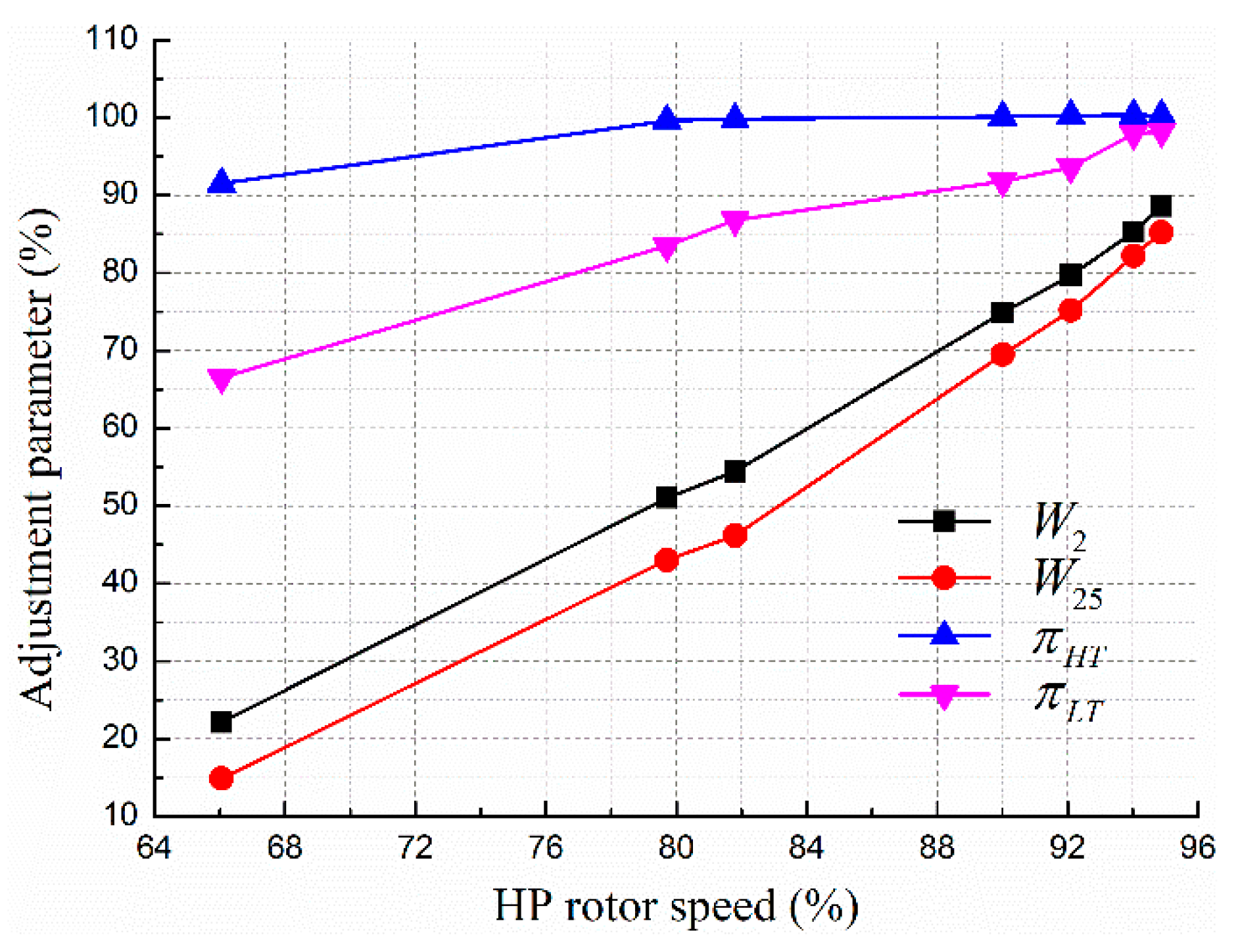
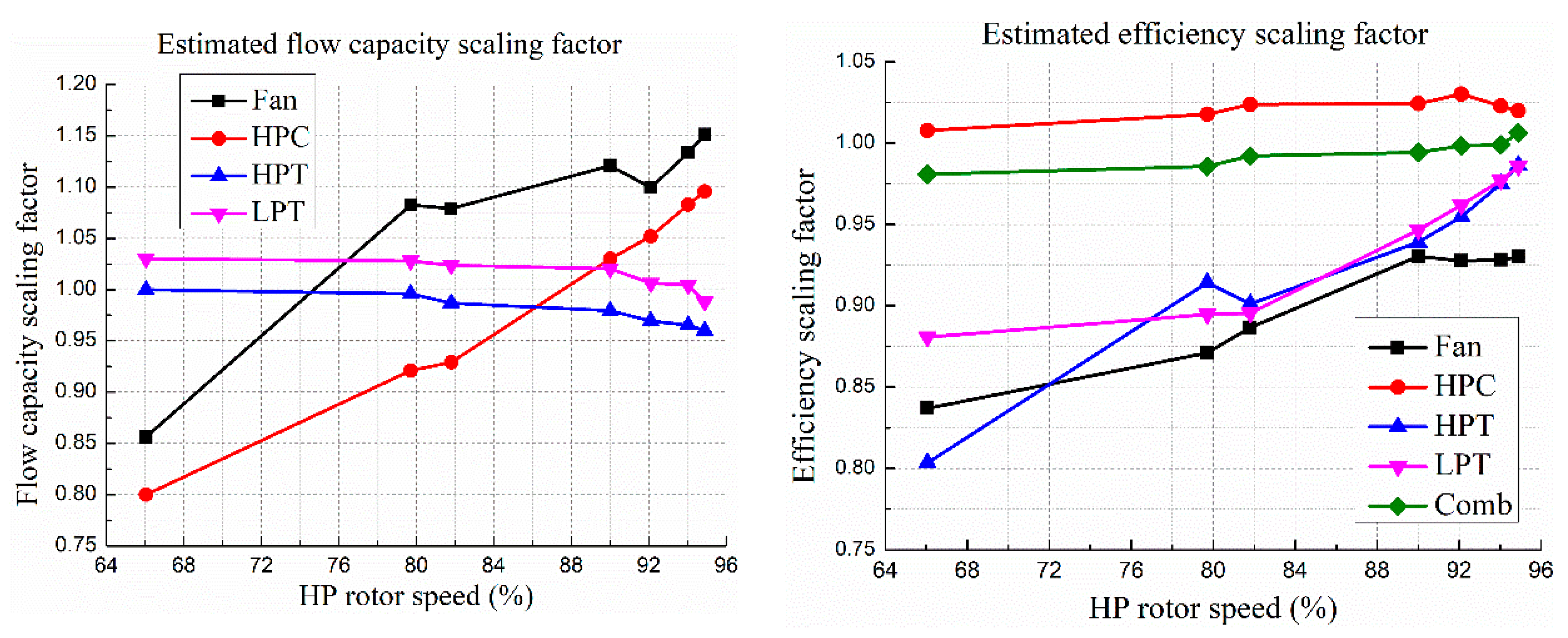
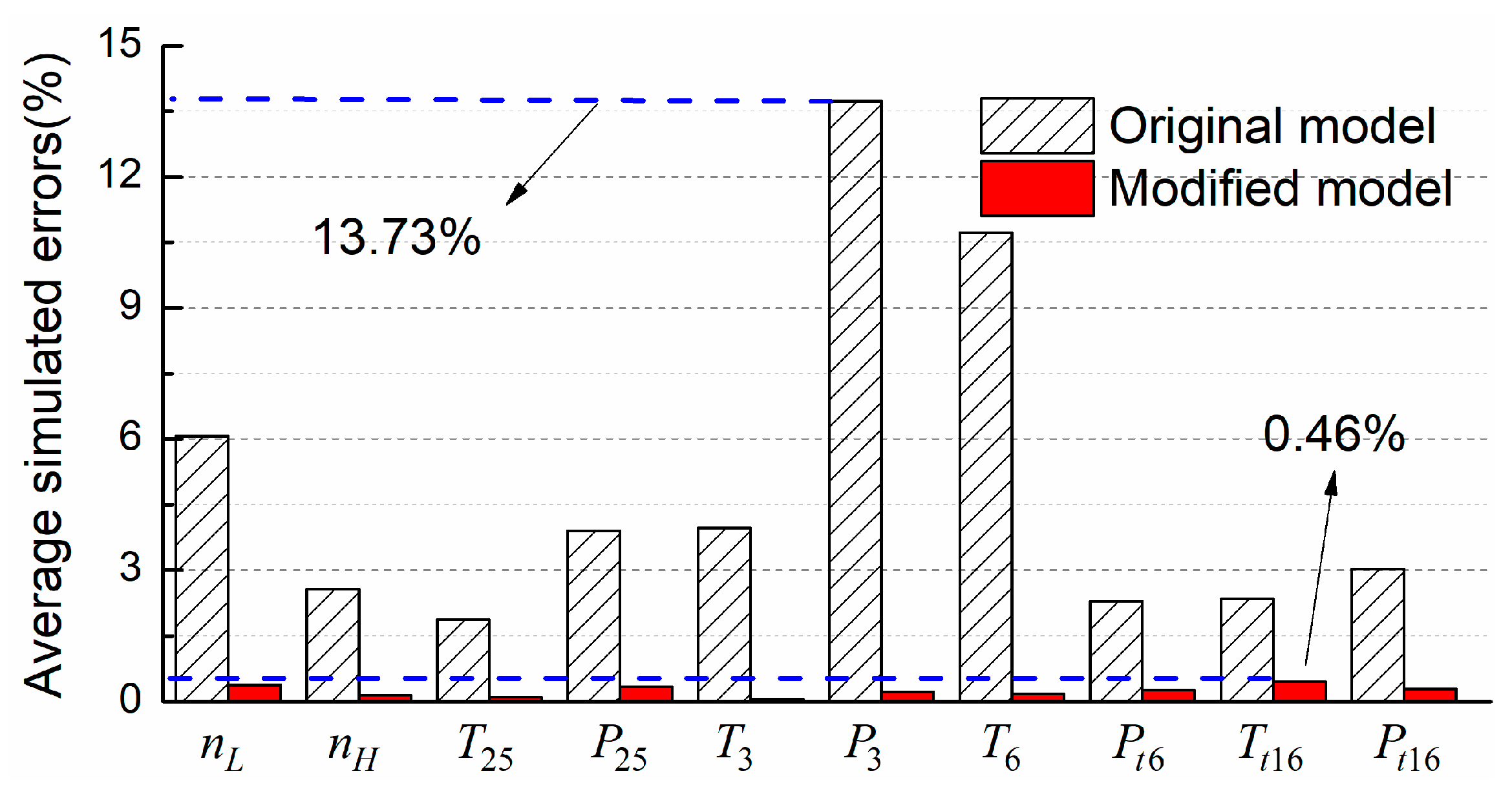
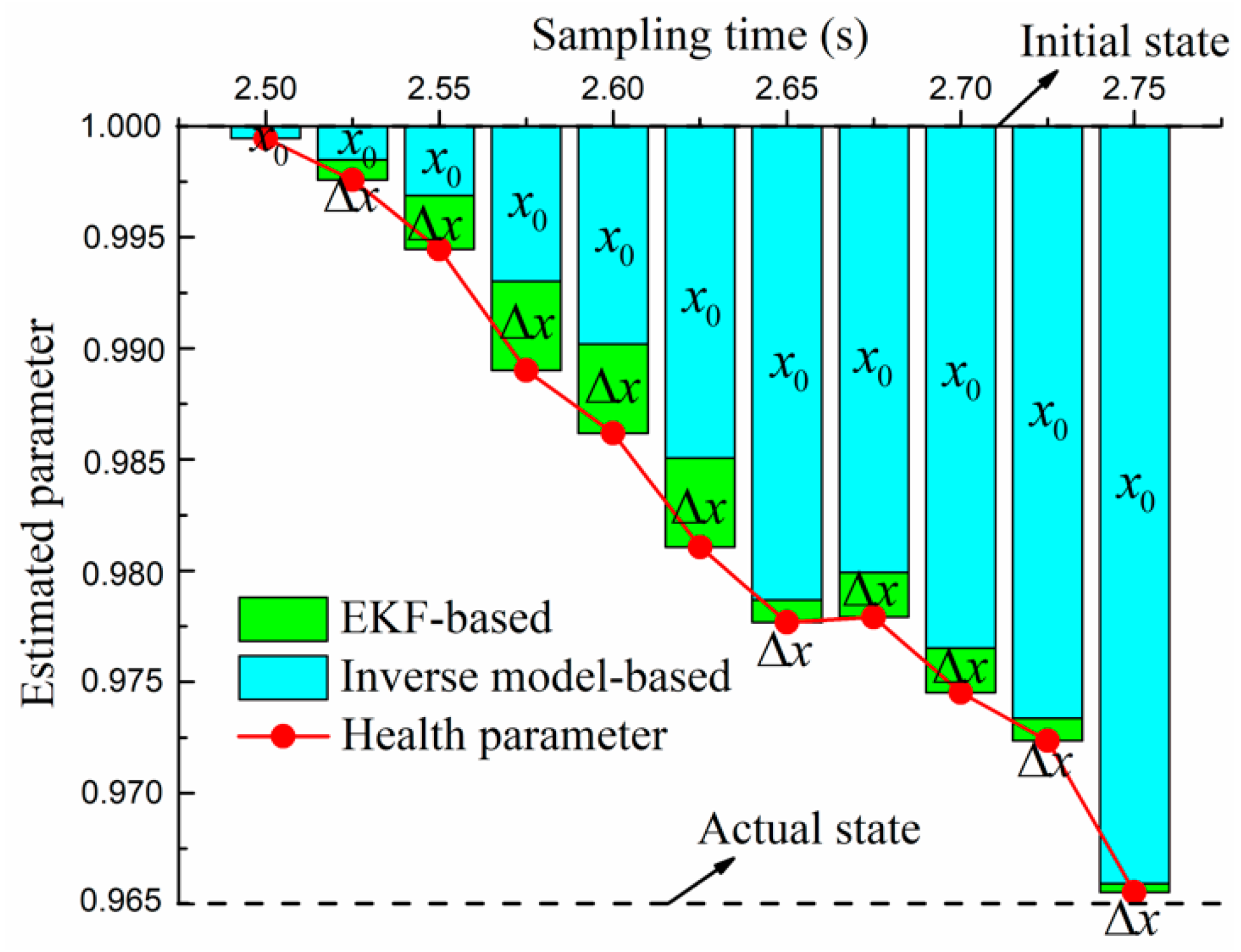
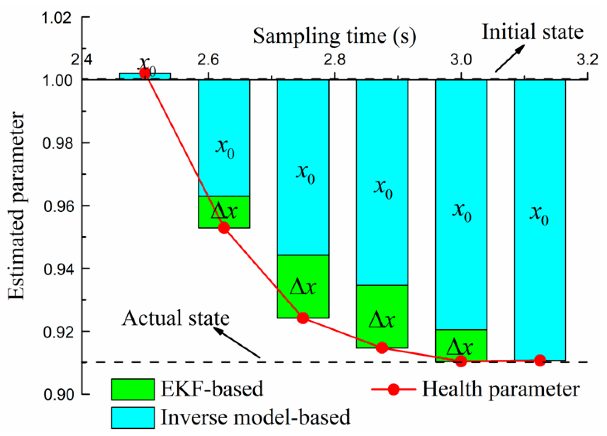
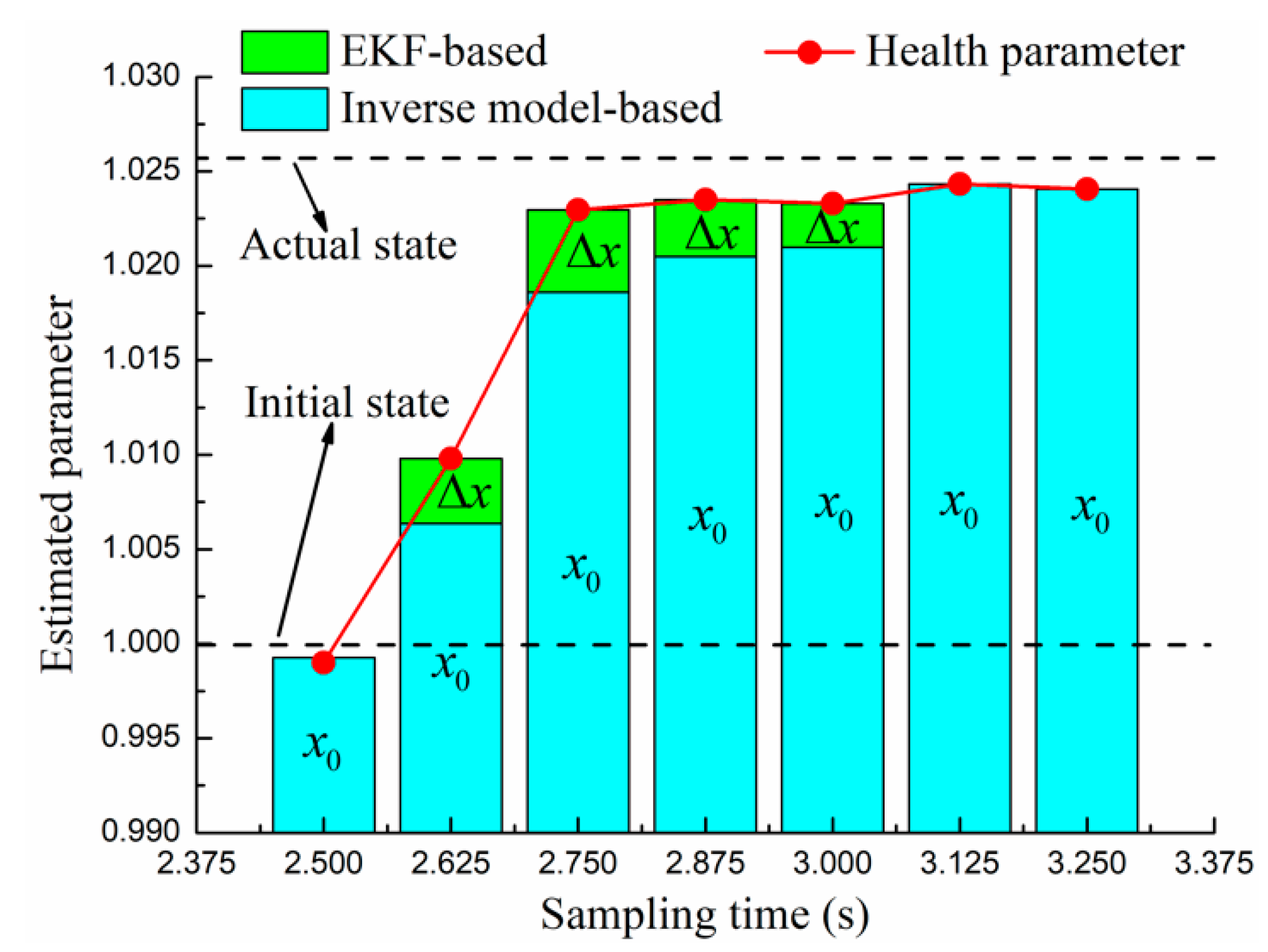
The quest to solve above problems is divided into two steps. The first step develops a new model adaptation method with respect to the twin-spool turbofan engine, which aims to improve the accuracy of the on-board engine model under steady-state conditions. AIMs of components are established to calculate the characteristic scaling factors. Considering the measurement correction, adjustment parameters are solved iteratively through the numerical solution for the engine aerodynamic matching and the accuracy improvement. The second step is an extension of the application of AIM on the performance diagnosis. The estimation dimensionality is reduced for unbiased estimation due to missing sensors between the HPT and the LPT. The theory of the rotor dynamics and modifications are integrated into the model adaptation system for the real-time gas path fault diagnosis under transient conditions. Based on the health parameters estimated from AIM, an auxiliary strategy is designed where the EKF is used for the estimation compensation to minimize the measurement residuals. With this in hand, a novel performance adaptation and diagnostic method for aero-engines based on AIM is proposed.

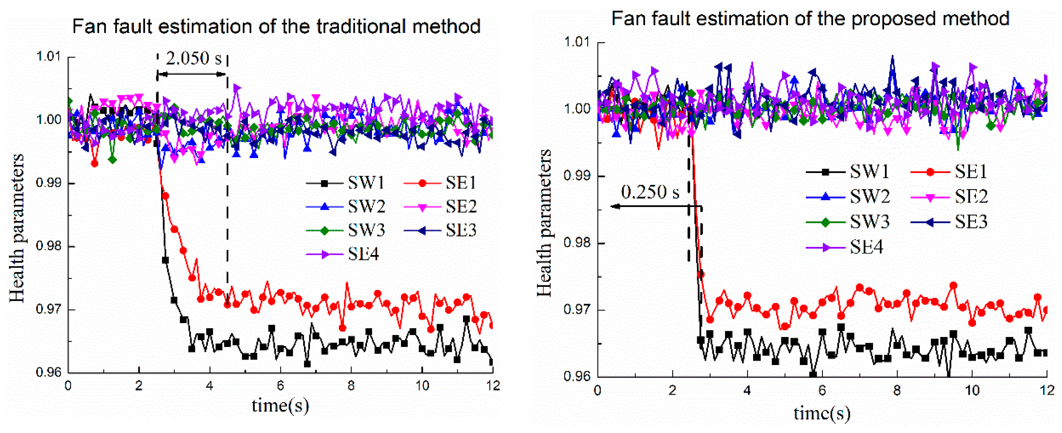
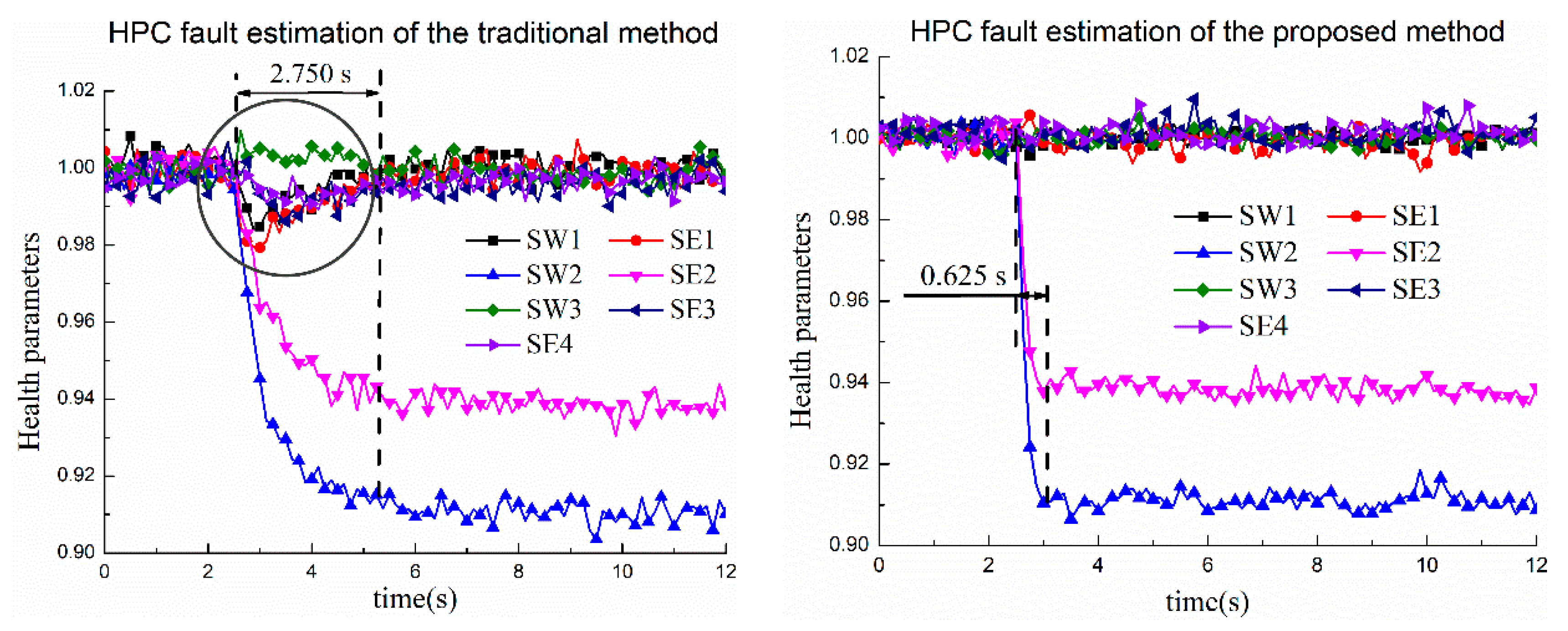
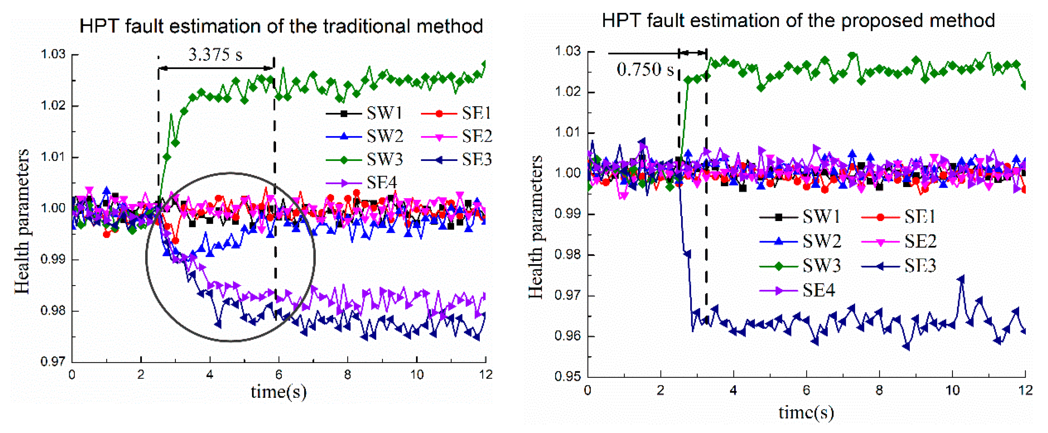
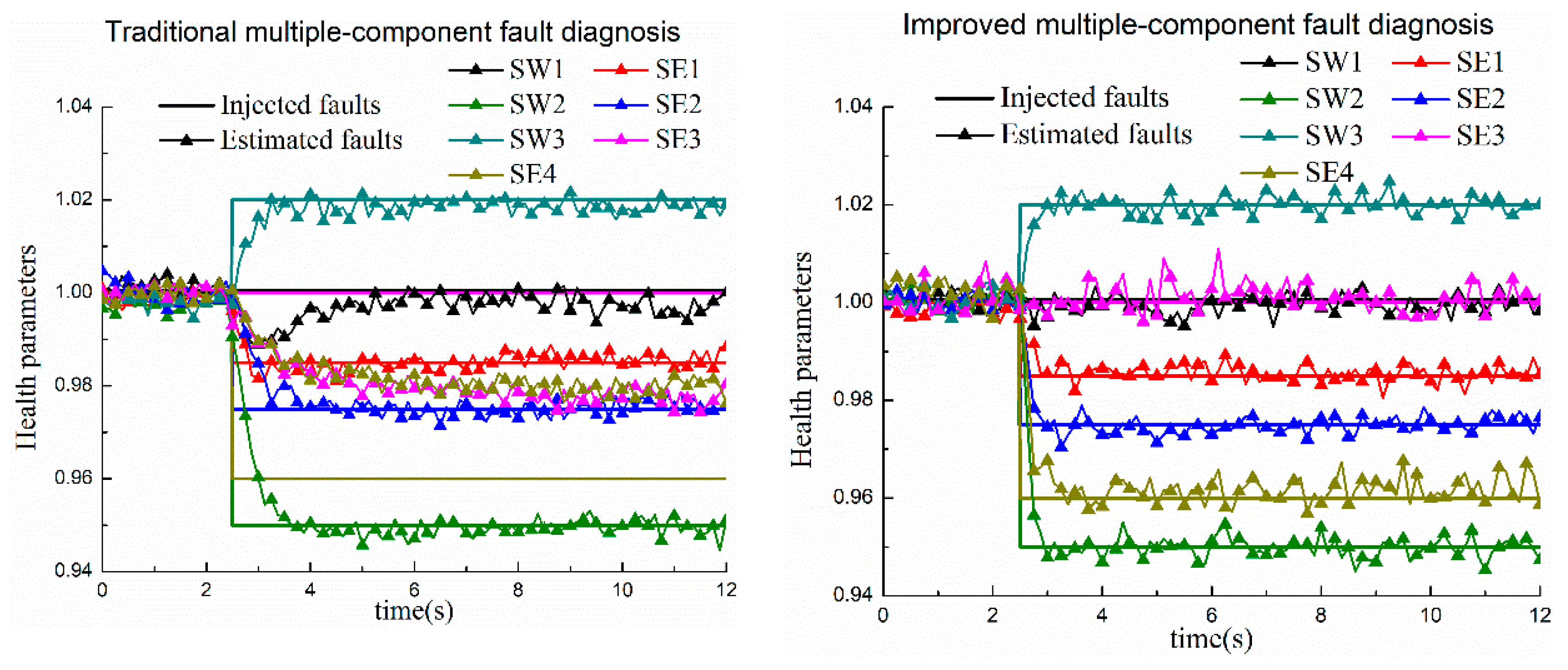
A series of simulation cases demonstrate that scaling factors can be obtained to modify the engine model to match the experimental data in the model adaptation system. In addition, under the circumstances of the single-component and multiple-component abrupt malfunction, the proposed method can achieve an unbiased estimation with fast convergence and significant accuracy improvement compared against the traditional EKF-based diagnostic method. The tests demonstrate that the proposed method exhibits the effective capacity of adaptation and diagnosis for aero-engines.

References

1. Kurz, R.; Brun, K.; Wollie, M. Degradation effects on industrial gas turbines. J. Eng. Gas Turbines Power 2009, 131, 062401. [Google Scholar] [CrossRef]
2. Fentaye, A.D.; Gilani SI, U.H.; Baheta, A.T. Gas turbine gas path diagnostics: A review. MATEC Web Conf. 2016, 74, 00005. [Google Scholar] [CrossRef]
3. Frank, P.M. Analytical and qualitative model-based fault diagnosis: A survey and some new results. Eur. J. Control 1996, 2, 6–28. [Google Scholar] [CrossRef]
4. Ghorbanian, K.; Gholamrezaei, M. An artificial neural network approach to compressor performance prediction. Appl. Energy 2009, 86, 1210–1221. [Google Scholar] [CrossRef]
5. Khustochka, O.; Yepifanov, S.; Zelenskyi, R.; Przysowa, R. Estimation of performance parameters of turbine engine components using experimental data in parametric uncertainty conditions. Aerospace 2020, 7, 6. [Google Scholar] [CrossRef] [Green Version]
6. Yang, X.; Liu, H.; Dong, K. A new component map generation method of aero engine based on experimental data. Aeronaut. Comput. Tech. 2009, 39, 48–51. [Google Scholar]
7. Khumprom, P.; Grewell, D.; Yodo, N. Deep Neural Network Feature Selection Approaches for Data-Driven Prognostic Model of Aircraft Engines. Aerospace 2020, 7, 132. [Google Scholar] [CrossRef]
8. Stamatis, A.; Mathioudakis, K.; Papailiou, K.D. Adaptive simulation of gas turbine performance. J. Eng. Gas Turbines Power 1990, 112, 168–175. [Google Scholar] [CrossRef]
9. Kong, C.; Ki, J.; Kang, M. A new scaling method for component maps of gas turbine using system identification. J. Eng. Gas Turbines Power 2003, 125, 979–985. [Google Scholar] [CrossRef]
10. Kong, C.; Kho, S.; Ki, J. Component Map Generation of a Gas Turbine Using Genetic Algorithms. J. Eng. Gas Turbines Power 2004, 128, 92–96. [Google Scholar] [CrossRef]
11. Li, Y.G.; Ghafir, M.F.A.; Wang, L.; Singh, R.; Huang, K.; Feng, X. Non-Linear Multiple Points Gas Turbine Off-Design Performance Adaptation Using a Genetic Algorithm. J. Eng. Gas Turbines Power 2010, 133, 521–532. [Google Scholar]
12. Tsoutsanis, E.; Meskin, N.; Benammar, M.; Khorasani, K. An Efficient Component Map Generation Method for Prediction of Gas turbine Performance. In Proceedings of the ASME Turbo Expo 2014: Turbine Technical Conference and Exposition, Düsseldorf, Germany, 16–20 June 2014; p. 45752. [Google Scholar]
13. Tsoutsanis, E.; Meskin, N.; Benammar, M.; Khorasani, K. A component map tuning method for performance prediction and diagnostics of gas turbine compressors. Appl. Energy 2014, 135, 572–585. [Google Scholar] [CrossRef] [Green Version]
14. Urban, L.A. Gas Path Analysis Applied to Turbine Engine Condition Monitoring. J. Aircr. 1973, 10, 400–406. [Google Scholar] [CrossRef]
15. Doel, D.L. TEMPER-A gas path analysis tool for commercial jet engines. J. Eng. Gas Turbines Power 1994, 116, 82–89. [Google Scholar] [CrossRef]
16. Pratt & Whintey. Module Analysis Program Network (Mapnet) Training Guide; Pratt & Whintey Customer Training Center: East Hartford, CT, USA, 1997. [Google Scholar]
17. Bai, J.; Fan, Z.; Sun, C. Consistence criterion for engine fault diagnosis decision. In Proceedings of the Third Asian-Pacific Conference on Aerospace Technology and Science, Kunming, China, 4–8 October 2000; pp. 407–413. [Google Scholar]
18. Brotherton, T.; Volponi, A.; Luppold, R.; Simon, D.L. eSTORM: Enhanced Self Tuning On-board Real-time Engine Model. In Proceedings of the 2003 IEEE Aerospace Conference, Big Sky, MT, USA, 8–15 March 2003; p. 1023. [Google Scholar]
19. Simon, D.L. Kalman filtering with inequality constraints for turbofan engine health estimation. Iee Proc. Control Theory Appl. 2007, 153, 371–378. [Google Scholar] [CrossRef] [Green Version]
20. Simon, D.; Simon, D.L. Constrained Kalman filtering via density function truncation for turbofan engine health estimation. Int. J. Syst. Sci. 2010, 41, 159–171. [Google Scholar] [CrossRef]
21. Ljung, L. Asymptotic Behavior of the Extended Kalman Filter as a Parameter Estimation for Linear Systems. IEEE Trans. Autom. Control 1979, 24, 36–50. [Google Scholar] [CrossRef] [Green Version]
22. Kandepu, R.; Foss, B.; Imsland, L. Applying the unscented Kalman filter for nonlinear state estimation. J. Process Control 2008, 18, 753–768. [Google Scholar] [CrossRef]
23. Arasaratnam, I.; Haykin, S. Cubature Kalman Filters. IEEE Trans. Autom. Control 2009, 54, 1254–1269. [Google Scholar] [CrossRef] [Green Version]
24. Simon, D. A comparison of filtering approaches for aircraft engine health estimation. Aerosp. Sci. Technol. 2008, 12, 276–284. [Google Scholar] [CrossRef] [Green Version]
25. Lu, F.; Ju, H.; Huang, J. An improved extended Kalman filter with inequality constraints for gas turbine engine health monitoring. Aerosp. Sci. Technol. 2016, 58, 36–47. [Google Scholar] [CrossRef]
26. Wang, C.; Huang, J.; Lu, F.; Zhou, W. Research on LPV-based model of a turbofan engine. In Proceedings of the 2015 12th International Bhurban Conference on Applied Sciences and Technology, Islamabad, Pakistan, 13–17 January 2015; IBCAST 2015. pp. 141–145. [Google Scholar]
27. Hanachi, H.; Liu, J.; Mechefske, C. Multi-mode diagnosis of a gas turbine engine using an adaptive neuro-fuzzy system. Chin. J. Aeronaut. 2018, 31, 1–9. [Google Scholar] [CrossRef]
28. Kobayashi, T.; Simon, D.L. Hybrid neural-network genetic-algorithm technique for aircraft engine performance diagnostics. J. Propuls. Power 2005, 21, 751–758. [Google Scholar] [CrossRef]
29. Dewallef, P.; Romessis, C.; LéOnard, O.; Mathioudakis, K. Combining Classification Techniques with Kalman Filters for Aircraft Engine Diagnostics. J. Eng. Gas Turbines Power 2006, 128, 595–603. [Google Scholar] [CrossRef] [Green Version]
30. Yang, C.; Kong, X.; Wang, X. Model-based fault diagnosis for performance degradations of turbofan gas path via optimal robust residuals. In Proceedings of the ASME Turbo Expo 2016: Turbomachinery Technical Conference and Exposition, Seoul, Korea, 13–17 June 2016; p. V006T05A004. [Google Scholar]
31. Li, Y.G. Performance-analysis-based gas turbine diagnostics: A review. Proc. Inst. Mech. Eng. Part A J. Power Energy 2002, 216, 363–377. [Google Scholar] [CrossRef] [Green Version]
32. Volponi, A.J. Sensor error compensation in engine performance diagnostics. In Proceedings of the ASME 1994 International Gas Turbine and Aeroengine Congress and Exposition, the Hague, The Netherlands, 13–16 June 1994; p. 78873. [Google Scholar]
33. Zhou, X.; Lu, F.; Huang, J.Q. Fault diagnosis based on measurement reconstruction of HPT exit pressure for turbofan engine. Chin. J. Aeronaut. 2019, 32, 1156–1170. [Google Scholar] [CrossRef]
34. Litt, J.S.; Parker, K.J.; Chatterjee, S. Adaptive Gas Turbine Engine Control for Deterioration Compensation due to Aging. Technical Report TM 2003-212607; NASA Glenn: Lewis, OH, USA, 2003. [Google Scholar]
35. Tsoutsanis, E.; Meskin, N.; Benammar, M.; Khorasani, K. Transient Gas Turbine Performance Diagnostics through Nonlinear Adaptation of Compressor and Turbine Maps. J. Eng. Gas Turbines Power 2015, 137, 091201. [Google Scholar] [CrossRef]
36. Sellers, J.F.; Daniele, C.J. DYNGEN: A Program for Calculating Steady-State and Transient Performance of Turbojet and Turbofan Engines; NASA-TN-D-7901; National Aeronautics and Space Administration: Washington, DC, USA, 1975. [Google Scholar]
37. Wang, X.; Chen, Z.; Yuan, Z. Nonlinear tracking-differentiator with high speed in whole course. Control Theory Appl. 2003, 20, 214–222. [Google Scholar]
38. Zhou, W.; Huang, J.; Dou, J.; Shen, F. Object-oriented simulation platform for turbofan engine and its control system. J. Aerosp. Power 2007, 22, 119–125. (In Chinese) [Google Scholar]
Figure 1. The configuration of the turbofan engine.
Aerospace 09 00016 g001
Figure 2. Compressor component inverse calculation.
Aerospace 09 00016 g002
Figure 3. Combustor inverse calculation.
Aerospace 09 00016 g003
Figure 4. Turbine component inverse calculation.
Aerospace 09 00016 g004
Figure 5. The calculation process of scaling factors.
Aerospace 09 00016 g005
Figure 6. Completed process of performance diagnosis.
Aerospace 09 00016 g006
Figure 7. The distribution diagram of estimated degradation.
Aerospace 09 00016 g007
Figure 8. Adjustment parameters in the model adaptation.
Aerospace 09 00016 g008
Figure 9. Estimated characteristic scaling factor.
Aerospace 09 00016 g009
Figure 10. Average simulated errors before and after model adaptation.
Aerospace 09 00016 g010
Figure 11. The comparison of the traditional and the proposed methods in Case 1.
Aerospace 09 00016 g011
Figure 12. The comparison of the traditional and the proposed methods in Case 2.
Aerospace 09 00016 g012
Figure 13. The comparison of the traditional and the proposed methods in Case 3.
Aerospace 09 00016 g013
Figure 14. The local analysis of SW1 in Case 1.
Aerospace 09 00016 g014
Figure 15. The local analysis of SW2 in Case 2.
Aerospace 09 00016 g015
Figure 16. The local analysis of SW3 in Case 3.
Aerospace 09 00016 g016
Figure 17. Comparison of the traditional and improved methods for multiple-component fault diagnosis.
Aerospace 09 00016 g017