Article

Assessing Baseline Carbon Stocks for Forest Transitions: A Case Study of Agroforestry Restoration from Hawaiʻi

1
Department of Natural Resources and Environmental Management, University of Hawaiʻi at Mānoa, Honolulu, HI 96822, USA
2
Heʻeia National Estuarine Research Reserve, Kāneʻohe, HI 96744, USA
3
University of Hawaiʻi Economic Research Organization, University of Hawaiʻi at Mānoa, Honolulu, HI 96822, USA
4
Water Resources Research Center, University of Hawaiʻi at Mānoa, Honolulu, HI 96822, USA
5
School of Life Sciences, University of Hawaiʻi at Mānoa, Honolulu, HI 96822, USA
6
Hawaiʻi Institute of Marine Biology, University of Hawaiʻi at Mānoa, Honolulu, HI 96822, USA
7
Kākoʻo ʻŌiwi, Heʻeia, HI 96744, USA
8
Pacific Bioscience Research Center, University of Hawaiʻi at Mānoa, Honolulu, HI 96822, USA
*
Author to whom correspondence should be addressed.
Submission received: 1 December 2020 / Revised: 12 February 2021 / Accepted: 19 February 2021 / Published: 25 February 2021

Abstract

:
As the extent of secondary forests continues to expand throughout the tropics, there is a growing need to better understand the ecosystem services, including carbon (C) storage provided by these ecosystems. Despite their spatial extent, there are limited data on how the ecosystem services provided by secondary forest may be enhanced through the restoration of both ecological and agroecological functions in these systems. This study quantifies the above- and below-ground C stocks in a non-native secondary forest in Hawaiʻi where a community-based non-profit seeks to restore a multi-strata agroforestry system for cultural and ecological benefits. For soil C, we use the equivalent soil mass method both to estimate stocks and examine spatial heterogeneity at high resolution (eg. sub 5 m) to define a method and sampling design that can be replicated to track changes in C stocks on-site and elsewhere. The assessed total ecosystem C was ~388.5 Mg C/ha. Carbon stock was highest in trees (~192.4 Mg C/ha; ~50% of total C); followed by soil (~136.4 Mg C/ha; ~35% of total C); roots (~52.7 Mg C/ha; ~14% of total C); and was lowest in coarse woody debris (~4.7 Mg C/ha; ~1% of total C) and litter (~2.3 Mg C/ha; <1% of total C). This work provides a baseline carbon assessment prior to agroforest restoration that will help to better quantify the contributions of secondary forest transitions and restoration efforts to state climate policy. In addition to the role of C sequestration in climate mitigation, we also highlight soil C as a critical metric of hybrid, people-centered restoration success given the role of soil organic matter in the production of a suite of on- and off-site ecosystem services closely linked to local sustainable development goals.

1. Introduction

Secondary forests account for over 40% of existing tropical forest cover [1] and they are projected to dominate tropical landscapes into the future [2,3]. Secondary forests can support high biodiversity and provide other societal benefits including carbon storage, nutrient cycling, timber and non-timber forest products, cultural services, and wildlife habitat [4,5,6]. However, these benefits depend on the kind of forest transitions which occur [7,8]. In some regions, particularly on islands, where invasive species dominate successional pathways [9,10], forest transitions often lead to novel ecosystems [11,12,13]. Novel ecosystems generally have relatively low native biodiversity but still can provide important ecosystem services [14,15,16]. Conservation and community-based efforts increasingly seek to improve the ecosystem services provided by these non-native, secondary forests through ecological restoration and hybrid approaches using a mix of native and non-native economic, cultural, and/or agricultural species [16,17,18]. In this context, it is critical to understand the current benefits these systems provide and how they change with management interventions.
In Hawaiʻi, non-native, secondary forest occupies 2200 km2, or 40% of total forest cover, through post-commercial-agricultural succession and invasion into formerly native-dominated vegetation [19,20] as well as into forests formerly managed through Indigenous agroecology, including Indigenous agroforestry [21,22]. These forests have little conservation value, and threaten adjacent, native forest areas through the dispersal of non-native species, and negatively impact the biocultural value of landscapes [23,24,25,26,27]. Given the relatively low conservation, economic, or cultural value of these systems, limited natural resource conservation funding in Hawaiʻi has largely focused on protecting remaining native forest or restoring forest in higher elevation pastures [28,29,30]. However, there is increasing interest in targeting non-native, secondary forest for mixed systems of ecological restoration, including integrated forest-agricultural systems or agroforestry, especially as these sites are often in more accessible, lower elevation areas [17]. Assessing the impact of restoration approaches such as agroforestry requires the development of methods to adequately evaluate the change in ecosystem services and benefits over time as well as establishing baselines that characterize ecosystem services and other benefits currently provided by these secondary forests.
Agroforestry systems span a range of practices integrating trees and crops or other tended and harvested products and are gaining traction as an effective and equitable restoration strategy [17], including in the context of the Paris Climate Accord and other climate mitigation efforts [31]. Agroforestry has been practiced by Indigenous people for millennia [32,33,34], including on Pacific Islands where they are important sources of food and other plant production while also contributing to the conservation of native biodiversity and social-ecological resilience [35,36]. In Hawaiʻi, several forms of agroforestry, adapted to a broad range of conditions [36], alongside other forms of Indigenous agriculture, were found to have to have had the potential to produce enough food for >1 million people (similar to current population levels) at the turn of the 19th century [22]. While few agroforestry systems remain today in Hawaiʻi, there is great interest in their restoration to achieve multiple benefits including local food production, biodiversity, C storage, and cultural value [17,37,38,39,40], particularly as Hawaiʻi seeks to reach carbon neutrality by 2045 while simultaneously achieving a suite of other local sustainable development goals [41].
Several recent global meta-analyses have found clear evidence that agroforestry systems generally have higher soil C [42,43] and above-ground C [44,45] compared to conventional agriculture. In contrast, in aggregate, agroforestry systems generally have lower soil C compared to paired natural forests [42,43,46]. However, Chaterjee et al. [43] disaggregated this data by agroforestry system type and found a noted exception in lowland humid tropic multi-strata agroforestry systems, which stored similar to more soil C in the top 100 cm compared with paired natural forests. This was attributed to multi-strata systems mimicking natural forests and having equal or greater root litter C from understory and overstory species compared to forests [46,47,48]. While there has been no study comparing non-native secondary forests to multi-strata agroforests, existing evidence suggests multi-strata agroforests can have as much or more soil C than natural forests [43], and that multi-strata agroforest restoration of secondary forests may have the potential to increase soil C over time, but assessing this change requires a careful methodological design.
In this study, we quantified the current carbon storage in a lowland secondary, novel forest system with low biodiversity (three dominant tree species; all non-native), where a community-based non-profit is working to restore a biodiverse and culturally valuable multi-strata agroforestry system within the Heʻeia National Estuarine Research Reserve (NERR) [17,49]. The Heʻeia NERR is the first NERR established with the explicit goal of understanding the impact of biocultural restoration on ecosystem services, including C sequestration [49]. We carried out this baseline with the explicit goal of characterizing the spatial heterogeneity of soil C in order to accurately assess the current C stock of a secondary forest as well as to determine the required sample size to quantify changes in C over time as agroforestry restoration occurs. In contrast to the majority of studies on agroforestry land-use transitions, and of land-use change in general [47,48,50,51,52], our methodology focuses on characterizing both the horizontal and vertical heterogeneity of soil C concentration and stocks at very fine scale (i.e., meter to sub-meter). In line with calls to better understand C storage in agroecological systems [53,54,55,56], we use the equivalent soil mass (ESM) method [57] as a mass-based alternative to more prevalent bulk density (volumetric) dependent methods, which reduces problems of compaction related influences on C stock measurements [58,59,60]. We discuss results in terms of implications of future sampling design to characterize change in C storage, as well as the potential for soil C to also provide an indicator for a suite of on-and off-site benefits related to healthy soils and sustainable social-ecological systems.

2. Materials and Methods
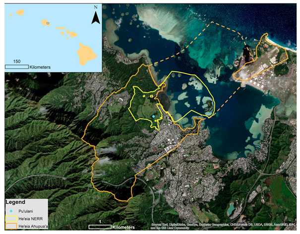
2.1. Study Site

Our study site was within the ahupuaʻa (an Indigenous social-ecological community; [61] of Heʻeia where several community-based non-profit organizations collaborate to restore Native Hawaiian land management practices including wetland taro (loʻi kalo, Colocasia esculenta), loko iʻa (traditional fish pond aquaculture), and more recently upland agroforestry systems (Figure 1) [17,49,62]. In 2017, part of the ahupuaʻa was designated as the Heʻeia National Estuarine Research Reserve (NERR) and is the first NERR specifically focusing on the restoration of social-ecological systems [49]. One of the primary goals of the NERR is to understand the potential of biocultural restoration to restore multiple ecosystem services [49]. Biocultural restoration refers to the mutually reinforcing restoration of land and culture [38,63,64].
We focused on an area within the Heʻeia NERR that is managed by the community-based non-profit Kākoʻo ʻŌiwi, whose mission is to perpetuate the cultural and spiritual practices of Native Hawaiians. In collaboration with the University of Hawaiʻi at Mānoa, a ~4000 m2 restoration area named Puʻulani (“heavenly ridge”) was selected as the first site of agroforestry restoration and a pilot to develop management and monitoring protocols [17]. Puʻulani is a sloped ridge (25–30°), located 160 m above-sea-level with a mean annual rainfall of 1370 mm [65]. Over time, Kākoʻo ʻŌiwi seeks to restore the entire ridge and a large upland area of over 80 ha of non-native forest to agroforest and native forest. At the time of sampling, Puʻulani was composed of 100% non-native tree cover, dominated by Java plum (Syzygium cumini) with some fiddlewood (Citharexylum spinosum) and octopus tree (Schefflera actinophylla). The forest understory consisted primarily of bare-ground (leaf litter), basket grass (Oplismenus hirtellus), hilo grass (Paspalum conjugatum), and maile pilau (Paederia foetida) (Figure 2a). The future vision of the site as an ecologically, culturally, and economically valuable agroforest is depicted in Figure 2b. Plants in the future restored scenario includes overstory and mid-story species: koa (Acacia koa), pualoalo (Hibiscus arnottianus), loulu (Prichardia spp.), aʻaliʻi (Dodonaea vicosa), iholena lele (Musa spp.) a Hawaiian variety of banana as well as a variety of understory species including ilieʻe (Plumbago zeylanica), pohinahina (Vitex rotundifolia), nanea (Vigna mariana), ahuʻawa (Cyprus javanicus), and kupukupu (Nepfrolepis cordifolia) [see Hastings et al. [17] for a full description of restoration plan). The soils are classified as Ultisols (Lolekaʻa silty clay; LoB), though onsite soil classifications have not been done. Three 15 m × 12 m restoration plots (spaced 5 m apart), and expanding ~760 m2 of the ridge composed the focal area of this study.

2.2. Carbon Stock Measurement and Analysis

2.2.1. Vegetation Carbon

We quantified vegetation C following standard methods for trees, roots, coarse woody debris (CWD) and litter [19,66]. All trees within each plot were identified by species and measured for diameter at breast height. We used the generalized tropical forest allometric equation for above-ground biomass (AGB; Mg C/ha) [66]:
AGB = exp[−1.803 − 0.976E + 0.976ln(ρ) + 2.673 ln(D) − 0.0299 [ln(D)]2]
where, D = diameter at breast height (DBH; cm); ρ = wood density (g/cm3), and E = a measure of environmental stress that increases with temperature seasonality, which corresponds to the duration of time a plant is exposed to stressful temperatures. A global gridded layer of E at 2.5 arc sec resolution was used from: http://chave.ups-tlse.fr/pantropical_allometry.htm (accessed on 25 February 2021). Wood density values were obtained from the tree functional attributes and ecological data base (http://db.worldagroforestry.org/ (accessed on 25 February 2021)). We estimated below-ground coarse and fine root biomass as a function of above-ground biomass following Mokany et al. (2006) and as used in a study on Hawaiʻi Island [19,67]:
y = 0.489x0.890
where, y is total root biomass and x is total above-ground biomass.
CWD, including standing or fallen dead wood >2 cm in diameter was measured [68]. We established four evenly spaced 15 m transects running down the slope within each plot, for a total of 12 transects. Along each transect, we measured the diameter of each CWD >2 cm which intersected the transect and classified it as fallen (at an <45° angle with the ground) or standing (>45° angle with the ground) debris >2 cm, which intersected the transect. There was only one piece of standing woody debris across all transects so we combined this one measurement with the fallen debris. The volume of the CWD for each transect was then calculated as:
V = π 2   d 2 / 8 × L
where d = diameter (cm) of CWD where it intersects the transect, and L = length (m) of the transect.
To calculate CWD biomass from the volume each observed CWD was assigned a decay class of 1–4 (from solid fresh wood to rotten and friable wood) following Iwashita et al. [68], which quantified the wood density (ranging from 0.69–0.07) in similar conditions in Hawaiʻi. CWD biomass was then estimated as the product of CWD volume and the associated decay class-specific wood density. To estimate CWD C content from CWD biomass, CWD biomass was multiplied by the decay-specific% C estimates from Iwashita et al. [68] for each decay class (ranging from 46.3–47.7% C). The mean C (Mg C/ha) in CWD per plot was then calculated as the mean of the 4 transects.
Litter samples were collected in six-0.25 m2 subplots randomly located within each plot. All litter within the subplot was collected and dried for 48 h at 65° to calculate the dry weight. Litter biomass was assumed to be 48% C [19].

2.2.2. Soil Carbon

To characterize the spatial heterogeneity of soil C, sixteen evenly spaced cores 3.75 m × 3.0 m apart were sampled using a grid within each 15 m × 12 m plot for a total of 48 soil cores over the three plots. Cores were sampled at five, 20 cm increments to a depth of 1 m. Each of the 20 cm increment samples were homogenized (mixed thoroughly) in the field post-extraction and the wet mass recorded. In the laboratory, soil samples were passed through a 2 mm sieve to remove all larger roots and rocks. Subsamples were oven-dried to a constant mass at 105 °C to determine moisture content, ground using a mortar and pestle, passed through a 250 µm sieve, and then analyzed for C concentration (% C) on a mass basis using an elemental analyzer (Carlo Erba Instruments NC 2500 Now Thermo Scientific, Waltham, MA, USA).

2.2.3. Carbon Stock–Equivalent Soil Mass Method

We used the Equivalent Soil Mass (ESM) method to quantify baseline soil C stock [57]. The ESM method is a mass-based approach for quantifying soil C stock using the cumulative mass of soil measured in the profile rather than the more widely used depth-based approach which relies on bulk density [69]. Land use and management directly impact bulk density and can bias comparative studies of C stocks over time or among treatments [60]. Instead, the ESM method is used to evaluate soil C stock in the context of land- use or management change [59], when processes such as compaction, tillage, and restoration of organic matter inputs are expected to change bulk density [57,60,70,71]. Curve fitting is used to develop a mathematical equation that describes the relationship between total soil mass and total carbon mass through each soil profile.
Following Wendt and Hauser [57], we fit quadratic polynomial equations to estimate the mass of C throughout each soil core. The specific reference mass used to make direct comparisons over time or between treatments is site-dependent and based on the mass of soil within each soil profile. As long as the reference mass chosen falls within the boundaries of the dataset collected for all profiles, any mass increment may be chosen for comparison and there is no limitation to the number of increments. We chose increments of 800 Mg/ha because (1) the average mass 20 cm samples across all plots was 830.3 Mg/ha, which makes the C stock roughly comparable to depth-based C stocks reported for the top 20 cm of soil and (2) all the cores had a mass of at least 4800 Mg/ha at the 1 m depth. Accordingly, we assigned the following mass increments: 800, 1600, 2400, 3200, 4000, and 4800 ESM intervals. The ESM of 4800 Mg/ha represented approximately ~80 cm of soil in this system, when averaged between the plots. We highlight both surface soil C (Mg C/ha, ESM 800) and deep soil C stock (Mg C/ha, ESM 4800) for this baseline assessment.

2.2.4. Geospatial Analysis and Kriging

Geospatial statistics have been used in soil science to quantitatively determine the spatial scales and patterns of soil characteristics, such as salinity, pollution by heavy metals, water content, nutrient content [72,73,74,75], as well as soil C following land-use change [76]. A common application of geospatial statistics is to interpolate soil properties as continuous surfaces over the landscape from point-based samples [77,78,79]. This approach relies on quantifying the spatial dependence among samples, or the relationship between the variability in sampled values and their location with respect to each other [72,80], which can then be used to infer scales of variation, or correlation ranges where observable change in soil properties can occur [74,75,77]. In addition, geospatial analysis can be used to inform subsequent spatial analysis (e.g., kriging and hybrid interpolation techniques) as well as guide future sampling [73]. The spatial dependence of soil C stock (ESM 4800) was quantified by plotting a variogram of the semivariance among pairs of sample points against the distance between them and fitting a Matérn model estimated by weighted least squares to the variogram. This relationship indicates the minimum semivariance, or nugget, which is the variance among immediately adjacent samples (i.e., due to random variation) as well as the range, which is the distance at which spatial dependence is no longer present among samples [75,81]. For our modeled variogram, we set the maximum distance between sample points to 20 m based on our plot area. This ensures the minimum number of pairs for the model and displays points for pairs of sample locations 20 m apart or less. Kriging, a form of optimum prediction, has been recognized as superior interpolation technique among many methodologies to make quantitative predictions at unsampled locations based on properties from nearby measured locations [82,83], with various applications in environmental science [75], including soil C [73,83,84,85]. The parameter estimates obtained from the variogram model fit were used in kriging operations to parameterize predictions of C values at unsampled locations within the plots [81,86]. Interpolated contour maps were produced by Bayesian kriging [86] displaying the vertical and horizontal heterogeneity of both C concentration and stock. Kriging enhanced the resolution by a factor of 15 from the original 48 cores sampled at ~20 m, and generated quantitative predictions at 752 new locations to produce interpolated contour maps at ~1.3 m resolution. These 752 values were predicted for both C concentration and C stocks (ESM 800 and ESM 4800). Contour maps were produced to characterize and display heterogeneity in soil C parameters.

3. Results

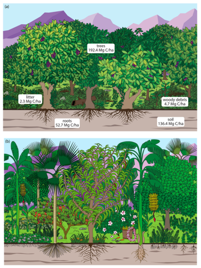
3.1. Ecosystem Carbon
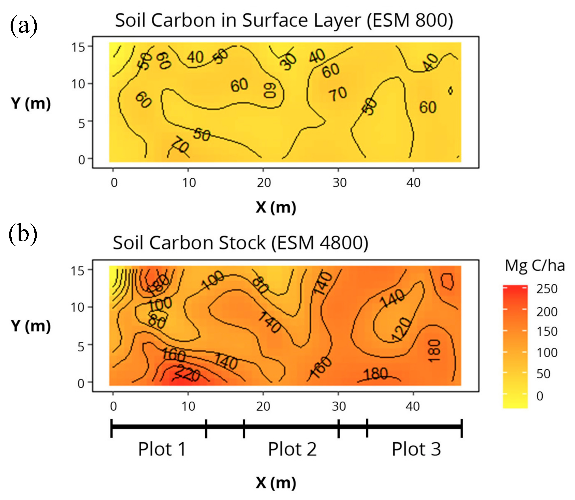
Total ecosystem C across the three plots was 388.5 ± 18.6 (Mg C/ha ± one standard error (SE)). Overall, C was highest in trees (192.4 ± 19.2 Mg C/ha; ~50% of total C); followed by soil (136.4 ± 7.9 Mg C/ha; ~35% of total C); roots (52.7 ± 4.7 Mg C/ha; ~14% of total C); and was the lowest in coarse woody debris (4.7 ± 2.8 Mg C/ha; ~1%) as well as litter (2.3 ± 0.2 Mg C/ha; <1% of total C) (Figure 2a; data available in Supplementary Information).

3.2. Soil Carbon

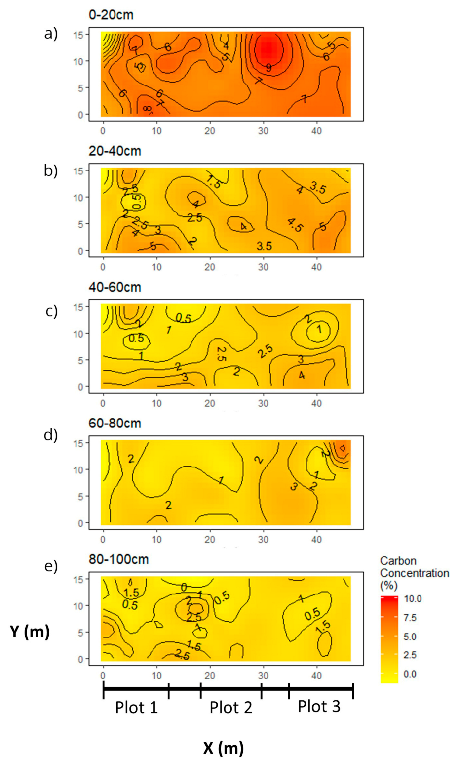
3.2.1. Percent Carbon

Mean soil C concentration decreased with depth across all plots from 6.1% C ± 0.1% C in the surface samples (0–20 cm) to 1.2% C ± 0.0% C in the deepest samples (80–100 cm; Figure 3). Contoured maps of C concentration also show a high degree of spatial heterogeneity within each depth (Figure 3a–e). For example, among surface samples (0–20 cm), C concentration varied from 1.7% C to 8.2% C with a notable area of high C concentration between plots 2 and 3 (Figure 3a).

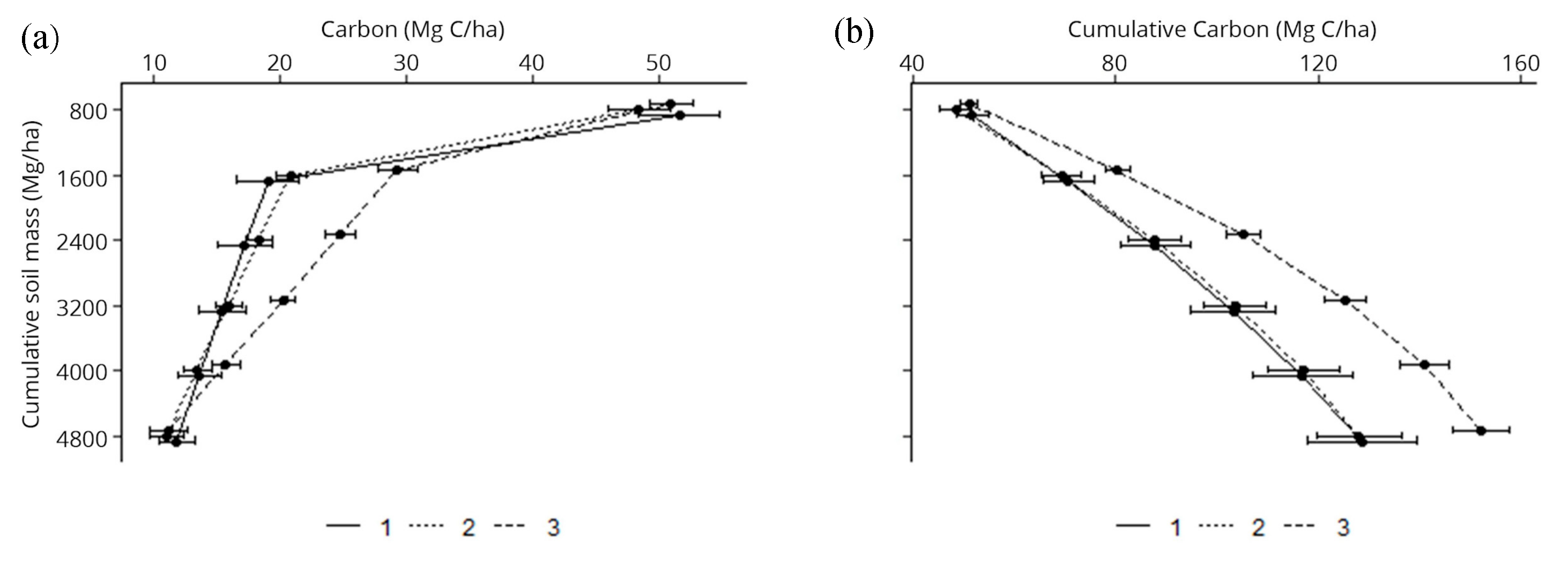
3.2.2. Total Soil Carbon Stock

Mean soil C stock in the surface layer (ESM 800; roughly corresponding to 0–20 cm) was 50.3 ± 1.0 Mg C/ha (Figure 4a). Primarily due to the rapid decline soil C concentration, the mean soil C stock also declined with each ESM increment, lowering to 11.4 ± 0.2 Mg C/ha in the ESM 4000–4800 Mg/ha increment (Figure 4a). Mean cumulative soil C stock (ESM 4800; roughly corresponding to 0–80 cm) for the three plots was 136.4 ± 7.9 Mg C/ha (Figure 4b).
The spatial variability of the surface C stock (ESM 800; Figure 5a) follows similar distribution patterns as the surface soil C concentration. Kriged interpolations of deep soil C stock (ESM 4800; Figure 5b) reveal spatial heterogeneity in some places ranging from ~80–220 Mg C/ha within 8 m.

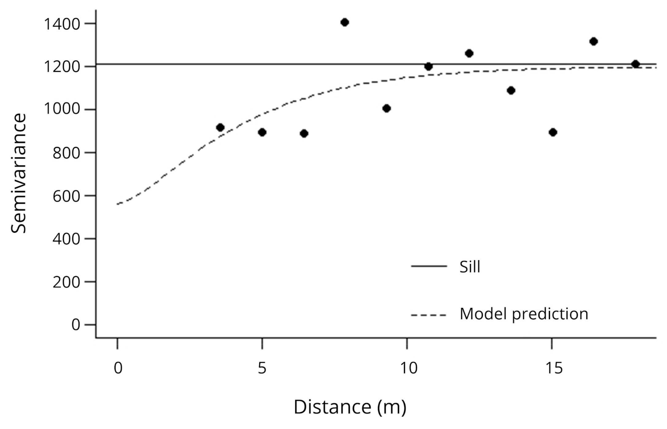
3.2.3. Spatial Dependence of Total C Stock

The computed variogram illustrates the soil C stock spatial relationships for 22 pairs of sample points (e.g., all point pairs ≤20 m apart). The range, or distance beyond which the sample values are spatially independent, is ~11.6 m, and is the location where the model prediction intersects the sill (Figure 6). The nugget, or variance among immediately adjacent samples was approximately 580 units of variance and the sill, or the maximum semivariance among samples, was approximately 1180 units of variance and is shown where the semivariogram model begins to flatten out (Figure 6). The ratio of the nugget to sill, a quantitative estimate of overall spatial dependence, was 49%, which is considered moderate for soil properties [77,87,88,89]. The 11.6 m value also can be interpreted as indicating samples collected more closely than 11.6 m are reporting similar information rather than new information.

4. Discussion

This case study provides insight on current C storage in a novel secondary forest, a prevalent but poorly understood forest type in Hawaiʻi [9,90] and other parts of the tropics [3,91,92]. Qunatifying soil C using the equivalent soil mass method as presented in this study can be applied in other areas, and the results provide insight into the spatial heterogeneity of soil C that can inform future sampling desing. We discuss key insights and lessons from the results and methodology presented in this study and also highlight the importance of soil C as a potential indicator of restoration success in the context of biocultural restoration of an agroforestry system.

4.1. Lesson 1: Accurate Carbon Stock Assessment Requires Inclusion of Both Above- and Below-Ground Carbon Pools

Results of this study demonstrate the importance of including both above-ground and below-ground C in carbon assessments, echoing calls for greater attention to soil C in carbon assessments [76,93,94]. In our study area, ~51% of ecosystem C was stored above-ground in large non-native trees (primarily Java plum; Syzygium cumini), coarse woody debris, and leaf litter, while 49% was stored below-ground in soil and roots (of which soil C accounted for 35% of total C). Above-ground C (~199.4 Mg C/ha) was over twice as high as the mean above-ground C of wet-mesic non-native forests across the state (90.9 Mg C/ha) [20], although it was within the range of non-native forest dominated by large invasive trees including Fraxinus uhdei [90]. The high above-ground C found in this study is likely due to the low elevation and large java plum (Syzygium cumini) in this system, compared with many wet-mesic non-native forests across the state which are often dominated by smaller stature invasive trees such as strawberry guava (Psidium cattleinanum) with lower carbon storage [90]. It must be emphasized that site-level biomass measurements are limited for non-native, secondary forest in Hawaiʻi [95], and thus these results contribute to our fundamental understanding of the variability inherent in these novel ecosystems.
In contrast, soil C at Puʻulani was lower than the average soil C estimates (to 100 cm) across the state in wet-mesic non-native forests (136.4 ± 7.9 Mg C/ha compared to the statewide average of 180.5 Mg C/ha [20]. Soil C found at Puʻulani is likely lower both due to the use of the ESM method, which resulted in using less than the full 100 cm sample (see discussion in 4.2) as well as to the fact that many wet-mesic non-native forests soils are Andisols, which store large amounts of soil C due to their biogeochemical properties [96,97]. However, compared with soils in the same classification in Hawaiʻi, soils at Puʻulani exhibited high C concentrations. Soils in our sampling site are classified as Ultisols (Lolekaʻa silty clay), for which the original type location data describes this soil as having 3.2% C in 0–25 cm and 0.6% C in 84–107 cm depths [98]. In comparison to the type location data, the percent C at Puʻulani was substantially higher at comparable depths (6.1% C in 0–20 cm and 1.2% C 80–100 cm respectively).

4.2. Lesson 2: The Equivalent Soil Mass Method (ESM) Provides a Practical Mass-Based Method to Characterize Soil C Stocks at Depth

Second, our results reiterate the importance of sampling at depth (~100 cm) using a quantitative method--the equivalent soil mass method (ESM)--designed specifically for assessing land-use change [57,60]. Such sampling is increasingly called for to better understand current C stocks and change with land-use transitions [53,56,76,99]. While the majority (63%) of soil C in this study was in the surface layer (ESM 800), there was a substantial portion of soil C in the subsurface soil (in the ESM increments 1600, 2400, 3200, 4000, and 4800). This is a similar magnitude to other studies which have found that globally subsurface soil (30–100 cm) contains an average of 47% of the entire soil C stock [100]. Often inadequately characterized in C studies, these deeper soil layers can hold more persistent C pools (i.e., stabilized and stored for a longer time), but can also be affected by land-use change [99,101,102,103]. Deeper sampling is becoming more common [102] as there is increasing recognition of microbial interactions that affect C storage dynamics even below a 100 cm depth [104,105]. While the ESM provides an alternative to bulk-density dependent methods which can be unreliable in the context of land-use change [57], it is important to note that it is advisable to sample to depths greater than 100 cm (or the desired depth) in order to capture the full profile as the ESM is limited by the samples with the lowest mass. In the case of this study, our last ESM (ESM 4800) constituted an average of ~80 cm depth given the lower mass of some samples.

4.3. Lesson 3: Geospatial Analysis Can Effectively Characterize Spatial Heterogeneity and Inform Future Sampling Effort

Third, we demonstrate the use of geospatial analyses to characterize the heterogeneity of C in a secondary forest system. The nugget to sill ratio of the semivariogram (Figure 6), a measure of spatial dependence, was 49% which is within the moderate range for soil properties [77,87,88,89]. From the perspective of future sampling, the range of the semivariogram in this study indicated that samples further away than ~11.6 m are spatially independent. Thus, if future sampling requires statistically independent samples to, for example, test for differences in plot-level treatments, the range indicates the minimum distance to maintain between soil samples. In contrast, for repeat robust spatial interpolation as we have performed here, a sampling interval of ~5.8 m or less (half of the semivariogram range) is recommended [106,107]. These results indicate that we could reduce future sampling intensity from a grid of n = 16 to n = 9 in each plot and still adequately interpolate the data.
The interpolated contour maps by kriging (Figure 3 and Figure 5) display both vertical and horizontal heterogeneity of soil C concentration and C stock. Surface soils (i.e., to 0–20 cm and ESM 800 respectively) not only contained the highest C concentrations and majority of C mass, but were also the most spatially heterogeneous and variable, with values ranging over an order of magnitude (Figure 3). Quantification of spatial variability of soil properties is more often conducted for large areas [73,108,109], while this study provides evidence of small-scale spatial variability of soil C and importance of fine scale sampling [110].

4.4. Lesson 4: Soil Carbon Is More Than Just the Ecosystem Service of Climate Mitigation; It Can Serve as a Holistic Indicator of Success in Biocultural Restoration of Agroforestry Systems

Over time, as our study system in Heʻeia moves from a monoculture invasive tree dominated system to a diverse and multi-strata agroforestry system (Figure 2), soil C storage may increase over the long-term, though a decline in soil C may occur in the early years of restoration due to initial clearing and planting disturbance [44]. As with a variety of diversified agricultural systems, multi-strata agroforestry systems are often designed and managed in ways that increase soil organic matter or soil C (e.g., through composting, crop rotation, perennial vegetation with greater root inputs), which in addition the ecosystem service of C sequestration, also underpins a suite of other on- and off-site ecosystem services, including increased crop yields, resilience to pests, and water retention capacity [39,53,111]. Soil C is also an indicator of soil fertility and can reduce the need for external inputs, making the system itself more self-sustaining, which is often a goal of agroforestry [42,43,53,112,113]. These ecosystem system benefits are particularly relevant for organizations like Kākoʻo ʻŌiwi and the Heʻeia NERR who seek to restore multi-functional Indigenous agricultural systems using a biocultural approach [49], which favor low external inputs and high functional and species diversity [17]. The species selected for restoration all provide important linked cultural and ecological value and rely on healthy soils to thrive. A critical metric for success is an increased connection of community to the forest [17], and soil C will be central in this vision as a critical indicator of the ability of the system to thrive and contribute to multiple local sustainable development goals, including local food production, carbon sequestration, and biodiversity protection [41].

5. Conclusions

As the area of tropical secondary forests continues to expand, so will efforts to enhance the ecosystem services provided by these systems. This case study from Hawaiʻi provides a methodology for documenting baseline C storage in a non-native secondary forest, with widespread application to other restoration projects seeking to assess this benefit alongside others cultural, ecological, and economic benefits. It also provides foundational information on C quantity and heterogeneity in an ecosystem in Hawaiʻi that is poorly studied despite its large extent across the islands. We demonstrate the importance of including both above- and below-ground carbon stocks as ~49% of ecosystem C was found below-ground (in soil and roots), including ~35% in the top ~80 cm of soil. Using the equivalent soil mass method, which provides a metric less sensitive to future land-use change, we also confirm the value of sampling beyond surface depths, as ~37% of soil C was found in subsurface (~20–80 cm) layers. Finally, we demonstrate the utility of geospatial methods to quantify the spatial heterogeneity of soil C, which can provide insight into appropriate sampling design for monitoring. As the biocultural restoration of this site continues, these results additionally suggest that soil C can be a useful indicator of soil health, which underpins a suite of on and off-site ecosystem services, thereby contributing to a range of both local and global sustainable development goals.

Supplementary Materials

The following are available online at https://0-www-mdpi-com.brum.beds.ac.uk/2077-0472/11/3/189/s1, Supplementary Information.

Author Contributions

Conceptualization, L.L.B., S.E.C., T.T., Z.H., A.M., C.T., K.K.-S.; methodology, S.E.C., L.L.B., A.M.; field work, A.M., L.L.B., M.W., Z.H., S.J.W.; lab analysis, A.M., M.W., S.E.C.; formal analysis, A.M., C.T., L.L.B., S.E.C.; writing—original draft preparation, A.M., L.L.B.; writing—review and editing, A.M., L.L.B., S.E.C., C.T., Z.H., T.T., M.W., K.K.-S., S.J.W., Y.M.R., K.B.W.; visualization, A.M., C.T., S.E.C., Y.M.R., L.L.B.; supervision, L.L.B., S.E.C., C.T., K.B.W., Y.M.R.; funding acquisition, L.L.B., T.T., C.T., K.B.W. All authors have read and agreed to the published version of the manuscript.

Funding

This research was funded in part by: (1) the Natural Resources Conservation Service, Conservation Innovation Grant #NR18925190002G003; (2) the University of Hawaiʻi Social Science Research Institute Research Support Grant; (3) Office for Coastal Management, National Ocean Service, National Oceanic and Atmospheric Administration Grant 11.420, Coastal Zone Management Estuarine Research Reserves Award ID#s NA19NOS4200078 and NA20NOS4200095; (4) grant/cooperative agreement from the National Oceanic and Atmospheric Administration, Project R/HE-38, which is sponsored by the University of Hawaii Sea Grant College Program, SOEST, under Institutional Grant No. NA18OAR4170076 from NOAA Office of Sea Grant, Department of Commerce. UNIHI-SEAGRANT-JC-20-04.; (5) the National Science Foundation EPSCoR Award No. OIA #1557349; (6) the USDA National Institute of Food and Agriculture, Hatch project # HAW1151-H, managed by the College of Tropical Agriculture and Human Resources at the University of Hawaiʻi at Mānoa; (7) and the USDA NIFA Renewable Natural Resources Extension Act; 8) NSF Graduate Research Fellowship (#1842402; Z.H). The views in this paper are the authors’ and do not necessarily reflect those of the funding organizations or sub-agencies.

Data Availability Statement

All carbon data presented is available as supplementary material.

Acknowledgments

We would like to acknowledge: Russell Yost for providing expertise on geospatial and geostatistical analysis and reporting znc Amanda Toperoff with Big Blue Animation and Design lab for generating the pre- and post-restoration depiction. We also thank Paul Selmants for assistance with above-ground carbon sampling design; Christine Tallamy-Glazer, Jon Wells, Elaine Vizka and Casey McGrath of the Crow lab for assistance sampling, laboratory, and data analysis; and Jade Delevaux, Gina McGuire, and Victoria Ward for assistance with figures. We also thank Aurora Kagawa-Viviani for her mentorship and Paul Pestana for field and laboratory assisstance. A special Mahalo (thank you) to Mahealani Botelho who co-designed the Puʻulani Project, Nick Reppun, and all staff and caretakers of Kākoʻo ʻŌiwi, the He’eia NERR, the volunteers who assisted in data collection, as well as the larger Heʻeia community. This is contributed paper CP-2021-11 of the Water Resources Research Center and publication JC-20-04 of the University of Hawaiʻi Sea Grant College Program, both at the University of Hawaiʻi at Mānoa, Honolulu, Hawaiʻi.

Conflicts of Interest

The authors declare no conflict of interest.

References

  1. Brown, S.; Lugo, A.E. Tropical Secondary Forests. J. Trop. Ecol. 1990, 6, 1–32. [Google Scholar] [CrossRef]
  2. Cortés-Calderón, S.; Mora, F.; Arreola-Villa, F.; Balvanera, P. Ecosystem Services Supply and Interactions along Secondary Tropical Dry Forests Succession. For. Ecol. Manag. 2021, 482, 118858. [Google Scholar] [CrossRef]
  3. Chazdon, R.L.; Harvey, C.A.; Komar, O.; Griffith, D.M.; Ferguson, B.G.; Martínez-Ramos, M.; Morales, H.; Nigh, R.; Soto-Pinto, L.; Breugel, M.V.; et al. Beyond Reserves: A Research Agenda for Conserving Biodiversity in Human-Modified Tropical Landscapes. Biotropica 2009, 41, 142–153. [Google Scholar] [CrossRef] [Green Version]
  4. Matos, F.A.R.; Magnago, L.F.S.; Miranda, C.A.C.; de Menezes, L.F.T.; Gastauer, M.; Safar, N.V.H.; Schaefer, C.E.G.R.; da Silva, M.P.; Simonelli, M.; Edwards, F.A.; et al. Secondary Forest Fragments Offer Important Carbon and Biodiversity Cobenefits. Glob. Chang. Biol. 2020, 26, 509–522. [Google Scholar] [CrossRef]
  5. Naime, J.; Mora, F.; Sánchez-Martínez, M.; Arreola, F.; Balvanera, P. Economic Valuation of Ecosystem Services from Secondary Tropical Forests: Trade-Offs and Implications for Policy Making. For. Ecol. Manag. 2020, 473, 118294. [Google Scholar] [CrossRef]
  6. Zeng, Y.; Gou, M.; Ouyang, S.; Chen, L.; Fang, X.; Zhao, L.; Li, J.; Peng, C.; Xiang, W. The Impact of Secondary Forest Restoration on Multiple Ecosystem Services and Their Trade-Offs. Ecol. Indic. 2019, 104, 248–258. [Google Scholar] [CrossRef]
  7. Rudel, T.K.; Coomes, O.T.; Moran, E.; Achard, F.; Angelsen, A.; Xu, J.; Lambin, E. Forest Transitions: Towards a Global Understanding of Land Use Change. Glob. Environ. Chang. 2005, 15, 23–31. [Google Scholar] [CrossRef]
  8. Wilson, S.; Schelhas, J.; Grau, R.; Nanni, A.; Sloan, S. Forest Ecosystem-Service Transitions: The Ecological Dimensions of the Forest Transition. Ecol. Soc. 2017, 22. [Google Scholar] [CrossRef] [Green Version]
  9. Hughes, R.F.; Asner, G.P.; Mascaro, J.; Uowolo, A.; Baldwin, J. Carbon Storage Landscapes of Lowland Hawaii: The Role of Native and Invasive Species through Space and Time. Ecol. Appl. 2014, 24, 716–731. [Google Scholar] [CrossRef]
  10. Guariguata, M.R.; Ostertag, R. Neotropical Secondary Forest Succession: Changes in Structural and Functional Characteristics. For. Ecol. Manag. 2001, 148, 22. [Google Scholar] [CrossRef]
  11. Hobbs, R.J.; Higgs, E.; Harris, J.A. Novel Ecosystems: Implications for Conservation and Restoration. Trends Ecol. Evol. 2009, 24, 599–605. [Google Scholar] [CrossRef] [PubMed]
  12. Hobbs, R.J.; Higgs, E.S.; Harris, J.A. Novel Ecosystems: Concept or Inconvenient Reality? A Response to Murcia et Al. Trends Ecol. Evol. 2014, 29, 645–646. [Google Scholar] [CrossRef] [PubMed]
  13. Hobbs, R.J.; Valentine, L.; Standish, R.; Jackson, S. Movers and Stayers: Novel Assemblages in Changing Environments. Trends Ecol. Evol. 2017, 33, 116–128. [Google Scholar] [CrossRef] [Green Version]
  14. Collier, M.J. Novel Ecosystems and the Emergence of Cultural Ecosystem Services. Ecosyst. Serv. 2014, 9, 166–169. [Google Scholar] [CrossRef] [Green Version]
  15. Evers, C.R.; Wardropper, C.B.; Branoff, B.; Granek, E.F.; Hirsch, S.L.; Link, T.E.; Olivero-Lora, S.; Wilson, C. The Ecosystem Services and Biodiversity of Novel Ecosystems: A Literature Review. Glob. Ecol. Conserv. 2018, 13, 13. [Google Scholar] [CrossRef]
  16. Burnett, K.M.; Ticktin, T.; Bremer, L.L.; Quazi, S.A.; Geslani, C.; Wada, C.A.; Kurashima, N.; Mandle, L.; Pascua, P.; Depraetere, T.; et al. Restoring to the Future: Environmental, Cultural, and Management Trade-Offs in Historical versus Hybrid Restoration of a Highly Modified Ecosystem. Conserv. Lett. 2019, 12, e12606. [Google Scholar] [CrossRef] [Green Version]
  17. Hastings, Z.; Ticktin, T.; Botelho, M.; Reppun, N.; Kukea-Shultz, K.; Wong, M.; Melone, A.; Bremer, L. Integrating Co-Production and Functional Trait Approaches for Inclusive and Scalable Restoration Solutions. Conserv. Sci. Pract. 2020, 2, e250. [Google Scholar] [CrossRef]
  18. Ostertag, R.; Warman, L.; Cordell, S.; Vitousek, P.M. Using Plant Functional Traits to Restore Hawaiian Rainforest. J. Appl. Ecol. 2015, 52, 805–809. [Google Scholar] [CrossRef]
  19. Selmants, P.C.; Litton, C.M.; Giardina, C.P.; Asner, G.P. Ecosystem Carbon Storage Does Not Vary with Mean Annual Temperature in Hawaiian Tropical Montane Wet Forests. Glob. Chang. Biol. 2014, 20, 2927–2937. [Google Scholar] [CrossRef] [PubMed]
  20. Selmants, P.C.; Giardina, C.P.; Sousan, S.; Knapp, D.; Kimball, H.L.; Hawbaker, T.J.; Moreno, A.; Seirer, J.; Running, S.W.; Miura, T.; et al. Baseline Carbon Storage and Carbon Fluxes in Terrestrial Ecosystems of Hawai‘i; Professional Paper: Hong Kong, China, 2017. [Google Scholar]
  21. Winter, K.B.; Lucas, M. Spatial Modeling of Social-Ecological Management Zones of the Ali‘i Era on the Island of Kaua‘i with Implications for Large-Scale Biocultural Conservation and Forest Restoration Efforts in Hawai‘i. Pac. Sci. 2017, 71, 457–477. [Google Scholar] [CrossRef]
  22. Kurashima, N.; Fortini, L.; Ticktin, T. The Potential of Indigenous Agricultural Food Production under Climate Change in Hawaiʻi. Nat. Sustain. 2019, 2, 191–199. [Google Scholar] [CrossRef]
  23. Chimera, C.G.; Drake, D.R. Patterns of Seed Dispersal and Dispersal Failure in a Hawaiian Dry Forest Having Only Introduced Birds. Biotropica 2010, 42, 493–502. [Google Scholar] [CrossRef]
  24. Loope, L.L.; Hughes, R.F.; Meyer, J.-Y. Plant Invasions in Protected Areas of Tropical Pacific Islands, with Special Reference to Hawaii. In Plant Invasions in Protected Areas; Foxcroft, L.C., Pyšek, P., Richardson, D.M., Genovesi, P., Eds.; Springer Netherlands: Dordrecht, The Netherlands, 2013; pp. 313–348. ISBN 978-94-007-7749-1. [Google Scholar]
  25. Vorsino, A.E.; Fortini, L.B.; Amidon, F.A.; Miller, S.E.; Jacobi, J.D.; Price, J.P.; Iii, S. ’Ohukani’ohi’a G.; Koob, G.A. Modeling Hawaiian Ecosystem Degradation Due to Invasive Plants under Current and Future Climates. PLoS ONE 2014, 9, e95427. [Google Scholar] [CrossRef] [Green Version]
  26. Trauernicht, C.; Ticktin, T.; Fraiola, H.; Hastings, Z.; Tsuneyoshi, A. Active Restoration Enhances Recovery of a Hawaiian Mesic Forest after Fire. For. Ecol. Manag. 2018, 411, 1–11. [Google Scholar] [CrossRef]
  27. Winter, K.; Ticktin, T.; Quazi, S. Biocultural Restoration in Hawaiʻi Also Achieves Core Conservation Goals. Ecol. Soc. 2020, 25, 26. [Google Scholar] [CrossRef]
  28. Department of Land and Natural Resources. The Rain Follows The Forest—A Plan to Replenish Hawaii’s Source of Water; Department of Land and Natural Resources: St. Honolulu, HI, USA, 2011. [Google Scholar]
  29. Perkins, K.S.; Nimmo, J.R.; Medeiros, A.C.; Szutu, D.J. Assessing Effects of Native Forest Restoration on Soil Moisture Dynamics and Potential Aquifer Recharge, Auwahi, Maui. Ecohydrology 2014, 7, 1437–1451. [Google Scholar] [CrossRef]
  30. Friday, J.B.; Cordell, S.; Giardina, C.P.; Inman-Narahari, F.; Koch, N.; Leary, J.J.K.; Litton, C.M.; Trauernicht, C. Future Directions for Forest Restoration in Hawai‘i. New For. 2015, 46, 733–746. [Google Scholar] [CrossRef]
  31. Griscom, B.W.; Busch, J.; Cook-Patton, S.C.; Ellis, P.W.; Funk, J.; Leavitt, S.M.; Lomax, G.; Turner, W.R.; Chapman, M.; Engelmann, J.; et al. National Mitigation Potential from Natural Climate Solutions in the Tropics. Philos. Trans. R. Soc. B Biol. Sci. 2020, 375, 20190126. [Google Scholar] [CrossRef] [PubMed] [Green Version]
  32. Castro, A.P. Indigenous Kikuyu Agroforestry: A Case Study of Kirinyaga, Kenya. Hum. Ecol. 1991, 19, 1–18. [Google Scholar] [CrossRef]
  33. Thaman, R. Agrodeforestation and the Loss of Agrobiodiversity in the Pacific Islands: A Call for Conservation. Pac. Conserv. Biol. 2014, 20, 180–192. [Google Scholar] [CrossRef]
  34. Chepstow-Lusty, A.; Jonsson, P. Inca Agroforestry: Lessons from the Past. AMBIO J. Hum. Environ. 2000, 29, 322–328. [Google Scholar] [CrossRef]
  35. Ticktin, T.; Quazi, S.; Dacks, R.; Tora, M.; McGuigan, A.; Hastings, Z.; Naikatini, A. Linkages between Measures of Biodiversity and Community Resilience in Pacific Island Agroforests. Conserv. Biol. 2018, 32, 1085–1095. [Google Scholar] [CrossRef] [PubMed]
  36. Winter, K.; Lincoln, N.; Berkes, F.; Alegado, R.; Kurashima, N.; Frank, K.; Pascua, P.; Rii, Y.; Reppun, F.; Knapp, I.; et al. Ecomimicry in Indigenous Resource Management: Optimizing Ecosystem Services to Achieve Resource Abundance, with Examples from Hawaiʻi. Ecol. Soc. 2020, 25, 26. [Google Scholar] [CrossRef]
  37. Smith, J.; El-Swaify, S.A. (Eds.) Toward Sustainable Agriculture: A Guide for Hawai’i’s Farmers; College of Tropical Agriculture and Human Resources, University of Hawai’i at Manoa: Honolulu, HI, USA, 2006; ISBN 978-1-929325-18-4. [Google Scholar]
  38. Kurashima, N.; Jeremiah, J.; Ticktin, T. I Ka Wā Ma Mua: The Value of a Historical Ecology Approach to Ecological Restoration in Hawai’i. Pac. Sci. 2017, 71, 437–456. [Google Scholar] [CrossRef]
  39. Elevitch, C.; Mazaroli, D.; Ragone, D. Agroforestry Standards for Regenerative Agriculture. Sustainability 2018, 10, 3337. [Google Scholar] [CrossRef] [Green Version]
  40. Lincoln, N.K.; Rossen, J.; Vitousek, P.; Kahoonei, J.; Shapiro, D.; Kalawe, K.; Pai, M.; Marshall, K.; Meheula, K. Restoration of ‘Āina Malo‘o on Hawai‘i Island: Expanding Biocultural Relationships. Sustainability 2018, 10, 3985. [Google Scholar] [CrossRef] [Green Version]
  41. Hawaiʻi Green Growth Hawaiʻi Green Growth Malama Mandate. Available online: https://www.hawaiigreengrowth.org/wp-content/uploads/2019/04/hawaii-green-growth-malama-mandate-signed-113018.pdf (accessed on 28 November 2020).
  42. De Stefano, A.; Jacobson, M.G. Soil Carbon Sequestration in Agroforestry Systems: A Meta-Analysis. Agrofor. Syst. 2018, 92, 285–299. [Google Scholar] [CrossRef]
  43. Chatterjee, N.; Nair, P.; Ramachandran, K.; Chakraborty, S.; Nair, V.D. Changes in Soil Carbon Stocks across the Forest-Agroforest-Agriculture/Pasture Continuum in Various Agroecological Regions: A Meta-Analysis. Agric. Ecosyst. Environ. 2018, 266, 55–67. [Google Scholar] [CrossRef]
  44. Feliciano, D.; Ledo, A.; Hillier, J.; Nayak, D. Which Agroforestry Options Give the Greatest Soil and above Ground Carbon Benefits in Different World Regions? Agric. Ecosyst. Environ. 2018, 254, 117–129. [Google Scholar] [CrossRef]
  45. Jose, S.; Bardhan, S. Agroforestry for Biomass Production and Carbon Sequestration: An Overview. Agrofor. Syst. 2012, 86, 105–111. [Google Scholar] [CrossRef]
  46. Hertel, D.; Harteveld, M.A.; Leuschner, C. Conversion of a Tropical Forest into Agroforest Alters the Fine Root-Related Carbon Flux to the Soil. Soil Biol. Biochem. 2009, 41, 481–490. [Google Scholar] [CrossRef]
  47. Gama-Rodrigues, E.F.; Ramachandran Nair, P.K.; Nair, V.D.; Gama-Rodrigues, A.C.; Baligar, V.C.; Machado, R.C.R. Carbon Storage in Soil Size Fractions Under Two Cacao Agroforestry Systems in Bahia, Brazil. Environ. Manag. 2010, 45, 274–283. [Google Scholar] [CrossRef]
  48. Monroe, P.H.M.; Gama-Rodrigues, E.F.; Gama-Rodrigues, A.C.; Marques, J.R.B. Soil Carbon Stocks and Origin under Different Cacao Agroforestry Systems in Southern Bahia, Brazil. Agric. Ecosyst. Environ. 2016, 221, 99–108. [Google Scholar] [CrossRef]
  49. Winter, K.; Rii, Y.; Reppun, F.; Hintzen, K.; Alegado, R.; Bowen, B.; Bremer, L.; Coffman, M.; Deenik, J.; Donahue, M.; et al. Collaborative Research to Inform Adaptive Comanagement: A Framework for the Heʻeia National Estuarine Research Reserve. Ecol. Soc. 2020, 25, 15. [Google Scholar] [CrossRef]
  50. Don, A.; Schumacher, J.; Scherer-Lorenzen, M.; Scholten, T.; Schulze, E.-D. Spatial and Vertical Variation of Soil Carbon at Two Grassland Sites—Implications for Measuring Soil Carbon Stocks. Geoderma 2007, 141, 272–282. [Google Scholar] [CrossRef]
  51. Baveye, P.C.; Laba, M. Moving Away from the Geostatistical Lamppost: Why, Where, and How Does the Spatial Heterogeneity of Soils Matter? Ecol. Model. 2015, 298, 24–38. [Google Scholar] [CrossRef]
  52. Davis, M.; Alves, B.; Karlen, D.; Kline, K.; Galdos, M.; Abulebdeh, D. Review of Soil Organic Carbon Measurement Protocols: A US and Brazil Comparison and Recommendation. Sustainability 2017, 10, 53. [Google Scholar] [CrossRef] [Green Version]
  53. Kremen, C.; Miles, A. Ecosystem Services in Biologically Diversified versus Conventional Farming Systems: Benefits, Externalities, and Trade-Offs. Ecol. Soc. 2012, 17, 40. [Google Scholar] [CrossRef]
  54. Olson, K.R.; Al-Kaisi, M.M. The Importance of Soil Sampling Depth for Accurate Account of Soil Organic Carbon Sequestration, Storage, Retention and Loss. CATENA 2015, 125, 33–37. [Google Scholar] [CrossRef]
  55. Nair, P.K.R.; Mohan Kumar, B.; Nair, V.D. Agroforestry as a Strategy for Carbon Sequestration. J. Plant Nutr. Soil Sci. 2009, 172, 10–23. [Google Scholar] [CrossRef]
  56. Jackson, R.B.; Lajtha, K.; Crow, S.E.; Hugelius, G.; Kramer, M.G.; Piñeiro, G. The Ecology of Soil Carbon: Pools, Vulnerabilities, and Biotic and Abiotic Controls. Annu. Rev. Ecol. Evol. Syst. 2017, 48, 419–445. [Google Scholar] [CrossRef] [Green Version]
  57. Wendt, J.W.; Hauser, S. An Equivalent Soil Mass Procedure for Monitoring Soil Organic Carbon in Multiple Soil Layers. Eur. J. Soil Sci. 2013, 64, 58–65. [Google Scholar] [CrossRef]
  58. Zhang, W.; Chen, Y.; Shi, L.; Wang, X.; Liu, Y.; Mao, R.; Rao, X.; Lin, Y.; Shao, Y.; Li, X.; et al. An Alternative Approach to Reduce Algorithm-Derived Biases in Monitoring Soil Organic Carbon Changes. Ecol. Evol. 2019, 9, 7586–7596. [Google Scholar] [CrossRef] [PubMed] [Green Version]
  59. von Haden, A.C.; Yang, W.H.; DeLucia, E.H. Soils’ Dirty Little Secret: Depth-Based Comparisons Can Be Inadequate for Quantifying Changes in Soil Organic Carbon and Other Mineral Soil Properties. Glob. Chang. Biol. 2020, 26, 3759–3770. [Google Scholar] [CrossRef] [PubMed]
  60. Crow, S.E.; Reeves, M.; Turn, S.; Taniguchi, S.; Schubert, O.S.; Koch, N. Carbon Balance Implications of Land Use Change from Pasture to Managed Eucalyptus Forest in Hawaii. Carbon Manag. 2016, 7, 171–181. [Google Scholar] [CrossRef]
  61. Winter, K.B.; Beamer, K.; Vaughan, M.B.; Friedlander, A.M.; Kido, M.H.; Whitehead, A.N.; Akutagawa, M.K.H.; Kurashima, N.; Lucas, M.P.; Nyberg, B. The Moku System: Managing Biocultural Resources for Abundance within Social-Ecological Regions in Hawaiʻi. Sustainability 2018, 10, 3554. [Google Scholar] [CrossRef] [Green Version]
  62. Bremer, L.L.; Falinski, K.; Ching, C.; Wada, C.A.; Burnett, K.M.; Kukea-Shultz, K.; Reppun, N.; Chun, G.; Oleson, K.L.L.; Ticktin, T. Biocultural Restoration of Traditional Agriculture: Cultural, Environmental, and Economic Outcomes of Lo‘i Kalo Restoration in He‘eia, O‘ahu. Sustainability 2018, 10, 4502. [Google Scholar] [CrossRef] [Green Version]
  63. Kimmerer, R. Restoration and Reciprocity: The Contributions of Traditional Ecological Knowledge. In Human Dimensions of Ecological Restoration: Integrating Science, Nature, and Culture; Island Press: Washington, DC, USA, 2011; pp. 257–276. [Google Scholar] [CrossRef]
  64. Winter, K.; Lincoln, N.; Berkes, F. The Social-Ecological Keystone Concept: A Quantifiable Metaphor for Understanding the Structure, Function, and Resilience of a Biocultural System. Sustainability 2018, 10, 3294. [Google Scholar] [CrossRef] [Green Version]
  65. Giambelluca, T.W.; Chen, Q.; Frazier, A.G.; Price, J.P.; Yi-Leng, C.; Pad-Shin, C.; Eischeid, J.K.; Delparte, D.M. Online Rainfall Atlas of Hawai’i. Bull. Am. Meteorol. Soc. 2013, 94, 313. [Google Scholar] [CrossRef]
  66. Chave, J.; Réjou-Méchain, M.; Búrquez, A.; Chidumayo, E.; Colgan, M.S.; Delitti, W.B.C.; Duque, A.; Eid, T.; Fearnside, P.M.; Goodman, R.C.; et al. Improved Allometric Models to Estimate the Aboveground Biomass of Tropical Trees. Glob. Chang. Biol. 2014, 20, 3177–3190. [Google Scholar] [CrossRef]
  67. Mokany, K.; Raison, R.J.; Prokushkin, A.S. Critical Analysis of Root: Shoot Ratios in Terrestrial Biomes. Glob. Chang. Biol. 2006, 12, 84–96. [Google Scholar] [CrossRef]
  68. Iwashita, D.K.; Litton, C.M.; Giardina, C.P. Coarse Woody Debris Carbon Storage across a Mean Annual Temperature Gradient in Tropical Montane Wet Forest. For. Ecol. Manag. 2013, 291, 336–343. [Google Scholar] [CrossRef]
  69. Davidson, E.A.; Ackerman, I.L. Changes in Soil Carbon Inventories Following Cultivation of Previously Untilled Soils. Biogeochemistry 1993, 20, 161–193. [Google Scholar] [CrossRef]
  70. Gifford, R.M.; Roderick, M.L. Soil Carbon Stocks and Bulk Density: Spatial or Cumulative Mass Coordinates as a Basis of Expression? Glob. Chang. Biol. 2003, 9, 1507–1514. [Google Scholar] [CrossRef]
  71. Wells, J.; Crow, S.; Meki, M.; Sierra, C.; Carlson, K.; Youkhana, A.; Richardson, D.; Deem, L. Maximizing Soil Carbon Sequestration: Assessing Procedural Barriers to Carbon Management in Cultivated Tropical Perennial Grass Systems; InTech: London, UK, 2017; ISBN 978-953-51-3005-5. [Google Scholar]
  72. Trangmar, B.B.; Yost, R.S.; Uehara, G. Application of Geostatistics to Spatial Studies of Soil Properties. Adv. Agron. 1985, 36, 45–94. [Google Scholar]
  73. Yost, R.; Loague, K.; Green, R. Reducing Variance in Soil Organic Carbon Estimates: Soil Classification and Geostatistical Approaches. Geoderma 1993, 57, 247–262. [Google Scholar] [CrossRef]
  74. Holmes, K.W.; Kyriakidis, P.C.; Chadwick, O.A.; Soares, J.V.; Roberts, D.A. Multi-Scale Variability in Tropical Soil Nutrients Following Land-Cover Change. Biogeochemistry 2005, 74, 173–203. [Google Scholar] [CrossRef]
  75. Webster, R.; Oliver, M.A. Geostatistics for Environmental Scientists; John Wiley & Sons, Ltd: Chichester, UK, 2008; pp. 1–315. ISBN 978-0-470-02858-2. [Google Scholar]
  76. Don, A.; Schumacher, J.; Freibauer, A. Impact of Tropical Land-Use Change on Soil Organic Carbon Stocks—A Meta-Analysis. Glob. Chang. Biol. 2011, 17, 1658–1670. [Google Scholar] [CrossRef] [Green Version]
  77. Goovaerts, P. Geostatistics in Soil Science: State-of-the-Art and Perspectives. Geoderma 1999, 89, 1–45. [Google Scholar] [CrossRef]
  78. Doumbia, M.; Jarju, A.; Sène, M.; Traoré, K.; Yost, R.; Kablan, R.; Brannan, K.; Berthe, A.; Yamoah, C.; Querido, A.; et al. Sequestration of Organic Carbon in West African Soils by Aménagement En Courbes de Niveau. Agron. Sustain. Dev. 2008, 29, 267–275. [Google Scholar] [CrossRef]
  79. Ferreiro, J.P.; Almeida, V.P.D.; Alves, M.C.; Abreu, C.A.D.; Vieira, S.R.; Vázquez, E.V. Spatial Variability of Soil Organic Matter and Cation Exchange Capacity in an Oxisol under Different Land Uses. Commun. Soil Sci. Plant Anal. 2016, 47, 75–89. [Google Scholar] [CrossRef] [Green Version]
  80. Nielsen, D.R.; Warrick, A.W.; Myers, D.E. Geostatistical Methods Applied to Soil Science. In Methods of Soil Analysis; John Wiley & Sons, Ltd: Hoboken, NJ, USA, 1986; pp. 53–82. ISBN 978-0-89118-864-3. [Google Scholar]
  81. Oliver, M.A.; Webster, R. A Tutorial Guide to Geostatistics: Computing and Modelling Variograms and Kriging. CATENA 2014, 113, 56–69. [Google Scholar] [CrossRef]
  82. Krige, D.G. A Statistical Approach to Some Basic Mine Valuation Problems on the Witwatersrand. J. South. Afr. Inst. Min. Metall. 1951, 52, 119–139. [Google Scholar]
  83. Kumar, S.; Lal, R.; Liu, D. A Geographically Weighted Regression Kriging Approach for Mapping Soil Organic Carbon Stock. Geoderma 2012, 189, 627–634. [Google Scholar] [CrossRef]
  84. Mishra, U.; Torn, M.S.; Masanet, E.; Ogle, S.M. Improving Regional Soil Carbon Inventories: Combining the IPCC Carbon Inventory Method with Regression Kriging. Geoderma 2012, 189, 288–295. [Google Scholar] [CrossRef]
  85. Chabala, L.M.; Mulolwa, A.; Lungu, O. Application of Ordinary Kriging in Mapping Soil Organic Carbon in Zambia. Pedosphere 2017, 27, 338–343. [Google Scholar] [CrossRef]
  86. Diggle, P.; Ribeiro, P.J. Model-Based Geostatistics; Springer Series in Statistics; Springer-Verlag: New York, NY, USA, 2007; ISBN 978-0-387-32907-9. [Google Scholar]
  87. Zhang, H.; Zhuang, S.; Qian, H.; Wang, F.; Ji, H. Spatial Variability of the Topsoil Organic Carbon in the Moso Bamboo Forests of Southern China in Association with Soil Properties. PLoS ONE 2015, 10, e0119175. [Google Scholar] [CrossRef] [PubMed]
  88. da Silva, C.S.; de Mendonça, B.A.F.; Pereira, M.G.; de Araújo, E.J.G.; Castellani, D.C. Spatial Dependency and Correlation of Properties of Soil Cultivated with Oil Palm, Elaeis Guineensis, in Agroforestry Systems in the Eastern Brazilian Amazon. Acta Amaz. 2018, 48, 280–289. [Google Scholar] [CrossRef]
  89. Cambardella, C.A.; Moorman, T.B.; Novak, J.M.; Parkin, T.B.; Karlen, D.L.; Turco, R.F.; Konopka, A.E. Field-Scale Variability of Soil Properties in Central Iowa Soils. Soil Sci. Soc. Am. J. 1994, 58, 1501–1511. [Google Scholar] [CrossRef]
  90. Hughes, R.F.; Asner, G.; Litton, C.M.; Selmants, P.C.; Hawbaker, T.J.; Jacobi, J.D.; Giardina, C.P.; Sleeter, B.M. Influence of Invasive Species on Carbon Storage in Hawai‘i’s Ecosystems; Professional Paper: Hong Kong, China, 2017. [Google Scholar]
  91. Chazdon, R.L.; Guariguata, M.R. Natural Regeneration as a Tool for Large-Scale Forest Restoration in the Tropics: Prospects and Challenges. Biotropica 2016, 48, 716–730. [Google Scholar] [CrossRef]
  92. Pérez-Cárdenas, N.; Mora, F.; Arreola-Villa, F.; Arroyo-Rodríguez, V.; Balvanera, P.; Flores-Casas, R.; Navarrete-Pacheco, A.; Ortega-Huerta, M.A. Effects of Landscape Composition and Site Land-Use Intensity on Secondary Succession in a Tropical Dry Forest. For. Ecol. Manag. 2021, 482, 118818. [Google Scholar] [CrossRef]
  93. Montagnini, F.; Nair, P.K.R. Carbon Sequestration: An Underexploited Environmental Benefit of Agroforestry Systems. Agrofor. Syst. 2004, 61–62, 281–295. [Google Scholar] [CrossRef]
  94. Shi, L.; Feng, W.; Xu, J.; Kuzyakov, Y. Agroforestry Systems: Meta-Analysis of Soil Carbon Stocks, Sequestration Processes, and Future Potentials. Land Degrad. Dev. 2018, 29, 3886–3897. [Google Scholar] [CrossRef]
  95. Hawbaker, T.J.; Trauernicht, C.; Howard, S.M.; Litton, C.M.; Giardina, C.P.; Jacobi, J.D.; Fortini, L.B.; Hughes, R.F.; Selmants, P.C.; Zhu, Z. Wildland Fires and Greenhouse Gas Emissions in Hawai‘i. In Baseline and Projected Future Carbon Storage and Carbon Fluxes in Ecosystems of Hawai’i. U.S. Geological Survey Professional Paper 1834; Chapter 5; U.S. Department of the Interior, U.S. Geological Survey: Reston, VA, USA, 2017; Volume 1834, pp. 57–73. [Google Scholar]
  96. Takahashi, T.; Shoji, S. Distribution and Classification of Volcanic Ash Soil. Glob. Env. Res 2001, 6, 83–98. [Google Scholar]
  97. Deenik, J.; McClellan, A.T. Soils of Hawai‘i. Soil Crop Manag. Coop. Ext. Serv. Coll. Trop. Agric. Hum. Resour. Univ. Hawaiʻi Manoa 2007, 20, 1–12. [Google Scholar]
  98. Foote, D.; Nakamura, E.; Sakuichi, S. Soil Conservation Service Soil Survey of Islands of Kauai, Oahu, Maui, Molokai, and Lanai, State of Hawaii; U.S. Government Printing Office; The University of Hawai‘i Agricultural Experiment Station: Washington, DC, USA, 1972; p. 230. [Google Scholar]
  99. Kramer, M.G.; Chadwick, O.A. Controls on Carbon Storage and Weathering in Volcanic Soils across a High-Elevation Climate Gradient on Mauna Kea, Hawaii. Ecology 2016, 97, 2384–2395. [Google Scholar] [CrossRef]
  100. Balesdent, J.; Basile-Doelsch, I.; Chadoeuf, J.; Cornu, S.; Derrien, D.; Fekiacova, Z.; Hatté, C. Atmosphere–Soil Carbon Transfer as a Function of Soil Depth. Nature 2018, 559, 599–602. [Google Scholar] [CrossRef] [PubMed]
  101. Takimoto, A.; Nair, P.K.R.; Nair, V.D. Carbon Stock and Sequestration Potential of Traditional and Improved Agroforestry Systems in the West African Sahel. Agric. Ecosyst. Environ. 2008, 125, 159–166. [Google Scholar] [CrossRef]
  102. Gross, C.D.; Harrison, R.B. The Case for Digging Deeper: Soil Organic Carbon Storage, Dynamics, and Controls in Our Changing World. Soil Syst. 2019, 3, 28. [Google Scholar] [CrossRef] [Green Version]
  103. Crow, S.E.; Wells, J.M.; Sierra, C.A.; Youkhana, A.H.; Ogoshi, R.M.; Richardson, D.; Glazer, C.T.; Meki, M.N.; Kiniry, J.R. Carbon Flow through Energycane Agroecosystems Established Post-Intensive Agriculture. GCB Bioenergy 2020, 12, 806–817. [Google Scholar] [CrossRef]
  104. Harper, R.J.; Tibbett, M. The Hidden Organic Carbon in Deep Mineral Soils. Plant Soil 2013, 368, 641–648. [Google Scholar] [CrossRef]
  105. James, J.N.; Dietzen, C.; Furches, J.C.; Harrison, R.B. Lessons on Buried Horizons and Pedogenesis from Deep Forest Soils. Soil Horiz. 2015, 56, 1–8. [Google Scholar] [CrossRef] [Green Version]
  106. Kerry, R.; Oliver, M.A. Variograms of Ancillary Data to Aid Sampling for Soil Surveys. Precis. Agric. 2003, 4, 261–278. [Google Scholar] [CrossRef]
  107. Kerry, R.; Oliver, M.A. Average Variograms to Guide Soil Sampling. Int. J. Appl. Earth Obs. Geoinf. 2004, 5, 307–325. [Google Scholar] [CrossRef]
  108. Yost, R.S.; Uehara, G.; Fox, R.L. Geostatistical Analysis of Soil Chemical Properties of Large Land Areas. II. Kriging 1. Soil Sci. Soc. Am. J. 1982, 46, 1033–1037. [Google Scholar] [CrossRef]
  109. Loescher, H.; Ayres, E.; Duffy, P.; Luo, H.; Brunke, M. Spatial Variation in Soil Properties among North American Ecosystems and Guidelines for Sampling Designs. PLoS ONE 2014, 9, e83216. [Google Scholar] [CrossRef] [Green Version]
  110. Negassa, W.; Baum, C.; Schlichting, A.; Müller, J.; Leinweber, P. Small-Scale Spatial Variability of Soil Chemical and Biochemical Properties in a Rewetted Degraded Peatland. Front. Environ. Sci. 2019, 7, 7. [Google Scholar] [CrossRef] [Green Version]
  111. Pinho, R.C.; Miller, R.P.; Alfaia, S.S. Agroforestry and the Improvement of Soil Fertility: A View from Amazonia. Appl. Environ. Soil Sci. 2012, 2012, e616383. [Google Scholar] [CrossRef]
  112. Bommarco, R.; Kleijn, D.; Potts, S.G. Ecological Intensification: Harnessing Ecosystem Services for Food Security. Trends Ecol. Evol. 2013, 28, 230–238. [Google Scholar] [CrossRef]
  113. Arévalo-Gardini, E.; Canto, M.; Alegre, J.; Loli, O.; Julca, A.; Baligar, V. Changes in Soil Physical and Chemical Properties in Long Term Improved Natural and Traditional Agroforestry Management Systems of Cacao Genotypes in Peruvian Amazon. PLoS ONE 2015, 10, e0132147. [Google Scholar] [CrossRef] [PubMed]
Figure 1. Puʻulani agroforestry restoration site, in the Heʻeia ahupuaʻa, Koʻolaupoko, Oʻahu. Noted: solid orange line represents ahupuaʻa boundaries in the Hawaiʻi Statewide GIS Program Ahupuaʻa GIS Layer. However, historical boundaries would have included the Heʻeia fishery within the ahupuaʻa boundaries and is approximately represented with the dashed orange lines following the ahupuaʻa of Heʻeia land commission award (Ahupuaʻa of He’eia and its appurtenant Fishery, L.C.Aw.10613, Ap.1 to A. Paki. From: Public archives of Hawai’i, Letter Folder 244-B, H.A. & R.L. 3/3/47).
Agriculture 11 00189 g001
Figure 2. (a) Current non-native forest at Puʻulani prior to agroforestry restoration along with measured carbon stocks (Mg C/ha) in vegetation and soil. The current forest is dominated by the non-native Java plum (Syzygium cumini) tree; (b) Envisioned restoration of Puʻulani with a diversity of culturally, ecologically, and economically valuable plant species, including overstory and mid-story species: koa (Acacia koa), pualoalo (Hibiscus arnottianus), loulu (Prichardia spp.), aʻaliʻi (Dodonaea vicosa), kukui (Aleurites moluccanus), iholena lele (Musa spp.) a Hawaiian variety of banana, as well as a variety of understory species including ilieʻe (Plumbago zeylanica), pohinahina (Vitex rotundifolia), nanea (Vigna mariana), ahuʻawa (Cyprus javanicus), and kupukupu (Nephrolepis cordifolia) [see Hastings et al. [17] for details on restored scenario].
Agriculture 11 00189 g002
Figure 3. Interpolated contour maps of C concentration (% C) at each sampling depth demonstrating the lateral and vertical heterogeneity throughout the soil profile. (a) 0–20 cm; (b) 20–40 cm; (c) 40–60 cm; (d) 60–80 cm; (e) 80–100 cm. The y-axis is parallel to the slope of the ridge. The aspect of the slope 117° for plot 1 and 130° for plots 2 and 3.
Agriculture 11 00189 g003
Figure 4. (a) Soil C stock (Mg C/ha) in each equivalent soil mass (ESM) increment of 800 Mg/ha and (b) cumulative soil C stock (Mg C/ha) for each plots. Points are plot means and error bars show ± one standard error.
Agriculture 11 00189 g004
Figure 5. Interpolated soil C stock contour maps by Bayesian kriging of (a) surface soil C (Mg C/ha, ESM 800) and (b) deep soil C stock (Mg C/ha, ESM 4800). The y-axis is parallel to the slope of the ridge. The aspect of the slope is 117° for plot 1 and 130° for plots 2 and 3.
Agriculture 11 00189 g005
Figure 6. Variogram of total soil C stock (ESM 4800) for all pairs of sample points ≤20 m apart displaying the spatial dependence of the samples and displaying point pairs for sample locations 20 m apart or less. The best fit variogram model (Matérn model) with a smoothness parameter of 1 (the dotted line) estimates the nugget at 580, and the sill (solid line) at 1180, indicating a spatial dependence (nugget/sill) of 49%.
Agriculture 11 00189 g006
Publisher’s Note: MDPI stays neutral with regard to jurisdictional claims in published maps and institutional affiliations.

