Climate Resilience and Environmental Sustainability: How to Integrate Dynamic Dimensions of Water Security Modeling

Abstract

Considering hydro-climatic diversity, integrating dynamic dimensions of water security modeling is vital for ensuring environmental sustainability and its associated full range of climate resilience. Improving climate resiliency depends on the attributing uncertainty mechanism. In this study, a conceptual resilience model is presented with the consideration of input uncertainty. The impact of input uncertainty is analyzed through a multi-model hydrological framework. A multi-model hydrological framework is attributed to a possible scenario to help apply it in a decision-making process. This study attributes water security modeling with the considerations of sustainability and climate resilience using a high-speed computer and Internet system. Then, a subsequent key point of this investigation is accounting for water security modeling to ensure food security and model development scenarios. In this context, a four-dimensional dynamic space that maps sources, resource availability, infrastructure, and vibrant economic options is essential in ensuring a climate-resilient sustainable domain. This information can be disseminated to farmers using a central decision support system to ensure sustainable food production with the application of a digital system.

1. Introduction

The application of computers and the Internet brings new dimensions to agricultural water management and sustainable use of resources. Adequate robustness in recording and transmitting sensing data during farming provides farmers with automatic decision-making processes [1]. Trade-offs in land-use competition and sustainable land development are also possible with an appropriate technological knowledge base [2]. As human action is inherent to the water cycle, the dynamic dimension of water security can be attributed to a dimensional space that maps economic options, physical resource availability, and appropriate infrastructure. Crucial areas for environmental sustainability remain within climate change, biodiversity, air quality, and water quality. Water security, as a result of coupled human-natural system models, accounts for human compliance in the face of external drivers [3]. On the other hand, environmental sustainability increases the resilience of communities. A competent climate-resilient community structures itself around significant urgencies and can adapt to a “new normal” [4,5,6,7,8]. Generally, building climate resiliency is about improving development outcomes rather than implementing development activities in a new dimension [4,5]. In actuality, it helps minimize costs and maximize progress toward sustainable development goals [9,10].

However, resilience is a multi-sectoral, incremental process [11]. It is the capacity to recover quickly from strain/difficulties. In another way, resilience is the ability of a substance or object to spring back into its original shape. A region’s resilience is calculated by the magnitude and severity of shocks (e.g., natural disasters such as flood and drought with diverse frequency and magnitude) and the region’s capacity to contend with them [11,12]. If the shock overcomes the capacity, then resilience is measured by the region’s ability to recover to a pre-shock level of functioning. The ultimate outcome represents the region’s capacity to cope with the next shock [9]. Patterson and Kelleher describe this recovered resilience as a new, strengthened resilience level [13]. A conceptual linkage of resilience to water security and environmental sustainability is shown in Figure 1.

It is virtually certain that increases (decreases) in the frequency and magnitude of warm (cold) daily temperature extremes will occur in the 21st century at the global scale [14,15]. As sea levels, which have increased globally by 0.19 m over the past century [10], continue to rise, coastal flooding is expected to increase as well [16].

Climate change is already conveying more hydrological inconsistency. Increases in the frequency of floods and the magnitude of droughts are visible. At the same time, climate change uncertainties create more scenarios to explore. Global climate change is anticipated to have a huge impact on our agricultural water resources. Research studies suggest there will be amplification of the global hydrologic cycle with the appearance of more-recurrent and larger-magnitude extremes, such as floods and droughts [14,17,18,19]. The recent increased frequency of unusual floods and droughts worldwide seem to have only strengthened such findings. As a result, the study of how climate change impacts water security is at the forefront of scientific research today [20,21]. Standard steps are followed to assess the impacts of climate change on water resources: (1) future climate projection [20]); (2) using global climate models (GCMs) to generate data (e.g., precipitation, temperature); (3) downscaling of course-scale GCM outputs to fine-scale data appropriate for hydrological modeling and water resource studies; and (4) estimation of streamflow and groundwater levels [20,22].

In climate change predictions, there are four different sources of uncertainty to consider: input uncertainty, model uncertainty, scenario uncertainty, and internal variability [18,19,22]. Because of an incomplete understanding of physical processes, model uncertainty is prominent. Scenario uncertainty arises because of incomplete information about future emissions. Internal variability is the natural, unforced fluctuation of the climate system [22]. Internal variability is aleatoric and cannot be reduced by the improvement of scientific knowledge. Input uncertainty dominates over the other three sources, leading to the desired output. This paper centered on climate resilience and water security modeling based on environmental sustainability.

The first major objective of this paper is a multi-model hydrological framework decision support system (DSS) attributed to water security modeling in consideration of sustainability and climate resilience. A subsequent vital objective of this paper is the use of water security modeling in various scenarios to ensure water security in light of food security.

2. Materials and Methods

Resilience planning should be based on comprehensive region-specific tools to capture vulnerability in its varied dimensions (for example, biophysical, social, and technological). Dimensions of resilience can vary with a specific purpose. The most significant dimensions in climate resilience are: (i) expectation—a resilient community is competent at anticipating multiple hazards or threats to people and their values. These hazards could be non-routine, discontinuous, or collective events, such as coastal erosion, drought, or economic disinvestment; (ii) cutback—a resilient community takes mitigating action to reduce impacts; (iii) reaction—ability to mobilize resources and coordinate relief efforts [23]; (iv) revival—capacity to re-establish throughout the phases of emergency, restoration, renovation, and community betterment [9,15,16]. To build and strengthen climate resilience, input uncertainty needs to be quantified. For example, flooding is caused by excess rainfall, and drought is due to a shortage of rainfall. At the same time, temperature variation has a significant impact on both of these phenomena. How input uncertainty affects the overall climate resilience system, considering environmental sustainability, is illustrated in this research.

2.1. Data Source and Availability

A high-emission scenario is frequently referred to as “business as usual”, suggesting that it is a likely outcome if society does not make concerted efforts to cut greenhouse gas emissions. Projected data are available for 14 general circulation models (GCMs) under each emission scenario. The GCMs are bcc_csm1_1, ccsm4, cesm1_cam5, csiro_mk3_6_0, fio_esm, gfdl_cm3, gfdl_esm2m, giss_e2_h, giss_e2_r, ipsl_cm5a_mr, miroc_esm, miroc5, mri_cgcm3, and noresm1_m. The impacts of three CO2 emission scenarios, the representative concentration pathway (RCP) 4.5, RCP 6.0, and RCP 8.5. The historical data period is 1961–2016, and the projected periods are 2020–2039, 2040–2059, 2060–2079, and 2080–2099 [18,24]. Data from different periods can be used for scenario analysis or mapping future variability.

Additionally, the daily rainfall and evapotranspiration data set was used in this study. The data set was derived from the Australian Water Availability Project (AWAP) [18,24], which is gridded to 0.050° × 0.050° (5 × 5 km) and is extracted for the common 1980–2015 period. The accuracy of this data set is typically low where gauge density is low, as is the case in central-west Australia, for instance [24]. The original meteorological data used in the AWAP product were supplied by the Bureau of Meteorology Australia (BoM). Daily rainfall data are available from 1900 to present, temperatures from 1911 to present, and solar irradiance from 1990 to present. Selected catchments are shown in Figure 2.

In this section, the conceptual flow of the resilience model is shown (Figure 3), where climate extremes were identified with diverse input sources (precipitation, temperature, wind speed). Resilience functions were analyzed with climate extremes. The solution options were output, and a sustainable solution was made as per the resilience index for each resilience function. There are various possible options likely for different climate extremes at a specified location [18,19,21,24,25,26]. Quantification of input uncertainty was evaluated through the methodical process (Figure 3).

The quantification of the extent of climate extremes, resilience functions, and identifiability of the solution options are shown below [18,19,21,24].

Equations (1)–(3) were used to calculate the resilience flow deviation (RsFD) for the selected parameters for climate extremes, resilience functions, and identifiability of the solution options at each percentile (p), denoted as $RsF{D}_p^M$,$RsF{D}_p^O$, and $RsF{D}_p^I$, respectively:

$$(RsF{D}_p^M{)}^2=\underset{I,O}{E}\left[var(Q_p^m|Q_p^i,Q_p^o\right)]=\left[\frac{1}{IO\left(M-1\right)}{\displaystyle \sum }_{o=1}^O{\displaystyle \sum }_{i=1}^I{\displaystyle \sum }_{m=1}^M{(Q_p^{mio}-{\overline{Q}}_p^{io})}^2\right]$$

(1)

$$(RsF{D}_p^O{)}^2=\underset{M,I}{E}\left[var(Q_p^o|Q_p^m,Q_p^i\right)]=[\frac{1}{MI\left(O-1\right)}{\displaystyle \sum }_{i=1}^I{\displaystyle \sum }_{m=1}^M{\displaystyle \sum }_{o=1}^O{(Q_p^{omi}-{\overline{Q}}_p^{mi})}^2]$$

(2)

$$(RsF{D}_p^I{)}^2=\underset{O,M}{E}\left[var(Q_p^i|Q_p^o,Q_p^m\right)]=[\frac{1}{OM\left(I-1\right)}{\displaystyle \sum }_{m=1}^M{\displaystyle \sum }_{o=1}^O{\displaystyle \sum }_{i=1}^I{(Q_p^{iom}-{\overline{Q}}_p^{om})}^2]$$

(3)

Additionally, I, M, and O denote the total number of parameter sets representing identifiability of the solution options, the number of the selected climate extremes, and the resilience functions [18,19,21,24].

The prime endeavor of the model is to ensure the sustainable development of cities, towns, and other human settlements, incorporating the uncertainty due to climate extremes, resilience functions, and types of optimization algorithms. One key stake of this plan is ensuring that cities can withstand and recover quickly from catastrophic events. The other objectives are as follows: (i) tools for measuring and increasing resilience to multi-hazard impacts, (iii) building climate change resilience for poor and vulnerable people in cities by creating robust models and methodologies for assessing and addressing risk, (iv) developing statistical methods for the description of the uncertainties related to climate change and economic constraints, (v) developing regionalization methods to improve urban resiliency with a conceptual model, and (vi) developing empirical equations with quantified parameters to relate urban resilience with sustainable development.

Resilience is presented here as a function of the following:

$$\mathrm{Resilience}=f\left(\mathrm{R},\mathrm{En},\mathrm{S},\mathrm{If},\mathrm{L},\mathrm{In},\mathrm{Ec},\mathrm{N},\mathrm{C},\mathrm{Et}\right)$$

(4)

• R—resources (GDP, population density);
• En—energy consumption and emissions (oil intensity, CO₂ per capita/per USD $GDP, SO₂ per capita/per USD $GDP);
• S—soil type and vegetation (agriculture subsidies, use of pesticides);
• If—infrastructure;
• L—livelihood and land-use pattern (indoor air pollution, child mortality, forest loss);
• In—integration (political risk, among local to national planning and implementing body);
• Ec—ecosystem vitality (biodiversity and habitat, water resources, forest, fisheries);
• N—neighborhood network (governance, regional partnership, quality of local supplies);
• C—coordination (control of corruption, centralization, and decentralization);
• Et—entropy (measure of disorder or randomness of the system).

To consider climate resiliency risk, three drivers were analyzed:

• Exposure to natural hazards;
• Quality of natural hazard risk management;
• Quality of fire risk management.

The functions described above can be grouped in three parts: A = (R, S, If, L); B = (En, Ec, Et); C = (In, N, C). These indexes are developed based on the resilience indicator generated for a specific location or defined catchment.

$$\mathrm{Resilience} \mathrm{Index}=\mathrm{A}*\mathrm{B}*\mathrm{C}$$

(5)

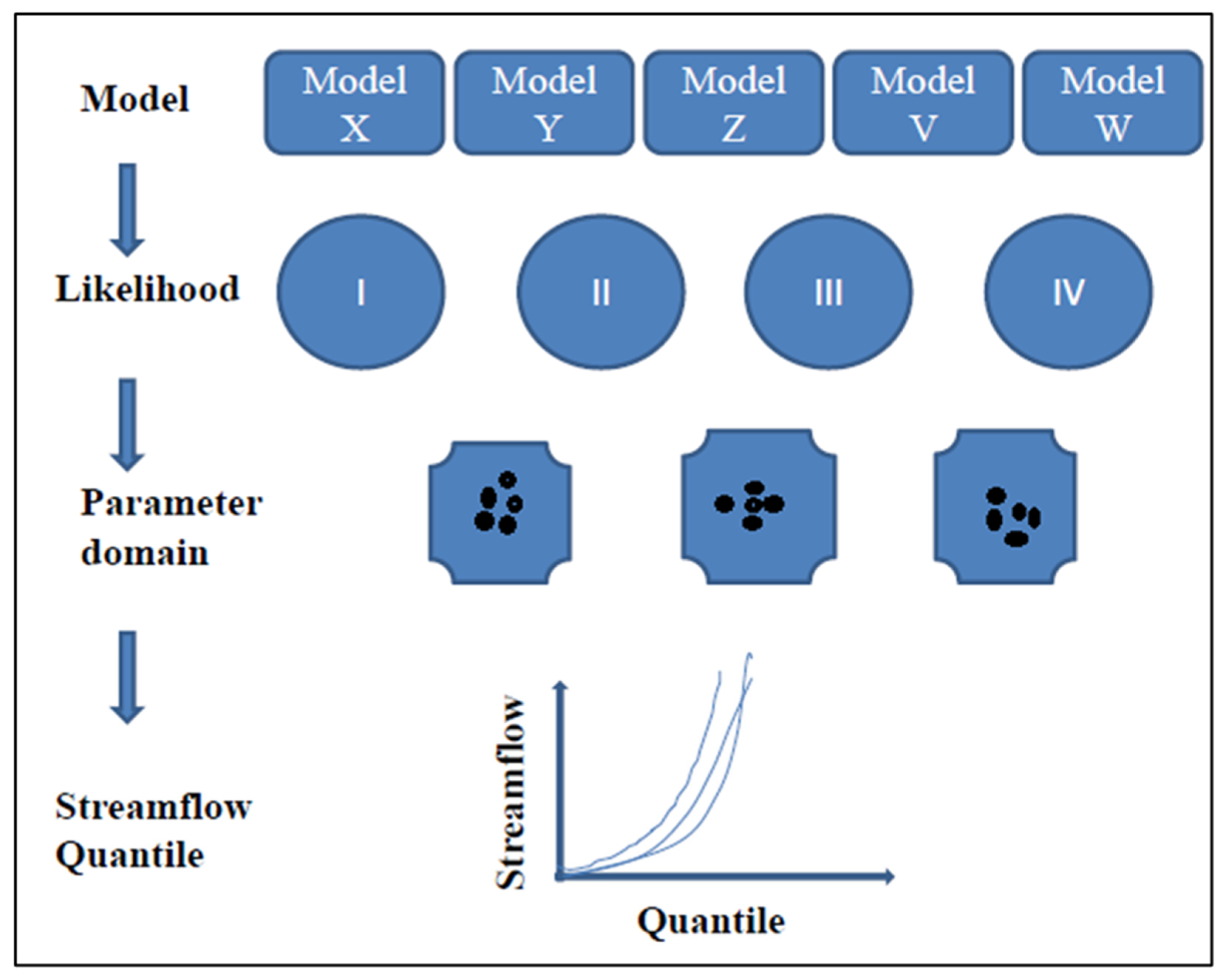
2.2. Conceptual Hydrological Model and Quantifying Input Uncertainty

Quantifying input uncertainty is vital in hydrologic models; therefore, several conceptual options were applied. Four parent hydrological models (TOPMODEL, ARNOXVIC, PRMS, SACRAMENTO) within the FUSE framework to represent the full spectrum of potential model [19] variability in the absence of specific information on the catchment hydrologic processes. Twenty-two (22) model parameters represent the hydrological system within FUSE [19]. Some of these parameters are inactive depending on the model configuration of interest. Figure 4 outlines the model structure that was considered in the simulation results presented. Flexibility in selecting model structure remains, as it is possible to use the framework for understanding structural errors [18,19,21,24]. The input of the models, such as precipitation (rainfall)/temperature/windspeed, was checked with the variability of different grids in a specified catchment or area compared to the true rainfall of the total catchment grids (Figure 4). At the same time, point gauge rainfall for that specific catchment was considered for the input variation [18,24]. Details of the four parent models could be found in [19].

The chosen experimental design is a combination of climate resilience, environmental sustainability, and water security modeling. The equation was based on the basics of the theoretical context of quantifying the metrics of the methodological framework. More details on [18,19,24].

For a given model (Figure 5), analyses were conducted for different likelihood or objective functions, including the Nash–Sutcliffe efficiency coefficient (NSE) [21], logarithmic Nash–Sutcliffe efficiency (LogNSE), and square root Nash–Sutcliffe efficiency (SqrtNSE). The optimization algorithm (dynamically dimension search (DDS)) was used to find the optimum parameter sets. From each simulation, the quantile variation of streamflow was determined and, thus, compared with different input variabilities of the defined catchment [18,24]. It is said that over-parameterization, dependency on input data bias, and lack of a systematic link between parameter precision and model efficiency are the three main factors [24,27] that complicate the regionalization of conceptual rainfall-runoff models. With the best possible model structure, input uncertainty was quantified to improve climate resilience.

As part of the demonstration of the approach, three objective functions were selected for analysis, including the Nash–Sutcliffe efficiency coefficient (NSE) [28], a logarithmic Nash–Sutcliffe efficiency (LogNSE), and a square root Nash–Sutcliffe efficiency (SqrtNSE). The Nash–Sutcliffe efficiency measures the relative magnitude of the model residual variance in comparison to the observed data variance. This efficiency can be greatly influenced by the peak flow values, which tend to have higher residual error. In contrast, the LogNSE and SqrtNSE are more likely to be influenced by low flows as the log and square root transformation reduces the importance of errors on larger flow magnitudes. These three objective functions are selected to reflect variability in the model optimization process and the desire to provide suitable models that fit different aspects of the hydrograph and the catchment response depending on the purpose of the model.

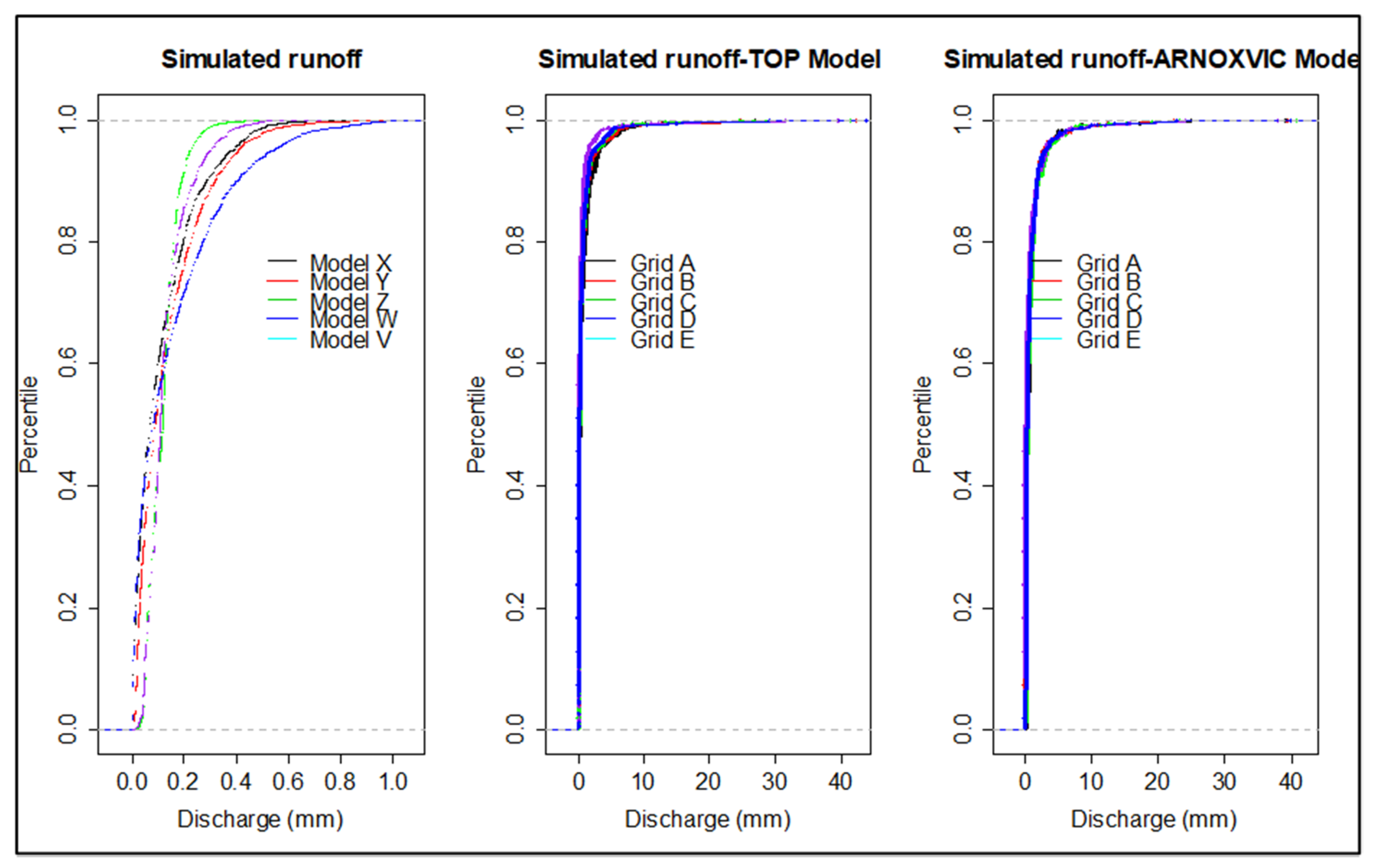
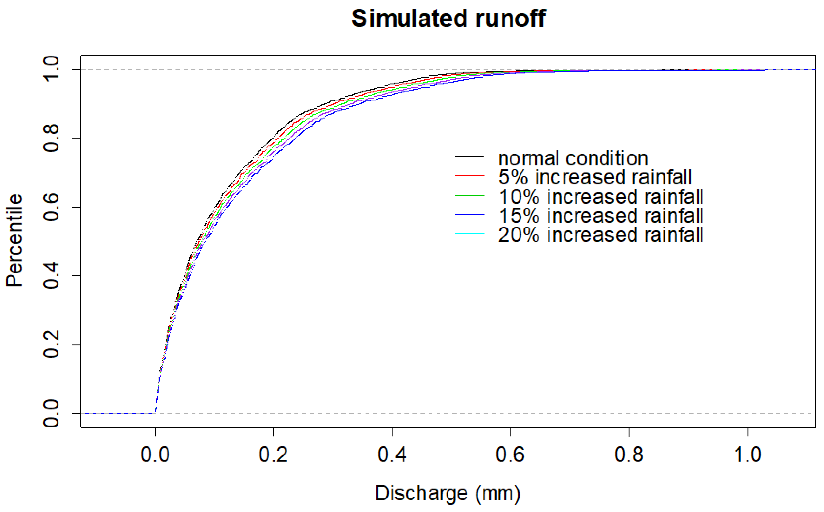
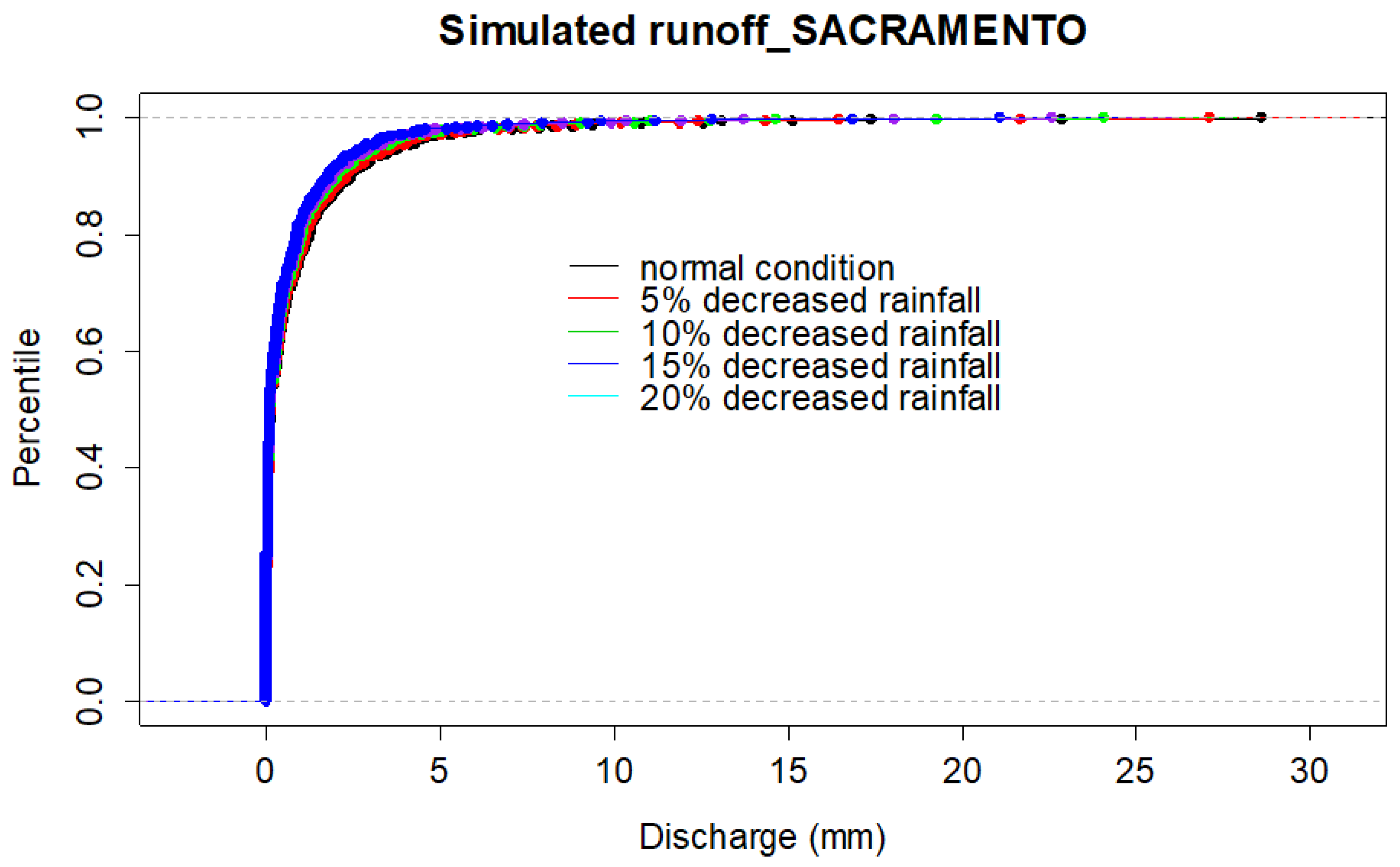
3. Results and Analysis

In this section, the key outcome is analyzed based on the method and data presented in the previous section. The more-generalized scenario was considered in this analysis. The possible scenarios were: (i) increasing precipitation, constant temperature; (ii) decreasing precipitation, constant temperature; (iii) increasing temperature, constant precipitation; (iv) decreasing temperature, constant precipitation; and (v) real-time variability with changing conditions.

Figure 6 contains three sub-plots. The left one shows the variability of streamflow/discharge among different developed models (X, Y, Z, W, and V) generated from four parent models. The right plot shows the regional variability of streamflow/discharge due to changing grid with respect to selected parent model ARNOXVIC and the middle one is similar to the right, only testing with different parent model name TOP model.

For a specific catchment (e.g., Richmond, NSW), different model structures responded differently to the variability (Figure 6, left) in predicting streamflow variability output. This represents higher prediction input uncertainty and the higher percentile and leads to more uncertainty in climate resiliency, with significant effects on environmental sustainability. By changing the different grid’s precipitation levels, variability was reduced (Figure 6, middle and right).

This Figure 7 shows the regional rainfall considering different scenarios to observe the variability of streamflow/discharge due to changing grid with respect to selected parent model PRMS.

Input variability in different model choices and grid-based rainfall variability with model input of rainfall was quantified with the variability of different grids in a specified catchment or area compared to true rainfall of total grids of the catchment. At the same time, point gauge rainfall was considered for the variation in input for each specific catchment (Figure 6, Figure 7 and Figure 8).

Catchment-to-catchment variability was observed due to variable catchment properties. For example, uncertainty in the Richmond catchment was high compared to the Seventeen Mile catchment due to climate variability; one catchment was very wet considering the metrics of quantile flow deviation (QFD) metric [18,19], and the other was very dry. Meanwhile, the Buchan River catchment in Melbourne, Victoria, was more similar to the Barambah River catchment of Queensland. Extreme input uncertainty was quantified by applying a dynamically dimensioned search optimization algorithm [18,19,24]. The analysis of the input uncertainty of four different catchments in Australia (Figure 2) showed the variability in uncertainty due to streamflow uncertainty [19,21,25]. The quantile flow deviation (QFD) metric [18,24,26] was used to estimate the input uncertainty compared to the model structure and parameter uncertainty [19]. This uncertainty was, directly and indirectly, linked with climate resilience and environmental sustainability and was quantified using Equations (1)–(3). Based on the extent of interaction, it is possible to integrate dynamic dimensions of water security modeling. Nash–Sutcliffe efficiency (NSE) has been presented for model simulations of discharge and is widely used to assess the predictive power of hydrological models. Additional analysis considering alternate objective functions to assess how sensitive our findings are to the objective function used is undertaken. NSE values vary in a range of 0.69 to 0.94 considering different catchments and selected model structures.

The three objective functions (NSE, LogNSE, SqrtNSE) are selected to reflect variability in the model optimization process and the desire to provide suitable models that fit different aspects of the hydrograph and the catchment response depending on the purpose of the model (Figure 9). As Figure 9 illustrates, the change in the proportion of uncertainty by considering additional objective functions is not significant.

However, an aggregate sustainability score could be computed based on multiple indicators organized into four dimensions: environment, social, water security and nutrition, and economic. In the multi-dimensional nature of the sustainability score, there was no “natural” or “theoretical” threshold above which a country could be said to be sustainable. In other words, the creation of the metric also highlights the urgent need for governments and other key stakeholders (donors, international development agencies, etc.) to invest in more comprehensive monitoring of the existing water-energy-food systems. Increased monitoring is particularly relevant concerning transformation, transport, retail, and distribution, for which data are still missing, including in some high-income-level countries. The optimal combination and technical validation are crucial for the final computation of the sustainability score [4,29,30].

4. Discussion—Scenarios of Model Development

As this study analyzed the model input and output uncertainty, this approach is useful for precision agriculture. How 1 mm of rainfall can influence cropping patterns and food production can be easily visualized for decision makers. Moreover, streamflow uncertainty has a direct linkage with climate resiliency. In this section, different aspects of the possible integration of the dynamic dimensions of water security were attributed to environmental sustainability and climate resilience. As water security is a multi-faceted dilemma, it goes further than the mere balancing of supply and demand [3,31,32]. On the contrary, static index-based approaches to quantifying water security are impotent to acknowledge the human action inherent to the water cycle. A more flexible and dynamic view of water security is urgent considering human adaptation to environmental change and increasing spatial specialization [3,31]. A four-dimensional dynamic space that maps sources, resource availability, infrastructure, and vibrant economic options is important in a climate-resilient sustainable agriculture domain. These dimensions are based on scenarios considering carbon emissions and possible trends in the world economy.

4.1. Water Security, Water Cycle Modifications, and Climate Resilience

Water security, climate resilience, and environmental sustainability must be closely interrelated for effective agricultural practice, identical to our body parts. As it is complex to quantify, we applied the function with its parameters then applied the regionalization approach to obtain the process extents (Figure 10). As global climate change intensifies, many countries have been hit hard by an unprecedented wave of droughts and water shortages. Water security can be defined as a function of different parameters as follows:

$$\mathrm{Water} \mathrm{Sec}\mathrm{urity}, \mathrm{W}=\mathrm{f} \left(\mathrm{R}, \mathrm{C}, \mathrm{E}, \mathrm{T}, \mathrm{G}, \mathrm{C}2, \mathrm{U}\right)$$

(6)

where R is resource, C is culture, E is economy, T is technology, G is governance, C2 is climate change, and U is uncertainty.

Establishing safe limits to water cycle modifications and identifying possible spatially explicit methods for quantification is an enormous challenge [33]. Many current and widely relied-upon hydrologic prediction approaches are founded on the assumption of stationarity [34], which permits extrapolation to the future using historical data. In a changing world, however, neither the structure (e.g., patterns of land use and land cover, connectivity between channels, and riparian or wetland environments, or the extent of human-made structures) nor the external drivers (e.g., temperature and precipitation forcing) of the hydrologic response can be treated as fixed [18,19,20,21,22,24,25,26,35]. Instead, changes in structure and drivers create the potential for new dynamics [36], for example, by hydrologic systems crossing unknown thresholds [19,26,31]. The possibility for the emergence of such new dynamics poses key challenges to predictability, especially on decadal or longer time scales.

Understanding the bloodstream interdependency, availability, and accessibility of surface water and groundwater plays a crucial role in recognizing and managing water security. The Falkenmark water stress index, defined as the per capita annual renewable freshwater available, was an early effort to recognize the relationship between human needs and environmental constraints; regions with less than 1000 m³ per capita per year were defined as “water-scarce” [35,37]. As populations grow, humanity faces the prospect of uncertain future water supplies due to climate change and the increasing demands on water [35,38,39]. In the virtual water importing and exporting region, some factors dominate the water balance, affecting water security. For example, Murray Darling Basin is considered the food bowl for Australia, where ecological destruction, environmental regulations, laws, community sensitivity, infrastructure, controls on abstraction, and climate change impacts play a key role in the water security domain (Figure 10). This phenomenon instigates the internal integration of the dynamic dimensions of water security modeling with the variability of climate resilience and environmental sustainability.

4.2. Climate–Water Quality Relationships in Changing Streamflow

Temperature and precipitation elasticities of water quality parameters, highlighted by N and P nutrients, can be analyzed in large rivers due to the change of streamflow. The spatial and temporal assessments show that precipitation elasticity is more variable in space than temperature elasticity and that seasonal variation is more evident for precipitation elasticity than temperature elasticity [1,32,34,36]. Even small changes to streamflow may have significant agricultural and ecological implications [38]. Therefore, it is vital to integrate the dynamic dimension of water security modeling with climate resiliency and environmental sustainability. It is potentially helpful for investigating the effects of climate change on water quality in large rivers, such as the long-term shift in nutrient concentrations.

4.3. Drought Management

Underestimation of solar radiation usually overestimates soil moisture. The concept of reliability-resilience-vulnerability (RRV) is used here in the context of agricultural drought through the analysis of temporal variations in soil moisture. The failure, or unsatisfactory stage, is considered the depletion of soil moisture below the permanent wilting point (PWP), an indicator of agricultural drought (Figure 10). The natural integration of water security modeling with climate resilience and ensuring environmental sustainability integrates the plant, soil, and atmospheric conditions at a particular location with the long-term, spatiotemporal variation of drought susceptibility [3,8,9,26].

5. Conclusions

The development of a decision support system (DSS) using advanced computer data processing tools and Internet systems to analyze large data sets has made the agriculture industry more sustainable. Increased land-use change with industrial development has made sustainable development critical. High-level policy intervention is required, considering climate change. Based on development trends, variability in climate extremes, and water security, a coordinated policy matrix is crucial. Integrating the available resources with the required products could be more effective with the application of a central database using DSS. Considering the diversity in an uncertain world, integrating dynamic dimensions of water security modeling is vital for ensuring environmental sustainability and the associated full range of climate resilience. This is also possible with the use of high-tech computer and Internet systems. This study presents a framework for integrating the dynamic dimensions of water security modeling with climate resilience and environmental sustainability variability. Therefore, a vital contribution of this paper is in accounting for the water security modeling and scenarios of model development. A more flexible and dynamic view of water security is urgent considering human adaptation to environmental change and increasing spatial specialization. With the adoption of high-tech computer data processing, including Internet systems, nature-based solutions can be more effective to model the dynamic indicators as outcomes of coupled human-water systems. Ensuring water security ease, the way of environmental sustainability paradigm. Quantifying the uncertainty in water availability or use projection gives the overall picture of the available water. Thereby, decision makers got the idea of available water for the effective and efficient use of water through enforcing water metering by adopting an integrated water pricing policy. As the amount of water demand is increasing in all sectors, including agriculture, new technology could be used for maximizing water use. This framework will surely help in the policymaking process to allocate the right share of water as per demand to save water, ensuring integrated water management. We have the options of multi-model structures considering four parent models, which gives the policymaker to adopt new model structures according to the purpose of the users. One of this study’s shortcomings was finding the real-time data of social structure and economic diversity to interlink the hydrological phenomena of climate and land-use change. Future research will concentrate on the nonlinear dimensions of food security, integrating climate resilience and water security in a sustainable domain.

References

1. Wang, L.; Zhang, M.; Li, Y.; Xia, J.; Ma, R. Wearable multi-sensor enabled decision support system for environmental comfort evaluation of mutton sheep farming. Comput. Electron. Agric. 2021, 187, 106302. [Google Scholar] [CrossRef]
2. Jin, G.; Chen, K.; Wang, P.; Guo, B.; Dong, Y.; Yang, J. Trade-offs in land-use competition and sustainable land development in the North China Plain. Technol. Forecast. Soc. Chang. 2019, 141, 36–46. [Google Scholar] [CrossRef]
3. Srinivasan, V.; Konar, M.; Sivapalan, M. A dynamic framework for water security. Water Secur. 2017, 1, 12–20. [Google Scholar] [CrossRef]
4. Zhou, L.; Tokos, H.; Krajnc, D.; Yang, Y. Sustainability Performance Evaluation in Industry by Composite Sustainability Index. Clean Technol. Environ. Pol. 2012, 14, 789–803. [Google Scholar] [CrossRef]
5. Resilience for Sustainability. Nat. Plants 2021, 7, 101. [CrossRef]
6. Intergovernmental Panel on Climate Change (IPCC). Summary for Policymakers. In Global Warming of 1.5 °C; Masson-Delmotte, V., Ed.; World Meteorological Organization: Geneva, Switzerland, 2018. [Google Scholar]
7. Chaudhary, A.; Gustafson, D.; Mathys, A. Multi-indicator sustainability assessment of global food systems. Nat. Commun. 2018, 9, 848. [Google Scholar] [CrossRef] [PubMed] [Green Version]
8. Gleeson, T.; Wang-Erlandsson, L.; Porkka, M.; Zipper, S.C.; Jaramillo, F.; Gerten, D. Illuminating water cycle modifications and Earth system resilience in the Anthropocene. Water Resour. Res. 2020, 56, e2019WR024957. [Google Scholar] [CrossRef] [Green Version]
9. Dabson, B.; Heflin, M.C.; Miller, K.K. Regional Resilience: Research and Policy Brief. 2012. Available online: http://nado.org/wp-content/uploads/2012/04/RUPRI-Regional-Resilience-Research-Policy-Brief.pdf (accessed on 15 February 2022).
10. Church, J.A. Sea Level Change. In Climate Change 2013: The Physical Science Basis; Stocker, T.F., Ed.; Cambridge University Press: Cambridge, UK, 2013; p. 1535. Available online: http://www.climatechange2013.org/images/report/WG1AR5_ALL_FINAL.pdf (accessed on 15 February 2022).
11. Finka, M.; Tóth, A. Regional Resiliences Improvement by Innovative Approaches in Management of External Shocks. 2014. Available online: http://www.spa-ce.net/pdf/2014/Conference_%202014/Toth_Spa-ce.net-2014.pdf (accessed on 15 February 2022).
12. Martin, R. Regional economic resilience, hysteresis and recessionary shocks. J. Econ. Geogr. 2012, 12, 1–32. [Google Scholar] [CrossRef]
13. Patterson, J.L.; Kelleher, P.A. Deeper Meaning of Resilience. In Resilient School Leaders: Strategies for Turning Adversity into Achievement; E-Book; Association for Supervision and Curriculum Development: Alexandria, VA, USA, 2005; Available online: http://www.ascd.org/publications/books/104003/chapters/A-Deeper-Meaning-of-Resilience.aspx (accessed on 15 February 2022).
14. Intergovernmental Panel on Climate Change (IPCC). Climate Change 2007: The Physical Science Basis; Contribution of Working Group I to the Fourth Assessment Report of the Intergovernmental Panel on Climate Change; Cambridge University Press: New York, NY, USA, 2007. [Google Scholar]
15. Field, C.B.; Barros, V.; Stocker, T.F.; Dahe, Q. Managing the Risks of Extreme Events and Disasters to Advance Climate Change Adaptation; Cambridge University Press: Cambridge, UK, 2012; p. 582. [Google Scholar]
16. Wong, P.P.; Losada, I.J.; Gattuso, J.-P.; Hinkel, J.; Khattabi, A.; McInnes, K.L.; Saito, Y.; Sallenger, A. Coastal Systems and Low-Lying Areas. In Climate Change 2014: Impacts, Adaptation, and Vulnerability; Field, C.B., Barros, V.R., Dokken, D.J., Mach, K.J., Mastrandrea, M.D., Bilir, T.E., Chatterjee, M., Ebi, K.L., Estrada, Y.O., Genova, R.C., et al., Eds.; Cambridge University Press: Cambridge, UK; New York, NY, USA, 2014; pp. 361–409. Available online: https://www.ipcc.ch/site/assets/uploads/2018/02/WGIIAR5-Chap5_FINAL.pdf (accessed on 15 February 2022).
17. Kundzewicz, Z.W.; Mata, L.J.; Arnell, N.W.; DÖLl, P.; Jimenez, B.; Miller, K.; Oki, T.; ŞEn, Z.; Shiklomanov, I. The implications of projected climate change for freshwater resources and their management. Hydrol. Sci. J. 2008, 53, 3–10. [Google Scholar] [CrossRef]
18. Shoaib, S.A.; Marshall, L.; Sharma, A. A metric for attributing variability in modelled streamflows. J. Hydrol. 2016, 541, 1475–1487. [Google Scholar] [CrossRef]
19. Clark, M.P.; Slater, A.G.; Rupp, D.E.; Woods, R.A.; Vrugt, J.A.; Gupta, H.V.; Wagener, T.; Hay, L.E. Framework for Understanding Structural Errors (FUSE): A modular framework to diagnose differences between hydrological models. Water Resour. Res. 2008, 44, W00B02. [Google Scholar] [CrossRef]
20. Sivakumar, B. Global climate change and its impacts on water resources planning and management: Assessment and challenges. Stoch Env. Res. Risk Assess. 2011, 25, 583–600. [Google Scholar] [CrossRef]
21. Clark, M.P.; McMillan, H.K.; Collins, D.B.G.; Kavetski, D.; Woods, R.A. Hydrological field data from a modeller’s perspective: Part 2: Process-based evaluation of model hypotheses. Hydrol. Processes 2011, 25, 523–543. [Google Scholar] [CrossRef]
22. Woldemeskel, F.M.; Sharma, A.; Sivakumar, B.; Mehrotra, R. An error estimation method for precipitation and temperature projections for future climates. J. Geophys. Res. Atmos. 2012, 117, D22104. [Google Scholar] [CrossRef]
23. The 2015 FM Resilience Index. Annual Report, Oxford Metrica. 2015. Available online: https://www.fmglobal.com/assets/pdf/Resilience_Methodology.pdf (accessed on 15 February 2022).
24. Shoaib, S.A.; Marshall, L.; Sharma, A. Attributing input uncertainty in streamflow simulations via the Quantile Flow Deviation metric. Adv. Water Res. 2018, 116, 40–55. [Google Scholar]
25. Clark, M.P.; Kavetski, D.; Fenicia, F. Pursuing the method of multiple working hypotheses for hydrological modeling. Water Resour. Res. 2011, 47, W09301. [Google Scholar] [CrossRef] [Green Version]
26. Shoaib, S.A.; Khan, M.Z.K.; Sultana, N.; Mahmood, T.H. Quantifying Uncertainty in Food Security Modeling. Agriculture 2021, 11, 33. [Google Scholar] [CrossRef]
27. Andréassian, V.; Perrin, C.; Oudin, L. From catchment similarity to hydrological similarity: A review of the difficulties hindering the regionalization of hydrological models. Geophys. Res. Abstr. 2003, 13. Available online: https://meetingorganizer.copernicus.org/EGU2011/EGU2011-13991.pdf (accessed on 15 February 2022).
28. Nash, J.E.; Sutcliffe, J.V. River flow forecasting through conceptual models part I—A discussion of principles. J. Hydrol. 1970, 10, 282–290. [Google Scholar] [CrossRef]
29. Xiaoyu, G. When to Use What: Methods for Weighting and Aggregating Sustainability Indicators. Ecol. Indic. 2017, 81, 491–502. [Google Scholar]
30. Sirone, S.; Seppala, J.; Leskinen, P. Towards More Non-Compensatory Sustainable Society Index. Environ. Dev. Sustain. 2015, 17, 587–621. [Google Scholar] [CrossRef]
31. Wagener, T.; Sivapalan, M.; Troch, P.A.; McGlynn, B.L.; Harman, C.J.; Gupta, H.V.; Kumar, P.; Rao, P.S.C.; Basu, N.B.; Wilson, J.S. The future of hydrology: An evolving science for a changing world. Water Resour. Res. 2010, 46, W05301. [Google Scholar] [CrossRef]
32. Morrison, R.R.; Stone, M.C. Spatially implemented Bayesian network model to assess environmental impacts of water management. Water Resour. Res. 2014, 50, 8107–8124. [Google Scholar] [CrossRef]
33. Savenije, H.H.; Hoekstra, A.Y.; van der Zaag, P. Evolving water science in the Anthropocene. Hydrol. Earth Syst. Sci. 2014, 18, 319–332. [Google Scholar] [CrossRef] [Green Version]
34. Sivapalan, M.; Savenije, H.H.; Blöschl, G. Socio-hydrology: A new science of people and water. Hydrol. Processes 2012, 26, 1270–1276. [Google Scholar] [CrossRef]
35. Falkenmark, M.; Lundqvist, J.; Widstrand, C. Macro-scale water scarcity requires micro-scale approaches: Aspects of vulnerability in semi-arid development. Nat. Resour. Forum 1989, 13, 258–267. [Google Scholar] [CrossRef]
36. Sivapalan, M.; Konar, M.; Srinivasan, V.; Chhatre, A.; Wutich, A.; Scott, C.A.; Wescoat, J.L.; Rodríguez-Iturbe, I. Socio-hydrology: Use-inspired water sustainability science for the Anthropocene. Earths Future 2014, 2, 225–230. [Google Scholar] [CrossRef] [Green Version]
37. Falkenmark, M.; Rockström, J. The new blue and green water paradigm: Breaking new ground for water resources planning and management. J. Water Resour. Plan. Manag. 2006, 132, 129–132. [Google Scholar] [CrossRef]
38. Manzoni, S.; Katul, G.; Porporato, A. A dynamical system perspective on plant hydraulic failure. Water Resour. Res. 2014, 50, 5170–5183. [Google Scholar] [CrossRef]
39. Michel-Kerjan, E. How resilient is your country? Nature 2012, 491, 497. Available online: http://0-www-nature-com.brum.beds.ac.uk/news/how-resilient-is-your-country-1.11861 (accessed on 15 February 2022). [CrossRef] [Green Version]
Figure 1. Integration of climate resilience with water security and environmental sustainability.
Agriculture 12 00303 g001
Figure 2. Study area of selected Australian catchment. Four catchments were considered in the study: (i) Richmond, New South Wales, (ii) Buchan River Victoria, (iii) Seventeen Mile Creek, a waterfall view, Northern Territory, (iv) Barambah Creek at Litzows, Queensland.
Agriculture 12 00303 g002
Figure 3. Schematic overview of the experimental design undertaken to find a sustainable solution and quantify the resilience index for input variability. Climate extreme ensembles are analyzed as a function of resilience functions and optimized with different solutions. All the solutions are characterized as the resilience index with time. The circle in the bottom panel of the figure shows the increase in complexity from left to right. Ensembles of solutions are possible with multiple climate extreme possibilities for a specific catchment or community.
Agriculture 12 00303 g003
Figure 4. Multi-model structure built to model catchment processes. Details of the different component multi-model structures are (i) single state (SS), (ii) separate tension storage (ST), (iii) cascading buckets (CB), (iv) baseflow reservoir of fixed size (BRFS), (vi) tension reservoir plus two parallel tanks (TRTPT), (vii) baseflow reservoir of unlimited size (frac rate) (BRUSfr), (viii) baseflow reservoir of unlimited size (power recession) (BRUSpr), (ix) drainage above field capacity (DAFC), (x) gravity drainage (GD), (xi) saturated zone control (SZC), (xii) unsaturated zone Pareto (UZP), (xiii) unsaturated zone linear (UZL), (xiii) saturated zone topographic (SZT). Model structural components used for the 4 models considered in this study are depicted as TOPMODEL = a; ARNOXVIC = b; PRMS = c; SACRAMENTO = d (after [18]).
Agriculture 12 00303 g004
Figure 5. Possible model structure options in hydrological models with alternate descriptions for upper and lower soil layers, types of surface runoff, vertical drainage, evaporation, interflows, and possible routing options. For different conceptual model structures, different likelihood/objective functions can be made. For each likelihood, options of parameter domain can be generated. For each simulation, flow quantiles can be produced to compare with different inputs.
Agriculture 12 00303 g005
Figure 6. Input variability in different model choices and grid-based rainfall variability with the model input of rainfall estimated with the variability of different grids in a specified catchment or area compared to true rainfall of the total grids of the catchment. At the same time, point gauge rainfall for that specific catchment is considered for the variation in input.
Agriculture 12 00303 g006
Figure 7. Input rainfall variability to see the changeability of discharge in a defined model.
Agriculture 12 00303 g007
Figure 8. Input rainfall variability (decreasing trend) to observe the changeability of discharge in a defined SACRAMENTO model. Changing rainfall variability is also observed to obtain the overall picture.
Agriculture 12 00303 g008
Figure 9. Impact of objective function variability considering model structure, identifiability/parameter, and their interactions.
Agriculture 12 00303 g009
Figure 10. Interaction among drivers of water security that lead to food security for Australia: resource, economy, culture, technology (advancement of computer and Internet use), and governance. After [3].
Agriculture 12 00303 g010
Publisher’s Note: MDPI stays neutral with regard to jurisdictional claims in published maps and institutional affiliations.