Article

Tea Bud Detection and 3D Pose Estimation in the Field with a Depth Camera Based on Improved YOLOv5 and the Optimal Pose-Vertices Search Method

1
School of Mechanical Engineering, Zhejiang Sci-Tech University, Hangzhou 310018, China
2
Tea Research Institute, Chinese Academy of Agricultural Sciences, Hangzhou 310008, China
*
Author to whom correspondence should be addressed.
Submission received: 6 June 2023 / Revised: 12 July 2023 / Accepted: 13 July 2023 / Published: 14 July 2023
(This article belongs to the Special Issue Advances in Agricultural Engineering Technologies and Application)

Abstract

:
The precise detection and positioning of tea buds are among the major issues in tea picking automation. In this study, a novel algorithm for detecting tea buds and estimating their poses in a field environment was proposed by using a depth camera. This algorithm introduces some improvements to the YOLOv5l architecture. A Coordinate Attention Mechanism (CAM) was inserted into the neck part to accurately position the elements of interest, a BiFPN was used to enhance the small object detection ability, and a GhostConv module replaced the original Conv module in the backbone to reduce the model size and speed up model inference. After testing, the proposed detection model achieved an mAP of 85.2%, a speed of 87.71 FPS, a parameter number of 29.25 M, and a FLOPs value of 59.8 G, which are all better than those achieved with the original model. Next, an optimal pose-vertices search method (OPVSM) was developed to estimate the pose of tea by constructing a graph model to fit the pointcloud. This method could accurately estimate the poses of tea buds, with an overall accuracy of 90%, and it was more flexible and adaptive to the variations in tea buds in terms of size, color, and shape features. Additionally, the experiments demonstrated that the OPVSM could correctly establish the pose of tea buds through pointcloud downsampling by using voxel filtering with a 2 mm × 2 mm × 1 mm grid, and this process could effectively reduce the size of the pointcloud to smaller than 800 to ensure that the algorithm could be run within 0.2 s. The results demonstrate the effectiveness of the proposed algorithm for tea bud detection and pose estimation in a field setting. Furthermore, the proposed algorithm has the potential to be used in tea picking robots and also can be extended to other crops and objects, making it a valuable tool for precision agriculture and robotic applications.

1. Introduction

Tea is a popular beverage consumed worldwide and also a vital economic crop for many countries. In comparison to the high demand and output of tea, the traditional method of harvesting tea leaves remains quite rudimentary, particularly for famous teas, which are often picked manually. This picking process is labor-intensive, time-consuming, and physically demanding, which may result in strains and injuries among laborers. Instead of picking manually, an automatic tea picking system has the potential to lower the requirement of labor and ease labor intensity [1]. In order to develop this automatic system, detecting and positioning the tea leaves in 3D space is an essential process, which allows the system to accurately perceive the leaves in the field for picking. Moreover, the algorithm for detecting and positioning tea leaves can be used to enhance production, facilitate research, and monitor and preserve the environment. Research into tea detection and positioning algorithms plays a crucial role in automatic picking systems, which have the potential to significantly improve the efficiency and productivity of tea production in the future [2].
The development of tea bud detectors has been sustained for several years. Researchers have extracted and combined various features, such as shape, color, and texture, from tea bud images to design advanced features using complicated processes. For example, Zhang et al. utilized R-B factors to convert the image to grayscale and performed threshold segmentation using the Otsu method. They applied area filtering, erosion, and expansion algorithms to generate a binary image of the tea buds. Finally, the center of mass method was employed to determine the position of the tea buds within the binary image [3]. Zhang et al. applied a Gaussian filter to reduce image noise and split the images into their respective R, G, and B components. Image operations were performed to obtain G-B’ components. The minimum error method was utilized to determine the most suitable adaptation thresholds, which underwent a piecewise linear transformation to enhance the distinction between the tea buds and the background. Binarization and the application of the Canny operator were then employed to detect edges in the binary image. Finally, the unknown area was calculated and marked, and the segmentation process was completed using the watershed function [4]. Wu et al. analyzed the color information of G and G-B components of tea buds and leaves. They calculated segmentation thresholds using an improved Otsu method to recognize tea buds [5]. While these methods have demonstrated effectiveness under specific conditions, their limited generalizability and lack of intelligence restrict their applicability in production scenarios.
With the progression of deep learning methods, the object detection field has shifted the focus toward acquiring larger labeled datasets and refining the network architecture, rather than emphasizing image features. Many studies on object detection have used large public datasets to train and test detectors based on convolutional networks, with subjects such as cars [6], traffic signs [7] and pedestrians [8]. Similarly, many studies on object detection based on deep learning in agriculture have also been conducted [9]. Zeng et al. proposed using a lightweight YOLOv5 model to efficiently detect the location and ripeness of tomato fruits in real time, and the improvement reduced the model size by 51.1% while maintaining a 93% true detection rate [10]. Ma et al. integrated a coordinate attention (CA) module with YOLOv5 and trained and tested a YOLOv5-lotus model to effectively detect overripe lotus seedpods in a natural environment [11]. Wang et al. introduced an apple fruitlet detection method that utilizes a channel-pruned YOLOv5s deep learning algorithm, achieving rapid and accurate detection, and the compact model size of 1.4 MB facilitated the development of portable mobile fruit thinning terminals [12]. Sozzi et al. evaluated six versions of YOLO (YOLOv3, YOLOv3-tiny, YOLOv4, YOLOv4-tiny, YOLOv5x, and YOLOv5s) for real-time bunch detection and counting in grapes. Finally, YOLOv4-tiny emerged as the best choice due to its optimal balance between accuracy and speed. This study provided valuable insights into the performance of different YOLO versions and their applicability in the grape industry [13]. Cardellicchio et al. used single-stage detectors based on YOLOv5 to effectively identify nodes, fruit, and flowers on a challenging dataset acquired during a stress experiment conducted on multiple tomato genotypes, and achieved relatively high scores [14].
In particular, studies on the detection of tea buds based on deep learning have also made some significant advancements. Murthi and Thangavel employed the active contour model to identify potential tea bud targets in images, then utilized a DCNN for recognition [15]. Chen et al. introduced a new fresh tea sprout detection method, FTSD-IEFSSD, which integrates image enhancement and a fusion single-shot detector. This method separately inputs the original and enhanced images into a ResNet50 subnetwork and improves detection accuracy through score fusion. This method achieved an AP of 92.8% [16]. Xu et al. combined YOLOv3 with DenseNet201 to quickly and accurately detect and classify tea buds, achieving 82.58% precision on the top-shot dataset and 99.28% precision on the side-shot dataset [17]. Gui et al. enhanced and reduced the weight of the YOLOv5 network for tea bud detection by replacing the standard convolution with a Ghost_conv module, adding a BAM into the backbone, applying MS-WFF in the neck, and switching to a CIOU loss function. After training and testing on a dataset of 1000 samples, the model achieved a frame rate of 29,509 FPS, an mAP of 92.66%, and a model size of 90 M [18]. Moreover, tea buds can also be segmented using deep learning. Hu et al. presented a discriminative pyramid (DP) network-based method with exceptional accuracy for the semantic segmentation of tea geometrids in natural scene images [19], while TS-SegNet, a novel deep convolutional encoder-decoder network method for tea sprout segmentation proposed by Qian et al., produced a good segmentation result [20].
Currently, research is primarily focused on detecting and segmenting tea buds, with very few studies proposing methods for identifying the specific points for picking. However, identifying the position of the picking point is crucial for efficient and effective tea bud harvesting. The Faster R-CNN was used to locate tea shoot picking points in the field, achieving a precision of 79% [21], and the Mask-RCNN was utilized to create a recognition model for tea buds, leaves, and picking points. The results showed an average detection accuracy of 93.95% and a recall rate of 92.48% [22]. Although these algorithms position the picking point of tea buds in the image, the lack of a depth sensor limits the acquisition of spatial coordinates for picking points. Thus, the robot would be unable to determine the target position in robot coordinates for end-effector movement. Li et al. used the YOLO network to detect the tea buds and acquired the position of the target in the 3D space by using an RGB-D camera [23]. This method calculates the center point of all points and represents the grab position using a vertical minimum circumscribed cylinder. Then, they inclined the minimum circumscribed cylinder according to the growth direction of tea buds calculated via the PCA method [24]. Chen et al. developed a robotics system for the intelligent picking of tea buds, training the YOLOv3 model to detect the tea buds from images and proposing an image algorithm to locate the picking point. While their system has a successful picking rate of 80%, the detection precision of this system could be improved, and the importance of addressing measurement errors and motion errors in the picking process should not be overlooked [25].
In conclusion, tea bud detection research has experienced good development, but some datasets are still quite simple and small-sized. Moreover, the pose of tea buds within a 3D space is important for the robot to grasp the target accurately, yet there are few studies that have talked about this issue. Therefore, the aim of this study is to detect tea buds using an improved YOLOv5 network and determine their 3D pose through the OPVSM. The contributions of this study are as follows:
  • The convolution (CBS) of YOLOv5 is replaced by GhostConv to reduce FLOPs and compress the model size by generating more feature maps from cheap operations [26].
  • The Coordinate Attention Mechanism (CAM) is integrated into the neck, which could accurately locate the region of interest by reserving the coordinates of elements in the feature map, leading to more precise detection results [27].
  • The conversion from PANet to BiFPN enhances feature aggregation and multi-scale feature fusion, resulting in improved detection efficiency [28].
  • The OPVSM is proposed to search the pose-vertices from the pointcloud to build the skeleton of tea buds.

2. Materials and Methods

2.1. Improvement of YOLOv5

2.1.1. YOLOv5

As the most popular network architecture for object detection, the YOLOv5 (You Only Look Once) network model [29] is widely used in detection and recognition systems in various fields, as shown in Figure 1. This model architecture has spawned many improved versions because of its good modifiability, portability and trainability. This model provides two hyperparameters, the depth-multiple and width-multiple, used to control the depth (number of bottlenecks) and width (number of channels) of the backbone in the model, respectively.
Figure 1 shows the structure of the original YOLOv5 model. This model can be divided into four parts, including the input, backbone, neck and head. During training, the input part reads the images and labels, enhances these images and puts them into the backbone part. The backbone network extracts the features from images by means of the CSPDarknet53, which is composed of CSP modules. In the neck, FPN and PANet are used to aggregate image features and output three layers of feature maps with different sizes. Finally, the head part predicts and outputs the detection results according to these feature maps.

2.1.2. Architecture of Improved YOLOv5

Although the YOLOv5 model has good precision and speed, its performance in small target detection is inadequate. Figure 2 shows the structure of the improved YOLOv5 model. The main modifications are made in the backbone and neck parts of the model. In Figure 2, the red circle 1 represents the Coordinate Attention Mechanism (CAM). It is incorporated into the neck section to precisely locate the region of interest by preserving the coordinates of elements in the feature map, thereby improving the accuracy of object detection. Meanwhile, the red circle 2 denotes the modified connection known as BiFPN. It replaces the PANet in the neck to enhance feature aggregation and multi-scale feature fusion. Additionally, the red circle 3 represents the GhostConv module utilized in the backbone. It replaces the standard convolution (CBS) in the backbone, which reduces the computation cost by generating more feature maps from cheap operations. These modifications improve the small target detection performance of the YOLOv5 model and make it more efficient.

2.1.3. Coordinate Attention Mechanism

At the beginning of the neck section, the Coordinate Attention Mechanism (CAM) shown in Figure 3 is added. Firstly, the variables with a size of H × W × C are shrunk in the X and Y directions using separate adaptive average pooling layers. Here, the X direction corresponds to the width of the feature map, while the Y direction corresponds to its height. Two feature maps with different sizes of H × 1 × C and 1 × W × C are then obtained.
Next, the Y-pooling feature map is permuted and aggregated with the X-pooling feature map to create a new feature map with a size of (H + W) × 1 × C. This aggregated feature is then processed using a CBS consisting of a convolution layer, batch normalization layers, and the SiLU activation function. The SiLU function applies the sigmoid function to the input value x and multiplies the result with the input itself, providing smoothness and non-linearity, and preserving certain linearity characteristics suitable for deep learning models.
Following this, the feature map is split back into two feature maps of the same size as before the aggregation step. The previously permuted feature map is restored to its original size. Finally, the two feature maps are combined element-wise with the original feature map to generate a new feature map with a size of H × W × C, incorporating aggregated contextual information.
The Coordinate Attention Mechanism utilizes a separate global pooling operation in the X and Y directions, respectively, so that the attention module can retain the element position of the precise coordinates in the feature map. The formula for the separate global pooling operation is as follows:
z c h h = 1 W 0 i < W x c h , i z c w w = 1 H 0 j < H x c j , w
More precisely, the above pooling operation is an information embedding process in the attention module. The subsequent matrix transformations such as Concat and CBS are used to aggregate the contextual information. After these operations, the region of interest can be obtained on the basis of the features generated by the pooling. In brief, this structure is more conducive to accurately positioning the elements of interest.
The Coordinate Attention Mechanism (CAM) captures and leverages spatial information by utilizing separate global pooling operations in the X and Y directions. This allows the CAM to emphasize or suppress specific spatial locations based on their importance. Unlike other attention mechanisms such as Efficient Channel Attention (ECA), Squeeze-and-Excitation (SE), or Convolutional Block Attention Module (CBAM), which primarily focus on channel-wise attention, the CAM specifically targets spatial reasoning. By incorporating CAM, this model gains the ability to perform precise localization and spatial reasoning, which are particularly valuable in tasks requiring accurate object detection and a good understanding of spatial relationships. Additionally, CAM exhibits high effectiveness in localizing important features within an input feature map. By applying separate global pooling in the X and Y directions, the CAM attends to specific spatial locations, enabling the model to capture fine-grained details and accurately localize objects. In contrast, other attention mechanisms like ECA, SE, or CBAM may not explicitly prioritize precise localization, limiting their performance in tasks where precise object localization is crucial. Furthermore, the separate global pooling operations in the X and Y directions enable efficient computation, as they do not require extensive calculations across channels or intricate transformations. This leads to improved efficiency, reduced memory consumption, and faster inference times, making CAM particularly suitable for real-time applications. Overall, compared to other attention mechanisms, CAM demonstrates stronger spatial reasoning ability, higher localization accuracy, and lower computational complexity. It is particularly suitable for tea bud detection.

2.1.4. BiFPN

The bidirectional feature pyramid network (BiFPN) improves the FPN by incorporating a bidirectional feature fusion approach. It deletes the feature maps with single inputs, adds the extra connection between original and final feature maps, and down-samples the original feature map to make the network more accurate and efficient. In this study, the BiFPN is adapted and ported based on the PANet in the neck part to improve the detection efficiency and the muti-scale feature fusion. As shown in Figure 4, the relationship drawn by the red dotted arrow is the new improved connection. This new connection is utilized to aggregate more features in the middle scale layer for enhancing the small object detection ability without increasing the computational cost too much.
Specifically, unlike the unidirectional flow of information in the original FPN, BiFPN enables bidirectional information flow, allowing it to propagate in both bottom-up and top-down directions. Moreover, it efficiently combines features from different levels of the pyramid, incorporating both top-down and bottom-up pathways as well as lateral connections. This multi-scale fusion process enables effective feature capture at various scales, facilitating the network’s ability to handle objects of different sizes. Additionally, BiFPN is designed to be computationally efficient by reducing overheads through shared computations across multiple feature levels, distinguishing it from other fusion approaches. Furthermore, BiFPN addresses FPN’s limitations by introducing extra connections between adjacent levels of the pyramid, facilitating improved information propagation across scales for the transmission of fine-grained details between higher-level and lower-level feature maps. Therefore, in this study, BiFPN enhances the expressive power, adaptability, and efficiency of the feature fusion process, improving the model’s ability to detect small objects. This improvement is particularly valuable for tea bud detection, reducing the rate of missed detections.

2.1.5. GhostConv

GhostConv can be viewed as a factorization of the CBS block into two parts, where one part has a large number of filters but fewer channels, and the other part has fewer filters but more channels. This factorization allows for a reduction in the number of parameters and computational cost, while maintaining a good balance between representation power and efficiency. As shown in Figure 5, the CBS block convolves the feature maps from C channels to C/2 channels by reducing the number of kernels. Then, the DWConv (depth-wise convolution) block is applied to each channel of the input feature maps independently, rather than being applied across all channels as in regular convolution, which is computationally efficient as it reduces the number of parameters. Unfortunately, the disadvantage of GhostConv is that it increases the number of layers of the model due to the depth-wise convolution. Therefore, GhostConv should only be used in the backbone in order to limit the growth in the number of layers.
According to the above explanation of GhostConv, the module applied in this research offers several advantages. By adopting a split-transform-merge strategy, GhostConv reduces computation by dividing a larger convolutional kernel into a primary path and a secondary “ghost” path. The primary path conducts a standard convolution on a subset of input channels, while the ghost path applies a lightweight convolution to the remaining channels. Despite its reduced computation, GhostConv achieves a larger receptive field by utilizing a larger kernel size in the primary path, enabling the network to capture extensive context and long-range dependencies. Balancing computation and receptive field size, GhostConv strikes an effective trade-off between efficiency and expressive power. It employs a fusion operation to merge features from the primary and ghost paths, facilitating information flow and enhancing the representation learning process. By leveraging both paths, GhostConv efficiently captures and propagates features throughout the network. The ghost path in GhostConv serves as a regularization mechanism, promoting the learning of more robust and discriminative features by introducing sparsity in the computation. GhostConv exhibits scalability and can be seamlessly integrated into various network architectures, making it suitable for diverse resource constraints and deployment scenarios. Furthermore, GhostConv has exhibited excellent generalization capabilities across diverse datasets and tasks, consistently demonstrating performance improvements. These advantages enable the tea bud detection model to reduce model size and computation cost while increasing detection speed, making it beneficial for porting to embedded platforms.

2.2. Three-Dimensional Pose Estimation

The improved YOLOv5 model can detect tea buds using bounding boxes in the images. However, a 6-DOF picking robot always requires the 6-DOF pose of the tea buds within the 3D space to pick them precisely with an ingenious end-effector under field conditions. In this paper, a pose estimation algorithm based on the optimal pose-vertices search method (OPVSM) is proposed in order to find the best vertices from the tea buds’ pointcloud to form a graph structure for fitting their pose.

2.2.1. Tea Bud Pointcloud Extraction

After detection using the improved YOLOv5 model, the depth camera can acquire the pointcloud from the bounding box, which refers to a tetrahedron in the 3D space, as shown in Figure 6.
Figure 6a shows the area of a bounding box in the image obtained by the tea bud detector, and the tetrahedron shown in Figure 6b is obtained from the depth camera via a passthrough filter, which includes the tea bud points, background points and many outliers. These outliers can be removed by the radius filter, and the points of the tea bud can be extracted from this pointcloud using the Density-Based Spatial Clustering of Applications with Noise (DBSCAN) method [30]. The DBSCAN algorithm starts by selecting a random point and finding all points within its neighborhood. If the number of these points is greater than the minimum, a new cluster will be formed. Otherwise, this point will be marked as noise. This process will be repeated for all points within the cluster. After that, the algorithm then moves to the next unprocessed data point and repeats the process until all data points have been processed. Finally, the points of tea buds can be extracted from the original pointcloud, as shown in Figure 6c.

2.2.2. Tea Bud Graph Structure

The tea buds are diverse because of their biodiversity. Their size, color, and shape features such as the opening and closing angles of the bud and the side leaf are not consistent for each tea bud. These features of the tea bud are mainly affected by many factors such as the growth phase, climate, field conditions, and tea variety. It is difficult to design a standard template for all tea buds. Therefore, the traditional template matching method cannot easily be directly applied to the pose detection of tea buds.
By contrast, the geometric features of tea buds are much clearer, and these features are highly abstracted and obtained as shown in Figure 7. The geometric features of tea buds can be divided into three parts: the first part is the stem of the tea bud near the ground, which is highly abstracted into a vertex; the second part is the bifurcation of the tea bud, which is also abstracted as a vertex; the third part is each bud or leaf, and these are abstracted as a vertex, respectively. The bud vertex, leaf vertices and stem vertex are all connected to the bifurcation vertex through an edge. Thus, a finite, simple and undirected graph is established.
In this paper, we take one bud and one leaf (BL1) as an example, because the BL1 is a standard that appears most widely in famous and high-quality tea. The vertex v0 is the bifurcation of BL1, v1 is the stem, and v2 and v3 are the bud and leaf. e0, e1, e2 are the edges that connect v0 to other vertices. According to these elements of this graph, the space coordinates of this BL1 shown in Figure 7 can be established. The coordinate origin is the v0 vertex, the Z-axis that refers to the growth direction is the unit vector of v1v0, the X-axis is the normal vector of the plane v0v2v3, and the Y-axis can be obtained according to the right-handed rule.

2.2.3. Optimal Pose-Vertices Search Method

In this study, the OPVSM is proposed to find the best vertices from the pointcloud to build a graph for fitting the pose of the tea bud. The flow of this algorithm is shown in Figure 8.
The vertex set V has n + 1 vertices. v0 refers to the bifurcation, and the other vertex includes a stem, a bud, and n − 2 leaves. Firstly, some vertices are selected from the pointcloud at equal spacing to initialize the set V, named 0V, where the number 0 represents the number of iterations V. Then, the initial loss value L0 can be calculated according to the loss function. This loss function refers to the fit between the graph model and the pointcloud, which will be described in the next section in more detail. In brief, the better the fit is, the lower the loss value is, which means that the graph model can better reflect the shape features of the tea bud. Finally, we set the i equal to 0, and the initialization is finished. The loop stage of this algorithm starts and continues to run to iterate the vertex set Vp until the loss value Lp cannot be decreased or the number of iterations p is bigger than the threshold T.
In each iteration, to start with, the nearest k points in the pointcloud of the query vertex pvq are searched and arranged from near to far to obtain the nearest neighbor points set S = {sj, j = 0, ..., k − 1}. Then, in the order of the index of set S, sj is used to replace the query vertex pvq to obtain a candidate set pVj. The loss value jLp of this candidate set pVj is calculated for comparison with the current Lp obtained from the last iteration. If the loss value is decreased, this query vertex is updated by this point, and the loss value is replaced by the new value. Otherwise, this point would be overlooked. After traversing set S, the query vertex pvq is replaced by each of the elements in set S in sequence, and the new vertex set pV with the smallest loss value Lp is obtained. If the loss value is changed and the number of iterations p is smaller than T, a new iteration is carried out.
Along with the running of the algorithm, each vertex in set V is considered to replace its neighbors in the pointcloud according to the loss value. Finally, the optimal vertex set V can be obtained to build the graph model for fitting tea buds.

2.2.4. Loss Function

It is important to design a loss function for measuring the fit between the model and the pointcloud of a tea bud. On the basis of the vertex set V, a weighted undirected graph G(V, E) can be established as follows:
G ( V , E ) , V = { v i , i = 0 , , n } , E = { e j , j = 0 , , n 1 }
where V is the vertex set that is already acquired and E refers to the edge set that consists of all edges in this model. The edge ej in E is the connection between vj + 1 and v0, and the weight of this edge is the positional relationship between vj + 1 and v0.
The loss function is given as follows:
L ( G ) = ( 1 + η ) ( L s + L v + L e )
where Ls is the loss of the bifurcation v0, Lv is the loss of other vertices, Le is the loss of edges, and η is the structural parameter of this model to punish some incorrect structures.
To begin with, point sets are created for each element in the graph to hold the points closest to it in the pointcloud. These point sets are denoted as Ps, which corresponds to v0, iPv, which corresponds to vi, and jPe, which corresponds to ej. The mean and standard deviation of the distance between the point and element in these point sets are then calculated as follows:
μ = 1 n i = 0 n 1 d i , σ = 1 n i = 0 n 1 ( d i μ ) 2
where n represents the number of elements in the point set and di denotes the distance between the element qi in point set P and the corresponding element in the graph. Ideally, the graph elements should be located in the center of their point set, with the elements in the point set uniformly distributed around them. Therefore, the small mean distance of the point set indicates that it is close to its graph element, while the small standard deviation of the distance in the point set indicates that it is both centralized and uniform. With these considerations in mind, the forms of Ls, Lv, and Le are shown below:
L s = μ s + σ s L v = i = 0 n i λ v ( μ i v + σ i v ) L e = j = 0 n 1 j λ e ( μ j e + σ j e )
where i is the index of the vertex set V and j is the index of the edge set E. As mentioned previously, the edge ej in E is the connection between vj + 1 and v0. Therefore, the parameter iλv is related to the point set iPv, which corresponds to vi, and the parameter jλe is related to the point set jPe, which corresponds to ej. In general, the bifurcation vertex v0 should be positioned at the center of the pointcloud. The other vertices, representing the stem, bud and leaves, should extend to the border of the pointcloud, and their point sets should be small as they only contain points near the border. The point sets of the edges should mainly include points from the stem, bud, and leaves in the pointcloud. Based on these considerations, the parameters iλv and jλe of Lv and Ls are determined as follows:
λ i v = 1 Z P i v 2 λ j e = 1 + 1 Z P j e 2
where |iPv| and | jPe | represent the number of elements in each point set, and Z is the size of the pointcloud.
Moreover, to prevent an irrational situation, the loss function includes a penalty factor denoted as η, which is introduced in the following form:
η = η a n g l e + η l e n g t h η a n g l e = 0.01 0.1 5 N a c u t e < 0.35 N a n g l e 0.35 N a n g l e < = N a c u t e < 0.7 N a n g l e N a c u t e > = 0.7 N a n g l e o r α min < π / 18 η l e n g t h = 0 5 L e n m i n / L e n a v g > 0.2 L e n m i n / L e n a v g < = 0.2
The penalty factor η is the sum of two parameters, ηangle and ηlength. Nangle represents the total number of angles between edges, while Nacute is the number of acute angles among those angles between edges. If the ratio of Nacute to Nangle is too high, ηangle will be increased to prevent edges from being too close. αmin is the minimum angle among these angles. If αmin is too small, indicating that two edges are too close, the parameter will be assigned a large value to punish them. Lenmin represents the shortest edge, and Lenavg represents the average length of all edges. If the ratio of Lenmin to Lenavg is too small, ηlength will be increased to prevent the shortest edge from vanishing during the search. The specific values of the constants in Formula (7) were chosen based on experiential knowledge and are used as penalty terms without further elaboration.
Figure 9 illustrates a flowchart summarizing the loss calculation process. Firstly, the original pointcloud of a tea bud, denoted as P, is divided into multiple point sets based on the shortest distance from the elements in the graph. These sets include Ps, relative to vertex v0, iPv, relative to vertex vi, and jPe, relative to edge ej. Subsequently, the parameters μ, σ, and λ can be computed from these sub point sets using Formulas (4) and (6). Following that, the sub-losses in the loss function, namely Ls, Lv, and Le, are derived using Formula (5). The penalty factor η is determined based on the vertex set and edge set in the graph using Formula (7). Finally, the loss value L(G) can be computed using Formula (3).

3. Results and Discussion

3.1. Experiments with Improved YOLOv5

3.1.1. Preparation

The deep learning method utilizes a known dataset with a homologous pattern to build an approximate model for predicting unknown data. The deep neural network can be considered as an approximation of the feature distribution. Therefore, the foundation of deep learning is the quality of the dataset, as only high-quality data can ensure the reliability of the model. There are three important properties that determine the quality of data, namely authenticity, multiplicity, and correctness. The authenticity of the data requires that the samples accurately reflect the application scenarios in the real world. The multiplicity of the data requires that the dataset contains different samples under varying conditions such as weather, illumination, shooting angle, camera parameters, and background. The correctness of the data requires that the labels of the dataset are accurate and precise for labeling the objects in the images. Moreover, a larger volume of data typically leads to better model performance.
As mentioned above, a large tea bud image dataset was established over a period of three years, from 2020 to 2022. It includes tens of thousands of samples acquired with different cameras, during different seasons and weather conditions and from different tea plant varieties. A selection of these samples can be seen in Figure 10.
In this paper, tea buds from longjing43 tea plants were selected as the detection object. All of the images in the dataset were of the longjing43 variety. The variations in plantation, seasons, and shooting time account for the distinct appearances observed in these samples. A total of 20,859 samples of the longjing43 variety were acquired, and the remaining samples were excluded. From these samples, we randomly selected 16,000 samples for both the training and validation datasets. In each training epoch, the 16,000 samples were split randomly into training and validation datasets in a 7:3 ratio. The remaining 4859 samples formed the test set, which was not used during the training stage, but rather only for testing after training to eliminate any potential bias.
This study aimed to detect tea buds that conform to the “one bud and one leaf” (BL1) standard specified in the tea industry guidelines. They were labeled into two different classes, namely ST (Spring Tea) and AT (Autumn Tea), due to their significant differences. The dataset included a total of 198,227 objects, out of which 122,762 were Spring Tea and 75,465 were Autumn Tea. The labeling process employed the Labelimg software, where tea buds in the images were selected using rectangular frames and assigned corresponding class labels. The resulting labeling data were saved in a .txt file format, adhering to the specified format (c, xcenter, ycenter, w, h). Here, c represents the class number, (xcenter, ycenter) represents the normalized central coordinates of the rectangle, and (w, h) indicates the normalized length and width of the rectangle.
Data augmentation is a technique that enhances the diversity and variability of the training set, resulting in a more robust model with reduced possibility of overfitting. It promotes better generalization by exposing the model to various variations of the same data points. Data augmentation expands the dataset without the need for additional labeled examples, thereby providing the model with more instances to learn from and reducing the risk of overfitting to noise or outliers. It also serves as a regularization technique by imposing constraints and introducing random perturbations to mitigate the model’s sensitivity to individual training examples. By applying data augmentation with other techniques, such as dropout, batch normalization and weight decay, the model can avoid overfitting and achieve optimal results [31].
Therefore, some of the images in the dataset were pre-processed before training. This process may involve various techniques such as translation, rotation, cropping, noise addition, mirroring, contrast, color, and brightness transformation. All of these augmentation methods are shown in Figure 11.
This research applied specific constraints to the parameters of various data augmentation methods to strike a balance between introducing meaningful variations and avoiding excessive distortions. The translation distance was limited to a maximum of 0.1 times the image width horizontally and 0.1 times the image height vertically. Rotation augmentation was constrained to a maximum angle of 30 degrees in both clockwise and counterclockwise directions. For cropping augmentation, the cropping parameter was set to 0.8, indicating that the cropped region covered 80% of the original image size. Gaussian noise augmentation employed a variance parameter of 0.02. Mirroring augmentation involved horizontal flipping with a 50% chance. Contrast, color, and brightness transformations were limited to a magnitude range of −0.2 to 0.2. These specific parameter constraints were selected based on empirical observations and domain knowledge to ensure reasonable variations while preserving image quality and information integrity.
In addition, the mosaic [32] process was used to improve the robustness and generalization of the model in this study. As shown in Figure 12, the mosaic image was created by randomly selecting four images from the training dataset and placing them together in a square. The images were resized and padded to fit into the square, with random flips and rotations applied to each individual image. This technique exposes the model to a wide range of object arrangements and backgrounds in a single image, which helps to improve the performance of object detection models.

3.1.2. Results

To evaluate the performance of the improved YOLOv5, the improved model was compared with the original YOLOv5 using several evaluation metrics, including P (precision), R (recall), mAP (mean average precision), Params (parameters), FLOPs (floating point operations) and speed (FPS). Precision is defined as the ratio of true positive predictions to the total number of positive predictions made by the model. It is calculated as follows:
P = T P T P + F P ,
where TP represents the number of correctly predicted positive instances and FP represents the number of instances that were predicted as positive but are actually negative. Recall is defined as the ratio of true positive predictions to the total number of positive instances in the dataset. It can be expressed as:
R = T P T P + F N ,
where FN represents the number of instances that were predicted as negative but are actually positive. Recall measures the ability of the model to correctly identify positive instances. AP is a measure of the precision–recall curve for a given class, where precision represents the fraction of true positive detections among all predicted detections at a certain recall level. mAP is calculated by computing the average precision (AP) for each class in the dataset and then taking the mean of all AP values, defined as follows:
mAP = i = 1 k AP i k ,
where k is the number of classes of detection object; in this dataset, k is equal to 2. mAP is widely used to evaluate detectors because it can consider both precision and recall, providing a more comprehensive evaluation of the model’s performance. Params refers to the number of learnable weights and biases in a neural network model. The number of parameters in the model determines its complexity and capacity to learn from the data. Models with a large number of parameters require more computational resources and longer training times, but may also achieve higher accuracy. The FLOPs value represents the number of floating-point arithmetic operations that the model performs during inference or training. A large FLOPs value directly reflects the massive computational resources required by the model. The speed measures the processing speed of a deep learning model during inference. It is usually represented by FPS (frames per second), which indicates how many frames or data samples the model can process per second.
To ensure optimal performance of the proposed model, it was essential to determine its depth and width prior to training. In order to accomplish this, various YOLOv5 models with differing depths (number of bottlenecks) and widths (number of channels) of the backbone were trained using the training data, and subsequently evaluated using the testing data. The evaluation metrics obtained from this process are presented in Table 1.
Despite YOLOv5l having only 75% of the depth and 80% of the width of YOLOv5x, it achieved the highest mAP of 82.2%, which is even better than YOLOv5x’s 81.1% mAP due to the overfitting problem. However, the large number of parameters in YOLOv5l makes its size much larger than models with shallower and narrower networks. Additionally, the FLOPs value, which represents the magnitude of computation, is also very high in YOLOv5l compared to smaller models, which limits the detection speed of the model. Therefore, the proposed model should be implemented based on the YOLOv5l to reduce its size and FLOPs without compromising its detection effectiveness.
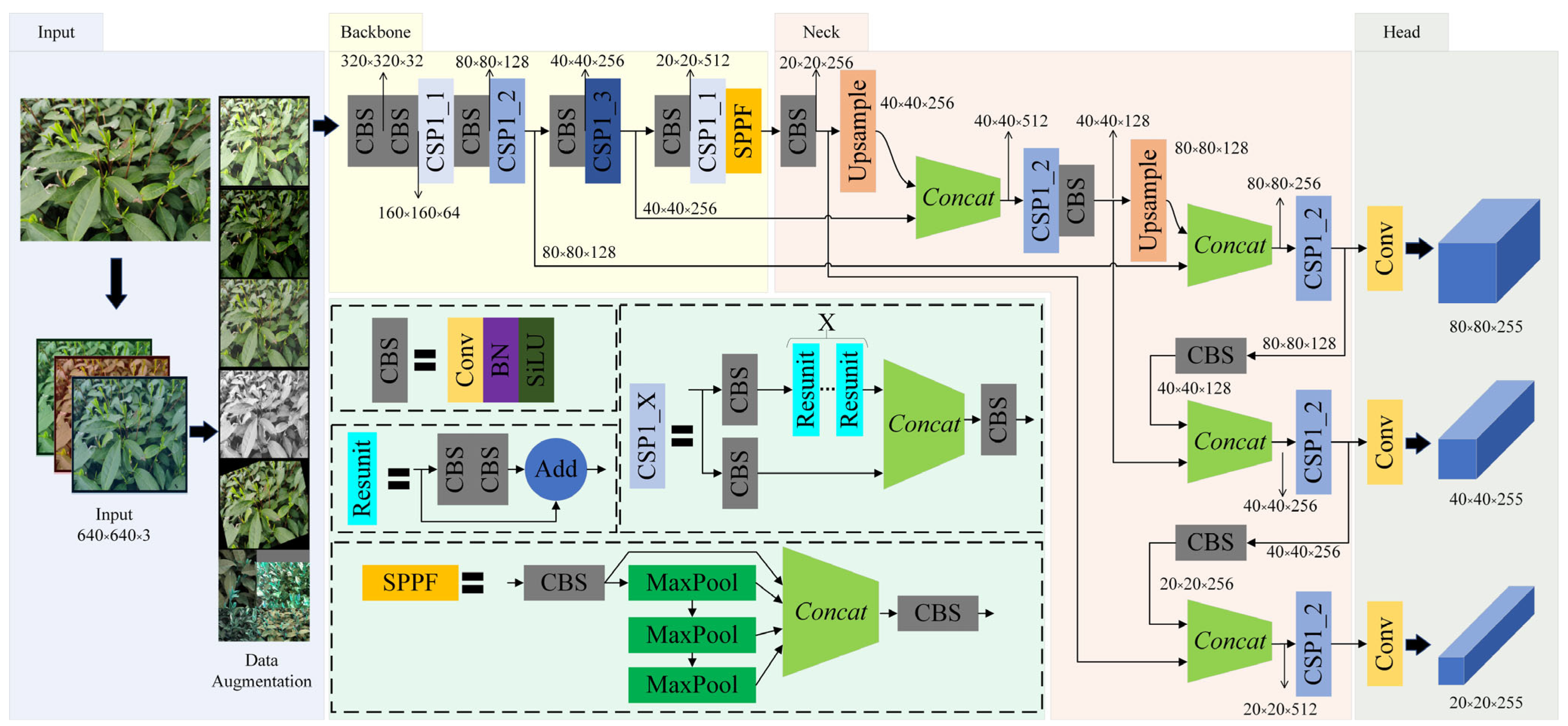
The improved YOLOv5 was developed using Python and based on the original YOLOv5l architecture. The model was trained and tested on Ubuntu 18.04 LTS using an Intel i7-10700 processor, an NVIDIA GeForce RTX 3090, CUDA Version 11.7, PyTorch version 1.8.0, and Python version 3.8. The training process consisted of 700 epochs with a batch size of 64 and an SGD optimizer. The training results are shown in Figure 13. The proposed model achieved its best performance in epoch 473, with a precision of 76.2%, a recall of 77.6%, and an mAP of 82%.
Furthermore, the model was tested on a previously unseen test dataset. The results for precision, recall, and mAP at different confidence levels are shown in Figure 14, with the best mAP of 85.2% achieved at a class ST of 84.8% and a class AT of 85.6%.
Following the training of the proposed model, a comparison was made between its testing results and those of the YOLOv5l model, as detailed in Table 2. The proposed model showed improved performance over YOLOv5l, with higher precision, recall, and mAP scores. Specifically, the mAP of all classes in the proposed model was found to be 3.2% higher than that of YOLOv5l. The ST class of the proposed model showed a 3.7% increase in mAP compared to YOLOv5l, while the AT class of the proposed model showed a 2.7% increase. Moreover, the proposed model had only 60% of the parameters and size of YOLOv5l. The number of FLOPs in the proposed model was only 55% that in YOLOv5l. Furthermore, despite our model having more layers than YOLOv5l, which could limit its performance, the speed of our model on GPU and CPU devices was higher than that of YOLOv5l, and was close to that of YOLOv5m.
Some sample detections performed using both the original and improved models are shown in Figure 15. A yellow circle indicates that the detector missed this target, while a red circle indicates that the detector detected this non-target. It is shown that both the proposed and original methods rarely detected non-targets, and the improved model could detect more small targets in the same scene, demonstrating higher recall.

3.1.3. Ablation Study

An ablation study was conducted to investigate the contribution of individual components or features to the overall performance of the improved model. By systematically removing or disabling different parts of the model and evaluating the resulting performance, insights into the relative importance of each component can be gained, including CAM, BiFPN and GhostConv.
The results of the ablation study are presented and compared in Table 3. The Coordinate Attention Mechanism was found to improve the mAP of the model without significantly increasing the number of parameters and FLOPs. The BiFPN improved the mAP of the model by utilizing multi-scale feature fusion, but it also increased the number of layers and FLOPs. GhostConv reduced the number of parameters and model size to 63% that of the previous version, as well as reducing the number of FLOPs to 55% that of the original. Despite the increase in the number of layers due to DWConv in the GhostConv block, it improved the speed of the model when running on both GPU and CPU devices.

3.1.4. Experimental Comparison with Different Detection Methods

The improved model presented in this paper is compared with other state-of-the-art detection models in Table 4. The results show that the proposed algorithm performed extremely well in terms of detection speed, model size, and computational amount while ensuring the highest mAP. The SSD model, which uses Vgg16 as the backbone network, had a fast detection speed, low computational complexity, and small model size, but low precision. The Faster-RCNN model, which uses Resnet50 as the backbone network, had higher accuracy, but the largest model size and computational amount, and the slowest detection speed. The YOLO series models, including YOLOv3, YOLOv4, YOLOv5, YOLOv6, YOLO7, and YOLOv8l, performed worse than the proposed improved model in terms of mAP, model size, and detection speed. The YOLOv8m and YOLOX models have a model size similar to the proposed algorithm, and these two models performed well in GPU detection speed, both above 90 FPS, but their performance on CPU devices was worse, and their precision scores were lower than that of the proposed model. Overall, the proposed improved object detection model for tea buds had the best performance among those state-of-the-art detection models.

3.2. Experiments on OPVSM

3.2.1. Preparation

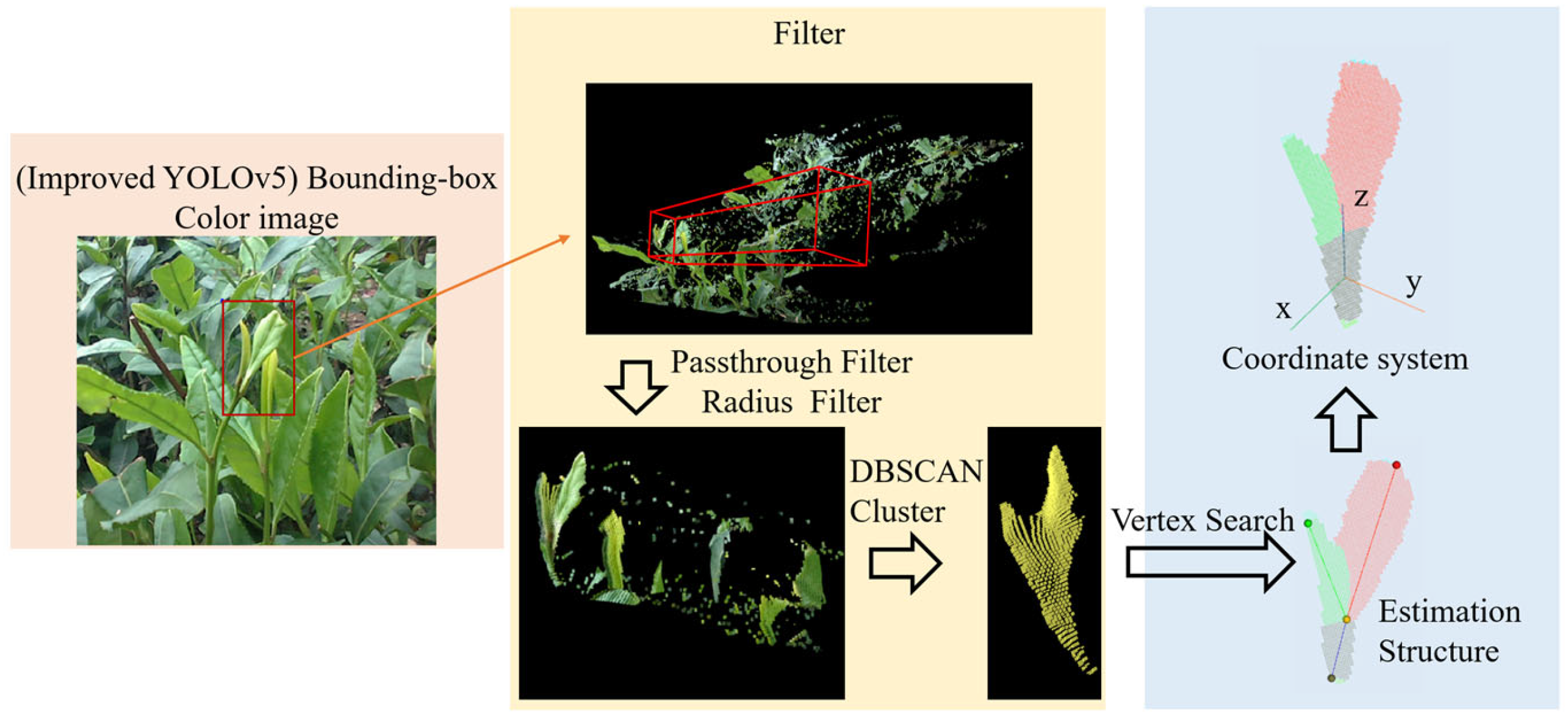
In this paper, the target was set as BL1 (one bud and one leaf). A total of 50 pointclouds including the BL1 target were acquired from the field using a depth camera. As shown in Figure 16, according to the method in Section 2.2.1, each pointcloud was detected using the improved model, filtered by a passthrough filter and a radius filter, clustered using the DBSCAN algorithm, and finally estimated via the OPVSM to build the coordinate system of tea buds.

3.2.2. Results

All pointclouds collected in the field for testing were processed, and the results of the model construction were examined and analyzed. Some of the test results are shown in Figure 17.
After testing, the OPVSM successfully fitted the actual poses of 45 tea buds out of the total samples. The accuracy of this method was around 90%. The wrong results were primarily due to the bad pointclouds and local optima. As shown in Figure 17, the imprecise bounding boxes and measurement instability of the depth camera led to the acquisition of bad pointclouds. Additionally, the search process may have been affected by the initial parameters of the algorithm, resulting in local optima.
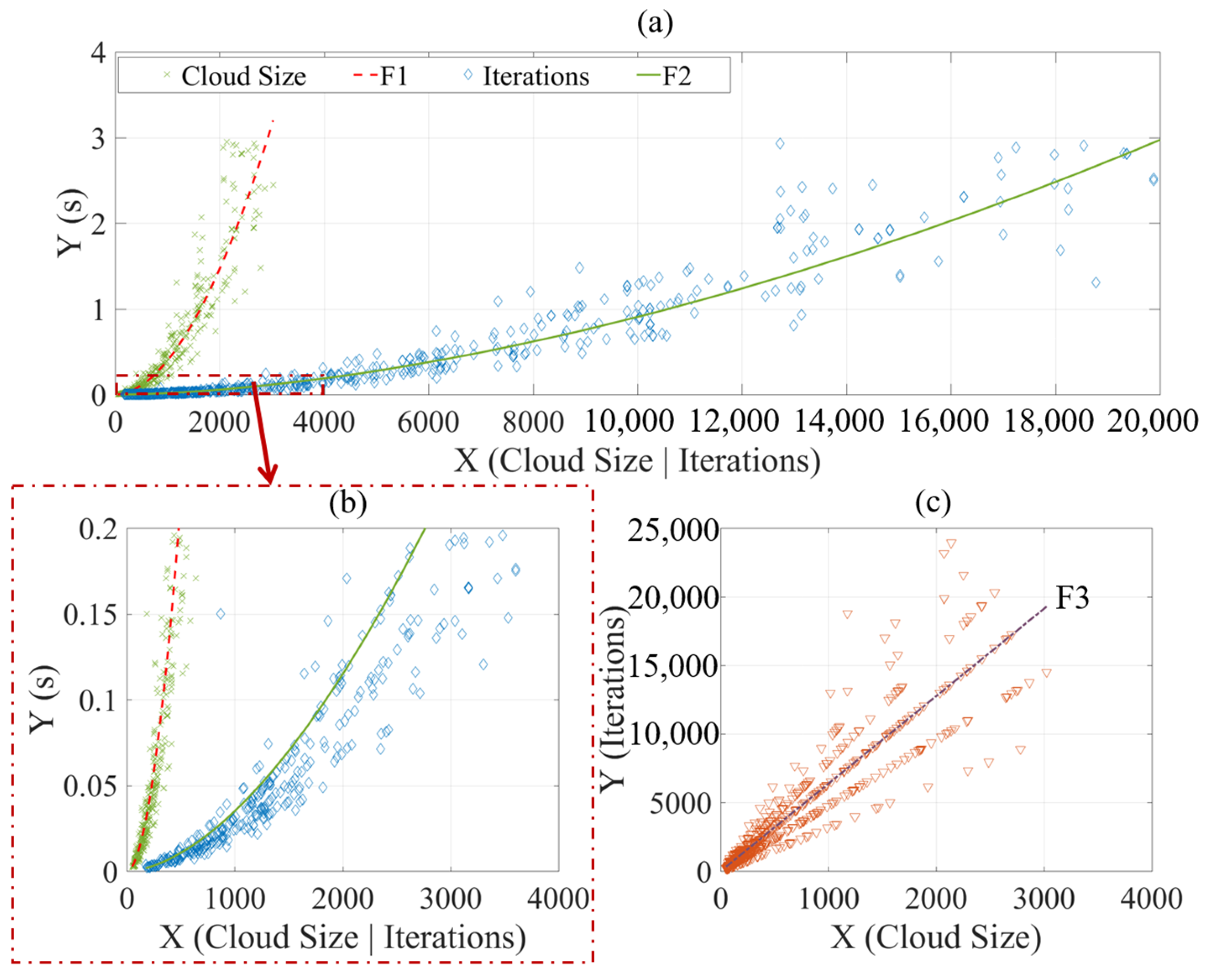
Next, in order to evaluate the performance of the OPVSM, various metrics were recorded during the process, including the pointcloud size, number of iterations, and processing time. To increase the size of test samples, each pointcloud was downsampled multiple times, resulting in a total of 619 test samples, as shown in Figure 18.
As the pointcloud size and number of iterations increase, the processing time also increases exponentially. F1 in Figure 18a represents the fitting curve between pointcloud size and processing times, built using the Levenberg–Marquardt method with a function of f(x) = axb. Similarly, F2 in Figure 18b represents the fitting curve between number of iterations and processing times, built using the same method and function as F1.
Furthermore, Figure 18c shows the proportional relationship between pointcloud size and number of iterations, which could be fitted as a proportional curve (F3). The parameters and evaluation metrics of these fitting curves are shown in Table 5.
The primary independent variable is the cloud size. As the cloud size increases, the number of iterations also increases proportionally, while the processing time increases exponentially. The proportional function (F3) was identified between the cloud size and number of iterations, with a coefficient a of 6.375. Although the SSE and RMSE of this fitting curve were large, indicating that the data points in Figure 18c were scattered, the fitting curve had strong explanatory power and a good fitting result due to a high R-square value of 0.9995.
Notably, the two exponent coefficients, b, in F1 and F2 were close to each other. Additionally, the difference between the two coefficients a in F1 and F2 was 6.98 times, which was close to the coefficient a in F3. The time complexity O(n) of this algorithm is was nearly equal to n1.7~1.9, where n is the size of the pointcloud.
To achieve real-time processing, the process of the proposed algorithm had to be completed within 0.2 s. Thus, in Figure 18b, the plot with processing times of 0 s to 0.2 s was examined. The cloud size should be no larger than 800, and the number of iterations should be no greater than 4000, allowing for a processing time of less than 0.2 s. To reduce the pointcloud size, the voxel filter was used to down-sample the pointcloud to a size of 800. The voxel filter replaced all points within a voxel grid cell with the point closest to the center of the cell, effectively reducing the number of 3D points in the pointcloud while preserving the overall shape of the object being represented. The algorithm results after filtering are shown in Figure 19.
The processing time in Figure 19 includes the voxel filtering process. After voxel filtering with a voxel grid 1 mm × 1 mm × 1 mm in size, the cloud size was reduced to 1/6, the number of iterations was reduced to 1/10, and the processing time was reduced to 1/78, while the pose of the tea buds was correctly built. Furthermore, considering the sparse distribution of the pointcloud along the z axis due to the acquisition principle of the depth camera, we set the voxel grid with a size of 2 mm × 2 mm × 1 mm as the voxel filter, and the cloud size was reduced to 1/17, the number of iterations was reduced to 1/35, the processing time was reduced to 1/618, and the pose of the tea bud was correctly built. This test demonstrated that this method can be applied in real time.

3.3. Discussion

After analyzing the errors in the test dataset, it was found that blurred objects in the image often confused the detector. This was especially true when the camera captured tea buds from a side angle, as the distant buds were also captured in the image. Due to the limited depth of field of the camera, these tea buds were often blurred, making it difficult to manually label all tea buds accurately. As a result, the model was more prone to errors when it encountered these blurred targets. Additionally, the occlusion between the tea buds and illumination (especially overexposure) also led to some mistakes in these detection results. All of these possible factors reduced the precision and recall of this detection model.
There are several ways to address these problems. Firstly, improving the image quality can be achieved by using a better camera or adjusting the illumination conditions to avoid overexposure. Secondly, developing an image processing algorithm combined with a depth camera to segment the distant background and remove blurred targets far away from the camera can be helpful. Additionally, training the model on datasets with images captured from multiple angles may improve its ability to detect objects from different perspectives, thereby reducing the impact of occlusions and improving detection accuracy.
The OPVSM’s performance is affected by bad pointclouds and local optima. The imprecise bounding boxes and measurement instability of the depth camera result in incomplete pointclouds for the tea buds. While some of these incomplete pointclouds still retain the shape of the tea buds, others have their shapes destroyed, making it difficult for the algorithm to operate effectively and increasing the likelihood of it getting stuck in local minima. Combining multiple sensors to fill in missing data or preprocessing the pointclouds to classify and remove low-quality pointclouds may help to solve this problem.
Overall, this research work has several limitations that need to be acknowledged. Firstly, the dataset used in our research, although extensively acquired, annotated, and curated over a period of three years, may not fully capture the diversity of tea buds in real-world scenarios. This limitation could potentially impact the generalizability of our results to unseen data or different settings. To overcome this limitation, future studies could focus on incorporating larger and more diverse datasets to enhance the robustness and applicability of the proposed methods. Secondly, while OPSVM is based on breadth-first search and does not require learning from big data, it is important to validate the method on a larger and more diverse test set to enhance the generalizability of our results. This validation will be conducted in future studies. Furthermore, the proposed methodology and algorithms are subject to computational constraints, and the scalability and computational efficiency of the model may pose challenges when applied in real time or in resource-constrained environments. Addressing these limitations could involve exploring optimization techniques or alternative architectures that improve efficiency without compromising performance. Lastly, this study primarily focused on tea bud detection in the field as a specific application domain. The effectiveness of the proposed approach in other locations, such as laboratory or greenhouse settings, or for detecting other small targets, remains an open question. Further investigations and experiments are necessary to evaluate the generalizability of our findings and determine the suitability of the proposed approach in diverse contexts.

4. Conclusions

In conclusion, an algorithm for detecting and estimating the pose of tea buds using a depth camera was proposed in this paper. The improved YOLOv5l model with CAM, BiFPN and GhostConv components demonstrated superior performance in detecting tea buds, achieving a higher mAP of 85.2%, a faster speed of 87.71 FPS on GPU devices and 6.88 FPS on CPU devices, a lower parameter value of 29.25 M, and a lower FLOP value of 59.8 G compared with other models. Moreover, the datasets were collected under different conditions and were augmented to enhance the model’s generalization ability under complex scenes. The OPVSM achieved results with 90% accuracy during testing. It builds a graph model that fits the tea buds by iteratively searching for the best vertices from the point cloud guided by a loss function. The algorithm gradually improves the fitness of the model until it reaches a local minimum. The optimal vertex set V acquired could build a graph model that accurately represents the pose of the tea bud. This approach is adaptive to variations in size, color, and shape features. The algorithm’s time complexity O(n) is n1.7~1.9, and it can be completed within 0.2 s by using voxel filtering to compress the pointcloud to around 800.
The combination of the proposed detection model and the OPVSM resulted in a reliable and efficient approach for tea bud detection and pose estimation. This study has the potential to be used in tea picking automation and can be extended to other crops and objects for precision agriculture and robotic applications. Future work will aim to improve the model performance and inference speed via data cleaning and expansion, model pruning and compression, and other methods, and parallel processing will be used to accelerate the OPVSM.

Author Contributions

Conceptualization, Z.C., J.C., Y.L., Z.G. and T.Y.; methodology, Z.C.; software, Z.C.; validation, Z.C., Z.G. and T.Y.; formal analysis, Z.C.; investigation, Z.C., Z.G. and T.Y.; resources, Z.C., J.C. and Y.L.; data curation, Z.C. and J.C.; writing—original draft preparation, Z.C.; writing—review and editing, Z.C. and Y.L.; visualization, Z.C.; supervision, J.C.; project administration, J.C.; funding acquisition, J.C. All authors have read and agreed to the published version of the manuscript.

Funding

This research was funded by “Leading Goose” R&D Program of Zhejiang (grant number: 2022C02052) and the National Natural Science Foundation of China (Grant No. 51975537).

Institutional Review Board Statement

Not applicable.

Informed Consent Statement

Not applicable.

Data Availability Statement

The data presented in this study are available on request from the corresponding author. The data are not publicly available due to confidentiality restrictions.

Acknowledgments

The authors deeply appreciate the Tea Research Institute, Chinese Academy of Agricultural Sciences for their assistance in conducting field experiments.

Conflicts of Interest

The authors declare no conflict of interest.

References

  1. Chen, J.; Chen, Y.; Jin, X.; Che, J.; Gao, F.; Li, N. Research on a Parallel Robot for Tea Flushes Plucking; Atlantis Press: Amsterdam, The Netherlands, 2015; pp. 22–26. [Google Scholar]
  2. Yang, H.; Chen, L.; Ma, Z.; Chen, M.; Zhong, Y.; Deng, F.; Li, M. Computer Vision-Based High-Quality Tea Automatic Plucking Robot Using Delta Parallel Manipulator. Comput. Electron. Agric. 2021, 181, 105946. [Google Scholar] [CrossRef]
  3. Zhang, H.; Chen, Y.; Wang, W.; Zhang, G. Positioning Method for Tea Picking Using Active Computer Vision. Trans. Chin. Soc. Agric. Mach. 2014, 45, 61–65+78. [Google Scholar]
  4. Zhang, L.; Zou, L.; Wu, C.; Jia, J.; Chen, J. Method of Famous Tea Sprout Identification and Segmentation Based on Improved Watershed Algorithm. Comput. Electron. Agric. 2021, 184, 106108. [Google Scholar] [CrossRef]
  5. Wu, X.; Zhang, F.; Lv, J. Research on Recognition of Tea Tender Leaf Based on Image Color Information. J. Tea Sci. 2013, 33, 584–589. [Google Scholar] [CrossRef]
  6. Lyu, S.; Chang, M.-C.; Du, D.; Li, W.; Wei, Y.; Coco, M.D.; Carcagnì, P.; Schumann, A.; Munjal, B.; Dang, D.-Q.-T.; et al. UA-DETRAC 2018: Report of AVSS2018 & IWT4S Challenge on Advanced Traffic Monitoring. In Proceedings of the 2018 15th IEEE International Conference on Advanced Video and Signal Based Surveillance (AVSS), Auckland, New Zealand, 27–30 November 2018; pp. 1–6. [Google Scholar]
  7. Zhang, J.; Huang, M.; Jin, X.; Li, X. A Real-Time Chinese Traffic Sign Detection Algorithm Based on Modified YOLOv2. Algorithms 2017, 10, 127. [Google Scholar] [CrossRef] [Green Version]
  8. Zhang, S.; Benenson, R.; Schiele, B. CityPersons: A Diverse Dataset for Pedestrian Detection. arXiv 2017, arXiv:1702.05693. [Google Scholar]
  9. Cui, M.; Lou, Y.; Ge, Y.; Wang, K. LES-YOLO: A Lightweight Pinecone Detection Algorithm Based on Improved YOLOv4-Tiny Network. Comput. Electron. Agric. 2023, 205, 107613. [Google Scholar] [CrossRef]
  10. Zeng, T.; Li, S.; Song, Q.; Zhong, F.; Wei, X. Lightweight Tomato Real-Time Detection Method Based on Improved YOLO and Mobile Deployment. Comput. Electron. Agric. 2023, 205, 107625. [Google Scholar] [CrossRef]
  11. Ma, J.; Lu, A.; Chen, C.; Ma, X.; Ma, Q. YOLOv5-Lotus an Efficient Object Detection Method for Lotus Seedpod in a Natural Environment. Comput. Electron. Agric. 2023, 206, 107635. [Google Scholar] [CrossRef]
  12. Wang, D. Channel Pruned YOLO V5s-Based Deep Learning Approach for Rapid and Accurate Apple Fruitlet Detection before Fruit Thinning. Biosyst. Eng. 2021, 210, 271–281. [Google Scholar] [CrossRef]
  13. Sozzi, M.; Cantalamessa, S.; Cogato, A.; Kayad, A.; Marinello, F. Automatic Bunch Detection in White Grape Varieties Using YOLOv3, YOLOv4, and YOLOv5 Deep Learning Algorithms. Agronomy 2022, 12, 319. [Google Scholar] [CrossRef]
  14. Cardellicchio, A.; Solimani, F.; Dimauro, G.; Petrozza, A.; Summerer, S.; Cellini, F.; Renò, V. Detection of Tomato Plant Phenotyping Traits Using YOLOv5-Based Single Stage Detectors. Comput. Electron. Agric. 2023, 207, 107757. [Google Scholar] [CrossRef]
  15. Murthi, M.; Thangavel, S.K. A Semi-Automated System for Smart Harvesting of Tea Leaves; IEEE: Banglore, India, 2017; pp. 1–10. [Google Scholar]
  16. Chen, B.; Yan, J.; Wang, K. Fresh Tea Sprouts Detection via Image Enhancement and Fusion SSD. J. Control Sci. Eng. 2021, 2021, 6614672. [Google Scholar] [CrossRef]
  17. Xu, W.; Zhao, L.; Li, J.; Shang, S.; Ding, X.; Wang, T. Detection and Classification of Tea Buds Based on Deep Learning. Comput. Electron. Agric. 2022, 192, 106547. [Google Scholar] [CrossRef]
  18. Gui, Z.; Chen, J.; Li, Y.; Chen, Z.; Wu, C.; Dong, C. A Lightweight Tea Bud Detection Model Based on Yolov5. Comput. Electron. Agric. 2023, 205, 107636. [Google Scholar] [CrossRef]
  19. Hu, G.; Li, S.; Wan, M.; Bao, W. Semantic Segmentation of Tea Geometrid in Natural Scene Images Using Discriminative Pyramid Network. Appl. Soft Comput. 2021, 113, 107984. [Google Scholar] [CrossRef]
  20. Qian, C.; Li, M.; Ren, Y. Tea Sprouts Segmentation via Improved Deep Convolutional Encoder-Decoder Network. IEICE Trans. Inf. Syst. 2020, 103, 476–479. [Google Scholar] [CrossRef] [Green Version]
  21. Chen, Y.-T.; Chen, S.-F. Localizing Plucking Points of Tea Leaves Using Deep Convolutional Neural Networks. Comput. Electron. Agric. 2020, 171, 105298. [Google Scholar] [CrossRef]
  22. Wang, T.; Zhang, K.; Zhang, W.; Wang, R.; Wan, S.; Rao, Y.; Jiang, Z.; Gu, L. Tea Picking Point Detection and Location Based on Mask-RCNN. Inf. Process. Agric. 2021, 10, 267–275. [Google Scholar] [CrossRef]
  23. Li, Y.; He, L.; Jia, J.; Lv, J.; Chen, J.; Qiao, X.; Wu, C. In-Field Tea Shoot Detection and 3D Localization Using an RGB-D Camera. Comput. Electron. Agric. 2021, 185, 106149. [Google Scholar] [CrossRef]
  24. Li, Y.; Wu, S.; He, L.; Tong, J.; Zhao, R.; Jia, J.; Chen, J.; Wu, C. Development and Field Evaluation of a Robotic Harvesting System for Plucking High-Quality Tea. Comput. Electron. Agric. 2023, 206, 107659. [Google Scholar] [CrossRef]
  25. Chen, C.; Lu, J.; Zhou, M.; Yi, J.; Liao, M.; Gao, Z. A YOLOv3-Based Computer Vision System for Identification of Tea Buds and the Picking Point. Comput. Electron. Agric. 2022, 198, 107116. [Google Scholar] [CrossRef]
  26. Han, K.; Wang, Y.; Tian, Q.; Guo, J.; Xu, C.; Xu, C. GhostNet: More Features from Cheap Operations. arXiv 2020, arXiv:1911.11907. [Google Scholar]
  27. Hou, Q.; Zhou, D.; Feng, J. Coordinate Attention for Efficient Mobile Network Design. arXiv 2021, arXiv:2103.02907. [Google Scholar]
  28. Tan, M.; Pang, R.; Le, Q.V. EfficientDet: Scalable and Efficient Object Detection. In Proceedings of the 2020 IEEE/CVF Conference on Computer Vision and Pattern Recognition (CVPR), Seattle, WA, USA, 13–19 June 2020; pp. 10778–10787. [Google Scholar]
  29. Jocher, G.; Chaurasia, A.; Stoken, A.; Borovec, J.; NanoCode012; Kwon, Y.; Michael, K.; Xie, T.; Fang, J.; Imyhxy; et al. Ultralytics/Yolov5: V7.0—YOLOv5 SOTA Realtime Instance Segmentation. Zenodo 2022. [Google Scholar] [CrossRef]
  30. Ester, M.; Kriegel, H.-P.; Xu, X. A Density-Based Algorithm for Discovering Clusters in Large Spatial Databases with Noise. Kdd-96 Proceeding. 1996, pp. 226–231. Available online: https://cdn.aaai.org/KDD/1996/KDD96-037.pdf (accessed on 5 June 2023).
  31. Shorten, C.; Khoshgoftaar, T.M. A Survey on Image Data Augmentation for Deep Learning. J. Big Data 2019, 6, 60. [Google Scholar] [CrossRef] [Green Version]
  32. Bochkovskiy, A.; Wang, C.; Liao, H.M. YOLOv4: Optimal Speed and Accuracy of Object Detection. arXiv 2020, arXiv:2004.10934. [Google Scholar]
Figure 1. Structure of the YOLOv5 model.
Agriculture 13 01405 g001
Figure 2. Architecture of the improved YOLOv5.
Agriculture 13 01405 g002
Figure 3. Structure of the Coordinate Attention Mechanism.
Agriculture 13 01405 g003
Figure 4. Structure of the BiFPN.
Agriculture 13 01405 g004
Figure 5. The GhostConv block.
Agriculture 13 01405 g005
Figure 6. Obtaining the pointcloud of tea bud from the depth camera. (a) Tea bud detected in image; (b) Pointcloud extracted from a depth camera using a passthrough filter; (c) Pointcloud of a tea bud extracted from pervious pointcloud using DBSCAN.
Agriculture 13 01405 g006
Figure 7. The geometry features of the tea buds.
Agriculture 13 01405 g007
Figure 8. Flowchart of the vertex search algorithm.
Agriculture 13 01405 g008
Figure 9. Flowchart of the loss function calculation process.
Agriculture 13 01405 g009
Figure 10. Variety of samples in the dataset.
Agriculture 13 01405 g010
Figure 11. Data augmentation.
Agriculture 13 01405 g011
Figure 12. An example of a mosaic image.
Agriculture 13 01405 g012
Figure 13. Training results of the proposed model.
Agriculture 13 01405 g013
Figure 14. Testing results of the proposed model.
Agriculture 13 01405 g014
Figure 15. Comparison of detection results on images between YOLOv5l and the proposed model.
Agriculture 13 01405 g015
Figure 16. The tea bud pose estimation process.
Agriculture 13 01405 g016
Figure 17. Samples of algorithm-processed images.
Agriculture 13 01405 g017
Figure 18. The performance plots of the proposed algorithm. (a) The impact graph of cloud size and iteration times on processing time; (b) The impact graph of cloud size and iteration times on processing time within 0.2s; (c) The impact graph of cloud size on iteration times.
Agriculture 13 01405 g018
Figure 19. Test results after voxel filtering.
Agriculture 13 01405 g019
Table 1. The performance of different original Yolov5 models for our data.
ModelDepth MultipleWidth
Multiple
mAP (%)Params (M)FLOPs (G)Speed (FPS)
GPU
Speed (FPS)
CPU
Size (M)
YOLOv5x1.331.2581.186.18203.851.541.69165.10
YOLOv5l1182.246.11107.782.643.888.55
YOLOv5m0.670.7581.420.8647.990.095.8440.25
YOLOv5s0.330.578.17.0215.8112.3613.3513.75
Table 2. Comparative experiments between improved and original models.
ModelClassP (%)R (%)mAP (%)Params (M)FLOPs (G)Speed (FPS)
GPU
Speed (FPS)
CPU
Size (M)Layers
YOLOv5lST76.376.381.146.11107.782.643.8184.44367
AT76.680.782.9
All76.578.582
OursST78.478.784.829.2559.887.716.88112.05624
AT7883.585.6
All78.281.185.2
Table 3. Comparison of ablation study results.
ModelmAP (%)Params (M)FLOPs (G)Speed (FPS)
GPU
Speed (FPS)
CPU
Size (M)Layers
YOLOv5l8246.11107.782.643.8184.44367
YOLOv5l + CAM8446.13107.781.33.77184.52377
YOLOv5l + BiFPN8346.37108.581.33.72185.48367
YOLOv5l + CAM + BiFPN84.446.4108.677.53.29185.6377
YOLOv5l + CAM + BiFPN
+ GhostConv
85.229.2559.887.716.88112.05624
Table 4. Comparison between different object detection methods.
ModelmAP (%)Params (M)FLOPs (G)Speed (FPS)
GPU
Speed (FPS)
CPU
Size (M)
Vgg16-SSD67.1826.1562.884.264.82104.6
Resnet50-Faster-RCNN80.05137.07370.4112.091.03548.28
YOLOv3-SPP82.462.55155.476.923.08250.2
CSP-YOLOv4-Mish80.1126.67177.749.751.91242.67
YOLOv58246.11107.778.742.77184.44
YOLOR74.652.49119.373.532.89100.61
YOLOv679.259.54150.544.823.43114.19
YOLOv776.636.48103.275.192.6371.35
YOLOv8m81.825.8478.7935.66103.36
YOLOv8l81.143.61164.876.343.05174.44
YOLOX82.323.2762.195.235.3593.08
Ours85.229.2559.887.716.88112.05
Table 5. Parameters and metrics of fitting curves.
CurveFunctionabSSER-SquareRMSE
F1f(x) = axb1.71 × 10−61.8890.88410.99920.03785
F2f(x) = axb2.45 × 10−71.7170.72450.99940.03427
F3f(x) = ax6.375\8,052,0000.9995114.1
Disclaimer/Publisher’s Note: The statements, opinions and data contained in all publications are solely those of the individual author(s) and contributor(s) and not of MDPI and/or the editor(s). MDPI and/or the editor(s) disclaim responsibility for any injury to people or property resulting from any ideas, methods, instructions or products referred to in the content.

