


Research on the Control Strategy of Leafy Vegetable Harvester Travel Speed Automatic Control System
 , ,
, ,
Abstract
:1. Introduction
2. Materials and Methods
2.1. Machine Structure and Working Principle
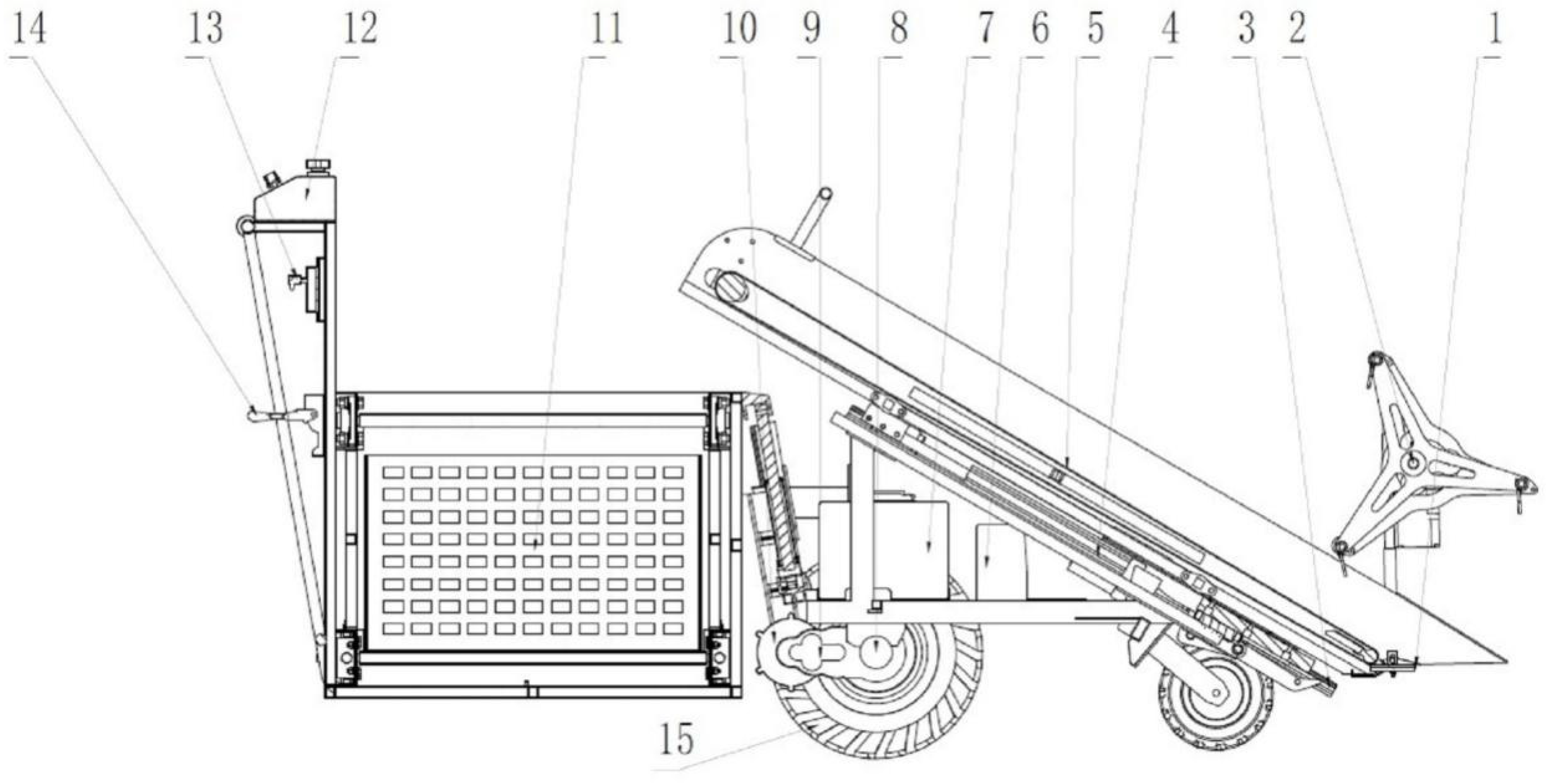
2.1.1. Machine Structure and Technical Parameters
2.1.2. Working Principle
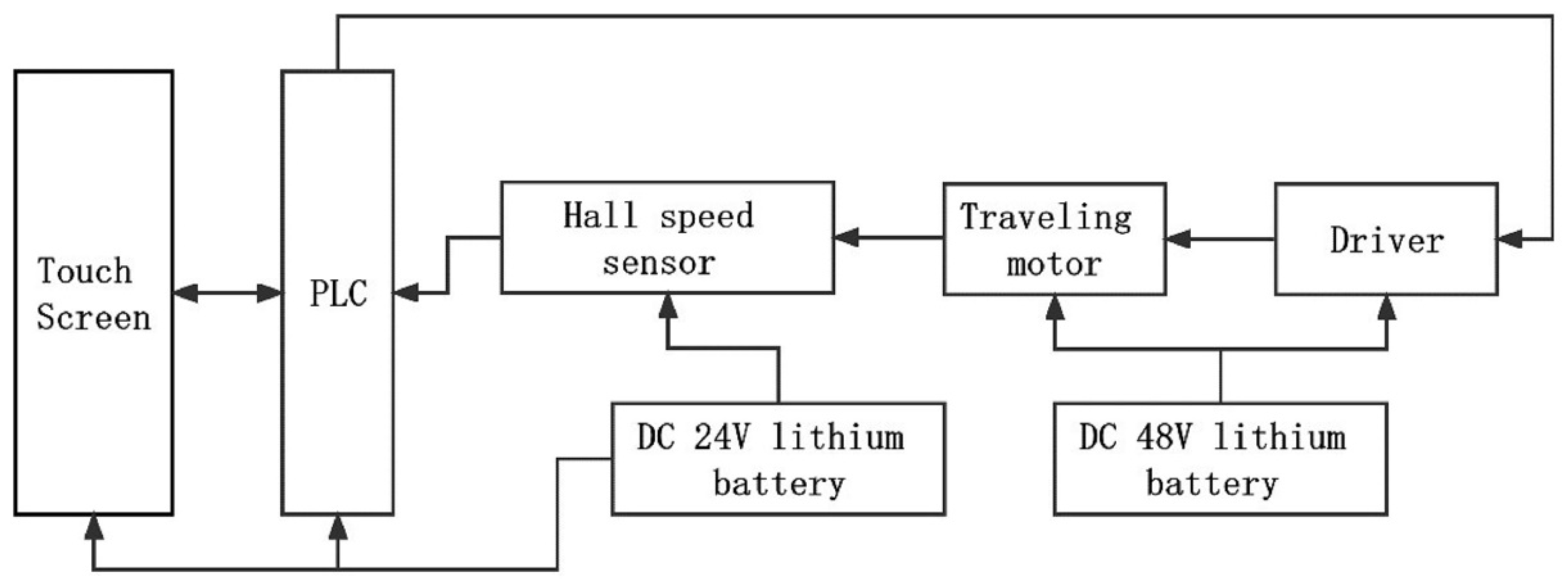
2.2. Travel Speed Automatic Control System Components
2.3. Model of the Travel Drive System
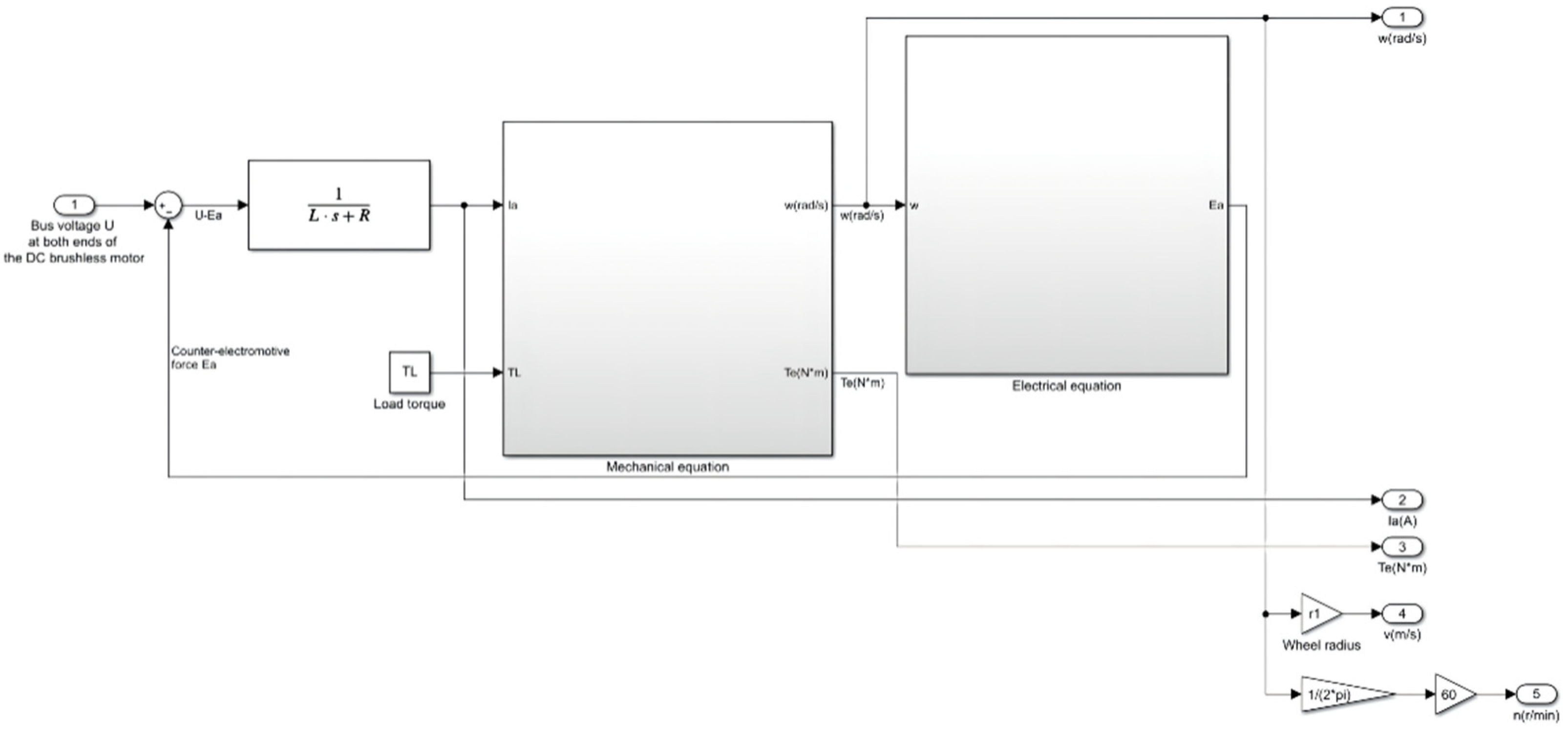
2.3.1. Model of the Travel Drive Motor
2.3.2. Drive Train Model
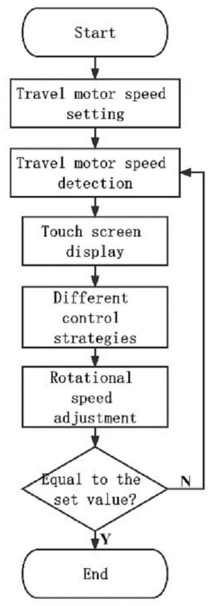
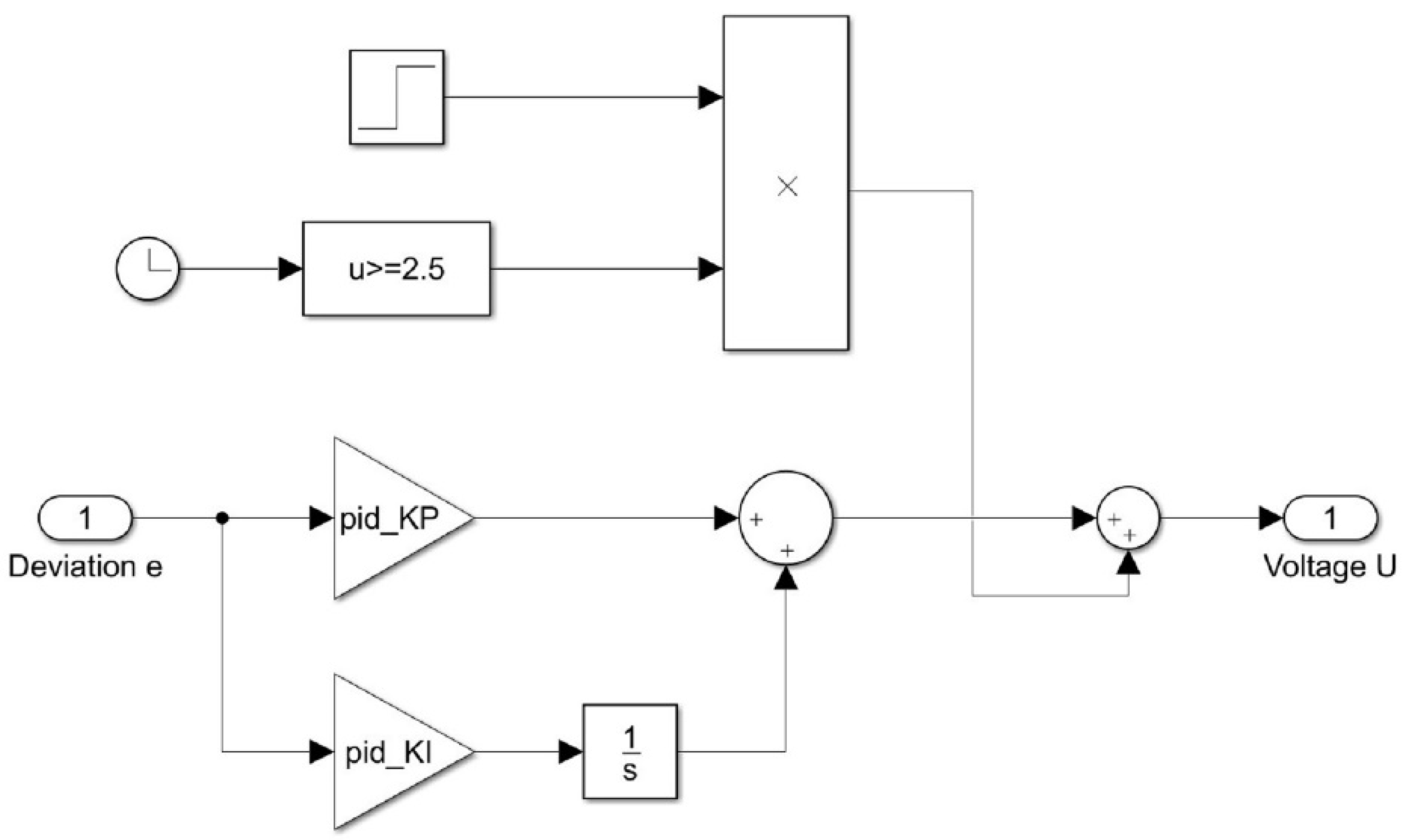
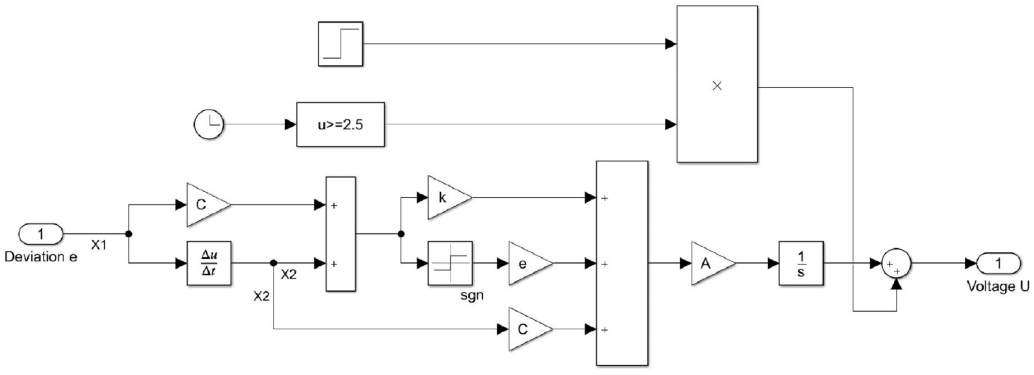
2.4. Control Strategy Establishment
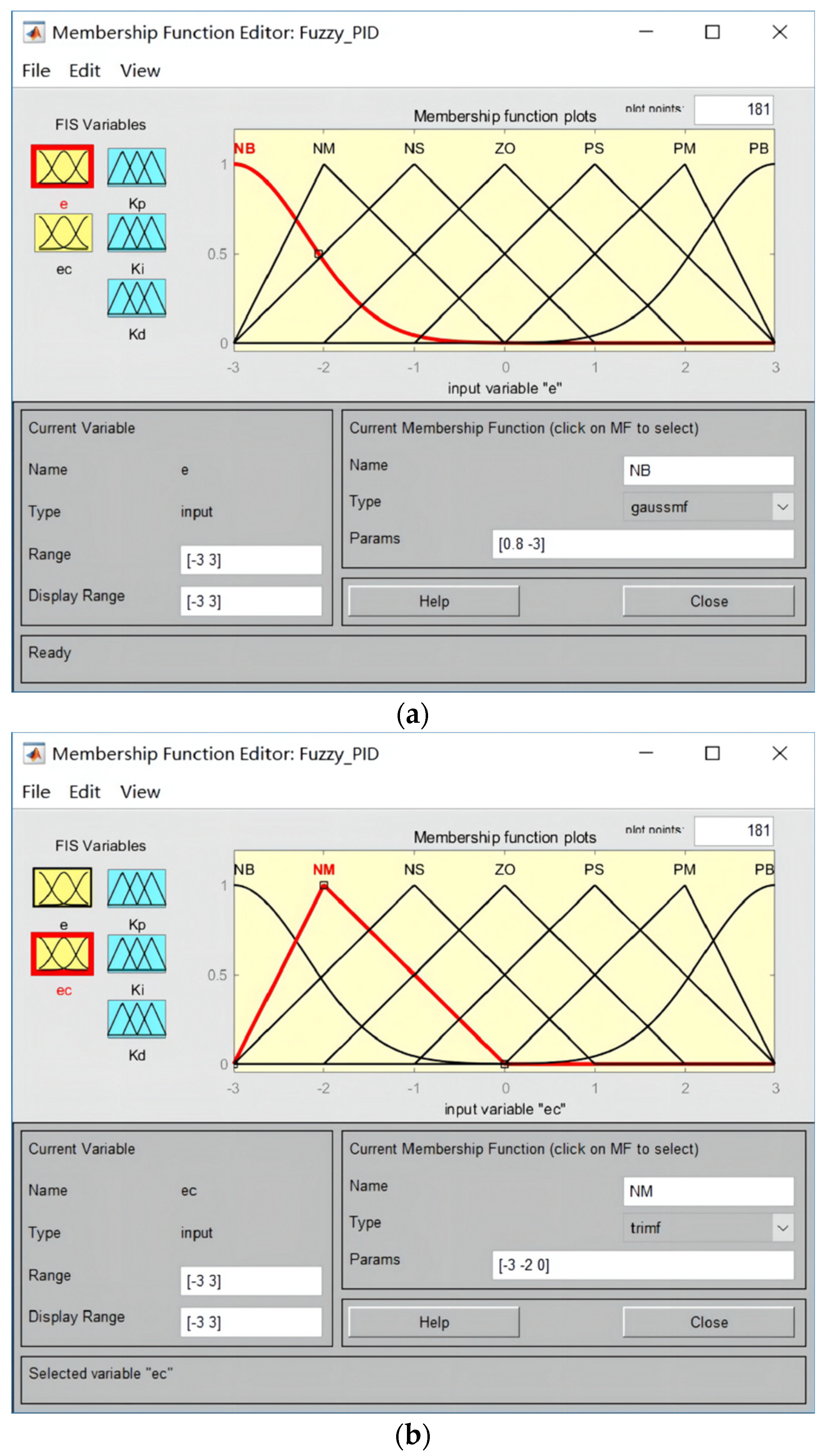
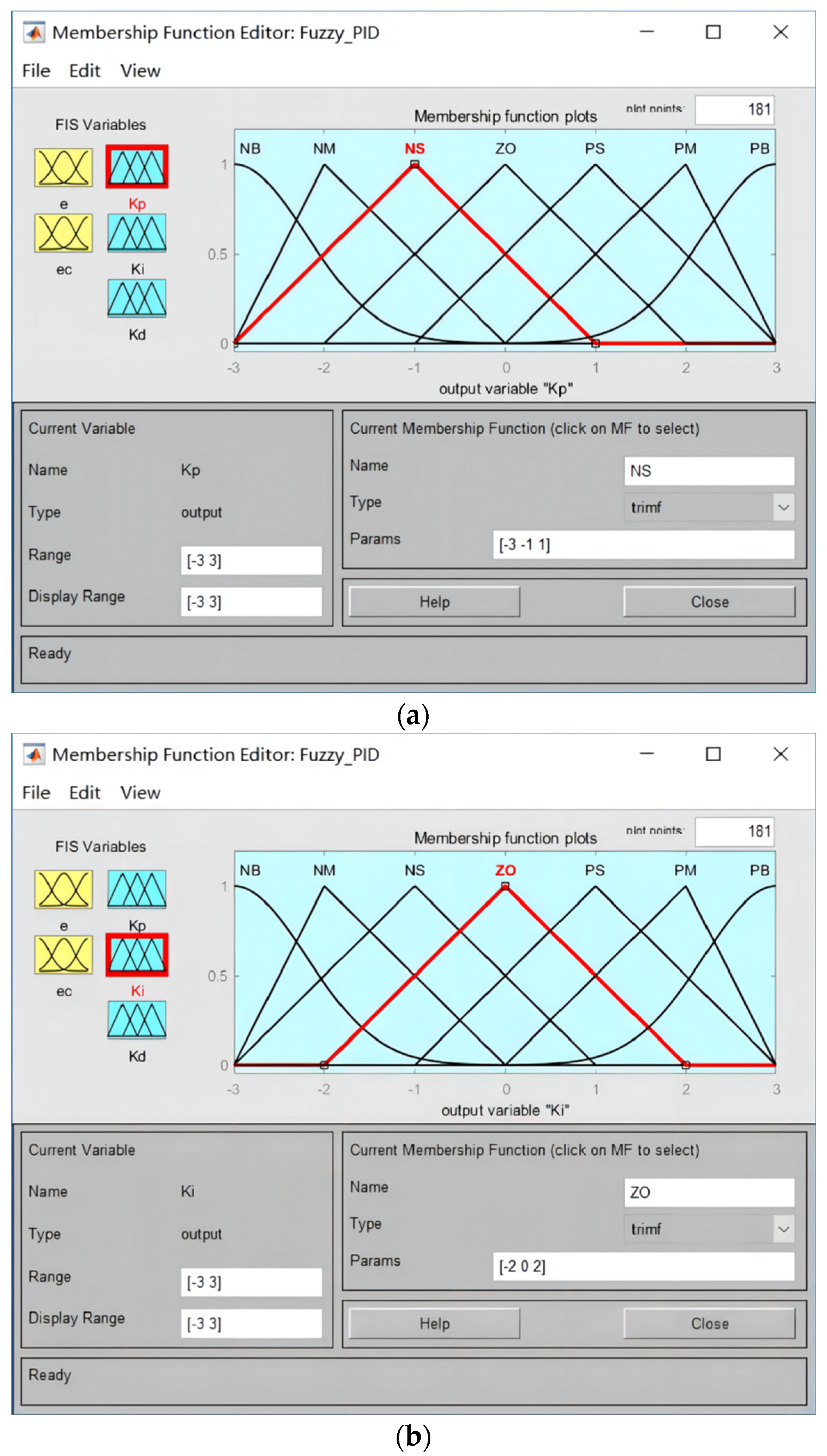
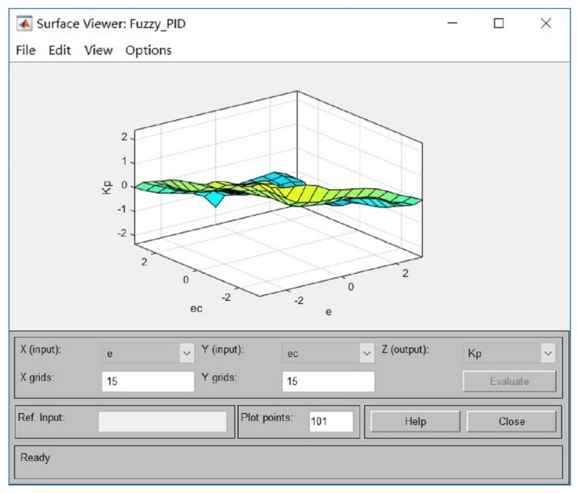
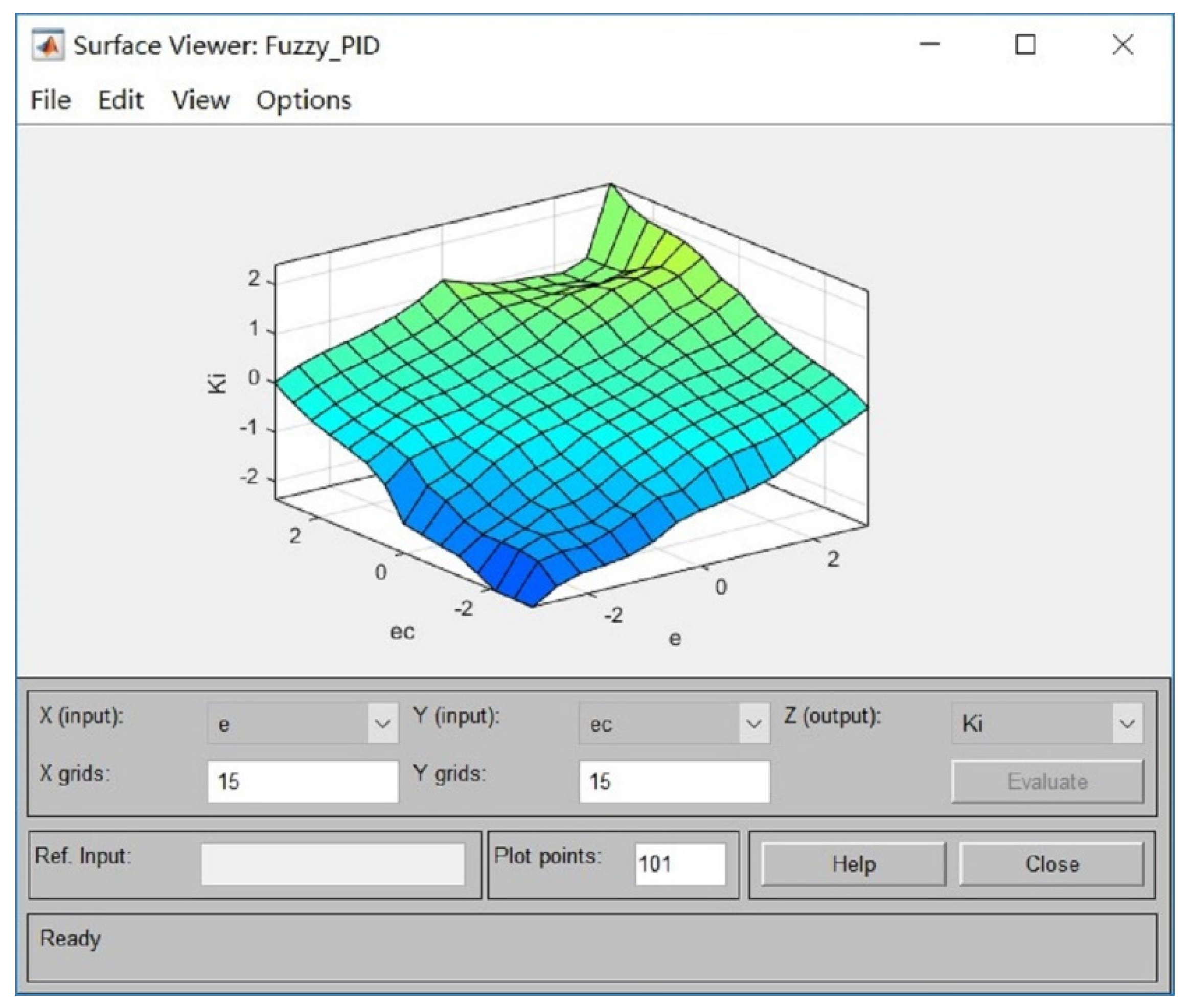
2.4.1. Adaptive Fuzzy PID Control Strategy Establishment
2.4.2. Sliding Mode Control Strategy Establishment
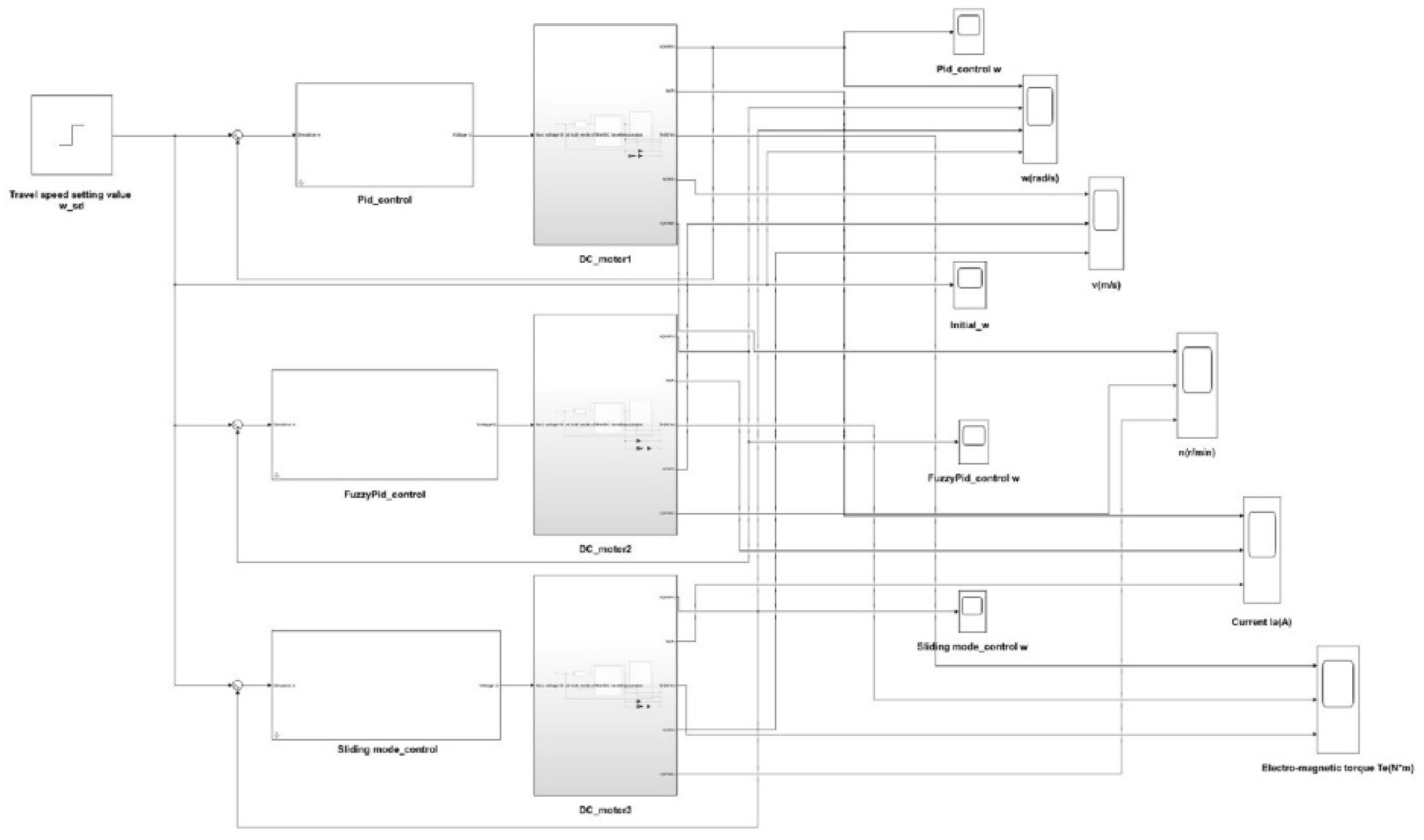
2.5. Control Model Building and Simulation
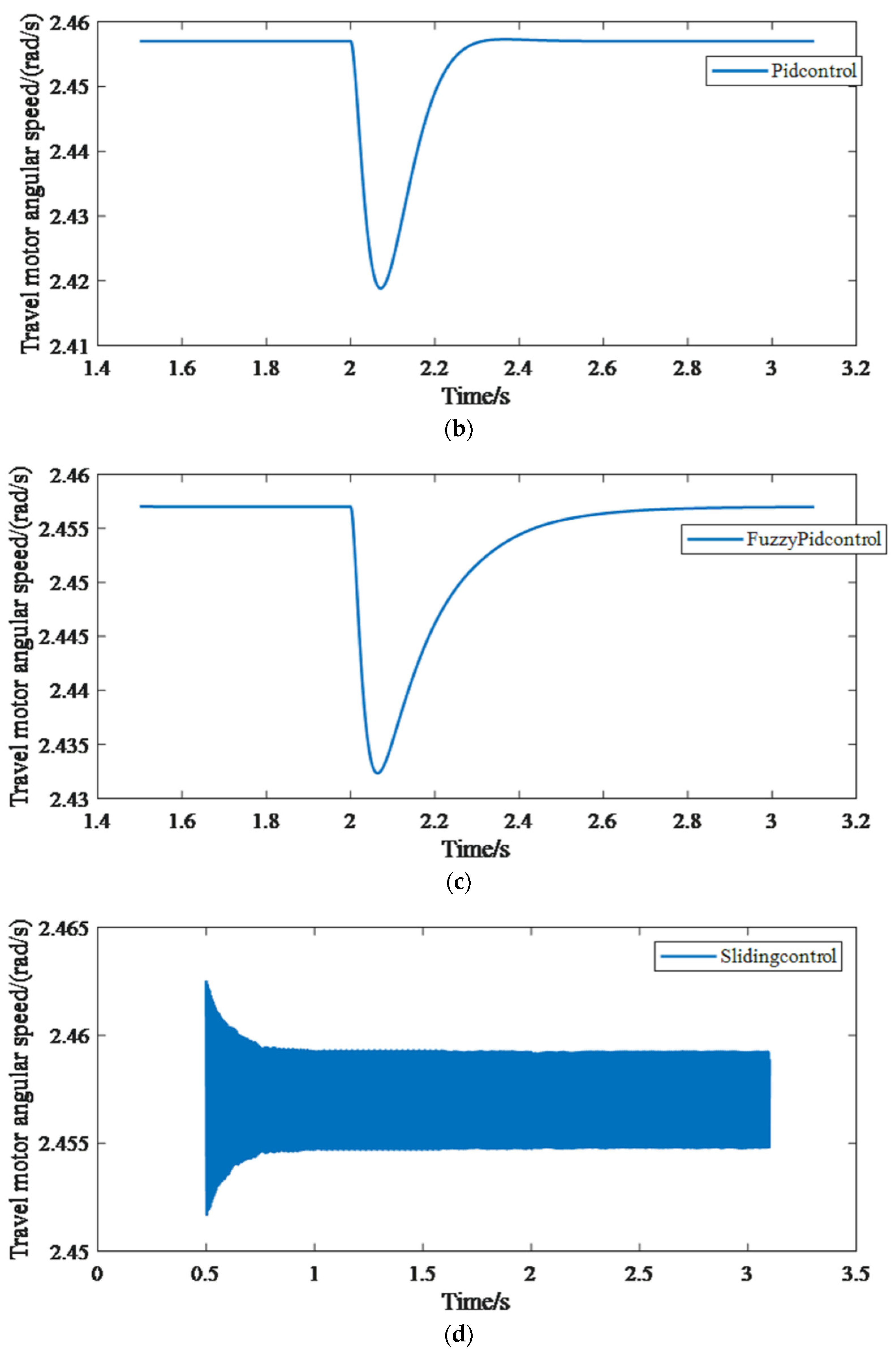
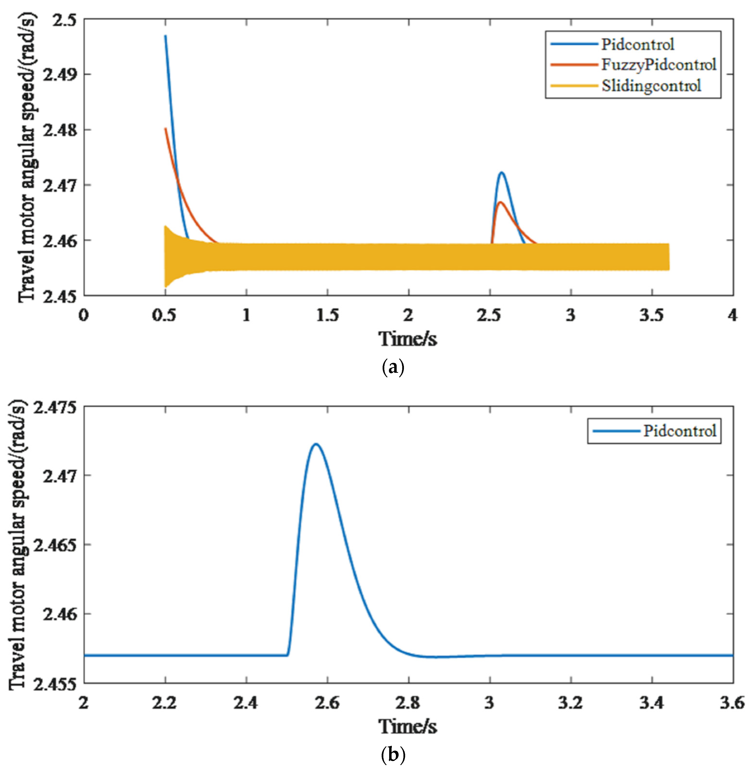
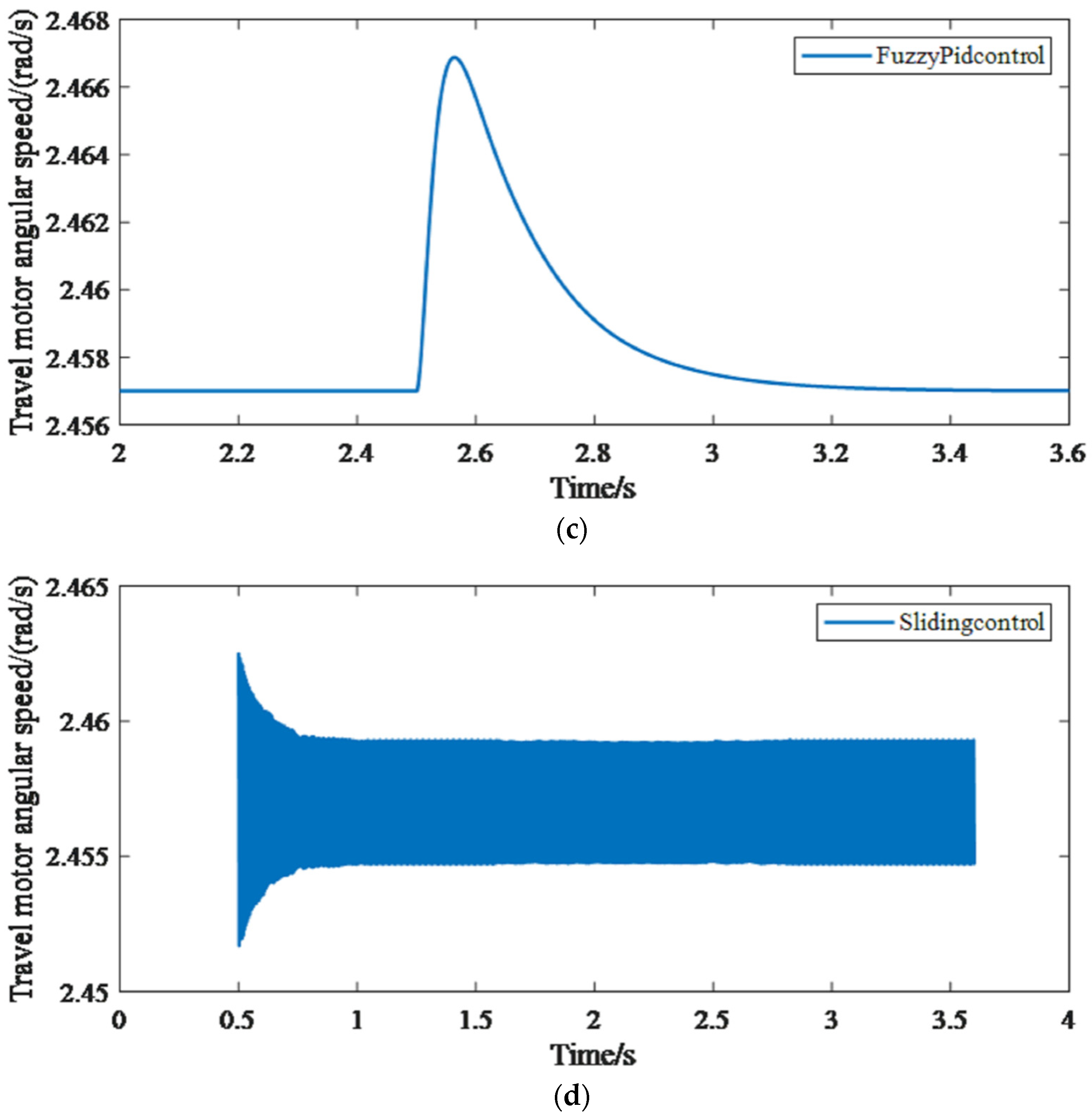
3. Results
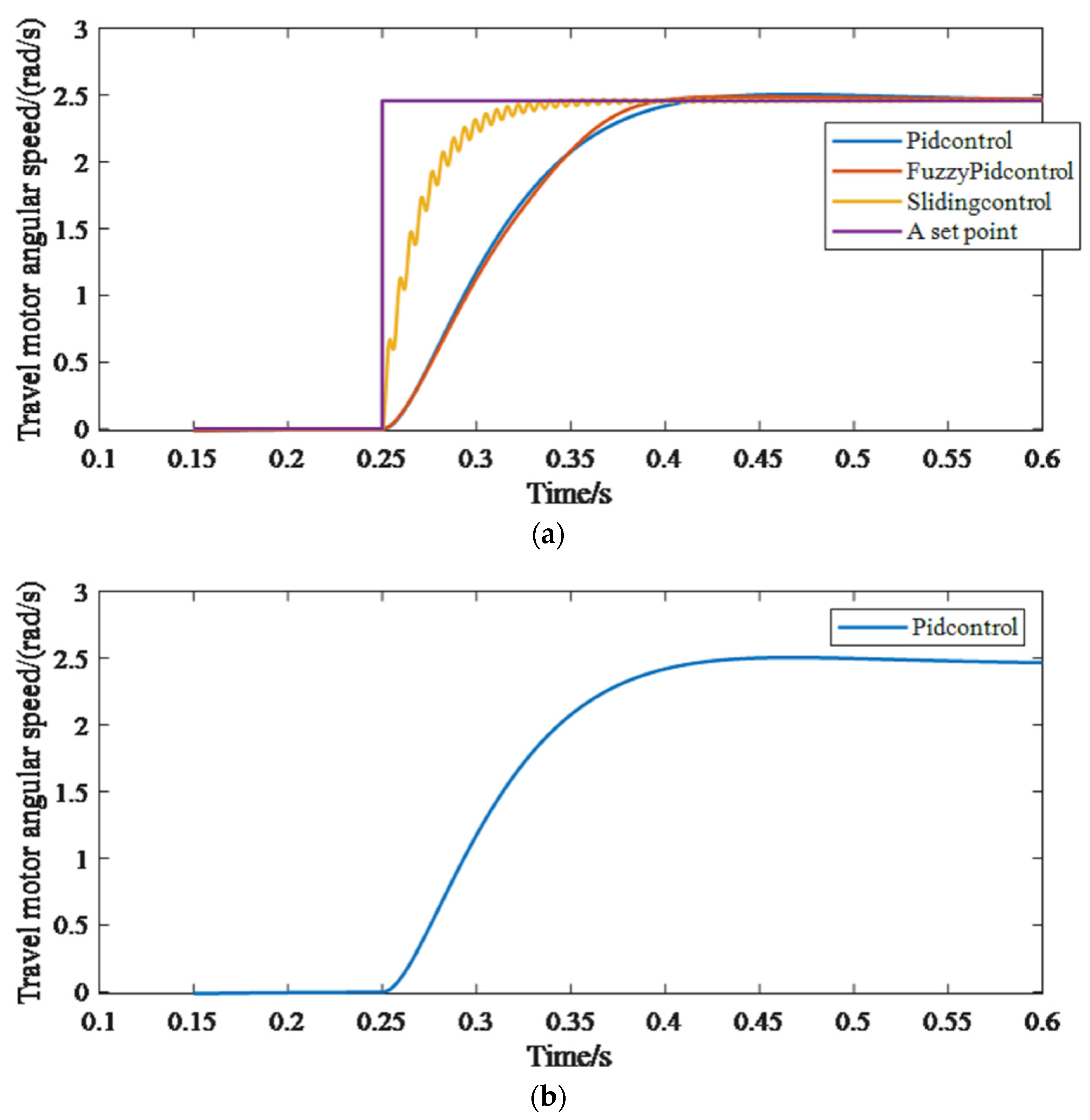
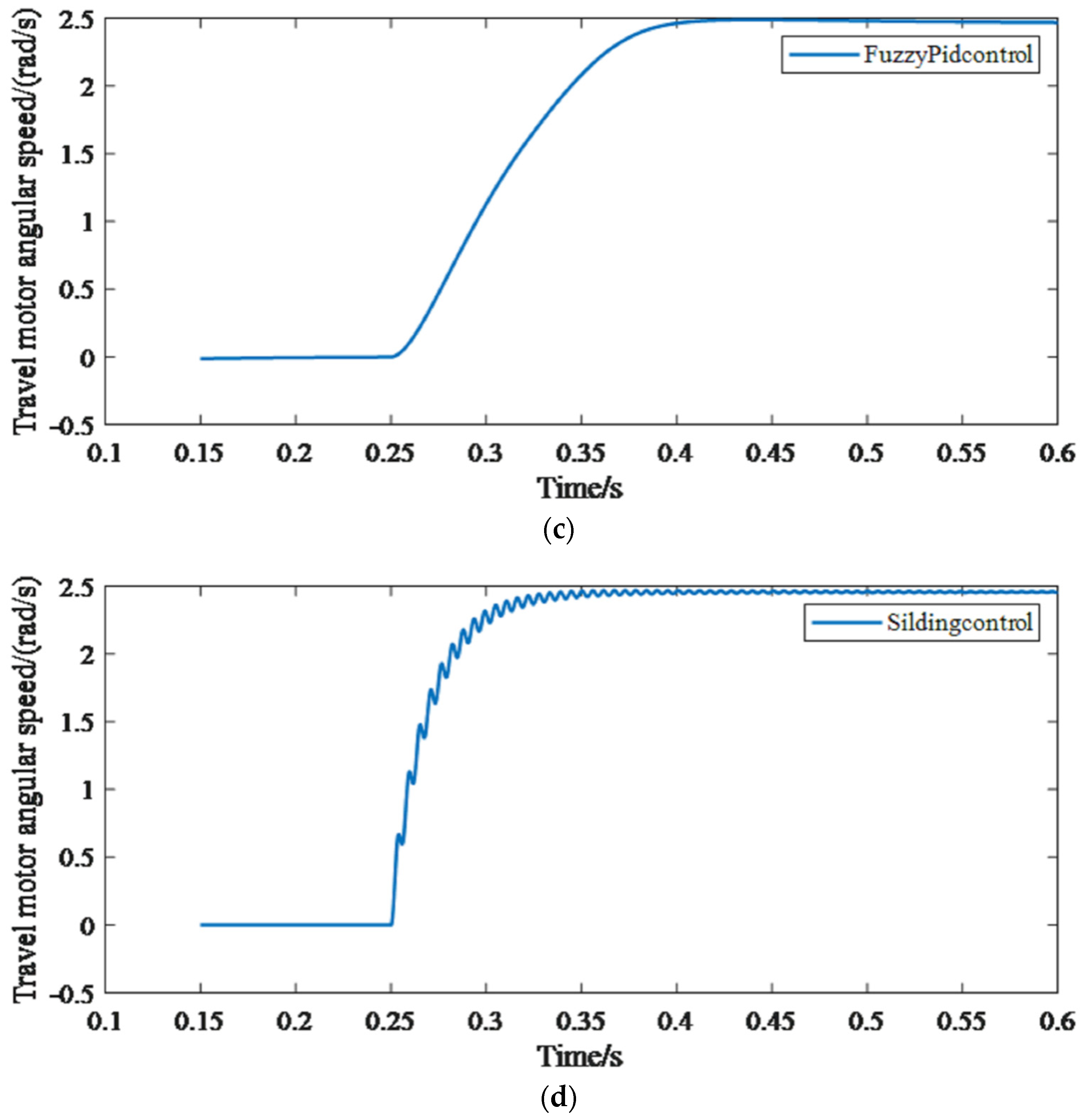
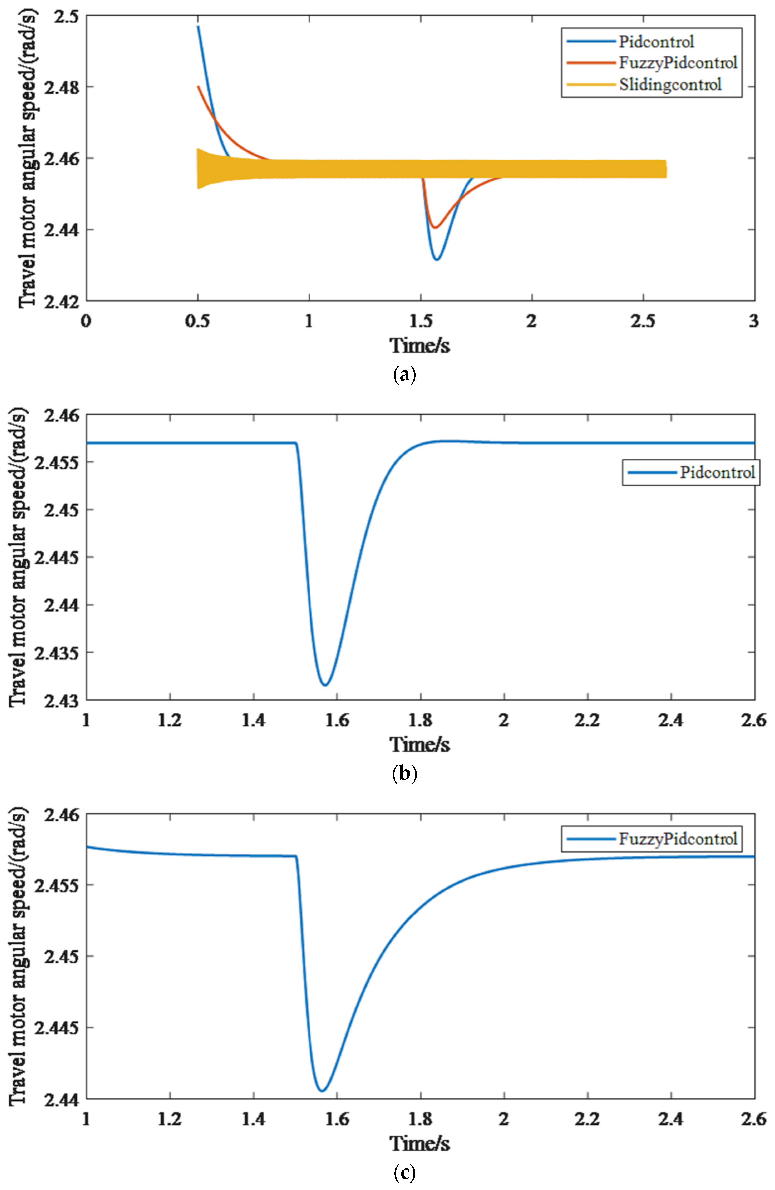
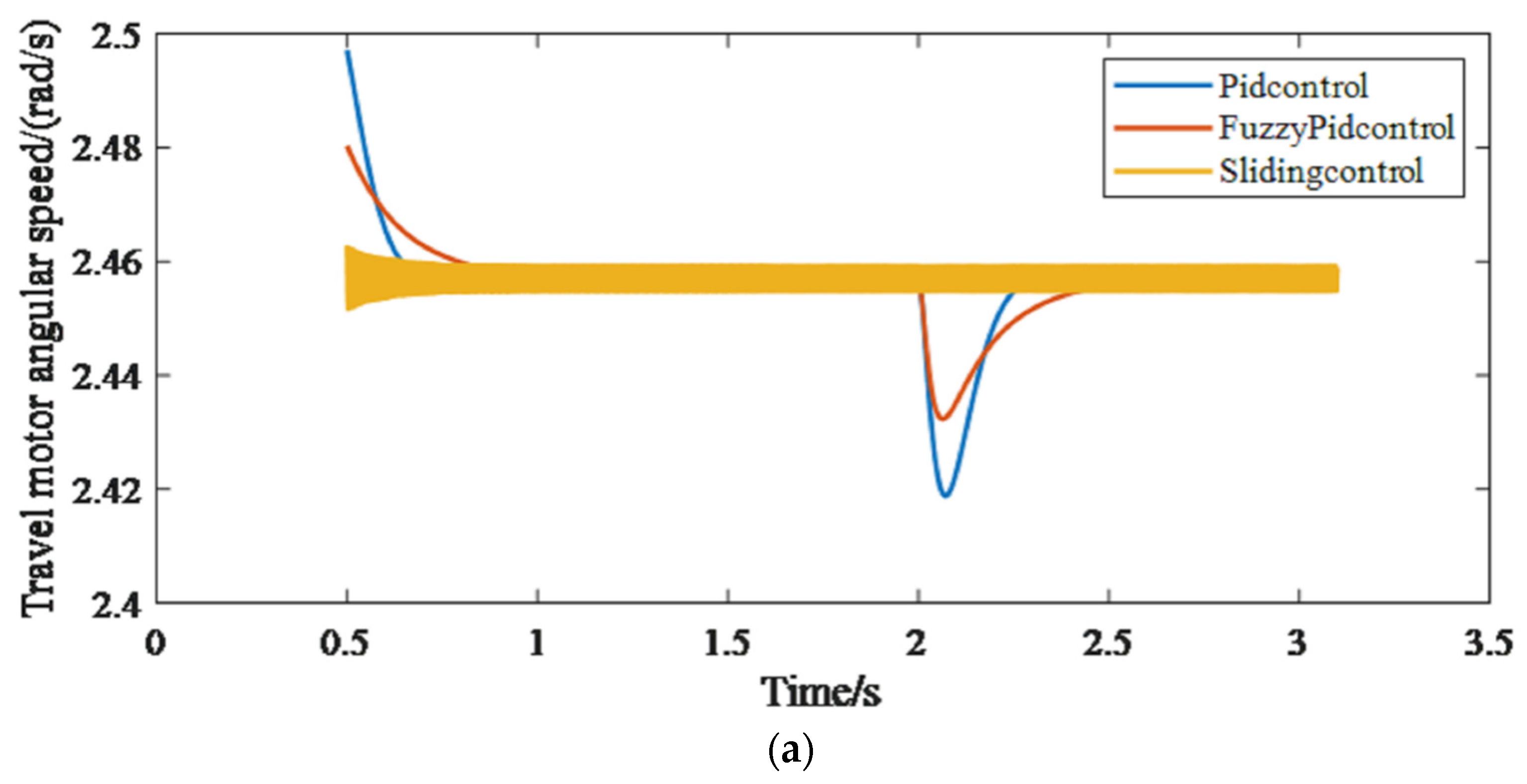
3.1. Results of the Simulation Tests
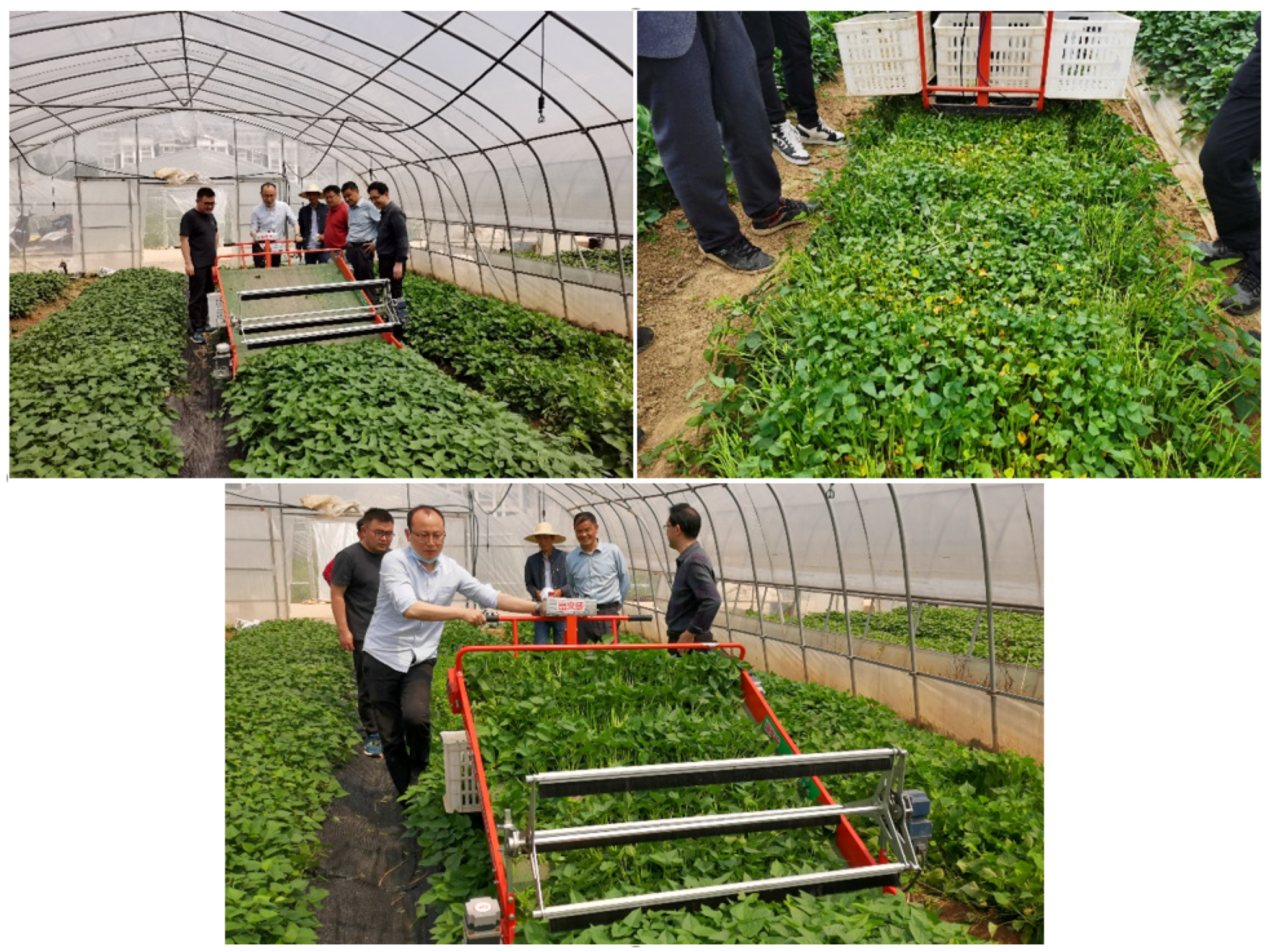
3.2. Results of Field Trials
4. Conclusions
Author Contributions
Funding
Data Availability Statement
Conflicts of Interest
References
- Wang, J.; Du, D.; Hu, J.; Zhu, J. Vegetable Mechanized Harvesting Technology and Its Development. Trans. Chin. Soc. Agric. Mach. 2014, 45, 81–87. [Google Scholar]
- Shen, G.; Wang, G.; Hu, L.; Yuan, J.; Wang, Y.; Wu, T.; Chen, X. Development of harvesting mechanism for stem tips of sweet potatoes. Trans. Chin. Soc. Agric. Eng. 2019, 35, 46–55. [Google Scholar]
- Liu, Z.; Zhang, Z.; Luo, X.; Wang, H.; Huang, P.; Zhang, J. Design of automatic navigation operation system for Lovol ZP9500 high clearance boom sprayer based on GNSS. Trans. Chin. Soc. Agric. Eng. 2018, 34, 15–21. [Google Scholar]
- Hu, J.; Gao, L.; Bai, X.; Li, T.; Liu, X. Review of research on automatic guidance of agricultural vehicles. Trans. Chin. Soc. Agric. Eng. 2015, 31, 1–10. [Google Scholar]
- Ji, C.; Zhou, J. Current situation of navigation technologies for agricultural machinery. Trans. Chin. Soc. Agric. Mach. 2014, 45, 44–54. [Google Scholar]
- Xie, B.; Wu, Z.; Mao, E. Development and prospect of key technologies on agricultural tractor. Trans. Chin. Soc. Agric. Mach. 2018, 49, 1–17. [Google Scholar]
- He, J.; Zhu, J.; Zhang, Z.; Luo, X.; Gao, Y.; Hu, L. Design and experiment of automatic operation system for rice transplanter. Trans. Chin. Soc. Agric. Mach. 2019, 50, 17–24. [Google Scholar]
- Zhao, L.; Zhang, Z.; Wang, C.; Jian, S.; Liu, T.; Cui, D.; Ding, X. Design of integrated monitoring system for wheat precision seeding and fertilization based on variable distance photoelectric sensor. Trans. Chin. Soc. Agric. Eng. 2018, 34, 27–34. [Google Scholar]
- An, X.; Fu, X.; Meng, Z. Construction and verification of photoelectric signal and harvester grain yield data conversion model. Trans. Chin. Soc. Agric. Eng. 2017, 33 (Suppl. S1), 36–41. [Google Scholar]
- Wang, Z.; Pei, J.; He, J. Development of rice precision hole direct seeding machine sowing monitoring system. Trans. Chin. Soc. Agric. Eng. 2020, 36, 9–16. [Google Scholar]
- Lu, C.; Fu, W.; Zhao, C.; Mei, H.; Meng, Z.; Dong, J.; Gao, N.; Wang, X.; Li, L. Design and experiment of real-time monitoring system for wheat sowing. Trans. Chin. Soc. Agric. Eng. 2017, 33, 32–40. [Google Scholar]
- Sun, D.; Qin, D.; Wang, Y. Study on fuzzy control strategy of CVT system for automatic vehicles. Trans. Chin. Soc. Agric. Mach. 2001, 3, 7–10. [Google Scholar]
- Li, X.; Zhang, J.; Yun, Y. Design and Experiment on an Intelligent Control System for Small Electric Leafy Vegetable Harvester. J. Agric. Mech. Res. 2020, 42, 83–87. [Google Scholar]
- Miao, P. Research on Intelligent Control System of Electric Leaf Vegetable Harvester. Master’s Thesis, Jiangsu University, Zhenjiang, China, 2020. [Google Scholar]
- Guo, H.; Gao, G.; Zhou, W.; Lu, Q.; Hao, L. Design and Test of Automatic Control System for Walking Speed of Wheeled Self-propelled Square Baler. Trans. Chin. Soc. Agric. Mach. 2019, 50, 107–114. [Google Scholar]
- Jia, H.; Lu, Y.; Qi, J. Photoelectric sensors combined with rotary encoders to detect the suction performance of suction metering devices. Trans. Chin. Soc. Agric. Eng. 2018, 34, 28–39. [Google Scholar]
- Guo, N.; Hu, J. Variable universe adaptive Fuzzy-PID control of traveling speed for rice transplanter. Trans. Chin. Soc. Agric. Mach. 2013, 44, 245–251. [Google Scholar]
- Zhang, Y.; Li, Y.; Liu, X.; Tao, J.; Liu, C.; Li, R. Fuzzy adaptive control method for autonomous rice seeder. Trans. Chin. Soc. Agric. Mach. 2018, 49, 30–37. [Google Scholar]
- Wang, H.; Zhou, B.; Fang, S. A PMSM Sliding Mode Control System Based on Exponential Reaching Law. Trans. China Electrotech. Soc. 2009, 24, 71–77. [Google Scholar]
- Li, J.; Shang, Z.; Li, R.; Cui, B. Adaptive Sliding Mode Path Tracking Control of Unmanned Rice Transplanter. Agriculture 2022, 12, 1225. [Google Scholar] [CrossRef]
- Chen, J.; Zhang, H.; Pan, F.; Du, M.; Ji, C. Control System of a Motor-Driven Precision No-Tillage Maize Planter Based on the CANopen Protocol. Agriculture 2022, 12, 932. [Google Scholar] [CrossRef]
- Bai, S.; Yuan, Y.; Niu, K.; Shi, Z.; Zhou, L.; Zhao, B.; Wei, L.; Liu, L.; Zheng, Y.; An, S.; et al. Design and Experiment of a Sowing Quality Monitoring System of Cotton Precision Hill-Drop Planters. Agriculture 2022, 12, 1117. [Google Scholar] [CrossRef]
- Zhang, B.; Chen, X.; Zhang, H.; Shen, C.; Fu, W. Design and Performance Test of a Jujube Pruning Manipulator. Agriculture 2022, 12, 552. [Google Scholar] [CrossRef]
- Tian, F.; Wang, X.; Yu, S.; Wang, R.; Song, Z.; Yan, Y.; Li, F.; Wang, Z.; Yu, Z. Research on Navigation Path Extraction and Obstacle Avoidance Strategy for Pusher Robot in Dairy Farm. Agriculture 2022, 12, 1008. [Google Scholar] [CrossRef]


| Parameters | Values |
|---|---|
| Whole machine size (length × width × height)/(mm × mm × mm) | 2180 × 1500 × 1200 |
| Battery capacity/ | 50 |
| Working width/ | 1200 |
| Cutter height adjustment range/ | 0~100 |
| Conveyor belt width/ | 1200 |
| Conveyor belt installation inclination/ | 30 |
| Wheel base/ | 550 |
| Wheel radius/ | 175 |
| Minimum ground clearance/ | 70 |
| Productivity/ | 0.04–0.08 |
| e | ec | ||||||
|---|---|---|---|---|---|---|---|
| NB | NM | NS | ZO | PS | PM | PB | |
| NB | PB | PB | PM | PM | PS | PS | ZO |
| NM | PB | PB | PM | PM | PS | ZO | ZO |
| NS | PM | PM | PM | PS | ZO | NS | NM |
| ZO | PM | PS | NS | ZO | NS | NM | NM |
| PS | PS | PS | ZO | NS | NS | NM | NM |
| PM | ZO | ZO | NS | NM | NM | NM | NB |
| PB | ZO | NS | NS | NM | NM | NB | NB |
| e | ec | ||||||
|---|---|---|---|---|---|---|---|
| NB | NM | NS | ZO | PS | PM | PB | |
| NB | NB | NB | NB | NM | NM | ZO | ZO |
| NM | NB | NB | NM | NM | NS | ZO | ZO |
| NS | NM | NM | NS | NS | ZO | PS | PS |
| ZO | NM | NS | NS | ZO | PS | PS | PM |
| PS | NS | NS | ZO | PS | PS | PM | PM |
| PM | ZO | ZO | PS | PM | PM | PB | PB |
| PB | ZO | ZO | PS | PM | PM | PB | PB |
| Working Condition Numbers | Names | Specific Situations |
|---|---|---|
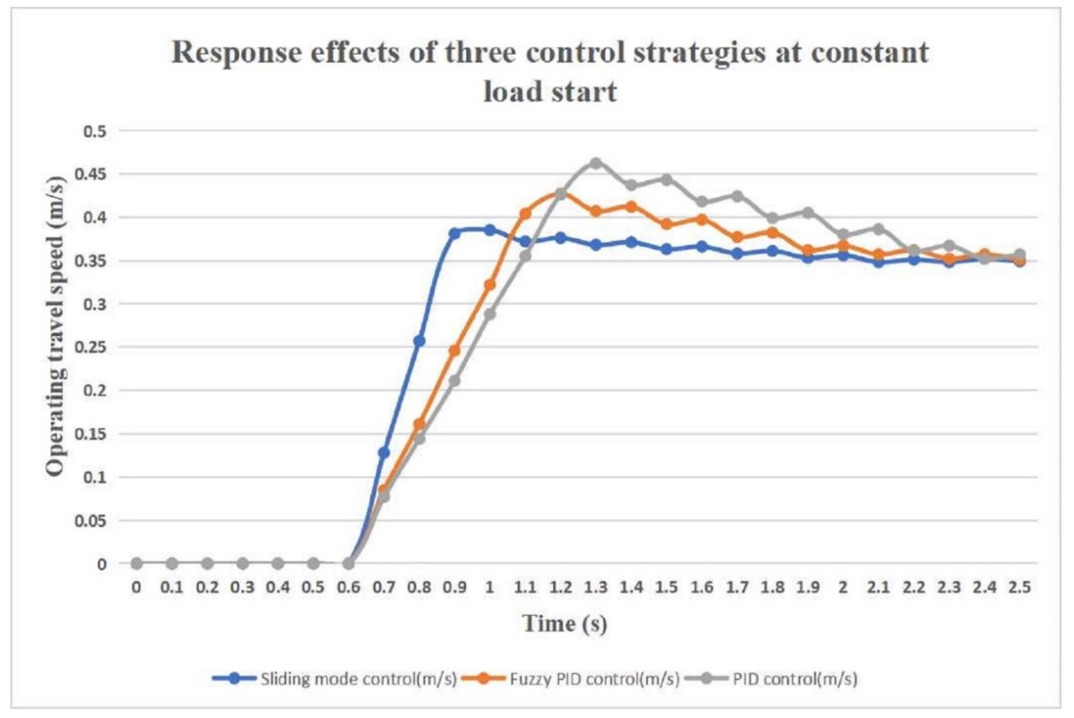
| Working condition 1 | Constant load starting of travel motor | Constant, unvarying load during start-up of the travel motor |
| Working condition 2 | Sudden increase in load when the travel motor was running smoothly | Harvester climbing suddenly in smooth running operation |
| Working condition 3 | Sudden increase in load when the travel motor was running smoothly | Harvester crossing bump suddenly in smooth running condition |
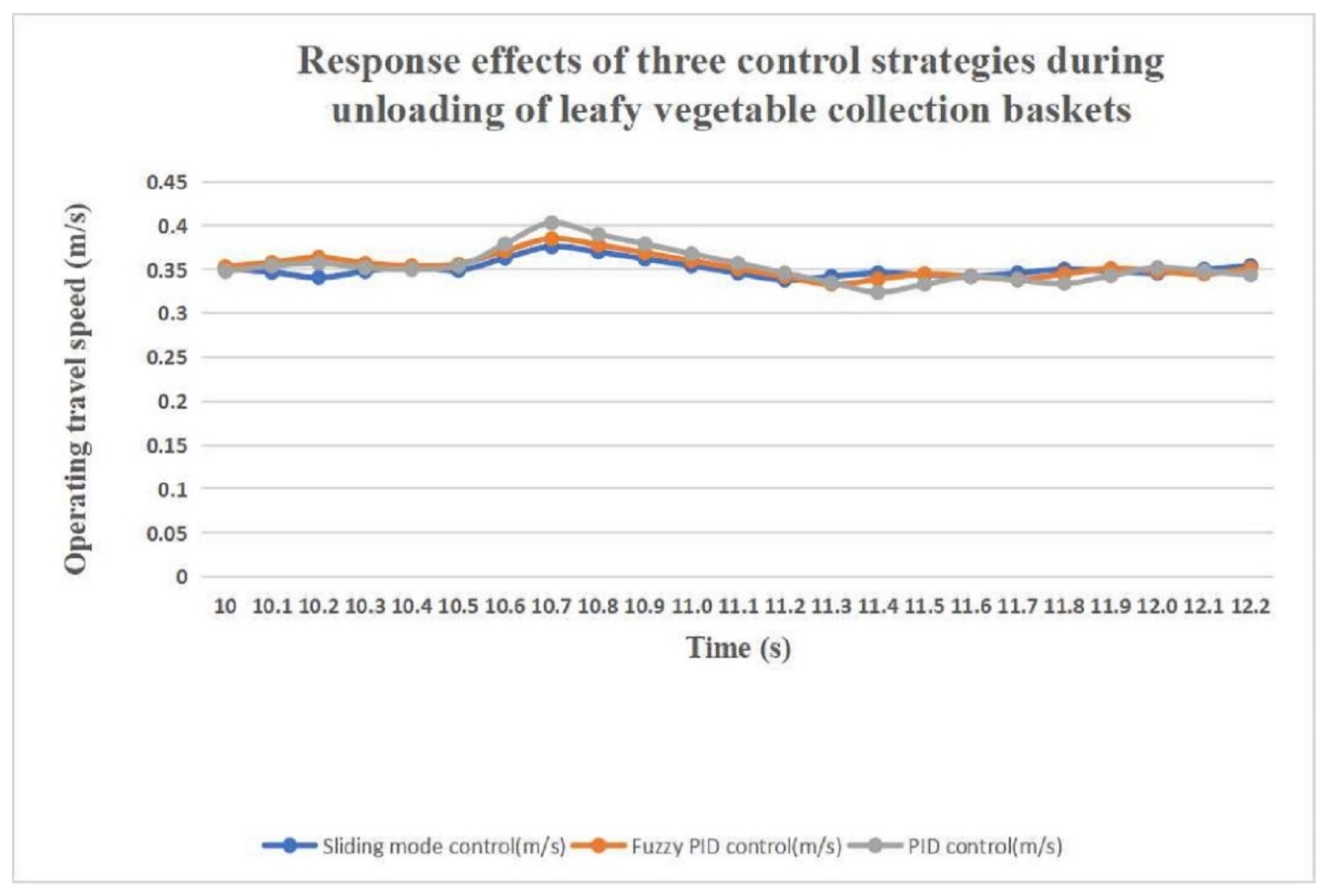
| Working condition 4 | Sudden decrease in load when the travel motor was running smoothly | Harvester in smooth running condition with leafy vegetable collection baskets filled and unloaded |
Publisher’s Note: MDPI stays neutral with regard to jurisdictional claims in published maps and institutional affiliations. |
© 2022 by the authors. Licensee MDPI, Basel, Switzerland. This article is an open access article distributed under the terms and conditions of the Creative Commons Attribution (CC BY) license (https://creativecommons.org/licenses/by/4.0/).
Share and Cite
Chen, W.; Wang, G.; Hu, L.; Yuan, J.; Wu, W.; Bao, G.; Yin, Z. Research on the Control Strategy of Leafy Vegetable Harvester Travel Speed Automatic Control System. AgriEngineering 2022, 4, 801-825. https://0-doi-org.brum.beds.ac.uk/10.3390/agriengineering4040052
Chen W, Wang G, Hu L, Yuan J, Wu W, Bao G, Yin Z. Research on the Control Strategy of Leafy Vegetable Harvester Travel Speed Automatic Control System. AgriEngineering. 2022; 4(4):801-825. https://0-doi-org.brum.beds.ac.uk/10.3390/agriengineering4040052
Chicago/Turabian StyleChen, Wenming, Gongpu Wang, Lianglong Hu, Jianning Yuan, Wen Wu, Guocheng Bao, and Zicheng Yin. 2022. "Research on the Control Strategy of Leafy Vegetable Harvester Travel Speed Automatic Control System" AgriEngineering 4, no. 4: 801-825. https://0-doi-org.brum.beds.ac.uk/10.3390/agriengineering4040052