Modelling Hydrological Processes in Agricultural Areas with Complex Topography


1
Institute of BioEconomy-CNR, Via Madonna del Piano 10, Sesto Fiorentino, 50019 Florence, Italy
2
Department of Agriculture, Food, Environment and Forestry (DAGRI)—University of Florence, Piazzale delle Cascine, 18-50144 Florence, Italy
*
Author to whom correspondence should be addressed.
Agronomy 2020, 10(5), 750; https://0-doi-org.brum.beds.ac.uk/10.3390/agronomy10050750
Submission received: 25 April 2020
/
Revised: 19 May 2020
/
Accepted: 21 May 2020
/
Published: 22 May 2020
Abstract
:Agricultural intensification and soil mismanagement have been recognized among the main causes of soil erosion in Mediterranean climate areas such as the Arbia stream basin (Tuscany, Italy). This study aims at predicting soil loss from agricultural fields as it is essential for providing reliable information for prioritizing soil conservation measures. Thus, measured soil loss from 243 agricultural fields within the Arbia stream basin during the period 2007–2010 were used to calibrate and validate the ArcSWAT 2012 model at hydrological response units (HRU) scale. Analysis of variance with post-hoc Tukey honest significant test was used to assess significant measured soil loss differences between slope steepness classes and land covers. Soil loss estimation was always “very good” for irrigated field crops, olive groves, and vineyards, “good” for unirrigated field crops, and “unsatisfactory” for broad-leaved forest. The model succeeded in the quantitative assessment of erosive processes at HRU scales. Its application to the whole Arbia stream basin estimated that 31% of the total surface is subjected to higher erosion levels. This approach might help facilitate the identification of priority areas that need the implementation of conservation measures.
1. Introduction
Agricultural intensification, soil mismanagement, and heavy rains following dry periods have been recognized among the predominant causes of soil erosion exacerbation in areas characterized by Mediterranean climate [1,2,3]. The Arbia stream basin (Tuscany, Italy), which lies within the “Crete Senesi” area [4,5], is a representative example reflecting this situation.
As soil is considered a limited resource that requires a long time to be recovered [6], effective sustainable soil management is extremely important. Several studies have investigated the risk of soil erosion on different spatial levels [1,7] with the objective of providing scientific support for decision-makers to adopt correct land-management measures. An essential condition to support land management is the availability of a simulation model that can reliably simulate hydrological dynamics at various scales because field monitoring is demanding in terms of costs and human resources [7,8]. This gap can be addressed by using models to analyze the effect of land use/cover, pedo-morphology, and climate on hydrological processes.
The Soil and Water Assessment Tool (SWAT) [9] is a model used worldwide to estimate flow dynamics and soil erosion of basins with dimensions varying from hectares to regional scale [10]. This model can be used to simulate a large variety of hydrologic processes such as water runoff and soil loss at several geographical scales. Nevertheless, the SWAT model can be reliably applied to the evaluation of the impact of agricultural practices provided that model parameterization is determined and validated by field studies [11]. Indeed, there are very few published works dedicated to the validation of soil loss estimates, because such a validation is very challenging [12]. For this reason, the reliability of a simulation model in estimating soil loss simulation is commonly assessed by a validation that is performed at the outlet of the basin [13]. Nevertheless, the so-called outlet-based validation can result in an underestimation of soil loss, because deposition can occur along the path towards the catchment outlets [14,15]. Therefore, model performance evaluation at the field scale level is needed.
This study aims to evaluate the effectiveness of ArcSWAT2012 in estimating soil loss from agricultural fields in basins with complex topography and different land use and its potential application in providing reliable information for prioritizing soil conservation measures. The model was tested in the Arbia stream basin to estimate both water runoff and soil loss from agricultural fields. Model validation was assessed by comparing daily estimated and measured runoff at the gauging station and by comparing estimated and measured annual soil losses from 243 agricultural fields within the Arbia stream basin. Finally, the validated model was used to produce erosion risk maps of the study area.
2. Materials and Methods
2.1. Characteristics of the Arbia Stream Basin
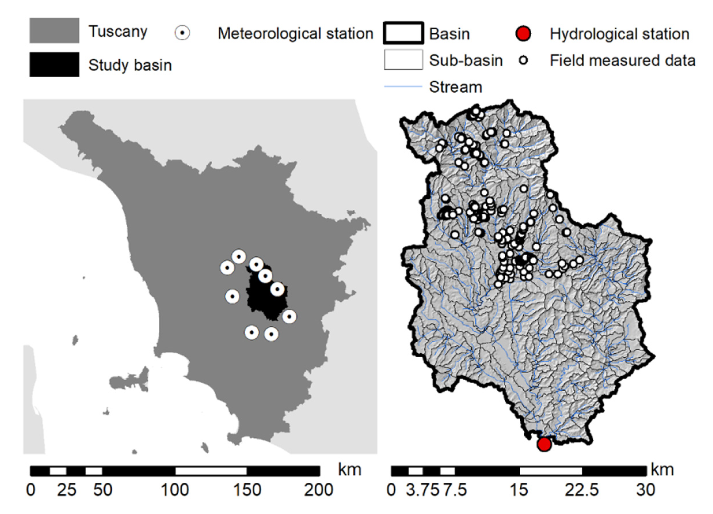
The Arbia stream basin is located in central Tuscany (Italy) between latitudes 43.13° and 43.50° North and between longitudes 11.27° and 11.65° East (Figure 1). The basin has an area of 765 km2 with elevations ranging between 134 and 780 m a.s.l., at the gauging station and at the highest part of the basin, respectively. The Arbia stream flows in a north to southerly direction for about 57 km and with an average stream flow of approximately 3.5 m3s−1. The climate is Mediterranean with m annual rainfall of about 750 mm, a maximum of 93 mm in October and a minimum of 31 mm in July. Similar to other areas in central Tuscany, rainfall mainly occurs in autumn and spring [16,17]. July is the hottest month (22 °C) and January the coldest (5 °C).
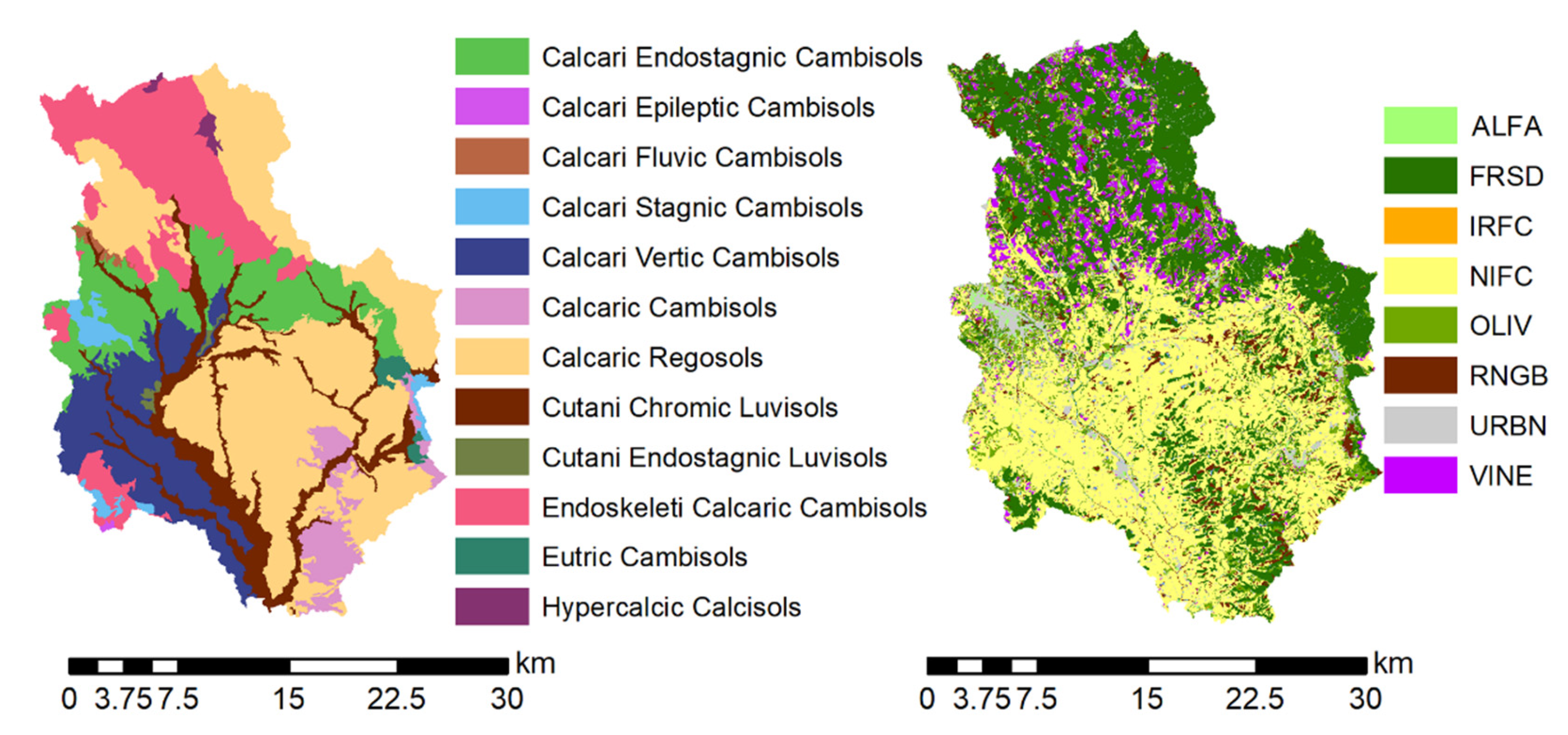
The soil map of Tuscany [18] was used to identify the soil characteristics in the Arbia stream basin (Figure 2). Clay loam soils, originating from both the Eocene calcareous marl (Endoskeleti Calcaric Cambisols and Calcaric Regosols) [19] and from layers of clays intercalated by gypsum lens (Hypercalcic Calcisols), predominate the northern part of the basin. Silty clay loam soils, generated from clay schist and marly limestone (Calcari Endostagnic Cambisols), exist as a transversal band in the center of the basin. Pliocene-derived sandy soils are mainly located in the west (Calcari Stagnic Cambisols). Pliocene-derived clay soils dominate the south-western (Calcari Vertic Cambisols) and the south-eastern parts (Calcic Regosols and Calcaric Cambisols) of the basin. Finally, silty clay soil, originating from travertine rock (Cutani Chromic Luvisols) is found on the Arbia stream valley floor.
2.2. Characteristics of the Arbia Stream Basin
The study was performed over a period starting from June 2006 to December 2010. Daily meteorological and streamflow data were obtained by the Regional Hydrological Service [20]. Daily rainfall height (P; mm) and maximum and minimum air temperature (Tmax and Tmin; °C) of nine available weather stations within the basin were used for this study. Streamflow data were obtained from the flow station near Buonconvento (Figure 1). Linear interpolation with data of the nearest available station was performed to estimate missing meteorological data [21].
The 1:250,000 soil map from the regional geodatabase [18] was used to derive the soil parameters. Then, the soils within the basin were classified into Hydrologic Soil Groups (HSG), from A to D according to their runoff potential [22].
The 10 m pixel Digital Elevation Model (DEM) and the land cover map, dating from 2012, were provided by the Tuscany Region cartographic service [23]. Eight principle categories of land cover classes were defined as follows: artificial surfaces (URBN); broad-leaved forest (FRSD); transitional woodland-shrub-brush (RNGB); meadow (ALFA); irrigated field crops (where sunflower, maize, and grain sorghum cultivation comprised more than the 90% of the surface area) (IRFC); unirrigated field crops (where winter wheat, winter barley, and oat cultivation constituted more than the 60% of the surface area) (NIFC); olive groves (OLIV); and vineyards (VINE).
Soil loss data measured by [2] from 243 fields within the study area, from the year 2007 to 2010, were used to validate the SWAT model. Each field was characterized by having homogeneous slope, land cover, and soil type, and by having an area ranging from 0.2 to 14.9 ha (average 4.9 ha). Soil loss data were grouped for comparison with the defined vegetation and crops classes (Table 1).
2.3. The ArcSWAT Set-Up
ArcSWAT 2012 extension for ArcGIS 10.3 [24] was used for modelling water flow and soil losses. ArcSWAT delineated streams, basin, and sub-basins based on the DEM. The model generated a total of 397 sub-basins, characterized by an average surface area of about 192.6 ha. ArcSWAT divided each basin into hydrological response units (HRU) [25]. Five slope classes were considered for defining HRU, as follows: 0%–3%, 3%–10%, 10%–20%, 20%–30%, and >30%.
A total of 22,634 HRU were delineated within the Arbia stream basin, with an area ranging from 0.1 to 267.7 ha (average 3.4 ha).
The model routed the runoff flows generated by each HRU through the channel network, thereby simulating the basin. The model generated the total flow (Qt; mm) in the channel network by summing the surface flow (Qs; mm), lateral flow (Ql; mm), and base flow (Qb; mm). Both Ql and Qb were computed as suggested in Sloan and Moore [26] and Neitsch et al. [9], respectively. Qs was modelled using the Curve Number (CN) method [27] as reported in [21]. The CN accounts for several factors affecting the surface flow generation such as soil characteristics, land cover and land use practices, vegetative season, and antecedent moisture condition (AMC) [28] (Table 2).
The SWATsoil database was integrated with parameters related to each soil unit of the basin, such as number of horizons, horizon depth, soil texture, gravel percentage, bulk density, porosity, saturated hydraulic conductivity, hydrological soil group, available water capacity, organic carbon percentage, electrical conductivity, and soil erodibility factor (K factor) [9]. The K factor was calculated according to Wischmeier et al. [30].
SWAT accounted for ground cover impact on soil loss by means of the USLE cover and management factor (C factor). This latter factor was updated daily as function of the amount of soil cover and the lower threshold of C factor (USLE_C; Table 3) defined for each land cover [9]. For all land covers, USLE_C values were set as reported in Napoli et al. [2].
2.4. Model Evaluation and Statistical Analysis
As suggested by Di Luzio et al. [32], a “warm up” period of 1 year was used to account for model difficulty in predicting the soil hydrology caused by the initial conditions. In this study, “warm up” was performed from June 2006 to December 2006. Then, the simulation continued from January 2007 to until December 2010, and only the results within this period were used for the analysis.
The model performance was measured and analyzed by adopting the statistical criteria and score classification proposed by Moriasi et al. [33], using the percentage bias (PBIAS), the ratio of the root mean square error to observation standard deviation (RSR), and the Nash–Sutcliffe coefficient (NSC) [34]. In particular, according to Moriasi et al. [33] a PBIAS value lower than 10%, between 10%–15% and 15%–25%, and over 25% was considered “very good”, “good”, “satisfactory”, and “unsatisfactory”, respectively. Moreover, a RSR was considered “very good”, “good”, “satisfactory”, and “unsatisfactory” when values were lower than 0.5, between 0.5–0.6 and 0.6–0.7, and over 0.7, respectively. Further, a NSE was considered “very good”, “good”, “satisfactory”, and “unsatisfactory” when values were higher than 0.75, between 0.75–0.65, 0.65–0.5, and less than 0.5, respectively.
Model performance in predicting flow was performed by analyzing the daily difference between estimated and actual flow of the basin outlet over the study period. The soil loss predictability was assessed by comparing the yearly on-field measured soil loss data with the modeled one from the corresponding HRU.
Statistical indices were calculated both on the whole period and on an annual and seasonal basis. The analysis of variance (ANOVA) was used to test for significant differences (p < 0.05) of measured soil loss between steepness classes for each land cover. Post-hoc analysis was performed by means of the Tukey honest significance test (Tukey-HSD), using a significance level of p < 0.05.
3. Results
3.1. Model Evaluation and Statistical Analysis
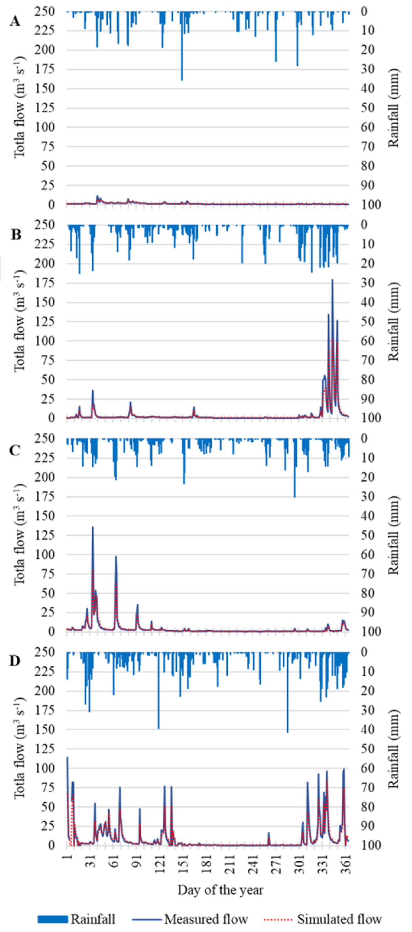
Daily total flow calculated by the model had a good fit on actual flow (Figure 3). Results indicated that the model overestimated total flow under dry conditions and underestimated total flow under high rainfall conditions, respectively.
However, according to the adopted statistical indicators, ArcSWAT scored a “very good” performance when simulating the daily total flow over the considered period (Table 4). Model performance, in estimating annual and seasonal total flow, was always “very good” except for 2007 (PBIAS = −14.3%) and the summer periods of each year (PBIAS = −19.8%). Nonetheless, in both the latter cases, the performance was still considered “good”.
3.2. Measured Soil Loss Differences between Steepness Classes
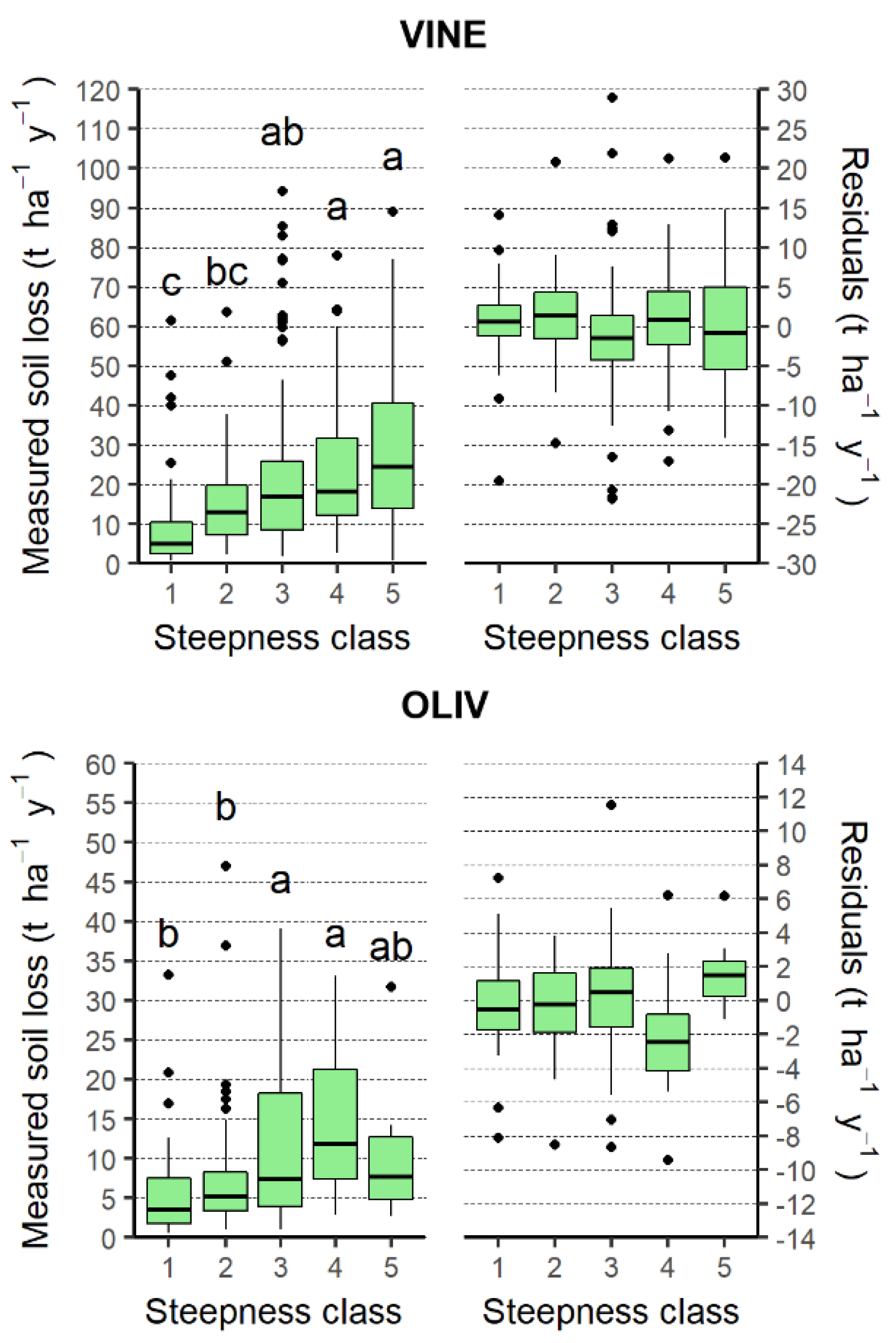
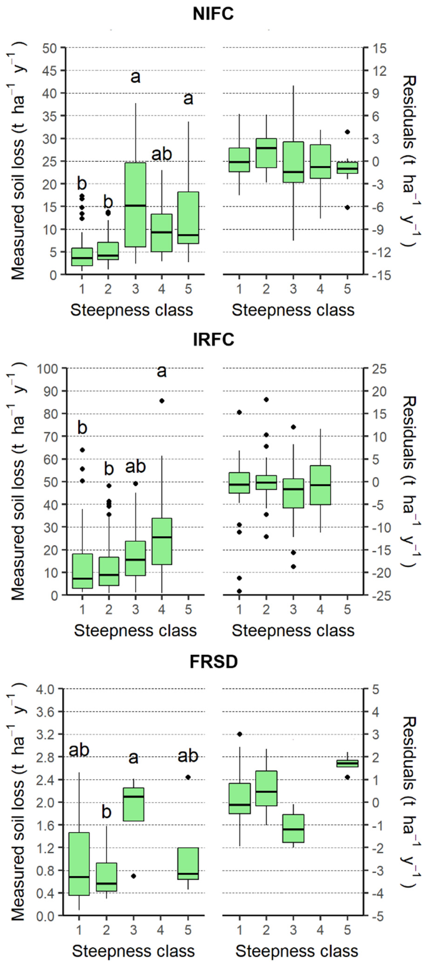
VINE (20.2 t·ha−1·y−1) scored the highest average soil loss, followed by IRFC (16.92 t·ha−1·y−1), OLIV (8.62 t·ha−1·y−1), and NIFC (8.41 t·ha−1·y−1), while FRSD (0.93 t·ha−1·y−1) scored the lowest one (Figure 4 and Figure 5).
Steepness affected soil loss differently depending on the type of land cover (Figure 4 and Figure 5). VINE was characterized by increasing soil loss while steepness increased, with significant differences in averaged values: between the 1st steepness slope class (10 t·ha−1·y−1) and 3rd, 4th, and 5th (respectively, 21.4, 23.6, and 29 t·ha−1·y−1), between 2nd steepness slope class (15.3 t·ha−1·y−1) and 4th and 5th steepness classes (23.6 and 29 t·ha−1·y−1) (Figure 4).
Finally, only a significant difference between the 2nd (0.71 t·ha−1·y−1) and 3rd (1.83 t·ha−1·y−1) steepness class was found for FRSD.
Even for OLIV, the effect of soil erosion increased with steepness class, except for the 5th class (Figure 4). Soil loss for the 1st and 2nd classes (respectively, 5.56 and 7.3 t·ha−1·y−1) was significantly lower than the 3rd and 4th classes (respectively, 11.76 and 14.17 t·ha−1·y−1) (Figure 4). IRFC presented a similar pattern to OLIV. Indeed, the first two steepness classes (respectively, 2.62 and 12.66 t·ha−1·y−1) were significantly lower than the 4th steepness class (25.62 t·ha−1·y−1) and the 3rd (18.54 t·ha−1·y−1) was not significantly different from any of the previous ones (Figure 5). None of the measured fields fell in the 5th steepness class.
For NIFC, the 1st and 2nd steepness classes (respectively, 4.81 and 5.58 t·ha−1·y−1) were significantly different from the 3rd and 5th classes (respectively, 15.7 and 12.97 t·ha−1·y−1), while 4th steepness class (9.97 t·ha−1·y−1) was not significantly different from all the classes (Figure 5).
3.3. Validation of Soil Loss Estimates
The model applied to VINE fields overestimated average soil loss for all the steepness classes (0.59, 1.38, 0.91, and 0.22 t·ha−1·y−1 for the 1st, 2nd, 4th, and 5th, respectively) except the 3rd that was underestimated by 1.5 t·ha−1·y−1. Performance on VINE was considered “very good” for the 2nd to the 5th, steepness classes, while resulting unsatisfactory for the 1st steepness class (Table 5).
Soil loss simulations on OLIV were considered “very good” regardless of the steepness class (Table 5), though 1st, 2nd, and 4th steepness classes were overestimated (0.33, 0.36, and 2.08 t·ha−1·y−1, respectively) and the 3rd and 5th steepness classes were underestimated (0.12 and 1.68 t·ha−1·y−1, respectively).
Additionally, for IRFC, model performance was very good for any class. Estimated values for the 1st and 3rd were higher than measured ones, respectively, by 0.98 and 2.65 t·ha−1·y−1, and for the 2st and 4th were lower than the measured ones by 0.02 and 0.65 t·ha−1·y−1, respectively.
For NIFC, the two lower steepness classes (0.28 and 1.17 t·ha−1·y−1) were overestimated, while the other ones were underestimated for the remaining classes (1.06, 0.64, and 1.01 t·ha−1·y−1). ArcSWAT obtained the worst performance on NIFC, because skill indices were “very good” only for the 5th class, “good” for 1st, 3rd, and 4th. Performance for the 2nd class was “unsatisfactory” and the reason for that could be probably ascribable to the limited number of available data on that class.
ArcSWAT performance always resulted in “unsatisfactory” for FRSD. Here soil losses were overestimated by about 0.11, 0.59, and 1.68 t·ha−1·y−1, for the 1st, 2nd, and 5th steepness classes, respectively, and underestimated by about 1.12 for the 3rd steepness class.
3.4. Estimation of the Soil Loss within the Basin
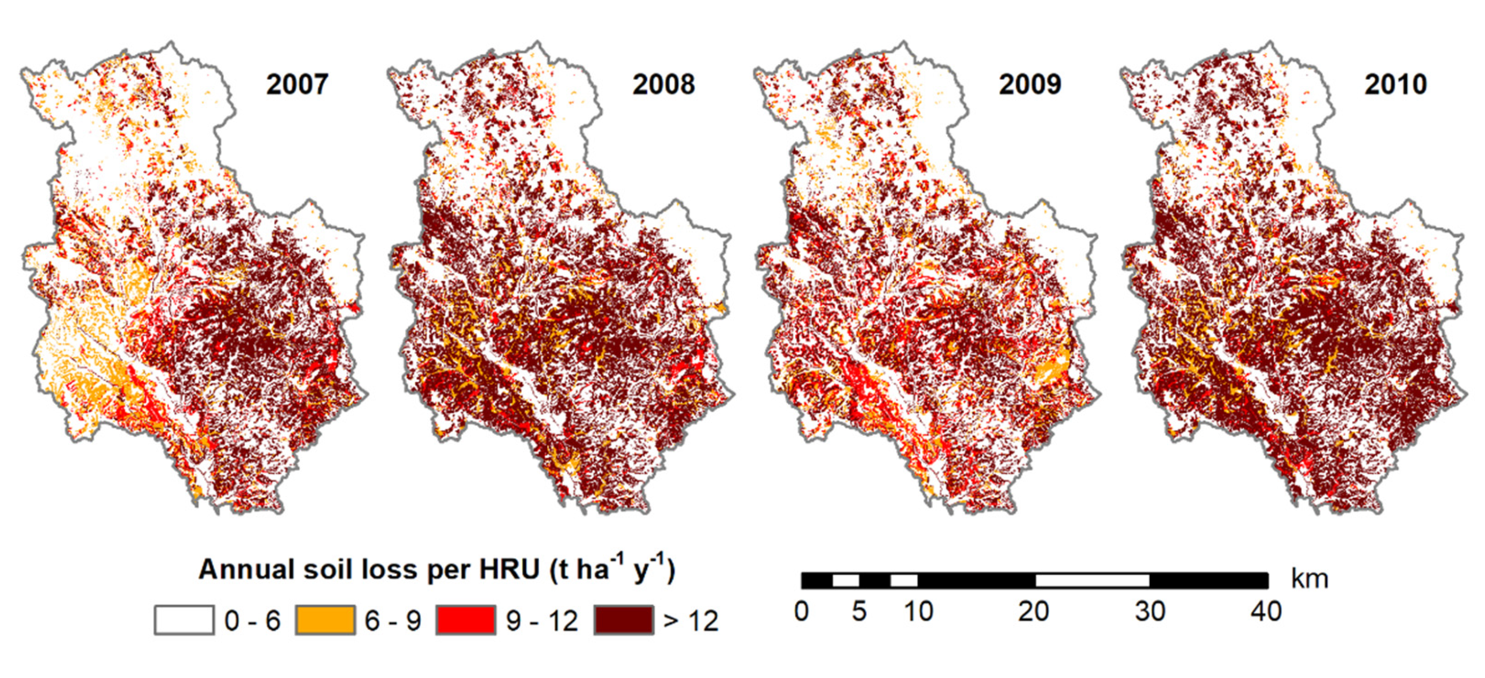
Figure 6 shows the simulated soil losses (HRU level) in the Arbia stream basin for each year under analysis. The estimated average annual soil loss varied between 6.89 and 11.85 t·ha−1·y−1 in the studied period. These values were higher than 6 t·ha−1·y−1 that is the tolerable soil loss limit set by OECD [35]. During the study period, 14.5%, of the basin area was moderately affected by erosion (6–12 t·ha−1·y−1), with an inter-annual variation ranging between 9% and 19.8%.
In turn, approximately 31% of the basin surface area showed a higher erosion level (>12 t·ha−1·y−1), with an inter-annual variation 22.4% and 41.2%. Within the basin, the areas that were subjected to the most frequent occurrence of intense soil losses included the following: soils that were a combination of Calcaric Cambisols and Calcari Endostagnic Cambisols, moderate to very steep slopes (comprising steepness classes 3, 4, and 5), land cover coverage with VINE, OLIV, and NIFC.
The model indicated that VINE produced the highest soil loss values, both in terms of average and maximum soil losses per year (Table 6).
On average, during the study period, the predicted average annual soil losses in VINE were 2.05 times (ranging between 1.22 and 3.04 times) higher than the tolerable limit set by OECD [35]. Even, predicted soil loss in IRFC (15.48 t·ha−1·y−1 on average) and OLIV (10.09 t·ha−1·y−1 on average) were higher than the tolerable limit during the entire study period. On average, the estimated annual soil losses for NIFC were moderate (8.99 t·ha−1·y−1 on average), exceeding the tolerable limit for 3 out of 4 years. Over the entire basin, the model estimated tolerable average annual soil losses for FRSD (1.42 t·ha−1·y−1 in average). The simulation results also suggested that the estimated maximum annual values for FRSD could be higher than the tolerable limit in areas with slope values exceeding 20%. During the study period, both the average and maximum annual soil losses estimated for the RNGB and ALFA land covers were lower than the tolerable soil loss limit.
These estimates can be considered reliable because the model was validated on land covers that represent 90% of the whole river basin area and 5% of the remaining area was artificial surfaces that does not contribute to soil loss.
4. Discussion
4.1. Water Flow
Although the model analysis was conducted using the settings that were calibrated for the nearby basin of the Elsa stream [21], all statistical indices scored a “good” to “very good” performance, thus indicating no model overfitting. Statistical indices and hydrographs highlighted that model performance resulted in “very good” when high flow occurs, such as during the years 2008, 2009, and 2010. Conversely, the model was shown to be less accurate during low flow periods such as in the year 2007. As previously observed, the model overestimated flow during dry periods [21]. Gebremariam et al. [36] also reported the difficulty of SWAT in modeling flow under dry conditions. Moreover, as previously observed [37], the model showed difficulty in simulating total flow when intense or prolonged rainfall occurred. Regardless of the difficulty in simulating total flow, both under dry conditions and high or prolonged rainfall, the statistical criteria indicated that model performance ranged between “good and very good”. In general, model performance resulted in “very good” within the Arbia stream basin. The overestimation of daily total flow (PBIAS always negative) can be considered a conservative evaluation of the risk.
4.2. Soil Loss
Our simulation results on VINE are in good agreement with values presented by Wicherek [38] and Napoli et al. [21] 35 t·ha−1·y−1 in the mid-Aisne region (France) and 42.1 t·ha−1·y−1 in the Tuscany region (Italy), respectively. The annual maximum predicted values within the basin were consistent with measured soil loss of 102.2 t·ha−1·y−1 reported by Novara et al. [39] in Sicilian vineyards (Italy) with conventionally tilled inter-rows. The average soil loss measured in OLIV was higher than that measured by Gómez et al. [40] and Napoli and Orlandini [41] in olive orchards with either grass or mulch cover. These authors reported average annual soil losses of about 1.2 t·ha−1·y−1 in Cordoba and 3.5 t·ha−1·y−1 in central Italy, respectively. Conversely, higher soil losses (82.8 t·ha−1·y−1) in olive orchards maintained on bare soil were measured in southern Italy by Raglione et al. [42]. The average soil loss values measured for NIFC were higher than that measured by Romero-Dìaz et al. [43] in Spain and that measured by Porqueddu and Roggero [44] in Sardinia (Italy). However, estimated soil erosion was consistent with the measured soil loss data used for validation and was also consistent with the pedo-morphological characteristics of the areas on which NIFC are cultivated locally. NIFC are mainly cultivated within “Crete Senesi” area, where soil erosion has played a major role in the formation of the landscape, with the white and dome-shapes clay knolls that are locally named “biancane”. Estimated soil losses in IRFC were consistent with those measured by Kisić et al. [45] for maize cultivated with ploughing across the slope (11.69 t·ha−1·y−1). On the contrary, Cerdan et al. [46] reported higher soil loss values in erosion plot studies. However, as suggested by Cerdan et al. [46], the limited size of a plot could not effectively represent the sheet and rill erosion processes on a hill-slope scale. Finally, the estimate of average soil losses for FRSD was consistent with the soil loss values measured in the Mediterranean area [46].
These results were subject to various uncertainties which can be considered limitations of the study. Firstly, spatialization of rainfall data in complex terrain areas can result in significant estimation errors [47]. In this context, Tuppad et al. [48] and Martínez-Casasnovas et al. [7] highlighted the variability of responses in ArcSWAT as a function of the rainfall data spatial resolution. Additionally, the time period considered in this study is too limited to take into account the inter-annual precipitation variability and, therefore, to perform a long term soil erosion assessment. Furthermore, the DEM and the soil map used in this work may not be accurate enough to represent the pedo-morphological variability within the Arbia stream basin. Additionally, the parameterization adopted to describe land-use and plant development are not sufficiently reliable in adequately representing the actual fields [49]. Finally, due to the expenses for carrying out field surveys and the difficulty in obtaining permission to site access on private lands, the number and distribution of the fields, in which the erosion was measured, may not be sufficiently adequate for the validation. Regardless of all the above-mentioned uncertainties, the statistical indices indicate that the model achieved very good performance in estimating soil losses at HRU scale. Thus, it can be used for territorial planning and prioritizing soil conservation measures.
5. Conclusions
According to our study, the ArcSWAT model is an effective tool to reproduce hydrological processes in a basin characterized by complex topography and varied land use. Daily runoff at basin scale was estimated accurately by the model using a parameterization that was determined in a previous study performed in the nearby Elsa basin. This result suggests that a model parameterization can be effectively reused for stream basins with similar morphological characteristics and located in a homogeneous geographical area. Soil erosion processes were estimated and validated at field scale, by comparing simulated annual soil losses against measured soil loss, as determined in 243 fields from 2007 to 2010. The model was effective in simulating field soil losses within the study area regardless of the steepness class. Statistical analyses indicated that ArcSWAT provided good or better results in terms of annual soil loss estimates for olive orchard (OLIV), unirrigated field crops (NIFC), and vineyard (VINE). Conversely, some problems were noted in estimating soil losses in both irrigated field crops (IRFC) and deciduous forests (FRSD). Therefore, the erosion maps obtained by ArcSWAT simulations can be considered a reliable picture of soil loss in the Arbia stream basin. According to these maps the ArcSWAT estimated that approximately 45.8% of the surface area of the Arbia stream basin was affected by soil losses that exceed the tolerable set limit (6 t·ha−1·y−1) and about 31.3% of the surface area is affected by high erosion levels (>12 t·ha−1·y−1). These types of maps represent important instruments for the public authorities to plan strategies aiming to the protection and sustainable management of the territory. Moreover, information provided through maps is easy to interpret and facilitate the identification of priority areas of intervention.
Author Contributions
Conceptualization, L.M. and M.N.; methodology, L.M. and M.N.; validation, L.M. and M.N.; formal analysis, L.M. and M.N.; investigation, L.M. and M.N.; funding acquisition, S.O.; data curation, C.G., L.M. and M.N; writing—original draft preparation, C.G., L.M. and M.N; writing—review and editing, L.M. and M.N.; visualization, L.M. and M.N.; supervision, S.O. All authors have read and agreed to the published version of the manuscript.
Funding
This research received no external funding
Conflicts of Interest
The authors declare no conflict of interest.
References
- Panagos, P.; Borrelli, P.; Poesen, J.; Ballabio, C.; Lugato, E.; Meusburger, K.; Montanarella, L.; Alewell, C. The new assessment of soil loss by water erosion in Europe. Environ. Sci. Policy 2015, 54, 438–447. [Google Scholar] [CrossRef]
- Napoli, M.; Cecchi, S.; Orlandini, S.; Mugnai, G.; Zanchi, C.A. Simulation of field-measured soil loss in Mediterranean hilly areas (Chianti, Italy) with RUSLE. Catena 2016, 145, 246–256. [Google Scholar] [CrossRef]
- Thornes, J.B. Modelling soil erosion by grazing: Recent developments and new approaches. Geogr. Res. 2007, 45, 13–26. [Google Scholar] [CrossRef]
- Phillips, C.P. The Crete Senesi, Tuscany: A vanishing landscape? Landsc. Urban Plan. 1998, 41, 19–26. [Google Scholar] [CrossRef]
- Torri, D.; Santi, E.; Marignani, M.; Rossi, M.; Borselli, L.; MacCherini, S. The recurring cycles of biancana badlands: Erosion, vegetation and human impact. Catena 2013, 106, 22–30. [Google Scholar] [CrossRef]
- Lal, R. Restoring soil quality to mitigate soil degradation. Sustainability 2015, 7, 5875–5895. [Google Scholar] [CrossRef] [Green Version]
- Martínez-Casasnovas, J.A.; Ramos, M.C.; Benites, G. Soil and water assessment tool soil loss simulation at the sub-basin scale in the alt penedès-anoia vineyard region (Ne Spain) in the 2000s. Land. Degrad. Dev. 2016, 27, 160–170. [Google Scholar] [CrossRef] [Green Version]
- Kaffas, K.; Hrissanthou, V.; Sevastas, S. Modeling hydromorphological processes in a mountainous basin using a composite mathematical model and ArcSWAT. Catena 2018, 162, 108–129. [Google Scholar] [CrossRef]
- Neitsch, S.L.; Arnold, J.G.; Kiniry, J.R.; Williams, J.R. Soil and Water Assessment Tool Theoretical Documentation Version 2009; Texas Water Resources Institute: Texas, TX, USA, 2011. [Google Scholar]
- Gassman, P.W.; Reyes, M.R.; Green, C.H.; Arnold, J.G. The soil and water assessment tool: Historical development, applications, and future research directions. Trans. ASABE 2007, 50, 1211–1250. [Google Scholar] [CrossRef] [Green Version]
- Douglas-Mankin, K.R.; Srinivasan, R.; Arnold, J.G. Soil and water assessment tool (SWAT) model: Current developments and applications. Trans. ASABE 2010, 53, 1423–1431. [Google Scholar] [CrossRef]
- Gobin, A.; Jones, R.; Kirkby, M.; Campling, P.; Govers, G.; Kosmas, C.; Gentile, A.R. Indicators for pan-European assessment and monitoring of soil erosion by water. Environ. Sci. Policy 2004, 7, 25–38. [Google Scholar] [CrossRef]
- Prasuhn, V.; Liniger, H.; Gisler, S.; Herweg, K.; Candinas, A.; Clément, J.P. A high-resolution soil erosion risk map of Switzerland as strategic policy support system. Land Use Policy 2013, 32, 281–291. [Google Scholar] [CrossRef]
- Jetten, V.; Govers, G.; Hessel, R. Erosion models: Quality of spatial predictions. Hydrol. Process. 2003, 17, 887–900. [Google Scholar] [CrossRef]
- Raclot, D.; Le Bissonnais, Y.; Louchart, X.; Andrieux, P.; Moussa, R.; Voltz, M. Soil tillage and scale effects on erosion from fields to catchment in a Mediterranean vineyard area. Agric. Ecosyst. Environ. 2009, 134, 201–210. [Google Scholar] [CrossRef]
- Napoli, M.; Cecchi, S.; Orlandini, S.; Zanchi, C.A. Determining potential rainwater harvesting sites using a continuous runoff potential accounting procedure and GIS techniques in central Italy. Agric. Water Manag. 2014, 141, 55–56. [Google Scholar] [CrossRef]
- Napoli, M.; Marta, A.D.; Zanchi, C.A.; Orlandini, S. Assessment of soil and nutrient losses by runoff under different soil management practices in an Italian hilly vineyard. Soil Tillage Res. 2017, 168, 71–80. [Google Scholar] [CrossRef]
- Gardin, L.; Vinci, A. Carta Dei Suoli Della Regione Toscana in Scala 1:250.000. Available online: http://sit.lamma.rete.toscana.it/websuoli/ (accessed on 15 April 2020).
- Bridges, E.M. World Reference Base for Soil Re-Sources: Atlas; Acco press: Leuven, Belgium, 1998. [Google Scholar]
- SIR No Title. Available online: http://www.sir.toscana.it/ricerca-dati (accessed on 2 March 2019).
- Napoli, M.; Massetti, L.; Orlandini, S. Hydrological response to land use and climate changes in a rural hilly basin in Italy. Catena 2017, 157, 1–11. [Google Scholar] [CrossRef]
- USDA NRCS. Chapter 7 Hydrologic Soil Groups in National Engineering Handbook, Part 630–Hydrology; USDA NRCS: Washington, DC, USA, 2009. [Google Scholar]
- SITA No Title. Available online: http://www502.regione.toscana.it/geoscopio/cartoteca.html (accessed on 9 August 2018).
- Winchell, M.; Srinivasan, R.; Di Luzio, M.; Arnold, J.G. Arcswat Interface for SWAT2012: User’s Guide; College Station: Texas, TX, USA, 2013. [Google Scholar]
- Flügel, W. Delineating hydrologic response units by geographical information system analyses for regional hydrological modeling using PRMS/MMS in the drainage basin of the River Brol, Germany. Hydrol. Process. 1995, 9, 423–436. [Google Scholar] [CrossRef]
- Sloan, P.G.; Moore, I.D. Modeling subsurface stormflow on steeply sloping forested watersheds. Water Resour. Res. 1984, 20, 1815–1822. [Google Scholar] [CrossRef] [Green Version]
- SCS Section 4, Hydrology. National Engineering Handbook; US Government Printing Office: Washington, DC, USA, 1972; p. 544. [Google Scholar]
- Winnaar, G.; Jewitt, G.P.W.; Horan, M. A GIS-based approach for identifying potential runoff harvesting sites in the Thukela River basin, South Africa. Phys. Chem. Earth 2007, 34, 767–775. [Google Scholar] [CrossRef]
- USDA. Chapter 9 Hydrologic Soil-cover Complexes. In National Engineering Handbook; USDA Soil Conservation Service: Washington, DC, USA, 2004. [Google Scholar]
- Wischmeier, W.H.; Johnson, C.B.; Cross, B.V. A soil erodibility nomograph for farmland and construction sites. J. Soil Water Conserv. 1971, 26, 189–193. [Google Scholar]
- Arnold, J.G.; Allen, P.M.; Muttiah, R.; Bernhardt, G. Automated base flow separation and recession analysis techniques. Groundwater 1995, 33, 1010–1018. [Google Scholar] [CrossRef]
- Di Luzio, M.; Srinivasan, R.; Arnold, J.R.; Neitsch, S.L. Arcview Interface for SWAT2000: User’s Guide; College Station: Texas, TX, USA, 2002. [Google Scholar]
- Moriasi, D.N.; Arnold, J.G.; van Liew, M.W.; Bingner, R.L.; Harmel, R.D.; Veith, T.L. Model evaluation guidelines for systematic quantification of accuracy in watershed simulations. Trans. ASABE 2007, 50, 885–900. [Google Scholar] [CrossRef]
- Nash, J.E.; Sutcliffe, J.V. River flow forecasting through conceptual models part I—A discussion of principles. J. Hydrol. 1970, 10, 282–290. [Google Scholar] [CrossRef]
- Organisation for Economic Co-operation and Development. Environmental Performance of Agriculture at a Glance; Organisation for Economic Co-operation and Development: Paris, France, 2008. [Google Scholar]
- Gebremariam, S.Y.; Martin, J.F.; DeMarchi, C.; Bosch, N.S.; Confesor, R.; Ludsin, S.A. A comprehensive approach to evaluating watershed models for predicting river flow regimes critical to downstream ecosystem services. Environ. Model. Softw. 2014, 61, 121–134. [Google Scholar] [CrossRef]
- Chu, T.W.; Shirmohammadi, A.; Montas, H.; Sadeghi, A. Evaluation of the SWAT model’s sediment and nutrient components in the piedmont physiographic region of Maryland. Trans. Am. Soc. Agric. Eng. 2004, 47, 1523–1538. [Google Scholar] [CrossRef]
- Wicherek, S. Viticulture and soil erosion in the north of Parisian Basin. Example: The Mid Aisne region. Zeitschrift Für Geomorphol 1991, 83, 115–126. [Google Scholar]
- Novara, A.; Gristina, L.; Saladino, S.S.; Santoro, A.; Cerdà, A. Soil erosion assessment on tillage and alternative soil managements in a Sicilian vineyard. Soil Tillage Res. 2011, 117, 140–147. [Google Scholar] [CrossRef] [Green Version]
- Gómez, J.A.; Sobrinho, T.A.; Giráldez, J.V.; Fereres, E. Soil management effects on runoff, erosion and soil properties in an olive grove of Southern Spain. Soil Tillage Res. 2009, 102, 5–13. [Google Scholar] [CrossRef]
- Napoli, M.; Orlandini, S. Evaluating the Arc-SWAT2009 in predicting runoff, sediment, and nutrient yields from a vineyard and an olive orchard in Central Italy. Agric. Water Manag. 2015, 153, 51–62. [Google Scholar] [CrossRef]
- Raglione, M.; Toscano, P.; Angelini, R.; Briccoli-Bati, C.; Spadoni, M.; De Simona, C.; Lorenzini, P. Olive Yield and Soil Loss in Hilly Environment of Calabria (Southern Italy). Influence of Permanent Cover Crop and Ploughing. In Proceedings of the International Meeting on Soils with Mediterranean Type of Climate, University of Barcelona, Barcelona, Spain, 4–9 July 1999. [Google Scholar]
- Romero-DÍaz, A.; Cammeraat, L.H.; Vacca, A.; Kosmas, C. Soil erosion at three experimental sites in the Mediterranean. Earth Surf. Process. Landf. 1999, 24, 1243–1256. [Google Scholar] [CrossRef]
- Porqueddu, C.; Roggero, P.P. Effetto delle tecniche agronomiche di intensificazione foraggera sui fenomeni erosivi dei terreni in pendio in ambiente mediterraneo. Riv. Agron. 1994, 28, 364–370. [Google Scholar]
- Kisić, I.; Basić, F.; Nestroy, O.; Mesić, M.; Butorać, A. Soil erosion under different tillage methods in central Croatia. Bodenkult. Wien Munch. 2002, 53, 199–206. [Google Scholar]
- Cerdan, O.; Poesen, J.; Govers, G.; Saby, N.; Le Bissonnais, Y.; Gobin, A.; Vacca, A.; Quinton, J.; Auerswald, K.; Klik, A.; et al. Sheet and Rill Erosion. In Soil Erosion in Europe; John Wiley and Sons Ltd.: Chichester, UK, 2006; pp. 501–513, ISBN 9780470859209. [Google Scholar]
- Drogue, G.; Humbert, J.; Deraisme, J.; Mahr, N.; Freslon, N. A statistical-topographic model using an omnidirectional parameterization of the relief for mapping orographic rainfall. Int. J. Climatol. 2002, 22, 599–613. [Google Scholar] [CrossRef]
- Tuppad, P.; Douglas-Mankin, K.R.; Koelliker, J.K.; Hutchinson, J.M.S. SWAT discharge response to spatial rainfall variability in a Kansas watershed. Trans. ASABE 2010, 53, 65–74. [Google Scholar] [CrossRef]
- Pulighe, G.; Bonati, G.; Colangeli, M.; Traverso, L.; Lupia, F.; Altobelli, F.; Dalla Marta, A.; Napoli, M. Predicting streamflow and nutrient loadings in a semi-arid mediterranean watershed with ephemeral streams using the swat model. Agronomy 2020, 10, 2. [Google Scholar] [CrossRef] [Green Version]
Figure 1.
Graphical representation of the study area. Map of Tuscany, in which Arbia stream basin and the position of the meteorological stations are highlighted (Left). The Arbia stream basin with the sub-basin delineation, the position of the hydrometric station and the fields for soil erosion measurement (Right).

Figure 2.
Pedological map (on the left) and land cover map (on the right) of the Arbia stream basin. The land cover classes were as follows: meadow (ALFA); broad-leaved forest (FRSD); irrigated field crops (IRFC); unirrigated field crops (NIFC); olive groves (OLIV); transitional woodland-shrub-brush (RNGB); artificial surfaces (URBN); vineyards (VINE).

Figure 3.
From top to bottom, comparison of daily simulated and measured total flows at the hydrometric station for the year 2007 (A), 2008 (B), 2009 (C), 2010 (D). Daily rainfall data are reported.
Figure 3.
From top to bottom, comparison of daily simulated and measured total flows at the hydrometric station for the year 2007 (A), 2008 (B), 2009 (C), 2010 (D). Daily rainfall data are reported.

Figure 4.
Boxplots show data for vineyard (VINE) and olive orchard (OLIV) land covers. On the left, boxplots represent the average annual measured soil loss for each steepness class. Small letters indicate the significant differences between steepness classes according to Tukey HSD test (p < 0.05). On the right, boxplots represent the distribution of residuals between simulated and measured average annual soil loss for each steepness class.

Figure 5.
Boxplots show data for unirrigated field crops (NIFC), irrigated field crops (IRFC) and broad-leaved forest (FRSD) land covers. On the left, boxplots represent the average annual measured soil loss for each steepness class. Small letters indicate the significant differences between steepness classes according to Tukey HSD test (p < 0.05). On the right, boxplots represent the distribution of residuals between simulated and measured average annual soil loss for each steepness class.

Figure 6.
Spatial comparison of estimated soil losses in the period 2007–2010.


Table 1.
Number of monitored fields for land cover class: broad-leaved forest (FRSD); irrigated field crops (IRFC); unirrigated field crops (NIFC); olive groves (OLIV); vineyards (VINE).
Table 1.
Number of monitored fields for land cover class: broad-leaved forest (FRSD); irrigated field crops (IRFC); unirrigated field crops (NIFC); olive groves (OLIV); vineyards (VINE).
| Crops | Land Cover Class | Crop Code | Number of Fields |
|---|---|---|---|
| Vineyard | Vineyard | GRAP | 89 |
| Olive tree | Olive groves | OLIV | 50 |
| Winter wheat, winter barley, oats | Not irrigated field crops | NIFC | 53 |
| Sunflower, maize, sorghum | Irrigated field crops | IRFC | 35 |
| Deciduous forest and Cultivated tree | Deciduous forest | FRSD | 16 |
Table 2.
Curve Number values for (CN(AMC-II)) for each land covers and categories from A to D. The land cover classes were as follows: meadow (ALFA); broad-leaved forest (FRSD); irrigated field crops (IRFC); unirrigated field crops (NIFC); olive groves (OLIV); transitional woodland-shrub-brush (RNGB); artificial surfaces (URBN); vineyards (VINE).
| Land Cover | Area (%) | CN-II | Source | |||
|---|---|---|---|---|---|---|
| HSG-A | HSG-B | HSG-C | HSG-D | |||
| URBN | 5.7 | 75 | 82 | 87 | 90 | Napoli et al. [16] |
| IRFC | 0.5 | 72 | 81 | 88 | 91 | USDA NRCS [29]—Row crop straight row |
| NIFC | 41.8 | 67 | 78 | 85 | 89 | Napoli et al. [16] |
| VINE | 6.8 | 60 | 70 | 81 | 86 | Napoli et al. [16] |
| RNGB | 4.2 | 55 | 72 | 81 | 86 | USDA NRCS [29]—Shrub—Fair |
| OLIV | 8.4 | 45 | 67 | 77 | 82 | Napoli et al. [16] |
| FRSD | 32 | 36 | 60 | 73 | 79 | USDA NRCS [29]—Woods—Fair |
| ALFA | 0.6 | 30 | 58 | 71 | 78 | USDA NRCS [29]—Meadow |
Table 3.
Soil and Water Assessment Tool (SWAT) parameter values used for the simulation for each land cover. The land cover classes were as follows: meadow (ALFA); broad-leaved forest (FRSD); irrigated field crops (IRFC); unirrigated field crops (NIFC); olive groves (OLIV); transitional woodland-shrub-brush (RNGB); artificial surfaces (URBN); vineyards (VINE).
| Parameter | Units | FRSD | RNGB | NIFC | IRFC | ALFA | OLIV | VINE | URBN |
|---|---|---|---|---|---|---|---|---|---|
| Alpha_BF | 0.04 | ||||||||
| BFD | 57 | ||||||||
| CH_K2 | 33 | ||||||||
| CH_N2 | 0.15 | ||||||||
| CN2 | Data from Table 2 | ||||||||
| cncoeff | 0.87 | ||||||||
| EPCO | 0.31 | ||||||||
| ESCO | 0.9 | ||||||||
| GW_DELAY | d | 17 | |||||||
| GWQMN | mm | 552 | |||||||
| SOL_AWC | mm | Set at HRU level as function of the soil characteristics | |||||||
| SOL_K | mm h−1 | Set at HRU level as function of the soil characteristics | |||||||
| SURLAG | 4 | ||||||||
| ALAI_MIN | m2·m−2 | 0.03 | 0 | 0 | 0 | 0 | 1.6 | 0.01 | |
| BIO_E | kg·ha−1 per MJ·m−2 | 15 | 34 | 30 | 46 | 20 | 8 | 23 | |
| BIO_LEAF | Fraction | 0.15 | 0 | 0 | 0 | 0 | 0.01 | 0.3 | |
| BLAI | m2·m−2 | 7 | 2 | 4 | 3 | 4 | 2.1 | 2 | |
| CHTMX | m | 10 | 1 | 0.9 | 2.5 | 0.9 | 3 | 3 | |
| DLAI | 0.99 | 0.35 | 0.5 | 0.62 | 0.9 | 0.9 | 0.92 | ||
| FIMP | 0.45 | ||||||||
| FCIMP | 0.4 | ||||||||
| FRGRW1 | Fraction | 0.1 | 0.05 | 0.05 | 0.15 | 0.15 | 0.1 | 0.08 | |
| FRGRW2 | Fraction | 0.5 | 0.35 | 0.45 | 0.5 | 0.5 | 0.5 | 0.5 | |
| GSI | m·s−1 | 0.0005 | 0.005 | 0.006 | 0.008 | 0.01 | 0.0056 | 0.0059 | |
| HVSTI | kg·ha−1 per kg·ha−1 | 0.76 | 0.9 | 0.5 | 0.3 | 0.9 | 0.5 | 0.2 | |
| LAIMX1 | Fraction | 0.1 | 0.1 | 0.05 | 0.01 | 0.01 | 0.5 | 0.08 | |
| LAIMX2 | Fraction | 0.95 | 0.7 | 0.95 | 0.95 | 0.95 | 0.85 | 0.85 | |
| MAT_YEARS | Years | 15 | 0 | 0 | 0 | 0 | 6 | 3 | |
| OV_N | 0.6 | 0.15 | 0.14 | 0.14 | 0.06 | 0.21 | 0.13 | 0.01 | |
| RDMX | m | 3 | 2 | 1.3 | 2 | 3 | 0.7 | 1.2 | |
| T_BASE | °C | 9 | 12 | 0 | 6 | 4 | 7 | 7 | |
| T_OPT | °C | 20 | 25 | 18 | 25 | 20 | 18 | 20 | |
| USLE_C | 0.001 | 0.003 | 0.02 | 0.2 | 0.03 | 0.08 | 0.1 | ||
| VPDFR | kPa | 4 | 4 | 4 | 4 | 4 | 2 | 1 | |
| WAVP | Rate | 10 | 10 | 6 | 32.3 | 10 | 3 | 3 | |
Table 4.
Annual and seasonal results for the statistical indices (percentage bias (PBIAS), ratio of the root mean square error to observation standard deviation (RSR), Nash–Sutcliffe coefficient (NSC)) applied for the validation of simulated total flow.
Table 4.
Annual and seasonal results for the statistical indices (percentage bias (PBIAS), ratio of the root mean square error to observation standard deviation (RSR), Nash–Sutcliffe coefficient (NSC)) applied for the validation of simulated total flow.
| Analyzed Period | PBIAS | RSR | NSC | |
|---|---|---|---|---|
| Year | 2007 | −14.30% | 0.3 | 0.91 |
| 2008 | −2.50% | 0.21 | 0.96 | |
| 2009 | −3.90% | 0.22 | 0.95 | |
| 2010 | −0.80% | 0.23 | 0.95 | |
| Average | −3.40% | 0.22 | 0.95 | |
| Season | Winter | −0.60% | 0.22 | 0.95 |
| Spring | −3.60% | 0.25 | 0.94 | |
| Summer | −19.80% | 0.39 | 0.85 | |
| Autumn | −2.60% | 0.24 | 0.94 | |
Table 5.
Results for the statistical indices applied (percentage bias (PBIAS), ratio of the root mean square error to observation standard deviation (RSR), Nash–Sutcliffe coefficient (NSC)) for the validation of simulated soil loss for each considered land cover and slope classes. The land cover classes were as follows: broad-leaved forest (FRSD); irrigated field crops (IRFC); unirrigated field crops (NIFC); olive groves (OLIV); vineyards (VINE).
| Slope Steepness Class | Error Indices | Land Cover | ||||
|---|---|---|---|---|---|---|
| FRSD | VINE | OLIV | IRFC | NIFC | ||
| 1 | PBIAS | −12.69% | −5.91% | 6.02% | −5.78% | 7.79% |
| RSR | 1.75 | 0.38 | 0.45 | 0.6 | 0.42 | |
| NSC | −2.07 | 0.86 | 0.79 | 0.65 | 0.83 | |
| 2 | PBIAS | −84.20% | −9.03% | 4.97% | −20.88% | −0.18% |
| RSR | 3.06 | 0.46 | 0.33 | 0.73 | 0.37 | |
| NSC | −8.35 | 0.79 | 0.89 | 0.47 | 0.86 | |
| 3 | PBIAS | 61.53% | 7.04% | −1.03% | 6.77% | 14.28% |
| RSR | 2.04 | 0.35 | 0.36 | 0.51 | 0.47 | |
| NSC | −3.14 | 0.88 | 0.87 | 0.74 | 0.78 | |
| 4 | PBIAS | −3.84% | 14.69% | 6.43% | 2.53% | |
| RSR | 0.4 | 0.49 | 0.58 | 0.33 | ||
| NSC | 0.84 | 0.76 | 0.67 | 0.89 | ||
| 5 | PBIAS | −154.00% | −0.75% | −15.70% | 7.75% | |
| RSR | 2.19 | 0.37 | 0.31 | 0.3 | ||
| NSC | −3.81 | 0.86 | 0.91 | 0.91 | ||
Table 6.
Average and maximum predicted soil loss for each land cover and for each year. The land cover classes were as follows: meadow (ALFA); broad-leaved forest (FRSD); irrigated field crops (IRFC); unirrigated field crops (NIFC); olive groves (OLIV); transitional woodland-shrub-brush (RNGB); artificial surfaces (URBN); vineyards (VINE).
| Land Cover | Average Predicted Soil Loss (t ha−1 y−1) | Maximum Predicted Soil Loss (t ha−1 y−1) | ||||||
|---|---|---|---|---|---|---|---|---|
| 2007 | 2008 | 2009 | 2010 | 2007 | 2008 | 2009 | 2010 | |
| VINE | 13.29 | 19.34 | 16.4 | 24.21 | 161.65 | 102.66 | 94.17 | 145.85 |
| NIFC | 12.17 | 17.76 | 11.27 | 20.7 | 136.34 | 120.96 | 77.71 | 157.64 |
| OLIV | 8.15 | 10.31 | 9.04 | 12.85 | 68.1 | 56.53 | 60.22 | 83.44 |
| IRFC | 4.42 | 9.11 | 8.28 | 14.15 | 13.04 | 27.22 | 29.47 | 36.91 |
| FRSD | 1.27 | 1.47 | 1.16 | 1.78 | 9.87 | 8.02 | 6.03 | 10.03 |
| RNGB | 0.14 | 0.15 | 0.12 | 0.19 | 1.21 | 0.83 | 0.69 | 1.13 |
| ALFA | 0.04 | 0.06 | 0.05 | 0.07 | 0.36 | 0.26 | 0.22 | 0.37 |
© 2020 by the authors. Licensee MDPI, Basel, Switzerland. This article is an open access article distributed under the terms and conditions of the Creative Commons Attribution (CC BY) license (http://creativecommons.org/licenses/by/4.0/).
Share and Cite
MDPI and ACS Style
Massetti, L.; Grassi, C.; Orlandini, S.; Napoli, M. Modelling Hydrological Processes in Agricultural Areas with Complex Topography. Agronomy 2020, 10, 750. https://0-doi-org.brum.beds.ac.uk/10.3390/agronomy10050750
AMA Style
Massetti L, Grassi C, Orlandini S, Napoli M. Modelling Hydrological Processes in Agricultural Areas with Complex Topography. Agronomy. 2020; 10(5):750. https://0-doi-org.brum.beds.ac.uk/10.3390/agronomy10050750
Chicago/Turabian StyleMassetti, Luciano, Chiara Grassi, Simone Orlandini, and Marco Napoli. 2020. "Modelling Hydrological Processes in Agricultural Areas with Complex Topography" Agronomy 10, no. 5: 750. https://0-doi-org.brum.beds.ac.uk/10.3390/agronomy10050750
Note that from the first issue of 2016, this journal uses article numbers instead of page numbers. See further details here.