Comparative Analysis of Horizontal and Vertical Decoupled Aquaponic Systems for Basil Production and Effect of Light Supplementation by LED

Abstract

Aquaponic facilities allow the joint production of fish and plants in a reduced space. This hydroponic technique, combined with vertical farming, is not well studied. The main objective of this work was to compare basil production between horizontal and vertical decoupled aquaponic systems and assess the utilization of supplemental lighting in a greenhouse environment. Six independent vertical racks were arranged with hydroponic trays at three heights. Three racks were affixed with LED lighting on the lowest levels and three with supplemental lighting on the intermediate level. Immediately adjacent to the vertical systems, two independent horizontal systems containing three trays were constructed to compare basil production. After 35 days of growth post transplanting, the total production per tray and weight, height, number of leaves, and nodes of 20 selected plants per tray were determined. Records of the intensity of illumination photosynthetic photon flux density (PPFD)) were recorded at dawn (8:00), noon (12:00), and dusk (18:00) at randomly predetermined positions associated with the 20 selected plants per tray. The total basil production in the experiment was 58.79 kg, with an average production per unit area of 2.43 and 0.94 kg m⁻² for vertical and horizontal systems, respectively. Productivity per unit area in the vertical systems was 160% greater than in horizontal systems. A significant effect of lighting, the height of the tray, and plant position inside the tray was found on plant growth parameters. Optimization of light source distribution and tray orientation can enhance the productive performance in vertical aquaponic systems. Electricity cost associated with supplemental lighting per kg of production increment was 21.84 and 12.25 $ kg⁻¹ for the bottom and intermediate levels of the vertical system, respectively, the latter being economically the most profitable.

1. Introduction

Food production is currently facing significant challenges associated with the limitation of available water and nutrient resources (particularly fertilizers such as phosphorus), changing climatic conditions such as extreme weather, changes in pest distribution, and the increase of high-density urban populations. To address these challenges, approaches such as indoor urban and controlled environmental agriculture have expanded in recent years. One of these emerging modalities is called aquaponics. Aquaponic production combines hydroponic plant production with recirculating aquaculture systems to produce both plant and animal protein. Fish and plants grown together use less resources (mainly water and fertilizers) [1,2] in a circular economy framework [3].

Aquaponic facilities can be located on non-arable land within or near urban or peri-urban areas closer to markets, thus shortening the supply chain and reducing the carbon footprint associated with rural farms and transportation of products to city markets [4]. However, given the land requirements of these facilities, locating them in urban areas is not easily accessible due to the costs of construction and the price of the land. In these situations, vertical farming is an engineering solution to maintain or increase food production using less floor area and extending production into the vertical dimension [5,6].

When comparing vertical and horizontal growing, the following factors must be considered: (1) the management of the system, (2) space requirement, and (3) energy consumption. System management also includes the capital expense and the labor required for the functioning of the system (i.e., planting and harvesting, treatments, maintenance). The space requirement is related to the production costs, available locations, and yield per unit area. The difference in energy consumption is based on the pumping requirements, air movement for carbon dioxide and humidity control, and the need for artificial lighting due to shading caused by a vertical arrangement.

Depending on the facility (e.g., greenhouse, indoors) and the vertical system used (e.g., stacked horizontal beds, vertical tower systems, or stepped tiers), the lighting requirements are different. For instance, in stacked horizontal beds, instead of only having one horizontal grow bed, the beds are stacked like shelves in tiers. Hence, only the upper bed would be receiving direct natural light in a greenhouse environment, so supplementary light should be provided for the rest of the levels, usually placed directly under the grow bed above [7]. As the need for artificial lighting in vertical production leads to an increase in energy costs, a return on investment must lead to a higher yield per unit floor area. In this sense, the development of LED horticultural lights, long-lasting and energy-efficient, has increased the competitiveness of this type of solution [4].

Few studies are assessing the difference between horizontal and vertical hydroponic vegetable production [5,8,9], and none are comparing vertical vs. horizontal aquaponic systems [7]. Therefore, the main objective of this work was the comparison between horizontal and vertical production in terms of total yield and quality of basil using a decoupled aquaponic system. In this growing modality, the hydroponic system used recirculating aquaculture wastewater similarly as traditional hydroponic nutrients are applied; the distinction was that the water did not return to the fish from the plant production system. As a secondary objective, we aimed to assess the effect of additional artificial lighting in the vertical systems on total production, plant development, and energy consumption.

2. Materials and Methods

2.1. System Description and Experimental Design

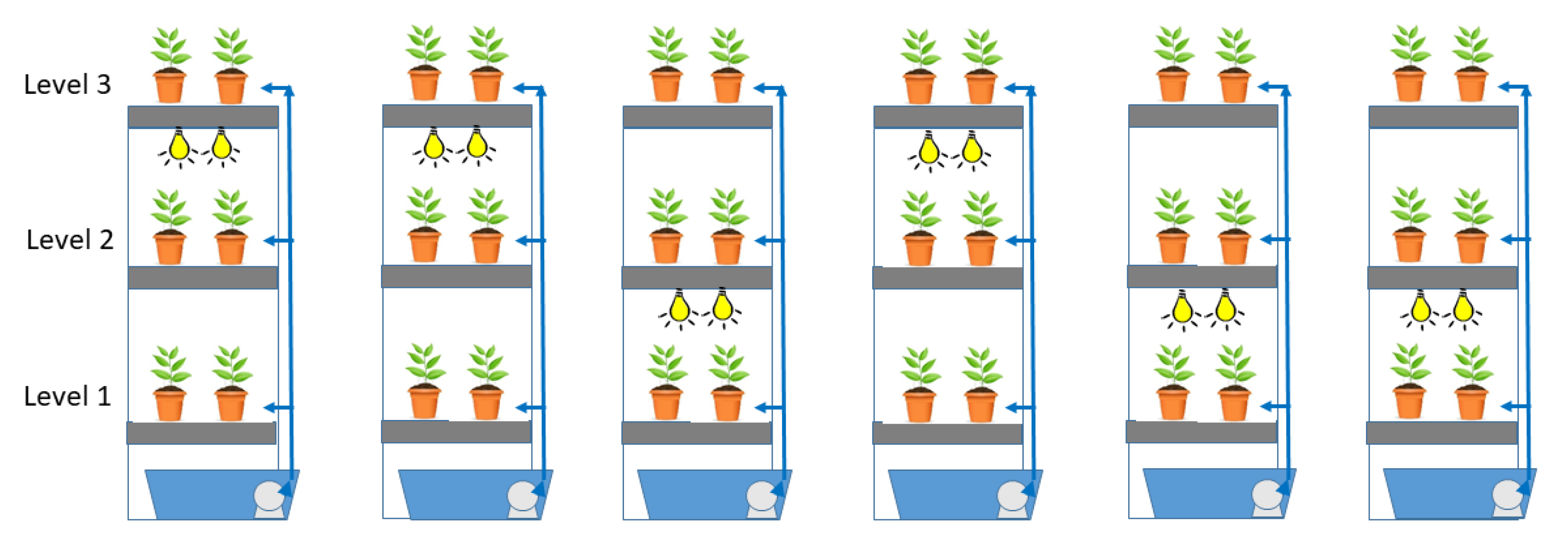
In this investigation, six decoupled aquaponic vertical racks were compared (Figure 1) to two horizontal systems (Figure 2). Each vertical rack was composed of three 1.22 × 2.44 × 0.15 m flood and drain trays (Botanicare, Chandler, AZ, USA), a 473 L sump filled with effluents coming from three 2000 L recirculating fish tanks, and a 4164 L h⁻¹ submersible water pump (ActiveAqua 1100 GPH, Hydrofarm, Petaluma, CA, USA). Each tray was irrigated individually (i.e., did not drain from one to the next), and flow was regulated with ball valves to have equal flow to fill all trays. These vertical rack systems were placed roughly 1.22 m apart and contained three shelves, with one of the two lower shelves receiving LED lighting distributions. Trays were spaced 0.61 m apart vertically, with shelving at the heights of 0.61 m (Level 1), 1.22 m (Level 2), and 1.83 m (Level 3). Trays were flood-irrigated twice a day, at 07:00 and 14:00, for 15 min using a timer connected to pumps, to a depth of approximately 0.02 m. All trays contained 200 individual plants, with a single plant per pot, forming a 20 × 10 grid.

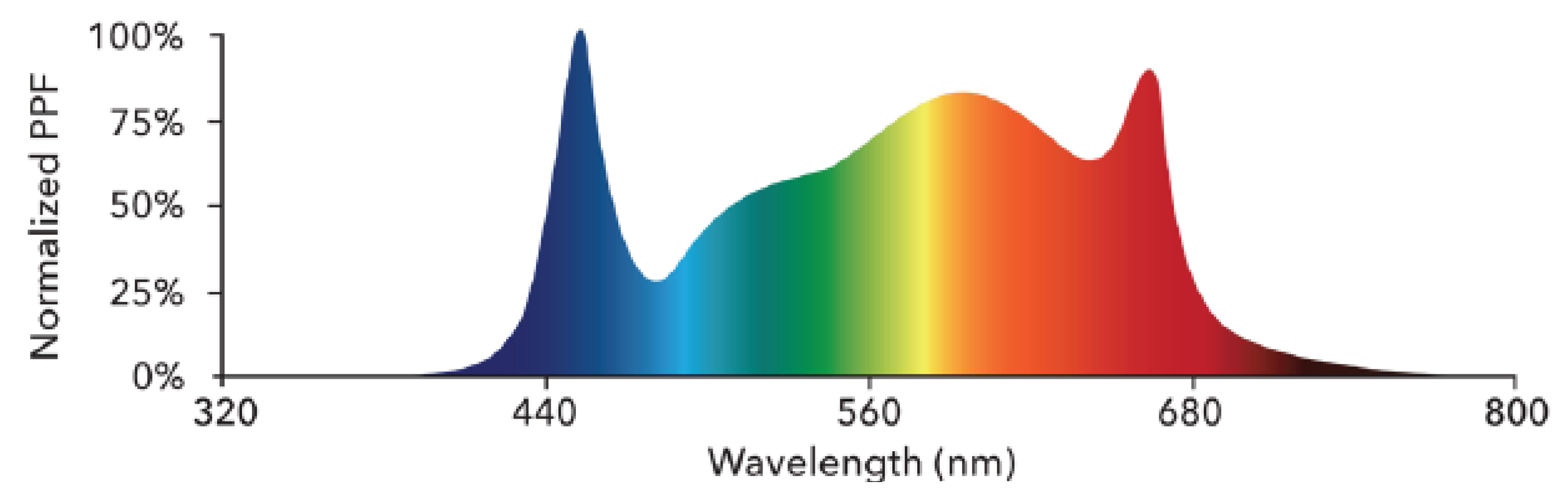
All top shelves were exposed to natural light, with the lower shelves with or without light supplementation by four Infinity 2.0 (Thrive Agritech, New York, NY, USA) LED light bars (1.2 m length, 65 W, 145 µmol s⁻¹ light output) or had only natural light. LED bars provided full-spectrum white light with peaks at wavelengths corresponding to blue and red (Figure 3). This assay design blocked for greenhouse location, shelf height, and lighting. The prescribed artificial light in the vertical systems was randomized by number generator to alternate one LED-supplemented and one sunlight shelf per rack at levels 1 and 2. Supplemental lighting operated 14 h per day, from 06:30 to 20:30.

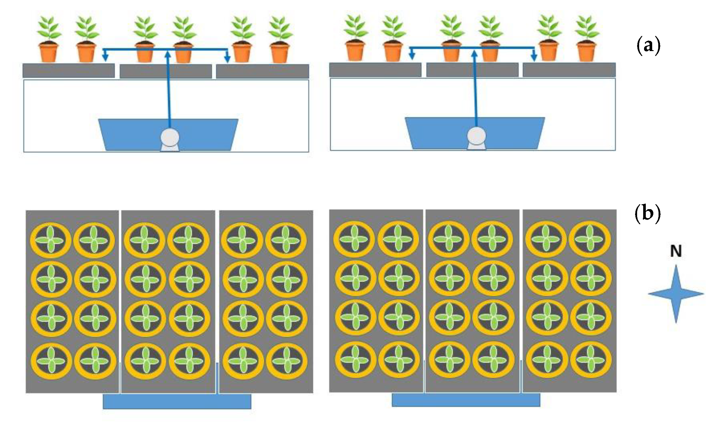
The two horizontal systems, located immediately east of vertical racks (Figure 4), consisted of the same equipment as vertical systems with identical trays (3 trays per rack), sumps, pumps, and irrigation periods. Plants in horizontal trays received natural sunlight only

The experiment was carried out from 19 August to 8 October 2019 in a 280 m² polycarbonate greenhouse located at UC Davis Campus (University of California, Davis, CA, USA; 38°32′18.8″ N 121°46′54.2″ W).

2.2. Fish and Plant Species

On the campus of the University of California, Davis (Davis, CA, USA), one of the products of interest is basil (Ocimum basilicum), widely used to make pesto sauce in different dishes on the daily menu for the Dining Commons. It is also a popular specialty herb that does well in commercial greenhouse production systems. For these reasons, basil was chosen as the plant species for this trial. However, since the available horizontal space limits the production of large commercial scale, vertical production was selected to compare the vertical growing systems’ effectiveness with that of conventional horizontal systems.

Basil is commonly produced using a multitude of commercial hydroponic growing methods that utilize an assortment of irrigation techniques. Commercial methods include the nutrient film technique (NFT), deep water culture (DWC), and, as was the case with this study, flood and drain methodology with pots filled with a soilless growing medium. Vegetable propagation trays (338S67S, Proptek, Watsonville, CA, USA) were filled with stabilized rooting media (Q plugs^®, International Horticulture Technologies, Hollister, CA, USA) and hydrated with reverse osmosis (RO) water. Pelleted seeds of Nufar Fusarium-resistant Italian large-leaf type basil (Johnny’s Selected Seeds, Inc., Winslow, ME, USA) were individually sown into each cell and placed into a flood and drain propagation rack. During germination, the propagation trays were irrigated with RO water twice a day for one hour (06:00–07:00 and 14:00–15:00). Fourteen days after germination, 4800 individual seedlings were transplanted into 0.102 × 0.102 × 0.089 m³ pots with ground Q plugs media and then placed into their respective systems at a density of 200 containers per tray (around 67 plants m⁻²). Each vertical rack system was supplemented with an additional 110 L of sturgeon effluent twice a week to replenish losses from evapotranspiration and maintain nutrient levels in the water.

Biological nutrients were sourced from the three recirculating aquaculture systems (RASs) located at UC Davis Center for Aquatic Biology and Aquaculture (CABA). White (Acipenser transmontanus) and green (Acipenser medirostris) sturgeon (<1 yr) were reared in 2000 L fish tanks on well water with mechanical and biological filtration occurring by bead filters. Tanks were fed 200 g daily of sinking complete feed for trout and steelhead (Skretting, Tooele, UT, USA) with 46% of crude protein, 12% of crude fat, 3% of crude fiber, and 1.1% of phosphorous. Water changes occurred twice a week by pumping 2200 L of filtered aquaculture tank water into a storage tank and transporting the water to the greenhouse.

2.3. System Operations and Measurements Performed

2.3.1. Plant Nutrient Supplementation

Aquaponic systems usually show low concentrations of K, Fe, P, or Ca in the water soluble fraction of fish effluents [10,11]. Therefore, the plants were visually examined to observe for the occurrence of nutrient insufficiency, and seedlings were prescribed a 1% KNO₃ foliar feed treatment. Plants were dosed in the morning twice a week with a manual sprayer with additional potassium without affecting the pH of the nutrient solution. Iron is also one of the essential micronutrients usually deficient in aquaponic systems due to its low amount in commercial fish feed [12]. Therefore, 0.2 g of chelated iron diethylene triamine pentaacetic acid (DTPA) (13% Fe) was dissolved weekly in the water of each sump, resulting in an increase in the Fe concentration of 0.055 mg L⁻¹. Thus, the total Fe applied to each system was 0.182 g, while the expectable Fe uptake by plants for optimum nutrition was estimated to be around 0.174 g. Fe–DTPA is assumed to remain in solution available to plants at the pH range of the solution in sumps. This calculation allows us to suppose that the Fe supply was enough to cover plant needs without increasing Fe concentration in sumps to toxic levels, an argument supported by the total absence of symptoms of internerval chlorosis. In this sense, crop needs were covered with increases in Fe concentration in sumps lower than that previously reported for basil production in the University of the Virgin Islands (UVI) system (2 mg L⁻¹ DTPA applied every 3 weeks) [13]. Hydroponic plant production is traditionally grown in a soilless medium with the majority of nutrients provided by an aqueous solution. In this study, all nutrients were provided by flood irrigation, supplied directly to saturate the root zone with the exception of potassium, which was applied via foliar spray.

2.3.2. Water Quality

Nitrate concentrations (ppm) were quantified weekly using a LaMotte^® Nitrate Nitrogen tablet testing kit (Chestertown, MD, USA) to maintain a concentration around 60 ppm (57.5 ± 18.4 ppm) in all systems after fish effluent replenishment. Weekly nitrate uptake in each sump varied across treatments and replicates. When low values were recorded, sumps were replenished with fish effluents to increase levels to the desired range, which in aquaponic systems is lower than that required for hydroponic systems [14]. Daily water temperature, pH, and electrical conductivity (EC) readings were recorded using a Bluelab^® combo meter (Bluelab Corporation Limited, Tauranga, New Zealand). A combination of phosphoric and citric acid (pH Down; General Hydroponics, Sebastopol, CA, USA) lowered pH to the desired 6.0–6.5 range.

2.3.3. Lighting Measurements

Photosynthetic photon flux density (PPFD) measurements were taken biweekly in the morning (8:00), afternoon (12:00), and evening (18:00), for the 20 selected pots in each tray, using a full-spectrum quantum meter (MQ-500; Apogee Instrument, Logan, UT, USA). Readings were performed at the current height of the plants to assess light exposure on the plants throughout the day and to quantify the difference between natural and artificial light sources at the different levels of shelves. Average light readings at each position were correlated with plant yield (weight, height, number of leaves, and number of nodes). Data collection at all plant locations (discussed in the next section) required, on average, 1.75 h.

2.3.4. Plant Yield

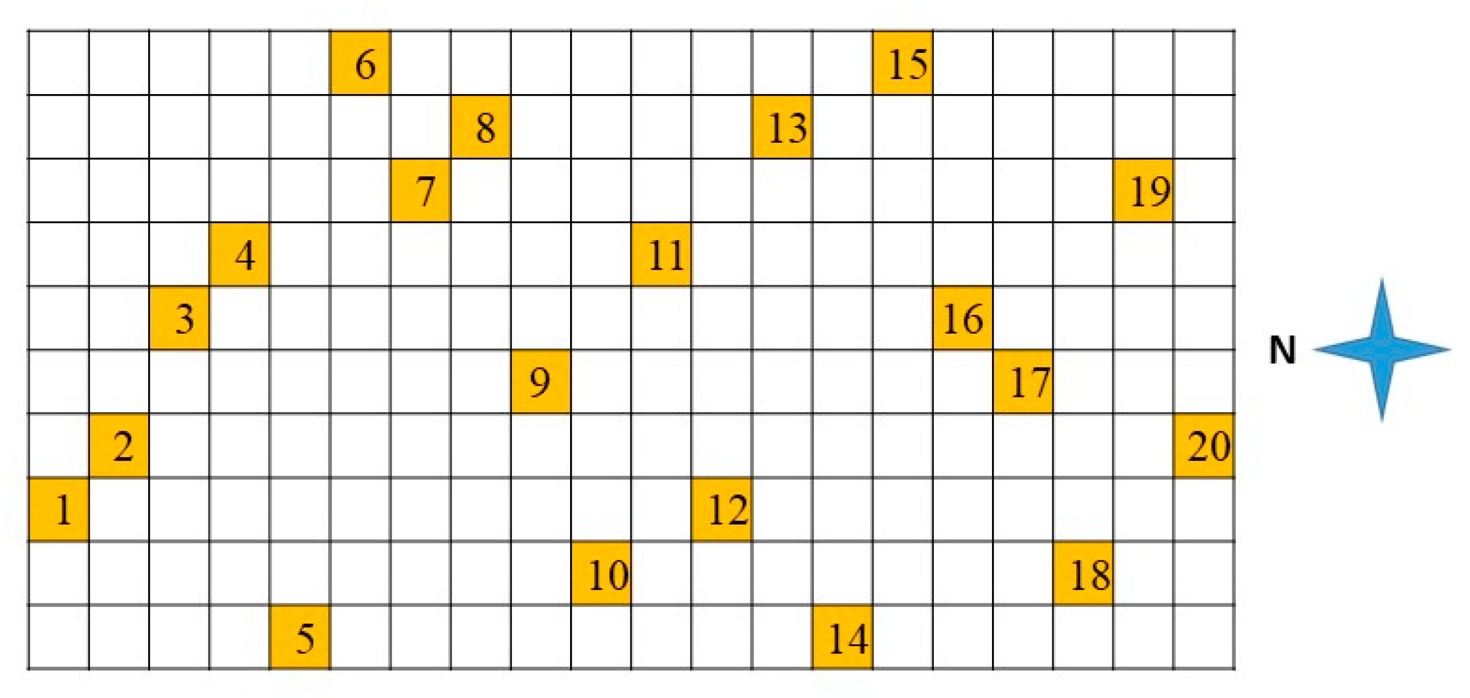
For each tray, 20 individual plant sites were monitored during plant development throughout the five-week study and examined biweekly for height, number of leaves, and number of nodes. Plant selection (Figure 5) was determined by dividing the tray of two hundred plants into two squares of 10 × 10 containers to account for potential variability of temperature with the proximity to the wet wall and of lighting. In each square, for consecutive positions in the north–south direction, a random value between 1 and 10 was generated. If the number was already selected, a new number was generated. Each square was treated independently so that only one pot was selected per line in the east–west direction, whereas two pots were selected in each line in a north–south direction. The same plant positions were selected for each of the 24 tray locations in this study. All basil, 35 days after transplanting (when lighting height was reached), was harvested at the base of the plant above the ground portion. The total biomass per tray was weighed, and 20 randomly predetermined plants per tray were weighed, measured, and the number of leaves and nodes quantified.

In order to prevent propagation error and to minimize experimental bias, a number of methods were conducted during the essay: (1) daily plant growth measurements and data recording were conducted by the same individual throughout the experiments; (2) final measurements and data recording were conducted by the same individual throughout the data collection experiments; (3) all data were recorded blind to LED treatments as final data collection was conducted in a separate room outside the view of the plant harvest; and (4) during data collection, the data recorder repeated and verified each record during the transcribing of data into a notebook, and all data recorded in the electronic spreadsheets were verified against the written copy to prevent input errors.

2.4. Statistical Analysis

Statistical analyses of the data were performed with the STATGRAPHICS Centurion XVIII statistical package (version 18.1.12, StatPoint Technologies Inc., Warrenton, VA, USA). For statistical comparison, a generalized linear model (GLM) was used. The normality of the data was assessed by means of the Shapiro–Wilk test. When data were not normally distributed, a nonparametric ANOVA (Kruskal–Wallis test) was used to confirm significant differences. Post hoc analysis was performed using the Honestly-significant-difference (HSD) Tukey test and the Games–Howell test (when variances were not equal). Differences were considered significant when p < 0.05.

3. Results

Average basil production recorded per unit area was 2.43 and 0.94 kg m⁻² for vertical and horizontal systems, respectively. Production per unit area in each of the trays was assessed to evaluate the differences between trays in different levels and lighting.

Basil production in trays located at tray level 1 showed significant differences according to lighting, with the highest values corresponding to shelves supplemented with LED, while no significant differences were found at level 2 (

Table 1. Mean values of basil production (kg m⁻²) in vertical racks according to tray level and lighting. Means with the same lowercase letter in each column and with the same capital letter in each row are not significantly different at the p < 0.05 level, according to the HSD Tukey test.

	Basil Production (kg m−2)
	Level 1	Level 2	Level 3	p
Sunlight	0.451 aA	0.685 aAB	0.981 B	0.0092
Sunlight + LED	0.750 bA	1.191 aA		0.0798
p	0.002	0.1106

). However, no significant differences were found between levels 1 and 2 for the same lighting conditions, although higher average values were obtained at level 2. Tray level 3 showed higher productivity than level 1, with only natural sunlight. Furthermore, comparing the production values obtained for levels 1 and 2 and taking into account only the height position (tray level) or the lighting mode (

Table 2. Mean values (± SE) of basil production (kg m⁻²) in levels 1 and 2 of vertical systems according to height and lighting. Means with the same letter in each column are not significantly different at the p < 0.05 level, according to the HSD Tukey test.

Lighting p = 0.0070	Production (kg m−2)	Height p = 0.0229	Production (kg m−2)
Sunlight	0.568 ± 0.087 a	Level 1	0.601 ± 0.087 a
Sunlight + LED	0.971 ± 0.087 b	Level 2	0.938 ± 0.087 b

), we found that both factors had a significant influence, while their interaction did not.

Production in the systems exposed to natural lighting found no significant differences (p = 0.6404) between the horizontal systems (0.939 ± 0.058 kg m⁻²) and the production obtained in the upper level of the vertical systems (level 3) (0.981 ± 0.064 kg m⁻²). When comparing production per unit area for each of the two types of systems studied (vertical and horizontal), significant differences were found in favor of vertical systems, as expected (

Table 3. Mean values (± SE) of basil production (kg m⁻²) in horizontal systems and vertical racks. Means with the same letter in each column are not significantly different at the p < 0.05 level, according to the HSD Tukey test.

	Basil Production (kg m−2)
Horizontal	0.939 ± 0.246 a
Vertical	2.427 ± 0.155 b
p = 0.0037

).

To more thoroughly evaluate factors of plant development in the horizontal and vertical systems, a GLM analysis was performed to determine the effect of the tray level, the lighting mode, and the position of the plant within the trays, using the data (weight, height, number of leaves, and number of nodes) obtained from the 20 selected basil plant individuals at harvest.

Similar to the analysis of productivity, a first study was carried out for tray levels 1 and 2 of the vertical systems where the level (1 and 2) and the type of lighting (natural or with LED supplement) were considered as categorical factors, while the distance to the north end of the tray (north–south direction) and the distance to the east end (east–west direction) were treated as quantitative factors. Out of quantitative factors, only the north–south direction showed a significant effect for all parameters, whereas both categorical factors were significant. The interaction between level and lighting system was also significant for all the parameters (

Table 4. Mean values (± SE) of weight, height, and number of leaves of 20 selected plants in vertical racks at levels 1 and 2. Means with the same letter in each column are not significantly different at the p < 0.05 level, according to the HSD Tukey test.

	Plant Weight (g)	Plant Height (cm)	Number of Leaves
Level 1 × Sunlight	7.13 ± 0.46 a	20.04 ± 0.55 a	9.30 ± 0.62 a
Level 2 × Sunlight	8.53 ± 0.46 a	26.13 ± 0.55 b	11.28 ± 0.62 a
Level 1 × LED	11.52 ± 0.46 b	20.48 ± 0.55 a	16.82 ± 0.62 b
Level 2 × LED	17.04 ± 0.46 c	33.23 ± 0.55 c	24.65 ± 0.62 c
Level × lighting	p = 0.0000	p = 0.0000	p = 0.0000
North-South direction	p = 0.0000	p = 0.0000	p = 0.0000

), except for the number of nodes (

Table 5. Mean values (±SE) of the number of nodes of 20 selected plants in vertical racks at levels 1 and 2. Means with the same letter in each column are not significantly different at the p < 0.05 level, according to the HSD Tukey test.

		Number of Nodes
Height p = 0.0000	Level 1	4.49 ± 0.06 a
	Level 2	5.22 ± 0.06 b
Lighting p = 0.0000	Sunlight	4.55 ± 0.06 a
	Sunlight + LED	5.16 ± 0.06 b
North-South direction	p = 0.0000

). Higher values for all parameters are associated with the upper level in trays and with LED supplementation, including now a positive effect for plants located at southern positions in trays. All results obtained for individual plant parameters seem to be consistent with those from productivity in trays. Nevertheless, due to the higher number of replicates and to the information related to the plants’ position in the trays, significant effects were found for categorical factors, their interaction, and the position of plants in the north–south direction.

The upper tray of vertical racks was again compared with horizontal trays using selected plant parameters at harvest. Even though no differences were obtained previously in the comparison of the productivities of the trays when the weights, heights, and number of nodes of the selected plants were analyzed, significant differences were found in favor of the vertical systems. There was also a significant effect of the north–south position on weight and height (

Table 6. Mean values (± SE) of weight, height, number of leaves, and number of nodes of 20 selected plants in trays of horizontal systems and level 3 (upper level) of vertical racks. Means with the same letter in each column are not significantly different at the p < 0.05 level, according to the HSD Tukey test.

	Plant Weight (g)	Plant Height (cm)	No. of Leaves	No. of Nodes
Horizontal	12.98 ± 0.30 a	31.58 ± 0.45 a	22.73 ± 0.50 a	5.70 ± 0.05 a
Vertical	13.97 ± 0.33 b	33.55 ± 0.49 b	24.06 ± 0.55 a	6.18 ± 0.05 b
System	p = 0.0293	p = 0.0033	p = 0.0745	p = 0.0000
North-South direction	p = 0.0177	p = 0.0468	p > 0.05	p > 0.05

). Only the number of leaves showed no significant differences in both systems.

Since differences in the intensity of the illumination affect plant growth and yield parameters, the mean values and standard deviations of PPFD records were calculated for the 20 positions of each tray.

Table 7. PPFD mean and SD values (µmol s⁻¹ m⁻²) were recorded at dawn, noon, and dusk at 20 selected positions per tray. Mean values were calculated by tray quadrant, namely north (samples 1 to 7), center (8 to 13), and south (14 to 20). V1, V2, and V3: Vertical trays at levels 1, 2, and 3, respectively. H: horizontal tray. SUN: only natural sunlight. LED: with LED supplementation.

			Dawn		Noon		Dusk		Average
Tray	Light	Position	Mean	SD	Mean	SD	Mean	SD	Mean	SD
V1	SUN	North	32.9	13.9	77.4	31.3	24.1	8.5	44.8	30.9
V1	SUN	Center	31.1	15.0	72.1	23.4	21.4	6.8	41.5	27.5
V1	SUN	South	44.7	18.7	183.3	110.1	43.3	42.7	90.4	95.1
V1	LED	North	170.5	40.8	208.2	29.7	142.6	39.2	173.8	45.5
V1	LED	Center	168.4	33.5	204.8	27.4	145.1	37.6	172.8	41.0
V1	LED	South	186.3	52.3	290.1	91.8	141.9	45.5	206.1	90.7
V2	SUN	North	57.9	16.1	101.0	26.8	19.1	14.9	59.3	39.0
V2	SUN	Center	57.8	16.2	97.4	19.6	17.1	9.8	57.4	36.4
V2	SUN	South	79.9	21.6	193.5	80.4	36.3	33.9	103.3	84.1
V2	LED	North	168.9	47.7	224.6	33.3	167.2	66.1	186.9	57.1
V2	LED	Center	165.0	34.7	216.2	25.9	161.9	48.5	181.0	44.8
V2	LED	South	170.9	48.1	280.6	67.2	164.3	58.3	205.2	78.9
V3	SUN	North	130.9	25.5	361.9	31.1	98.9	81.3	197.2	128.5
V3	SUN	Center	143.5	34.3	416.9	67.1	127.8	94.7	229.4	150.1
V3	SUN	South	154.2	38.5	467.8	49.4	117.4	80.7	246.5	168.2
H	SUN	North	408.1	274.2	399.0	87.5	23.2	3.8	276.8	244.3
H	SUN	Center	446.2	282.0	406.9	69.0	24.6	5.4	292.6	253.3
H	SUN	South	438.7	283.5	425.2	84.8	25.7	6.3	296.5	256.5

shows the values measured at dawn (8:00), noon (12:00), and dusk (18:00) with the average values from trays in horizontal and vertical systems separated by quadrant, namely north (samples 1 to 7), center (8 to 13), and south (14 to 20). Higher PPFD values are observed for the three selected times at higher levels, LED-supplemented trays, and southern positions in trays.

To evaluate the influence of illumination on yield, the average value of all PPFD readings were regressed with plant weight using a multiplicative model, and a significant correlation between both parameters (p = 0.0000) was found with a coefficient of determination of 0.52. The equation corresponding to the adjusted model is as follows:

ln(Weight) = −0.422383 + 0.571854 × ln(PPFD).

(1)

Adjustment with a multiplicative regression model was made as the recorded PPFD data had average values well below the 1600 µmol s⁻¹ m⁻² when saturation was reached.

To study the economic feasibility of lighting supply, the productivity of racks with supplemental lighting in tray level 1 (LED-1) and level 2 (LED-2) was compared with the estimated productivity of a simulated rack with and without supplemental lighting at both levels 1 and 2 (LED-1&2) (

Table 8. Productivity and lighting cost for extending production obtained using none, one, or two shelves with light supplementation in simulated racks. Sunlight: with no lighting. LED-1: supplemental lighting in level 1. LED-2: supplemental lighting in level 2. LED-1&2: supplemental lighting in levels 1 and 2.

	Simulated Racks
	Sunlight	LED-1	LED-2	LED-1&2
Level 3 (kg basil m−2)	0.981	0.981	0.981	0.981
Level 2 (kg basil m−2)	0.658	0.658	1.191	1.191
Level 1 (kg basil m−2)	0.451	0.750	0.451	0.750
Rack total production (kg m−2)	2.090	2.389	2.623	2.922
Lighting cost ($ m−2)	0	6.53	6.53	13.06
Value of production ($ m−2)	28.38	32.44	35.62	39.68
Increment of value ($ m−2)		4.06	7.24	11.30
Difference investment–return ($ m−2)		−2.47	0.71	−1.76
Cost per kg of production increment ($ kg−1)		21.84	12.25	15.70

). The lighting cost per unit area at each level was calculated considering an operating time of 14 h per day for 35 days. Each of the four LED bars used per shelf (2.973 m²) had 65 W of input power, and the considered average cost of electricity in California was 0.1524 $ (kWh)⁻¹ [15]. The economic value of basil production was estimated using an average price of 13.58 $ kg⁻¹ [16]. The cost of the increase in production was calculated as the ratio of the electrical cost of lighting and the increase in production.

4. Discussion

In the present study, we observed that for basil grown using flood and drain methods, the vertical system production per unit area was approximately 160% greater than the production obtained from the horizontal systems (Table 3). This production was lower than the 200% increment that could be expected considering three times the average production of horizontal trays per unit area (production using 3-level trays would mean obtaining an extra maximum yield of two trays compared to the yield obtained with a single horizontal tray). The difference in the added production, even with the reduced performance in the shaded tiers, supports the consideration of vertical agricultural production systems in urban or peri-urban environments, due to the high price of land.

Numerous published studies compare productivity between horizontal and vertical hydroponic systems. Higher productivities per unit area in vertical systems are always highlighted, as in our case. The magnitude of these differences is affected by the type of crop studied and the characteristics of these systems. Neocleous et al. [8] compared horizontal and vertical hydroponic systems for lettuce and strawberry. Lettuce, from the vertical system, achieved more marketable lettuce heads per system’s surface area compared to the horizontal setup. However, the horizontal system showed a greater average weight per plant and a higher percentage of marketable products. For strawberry production, the vertical arrangement presented a higher yield than the horizontal one. At the same time, the quality parameters did not differ between both systems, suggesting that variation based on those parameters is crop-dependent.

Similar findings were reported for strawberries by Ramírez-Arias et al. [9], who evaluated phenology, yield, and quality parameters of strawberry using three high-density hydroponic settings, i.e., two horizontal and one vertical (bucket columns). In this case, the average production obtained per plant was not statistically different between the vertical and horizontal systems, whereas the productivity per growing area in the vertical systems was 3.23-fold and 1.8-fold compared to the other two horizontal setups. Similarly, in this study with vertical racks, lower PPFD values were observed for the plants in the bottom level of the vertical systems, and lower yields were recorded. This fact seems to corroborate the conclusion that the influence of light supplementation has a more profound impact on lower trays, where the amount of light received by the plants is reduced due to shading.

Touliatos et al. [5] compared a vertical and a conventional horizontal hydroponic system with similar fertigation regimes, root zone volumes, and planting densities to determine the viability of an indoor vertical lettuce production but, in this case, only using artificial lighting. Again, a higher productivity for a vertical growing system (producing 13.8 times more lettuce per growing floor area than the same system in horizontal position) was reported, while quality parameters were inferior (the average fresh weight of the shoots was significantly higher in the horizontal setup). In their study, average plant weight decreased from top to base grow levels of vertical columns, with no gradient in productivity observed between levels in the horizontal system. A similar effect was found in our study. Furthermore, plants grown at the top layer of the vertical systems and within all trays of the horizontal setup showed similar average weight. Productivity decreased significantly for those at the middle and bottom layers of the vertical system in contrast to trays with full access to natural light. As a result, the bottom layer of the vertical system produced 43% less shoot fresh weight than the top layer. In parallel, it was observed that light intensity decreased significantly from upper to lower levels of vertical columns (from 224 to 122 μmol·m⁻²·s⁻¹).

In contrast, no significant difference in PPFD was observed within the horizontal and upper vertical layers (288-224 μmol·m⁻²·s⁻¹). As was reported in our work, there was a significant positive relationship between shoot fresh weight and PPFD in the vertical systems, indicating that as light intensity increased, so did crop productivity. In our vertical racks, there was also a gradient effect due to the position of the plant in the trays. The northern end of the trays, in addition to receiving less solar radiation due to the shading effects of neighboring shelves, was also closer to the cooling system (located between levels 1 and 2), as shown in Figure 4. This proximity caused a lower air temperature that affected the plants located in both growing modalities. For this reason, it is vital to characterize the factors specific to the growing environment that influence plant production (temperature and light, fundamentally) to adequately design the distribution of light sources at different levels of the vertical systems and the orientation of the trays within them.

Supplemental lighting will be required in vertical systems, as the intensity of light reaching the plants located at the bottom levels will always be lower than the one that reaches the plants in the upper levels in a greenhouse environment. Some argue that it would be too expensive to produce food indoors using artificial lighting [6]. However, the optimization and price reduction of LEDs opened a new stage for horticultural production as they allow a reduction of the production cost of vegetables in the long run, due to the LEDs’ high energy efficiency, low maintenance cost, possibility of wavelength selection, and lifespan [17].

The lighting distribution, as well as the use of more accurate digital controls for wavelength selection and intensity, increase the capacity to adapt the spectral distribution on each plant, adjusting to specific growth rates. LEDs can play an essential role in optimizing growth and producing high-quality vegetables by increasing not only the growth and yield of plants but also nutraceutical quality. Some light intensities increase the biosynthesis of pigments and improve the antioxidant content of the leaves or fruits. In this sense, the selection of LED primary light sources in relation to the peaks of the absorbance curve of plants is essential [18].

For a crop like the one used in this study, a high amount of light is required to maximize production. Liaros et al. [19] estimated that the necessary daily light integral (DLI) for the production of basil is approximately 15 mol m⁻² d⁻¹ that, with a photoperiod of 14 h d⁻¹, implies a PPFD of approximately 300 μmol m⁻² s⁻¹, which can be associated with high energy costs. Lighting then represents a considerable obstacle to producing profitable vertical systems. However, there is the possibility of compensating for high electricity costs, particularly for those plants that require more light by targeting higher-value crops [20]. In this sense, viable economic models were investigated in Greece which found that sweet basil, for example, was still commercially viable, despite the high light requirements because it had a higher value [19].

From a practical point of view, it would be interesting to know if the increase in harvest obtained with this additional lighting outweighs the added cost of lighting and energy expenditures. In the present work, a simple study of the costs was carried out, relating the expenses associated with different lighting distributions in vertical systems with the productive increases obtained with them. Accounting for the cost of electrical energy and the wholesale price for basil, it was concluded that the most cost-effective option would be to include lighting at the intermediate level of the shelves. Therefore, LED lighting will be profitable only when the price of the product in the market is over the differential electricity costs associated with the increase in production (Table 8). In our case, with the increment in production obtained in each scenario and the cost of electricity considered, the minimum price for the basil would be 12.25 $ kg⁻¹ (for the extra lighting in Level 2). However, depending on market variations (selling price of basil and on the electricity costs) and growing location, these conditions may vary, making other lighting distribution alternatives profitable.

The production per unit area (kg·m⁻²) is considered a useful indicator to be able to compare productivities in different systems. One of the classic literature references on aquaponic production is the work carried out in the Virgin Islands with commercial-scale systems (UVI system) [13]. In these systems, higher basil productivities were reported for the outdoor commercial-scale aquaponics systems in the tropics (1.8 kg m⁻²) than those obtained in soil (0.68 kg m⁻²). This reported yield in the aquaponics systems is higher than the one observed in our study for horizontal systems, likely due to differences in climate parameters in the tropics (ambient temperature, illumination, photoperiod, etc.) and, most importantly, because plants were harvested three times by cutting, before a fourth and final harvest. Results from other studies for horizontal aquaponic production of basil in combination with carp for 180 days and three subsequent harvests (939, 1130, and 1213 g m⁻²) with 600 W lighting supplementation were also consistent with those obtained with the UVI system [21].

There are also studies comparing aquaponic production with hydroponic production, although in these cases the results are highly variable. In the study carried out by Saha et al. [22], basil hydroponic production was compared with a crayfish-based aquaponic system in a greenhouse using floating rafts. The growth pattern and average plant height of basil at harvest were reported as 14% higher in aquaponics (89.9 ± 4.5 cm) as compared to that in hydroponics (78.7 ± 3.9 cm). The aquaponic system generated 56% more average fresh weight per plant (150.2 ± 18 g) than the hydroponic system (96.6 ± 10.4 g). Furthermore, the corresponding average dry weight for aquaponics (15.9 ± 2 g) was 65% higher than that for hydroponics (9.6 ± 1 g). However, in the study carried out by Roosta [23] for basil production in a greenhouse using different ratios of carp-based aquaponics and hydroponic irrigation solutions, the best results (a shoot fresh mass around 240 g per plant) were obtained with hydroponics. This study reported that when only irrigating with the aquaponic solution, approximately 50 g per plant were achieved.

When considering the information reviewed and the results obtained in this study, there are a series of elements that must be taken into account when evaluating the possibility of designing a vertical production system. In addition to the cost of the land for the installation, the most appropriate type of crop must be assessed. Although it is likely that, in all cases, a higher productivity will be obtained per unit area, there will be substantial differences in terms of product quality for different crops and the overall mass harvested, such as for crops capable of multiple harvests. Furthermore, not all plants are suitable for vertical production as the available height for plant development is limited [24].

5. Conclusions

From the data obtained on the production of basil in decoupled aquaponic systems configured in vertical and horizontal systems, it was found that, with simple maintenance operations, it is possible to increase productivity by 160% compared to that obtained per unit of surface in horizontal systems.

It was highlighted that one of the main limiting factors in vertical production is associated with low levels of natural light in the bottom shelves of vertical systems, which must be compensated with additional lighting. However, the associated higher lighting costs to improve production yields must be considered. One potential solution to this problem would be to select crops with lower light requirements and higher prices in the market.

Finally, it is necessary to emphasize the importance of facility design, not only in relation to the distribution of light sources but also for the correct adjustment of the uniformity of temperature values to homogenize the environmental parameters associated with plant growth.