Article

Improving the Sustainability and Profitability of Oat and Garlic Crops in a Mediterranean Agro-Ecosystem under Water-Scarce Conditions

by
José Antonio Martínez-López
1,
Ramón López-Urrea
2,
Ángel Martínez-Romero
1,
José Jesús Pardo
1,
Francisco Montoya
1,2 and
Alfonso Domínguez
1,*
1
Centro Regional de Estudios del Agua (CREA), Universidad de Castilla La Mancha (UCLM), 02071 Ciudad Real, Spain
2
Instituto Técnico Agronómico Provincial de Albacete (ITAP), Parque Empresarial Campollano, 2a Avenida No 61, 02007 Albacete, Spain
*
Author to whom correspondence should be addressed.
Submission received: 17 June 2022 / Revised: 28 July 2022 / Accepted: 17 August 2022 / Published: 18 August 2022
(This article belongs to the Special Issue Modernization and Optimization of Irrigation Systems)

Abstract

:
In areas with scarce water resources, population growth and climate change scenarios will mean that there is increasingly less water available for agricultural activity. Thus, optimizing crop irrigation water management is an absolute necessity. To address this situation, the SUPROMED project (sustainable production in water-limited environments of Mediterranean agro-ecosystems), available in an online platform, brings together a series of models and methodologies designed to promote more efficient management of water, energy and fertilizers. A two-year trial (2020–2021) was implemented in the Castilla-La Mancha region (Spain), with the aim of showing the effectiveness of SUPROMED as a farm management support tool. The trial was conducted on two of the region’s most important crops (oats and garlic). A series of productive, economic, and environmental key performance indicators (KPIs) were analyzed to measure the impact of transferring MOPECO (model for the economic optimization of irrigation water use at farm level), the irrigation scheduling model integrated in the SUPROMED platform, to farmers. In 2020, the management plan proposed by SUPROMED achieved a higher yield for oat than that generated by traditional management, using 40% less water. In the case of garlic, the same yield was obtained, using 30% less water. Gross margin and gross economic irrigation water productivity were improved for both crops. In 2021, one of the selected farmers was trained to use the SUPROMED platform to work with garlic crop. This management improved most of the KPIs analyzed compared to previous management without the SUPROMED platform, obtaining similar results to those obtained by SUPROMED in 2020. The results demonstrate that the tools and models included in SUPROMED have been properly adapted and can be easily used by farmers, improving the economic and environmental sustainability of Mediterranean agroecosystems.

1. Introduction

The Mediterranean region is strategically located at the intersection of three continents. This area has a great diversity of animal and vegetal species across very varied and different ecosystems. However, climate change, which is causing the irregular distribution of rainfall [1] and periodic droughts, is threatening the area, especially the farming sector. The Mediterranean farming industry is also conditioned by the progressive increase in energy prices (about 3% per year since 2008 and more than 30% in 2020–2021 [2]), fertilizer prices, labor costs and legislation. This situation has deteriorated the economic environment and increased the risk of the end of agricultural activity, causing rural areas to be abandoned. To avoid this, proper governance of natural water resources is essential to ensure the economic, social and environmental sustainability of Mediterranean agriculture. In this sense, tools and management strategies are key to achieve this objective. Determining the irrigation requirements of crops at farm level can help improve efficiency in the use of irrigation water. Proper knowledge, management and maintenance of the irrigation system are as important as the correct determination of irrigation requirements in making more efficient use of water. Nevertheless, the excessive use of means of production (mainly water and energy) has become a frequent technique among traditional farmers to cope with the increasingly unpredictable weather, a result of climate change, which negatively affects the environment and the profitability of their farms [3,4].
Many techniques that can help make more efficient use of the means of production in agriculture are already available (e.g., climatic sensors, remote sensing-based approaches, soil moisture sensors, pressure transducers, flowmeters and physiological measurements). However, in many cases, they are not used by farmers due to their high implementation cost, the complexity in data interpretation, their correct implementation in decision-making, etc. For this reason, it is necessary to adapt and transfer these techniques to producers in a simplified way that allows them to make the most suitable decision in the correct time, improving the resilience of agricultural systems [5].
As a decision support system for farmers and/or technicians, crop simulation models can help achieve this. Several such simulations models have been developed [6,7,8,9] but most require a large number of parameter values that are not easily accessible to farmers. The MOPECO model (model for the economic optimization of irrigation water use at farm level) [10] maximizes the gross margin of farms through more efficient use of irrigation water. The MOPECO model optimizes farm water management and identifies the proper crop rotation, optimizing economic and yield water productivity and minimizing the environmental impact [11,12,13]. The main advantage of MOPECO is that it generates irrigation schedules according to the total available irrigation water in a user-friendly way, while considering complex concepts [13,14,15]. The farmers only need to insert the data from their farms and select their crops from a list of calibrated crops, mainly for the Castilla La Mancha region (CLM—Spain) (maize [13,16], onion [17], garlic [18,19], barley [20,21], potato [22], melon [23]), but also for other countries [23,24].
MOPECO is implemented in the online platform of the SUPROMED (sustainable production in water-limited environments of Mediterranean agro-ecosystems) project, designed to improve the economic and environmental sustainability of Mediterranean farming systems. SUPROMED also includes other models and tools, such as PRESSUD (pressurized subunit design) [25] and DOPIR (design of pressurized irrigation) [26] to improve the design of irrigation systems to achieve the proper management of inputs. Moreover, the project proposes several complementary methodologies, such as evaluation of the irrigation systems, control of the actual amount of irrigation water supplied at each irrigation event, monitoring the soil moisture content, and fertilization plan calculated according to soil analysis and nutrient balance. These complement the models included in the online platform (www.supromed.eu accessed on 2 June 2022).
Oats, with more than 25 million of Mg produced annually worldwide [27], are an essential foodstuff for ruminants, which are widespread in the Mediterranean basin. It is a crop with notable social repercussions for small- and medium-sized farms. Together with barley, it is an essential crop within the typical agricultural systems in the area. Additionally, garlic, with more than 28 million of Mg produced annually in the world, is ranked 14th in areas dedicated to vegetable crops [19]. In Spain, Castilla-La Mancha (CLM) is the largest producing region (60% of the national total production [28]), with this sector being of great economic and social significance. Although both crops can positively contribute to the local economy of rural areas, tools and models are needed to perform adequate irrigation scheduling, avoid water percolation and make efficient use of water and other means of production to enhance sustainability.
The objective of this work was to demonstrate the impact of applying the SUPROMED models and methodologies on the sustainability and profitability of oat and garlic crop in comparison with the traditional management of these crops in the Castilla-La Mancha region (Balazote and Albacete, Spain). The following partial objectives were proposed: (1) to determine a set of productive, economic, and environmental key performance indicators (KPI); (2) to monitor several farms dedicated to the cultivation of both crops and manage a subplot within one of the monitored farms, using the SUPROMED methodologies; (3) to train one of the farmers in the use of the methodologies in SUPROMED and monitor the management of the crop during a second year; and (4) to compare the monitoring results using the KPIs.

2. Materials and Methods

The study was carried out under the framework of the European project SUPROMED “GA-1813” funded by PRIMA, similar to the paper previously published by [29], which can be consulted in open access.

2.1. Field Experiments

The field trials were conducted in 2020 and 2021 in different commercial plots of oats and garlic, located in the Castilla-La Mancha (CLM) region (Spain). CLM is one of the three demo sites in the SUPROMED project. This is a semi-arid climate region, where the average annual temperature is around 14 °C, and the accumulated rainfall is between 200 and 400 mm year−1 (recorded mainly in spring and autumn). The average annual reference evapotranspiration is around 1300 mm year−1, varying between 30 and 220 mm month−1 in January and July [19]. In general, in CLM, the average soil depth is between 40 and 60 cm, finding a petrocalcic horizon. Additional information is available in [29].

2.2. Monitored Plots

In order to compare traditional management and that proposed by SUPROMED (SUP), several plots belonging to different farmers were selected. One of the farmers was selected as a “Leader” farmer (LEA), being one of the best-trained and highest-producing farmers in the area. Consequently, two plots on his farm, with similar characteristics, were monitored: one managed by LEA and the other by SUP. The other selected farmers were producers, whose training and production methods are typical of the area (AVE).
In each monitored plot, the area delimited by a set of four sprinklers representing the average conditions of the sector was selected to monitor the experiments.
Before sowing, the soil profile of each commercial demonstration plot was sampled to determine the effective soil depth and physical (texture) and chemical (nutrient content) properties. Soil analyses were used by MOPECO to determine the irrigation scheduling and fertilization by SUP management and to simulate the farmers’ irrigation schedules.
In the 2019–2020 season, three oat plots of (Avena sativa L., cv. Chapela) from two different farmers were monitored (Table 1). The variety of oats is a fodder crop but considering the rainfall forecast in the moment of fodder harvest, the farmers decided to leave the crop to produce grain, because this rainfall would have affected the fodder quality, resulting in significant economic losses. However, a portion of the plot was also harvested to determine the hypothetical yield that would have been achieved as fodder.
Furthermore, in the 2019–2020 season, four plots of garlic (Allium sativum), three plots of cultivar Violet Spring and one of cultivar Morado de las Pedroñeras from three farmers were monitored. However, in the 2020–2021 season, only two plots of spring garlic were monitored. One of these was managed by the leader farmer using SUPROMED (LEASUP), to quantify the improvement capacity of using the platform (https://dss.supromed.eu accessed on 2 June 2022). The other plot was managed by AVE 1. In addition, another plot of Morado de las Pedroñeras was monitored in this season (Table 1).
A petrocalcic horizon was found in all cases, which limited the useful soil depth. In the oat plots, the texture was clay-loam and the pH was basic (8.5). The soil depth was 55 cm for AVE 1 and 50 cm for SUP and LEA. AVE 1 had less organic matter than SUP and LEA (1.96% vs. 2.15%), with the latter having a higher carbonate content (39.77%) and active limestone (11.32 %) than AVE 1.
For the garlic crop, average soil depth was 40–45 cm, being classified as clay-loam texture, except for AVE 2 (loamy-sand texture in 2020 and sandy-clay-loam texture in 2021). The soils are basic (pH varied between 8.4 and 8.6).
For SUP and LEA plots, the farmer applied sheep manure to reduce the amounts of mineral fertilizer. This resulted in a higher organic matter content compared to other plots, (reaching 2.6%). In 2020, SUP and LEA plots presented higher carbonate content (43.4%) and active limestone (12.6%) compared to AVE 1 (40.7% of carbonates and 12% of active limestone). In 2021, AVE 1 presented the highest carbonate and active limestone values (42.2% and 12%, respectively).
In 2021, the AVE 2 soil had 12.55% of carbonates and 6.41% of active limestone, being better than the soil in 2020 (41.95% of carbonates and 11.55% of active limestone).

2.3. Irrigation System

In 2020 and 2021, AVE 2 plot was irrigated by using a center pivot system (Table 2). In the eight remaining monitored plots, a fixed solid set sprinkler irrigation system was used. Before the start of the campaign, each irrigation system was evaluated to characterize the spatial distribution of the water applied by the irrigation system, and to determine the actual amount of water applied at each irrigation event at working pressure.
All this information was used by the SUP team to calculate the proper irrigation scheduling and to improve the irrigation uniformity of the SUP plot, if necessary.
The (fixed) solid set sprinkler irrigation system was evaluated using the methodology proposed by [30] considering the established standards [31]. The methodology proposed by [32] was used for the evaluation of the center pivot irrigation system.
To compute the soil water balance using the MOPECO model, a general irrigation application efficiency of 80% was assumed in all cases. This value was based on values for Christiansen’s coefficient of uniformity (CU) obtained in the evaluations of the irrigations systems (most of them between 70 and 87%, Table 2), and on the low evaporation and drift losses considered due to irrigation events typically occurring during the night.
Table 2. Characterization of monitored irrigation systems.
CropCrop ManagementSprinkler Spacing
(m × m)
Pressure
(kPa)
Sprinkler
Discharge
(L h−1)
Application Rate
(mm h−1)
DU (%)CU (%)
Oats (*) SUP 17.3 × 17.3 398 2083 6.9 75.7 85.9
LEA 17.3 × 17.3 398 2049 6.9 77.8 87.4
AVE (1) 17.3 × 17.3 (1) 309 1839 (1) 6.1 (1) 76.5 86.7
Garlic (*) SUP 17.3 × 17.3 404 2003 6.7 79.4 86.1
LEA 17.3 × 17.3 404 2003 6.7 79.4 86.1
AVE 1 18 × 17.7 189 1544 4.8 54.8 70.73
AVE 2 25 ha (2) 500 143,280 According to speed 56.1 85.6
Garlic (**) LEASUP 17.3 × 17.3 403 2053 6.9 75.7 85.9
AVE 1 17.3 × 16.8 366 2109 7.0 76.5 86.7
AVE 2 30 ha (2) 380 179,640 According to speed 72.8 86.8
Where: SUP: Supromed; LEA: Leader; AVE: Average; LEASUP: LEA using SUP platform; DU: distribution uniformity; CU: Christiansen’s coefficient of uniformity. (1) Due to the lockdown imposed under the COVID-19 pandemic on March 15, these evaluations were not carried out. Estimated DU and CU values were included. (2): Area of the pivot irrigation system. (*): 2019–2020 campaign; (**): 2020–2021 campaign. Phenological stage: the BBCH scale [33] was selected to monitor the crop phenology during the two experimental seasons.

2.4. Irrigation Scheduling and Soil Water Monitoring

Daily irrigation scheduling was performed, using the simplified water balance methodology in the root zone [34,35], which is that used by MOPECO [15]. The tool known as “Irrigation Scheduling-MOPECO” (IS-MOPECO) was used (https://crea.uclm.es/siar/siarpr/ accessed on 2 June 2022). It requires climate (daily precipitation, ETo and mean temperature), soil (depth and texture), and crop data (Table 3).
Temperature, humidity, and wind data were recorded using an automated weather station IMETOS 3.3 (Pessl Instruments: Weiz, Austria), positioned at no more than 1 km from the monitored plots, and precipitation was collected at each plot.
Actual data are used to calculate irrigation scheduling in the past, and National Institute of Meteorology [36] predictions or typical meteorological year (TMY) [18,37] data are used to calculate irrigation scheduling in the future. Irrigation and precipitation events can be modified manually, and the program recalculates the soil water balance. Additional information is available in [29].
Table 3. Crop parameter values used by Irrigation Scheduling—MOPECO software for oats and garlic crop.
StageKcPhenological StageCGDD *Other
Parameters
Value
OatsI0.300–21450ET group3
II0.30–1.121–391045TL * (°C)2
III1.139–831596TU * (°C)30
IV0.383–891850
GarlicI0.700–14542ET group4
II0.70–1.014–411896TL * (°C)0
III141–472387TU * (°C)45
IV0.647–492671
Kc: crop coefficient values used by the irrigation advisory service of CLM (SIAR) based on those proposed by FAO 56 and fitted to the regional conditions [34,38]; Kc (I): initial; Kc (II): crop development; Kc (III): mid-season; Kc (IV): late season; 00: first day after sowing, dry seed; 14: 4th leaf clearly visible; 21: beginning of tillering: first tiller detectable; 39: flag leaf stage: flag leaf fully unrolled, ligule just visible; 41: leaf bases begin to thicken or extend; 47: 70% of the expected shaft length and diameter reached; 49: bulb top dry, growth complete; 83: early dough; 89: fully ripe: grain hard, difficult to divide with thumbnail [33]; CGDD: cumulative growing degree day [39]; ETgroup: evapotranspiration group, this conditions the fraction of the total available water (TAW) that a crop can extract without suffering water stress [40]. TU is the upper developmental threshold temperature or the temperature at and above which the rate of development begins to decrease; TL is the lower developmental threshold temperature or the temperature at and below which development stops. * CGDD, TL and TU values of both crops were calibrated for this work using the crop monitoring dataset provided by the CLM irrigation advisory service (SIAR).
In each plot, a soil moisture probe with 6 sensors at 10 cm spacing (Drill&Drop, Sentek: Stepney, Australia) was installed in a representative area according to the results of the irrigation system evaluations, to monitor the evolution of the volumetric soil water content. The average daily volumetric content according to the probes was transformed to available water and compared to those simulated by the MOPECO tool.
To monitor the duration and the water applied in each irrigation event, several devices were installed, depending on the irrigation system type. For the solid set sprinkler irrigation system, a pressure transducer (Pessl Instruments Pipe Pressure: Weiz, Austria) was installed in the rise of the pipe of the representative sprinkler. In center pivot plots, anARG314 rain gauge (ARG314, Campbell Scientific: Logan, UT, USA) was installed in a representative area of the center pivot, which showed a good uniformity of water distribution, according to the results of the irrigation system evaluations.
The rain gauge/pressure transducer and the probe were connected to a data logger (ECO D3, Pessl Instruments: Weiz, Austria).

2.5. Yield, Statistic Analysis and Key Performance Indicators (KPIs)

Once the crop reached physiological maturity, six 0.5 m × 0.5 m random samples were collected in the control area of each monitored plot to determine the yield. For the oat crop, grain yields were normalized to standard commercial yield (12% moisture content). In 2020, Duncan’s test [41] was performed to determine whether significant differences (p < 0.05) existed between different managements. Upon this comparison, we calculated various key performance indicators (KPIs), which can determine the efficiency in agronomic, and consequently in economic and environmental terms, of the different management systems [42,43,44,45]. The KPIs used were gross margin (GM), measured in euros obtained from the harvest per ha; irrigation water productivity (WPI), expressed in kg of yield per m3 of irrigation water applied; crop water productivity (WPc), as kg of yield per m3 of water evapotranspirated; net economic irrigation water productivity (NEWPI), as euros of GM per m3 of net water (irrigation and rainfall); gross economic irrigation water productivity (GEWPI), as euros of GM per m3 of gross irrigation water; and agronomic productivity of nitrogen (APN), as kg of yield per nitrogen units applied in one ha. In addition, the green, blue and grey components of the water footprint (WF) of the process were determined [44,45,46]. Additional information is available in [29].

3. Results and Discussion

3.1. Evaluation of the Irrigation System

All the irrigation systems of oats plots had a good distribution uniformity (DU) (Table 2), being adequate for proper irrigation scheduling.
For the garlic crop, the SUP and LEA plots reached the highest values of DU, with their being correct for proper irrigation scheduling. On the other hand, in 2020, AVE 1 had a poor DU value, because the working pressure of the irrigation system was lower than the normal pressure provided by the collective irrigation network. This was due to a large number of farmers irrigating at the same time, since the cost of electricity was lower (i.e., at the weekend) when the irrigation system was evaluated.
In the case of AVE 2, the irrigation system of which was a center pivot system, the DU computed from the evaluation was deficient (56% of distribution uniformity). The evaluation allowed us to identify several sprinkler problems, which were resolved after the evaluation.

3.2. Soil Analysis and Fertilization Requirements

SUP used the methodology proposed by [47,48] to calculate the crop requirements, taking into account the soil analysis and the information related to the previous crop.
For the oat crop, LEA applied 23% and 67% less N and K2O, respectively, but 147% more P2O5 than SUP, as he used a different mixture of fertilizers (Table 4). On the other hand, AVE 1 applied 96% more N compared to the calculated values, despite his calculated values being slightly lower than the SUP and LEA plots, because the previous crop for AVE 1 was maize, which left a great amount of crop residues, reducing the calculated values. For SUP and LEA, the previous crop was garlic, which left no residues.
For garlic, LEA applied 75% less K2O than SUP (Table 4). Both used sheep manure as a basic dressing fertilization that completed part of the crop requirements, but LEA applied no more K2O in the rest of the crop cycle. AVE 1 applied sheep manure as a basic dressing fertilization and completed the nitrogen crop requirements during the rest of the crop cycle.

3.3. Crop Development

For both crops, the length of the crop growth cycle was the same for the SUP and LEA management plans (Table 5). The difference between SUP and LEA was the irrigation scheduling and the amount of fertilizer applied. This had no effect on crop development, with both management schedules reaching the phenological stages at the same date.
The typical sowing dates for oat crops in the area were in autumn (Table 5), to guarantee a suitable biomass production of the crop and to improve rainfall water use. The harvest date for fodder oats is when the grain is in the early dough stage, which appears to generate the best combination of moisture, nutrient content and yield [49]. Up to this date, the crop accumulated an average of 1494 CGDD and 1851 CGDD, considering the crop cycle for grain use.
For garlic, in both growing seasons, the preferred garlic sowing date was mid-September in the case of cultivars with a long cycle (i.e., cv. Violet spring grown around 250 days in SUP, LEA and AVE 1 plots), while AVE 2 chose a short cycle cultivar (cv. Morado de las Pedroñeras grown in around 140 days (Table 5).
During the first year, the spring garlic crop was calibrated in terms of CGDD; an average of 2671 CGDD was calculated. During 2021, the spring garlic crop accumulated an average of 2552 CGDD (4% lower than the calibrated values the previous year).
Purple garlic accumulated an average of 2129 CGDD, being very similar to that calibrated (2044 CGDD) by [18].

3.4. Irrigation Scheduling

These results can only be compared directly in the case of SUP and LEA crop managements because both were obtained on the same farm and under similar conditions.
The ETa (crop evapotranspiration) of SUP and LEA crop managements reached ETm (maximum crop evapotranspiration), meaning that both management schedules avoided water deficit. Nevertheless, SUP achieved this with 38% and 33% less gross irrigation water than LEA for fodder and grain oats, respectively (Table 6), avoiding percolation of irrigation water and reducing total percolation by 38% compared to LEA. Consequently, this excess of irrigation water applied by LEA caused the percolation of irrigation water (around 35% of total percolation). This finding is simulated by the MOPECO model in Figure 1b, when the available water (AW line) surpassed field capacity (AW = 1). The possible reason for this finding is that the LEA farmer attempts to store as much water as he can in the soil because, in some years, if the climatic conditions are very dry, the irrigators’ community decreases the amount of available irrigation water and crops can suffer water stress. Thus, the rainfall at the end of March caused great percolation. On the other hand, AVE 1 applied the lowest amount of gross irrigation water (Table 6), ceasing to irrigate from the last period of the reproductive stage until the end of the crop cycle, suffering a severe water deficit that reached 0.85 ETa/ETm during the reproductive stage (the most sensitive stage to water deficit in cereals [50,51,52]) and 0.25 ETa/ETm during the last stage of the crop cycle. This is shown in Figure 1c, when the AW line in the MOPECO model, which ranges between the wilting point (AW = 0) and field capacity, crosses the allowable depletion level (deficit line).
For the garlic crop, in the first year, AVE 2 applied the lowest amount of gross irrigation water (277 mm). It should be noted that despite being a shorter cycle (Table 5), the amount of irrigation water is quite different with respect to the other management schedules because harvest occurs in June instead of May, coinciding with the period of highest evaporative demand (Table 7). Meanwhile, LEA applied the highest amount of irrigation water with 418 mm (Table 7).
Considering spring garlic (SUP, LEA and AVE 1 crop management) except SUP, all management schedules applied an excess of irrigation water, especially at the beginning of the crop cycle, to ensure good nascence. This caused the percolation of irrigation water (Table 7) and also the percolation of rainfall at the beginning of crop development and during the rainfall period at the end of March (Figure 2b,c). However, SUP, using MOPECO, applied 30% less gross irrigation water than the LEA farmer, avoiding the percolation of irrigation water and reducing rainfall percolation (Table 7). It is worth highlighting that, except in the case of AVE 2 (purple garlic), the ETa did not reach ETm in the last growing stage. This meant that the crop suffered a slight deficit at ripening, making it necessary to improve the harvesting work, but without a great impact on the final yield [18,53,54] (Figure 2).
During the second year, the LEA farmer learnt the techniques implemented by SUP in the first year and especially how to use the MOPECO irrigation scheduling tool. Another garlic plot was managed by the LEA farmer in 2021 in collaboration with the SUP research team (LEASUP). Despite the lower amount of rainfall, the amount of irrigation water decreased by 17% with respect to LEA 2020 (Table 7). Rainfall percolation was lower because the rainfall distribution was more homogeneous (Figure 2d). The amount of percolated water was reduced by 56%, compared to LEA in 2020. However, percolation could have been lower because, due to the uncertainty of rainfall forecast, an irrigation event to apply fertilizers at the end of December could have been avoided (Figure 2d). Nevertheless, the crop water requirements were satisfied, reaching a similar ETa/ETm., maintaining the soil moisture at a level that allowed rainfall and reduced percolation to be taken advantage of. On the other hand, AVE 1 obtained similar values to those obtained in 2020 with a similar amount of percolated irrigation water but lower rainfall percolation.

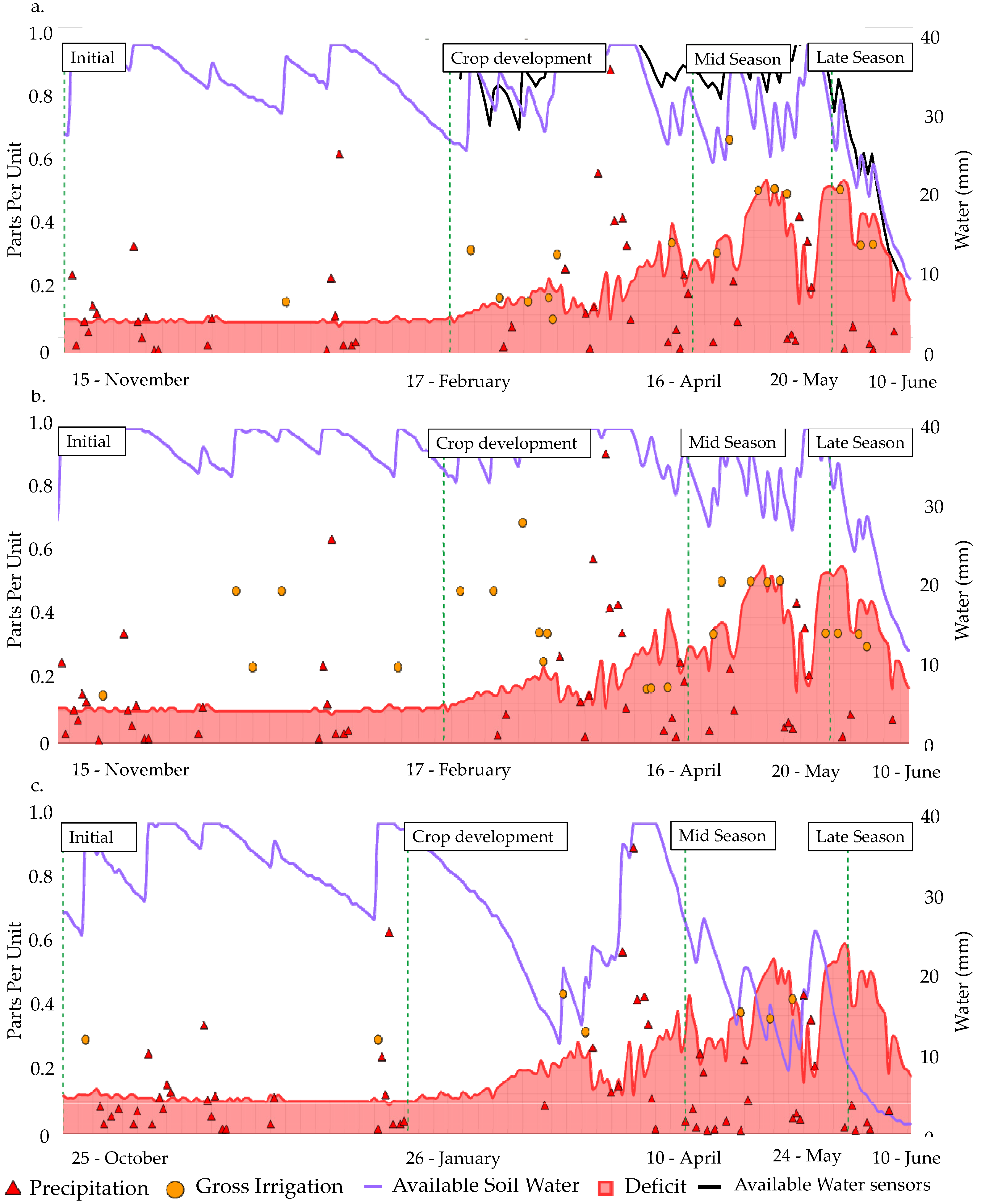
3.5. Soil Water Monitoring

For both crops, the pressure data obtained by the pressure transducers were used to determine the actual amount of water applied at each irrigation event (represented as orange dots in Figure 1 and Figure 2). These data were used to update the soil water balance of the MOPECO tool (Figure 1 and Figure 2), adapting the irrigation scheduling to actual irrigation events and simulating percolation if it existed. The irrigation scheduling was corroborated by the actual volumetric soil moisture data provided by the probes (i.e., SUP (2020) for oat crop (Figure 2a) and LEASUP (2021) for garlic crop (Figure 2d)). Therefore, the simulated soil water content could be expected to be representative of actual data for these crops in the area.

3.6. Analysis of Key Performance Indicators

All the management types for oat crop (fodder and grain oats) that suffered no significant water deficits (SUP and LEA) (Table 6) achieved similar yields, except AVE 1, which was lower (Table 8) (around 22%), This is because a moderate water deficit was caused during the third stage of the crop cycle (one of the most sensitive stages to water deficit [52]) and there was a severe water deficit in the last crop growth stage of the grain oats cycle (Figure 1c). Although SUP applied about 40% less irrigation water (Table 6), it obtained about 14% and 10% higher yield than LEA for fodder and grain oats. The possible cause of this was the lower amount of fertilizer (N and K) applied compared to the SUP treatment, which calculated the fertilization plan according to soil analysis (Table 4).
These differences in the amount of irrigation water and nitrogen applied affected the nitrogen productivity (APN) because, except for AVE 1, there were no differences between yields. Thus, LEA achieved the highest APN, improving on the result obtained by AVE 1 by 122% and 133% for fodder and grain oats, respectively (Table 8). These values are also 14% and 19% higher than SUP, because the drop in yield compensated for the lower amount of N applied (Table 8). SUP reached high WPc and WPI values (83 % and 66% higher than LEA), being surpassed only in WPI by AVE 1, because, despite causing a water deficit, these water savings were enough to compensate for the drop in yield, in terms of WPI. The irrigation scheduling of SUP, which avoided percolation of irrigation water, improved the use of rainfall, reducing the percolation of rainfall water and improved WPI. In the same way, WPc was improved because water deficit was avoided especially during the most sensitive stage (Table 6 and Figure 1). For this reason, in areas with water scarcity, irrigation scheduling is key to improving the use of rainfall water, storing it in the soil if it occurs and avoiding water stress with irrigation events in the stages when there is no rainfall.
SUP achieved the highest income per hectare due to it obtaining the highest yield (Table 8). Despite the lower yield obtained by AVE 1, it reached a similar gross margin value to SUP, due to the lower cost in water (because of a 10% deeper soil) and fertilizers. For this reason, AVE 1 reached the best economic productivity water indicators. In second place, SUP improved GM and GEWPI by an average of 25% and 94%, respectively.
The WFTotal ranged between 0.12 m3kg−1 (SUP) and 0.17 m3kg−1 (AVE 1) for fodder oat crop and 0.37 m3kg−1 (SUP) and 0.44 m3kg−1 (AVE 1) for grain oat crop (Table 8). SUP obtained the best results. Despite AVE 1 achieving the highest WFgreen and the lowest WFblue, SUP achieved low WFgrey, compensating for the difference in achieving a lower WFTotal (Table 8). The climatic conditions and crop cycle affect WFgreen, because in areas with low rainfall or crops whose cycle corresponds to the dry season, irrigation has to provide most of the crop water requirements, increasing the use of energy for pumping water. For this reason, keeping the soil moisture in a suitable range that avoids water deficit and percolation is most important to increasing WFgreen, reducing WFblue and decreasing the extraction of water from rivers and aquifers and, consequently, the use of energy. In this sense, the reduction in percolation implies lower nutrient leaching; these nutrients can be used by the crop, obtaining a higher yield that reduce WFTotal. Consequently, the reduction in nutrient leaching generates lower groundwater pollution, also reducing WFgrey.
The values obtained for oats are similar to those obtained by [55] for fodder oats but slightly lower for grain oats, except WFgreen. For WFgreen, all our management types obtained lower values with respect to the 1.48 m3 kg−1 obtained by [55]. For WFblue, they obtained a value of 0.18 m3 kg−1, slightly higher for fodder oats and lower for grain oats. For WFgrey, 0.13 m3 kg−1 was reported by these authors, which is lower than that obtained in our study (Table 8). These differences are a result of the study area.
For garlic, the four agricultural systems managed in 2020 that did not have a water deficit (Table 7) achieved similar yields. The yields obtained are similar to the potential values obtained in the area [18] for both types of garlic cultivar (spring and purple garlic). All the management types applied a similar amount of N fertilizers (Table 4) as calculated crop requirements obtained similar yields and APN. AVE 1 reached the highest APN, because he obtained the highest yield. The possible factors leading to AVE 1 achieving the highest yield can be explained by AVE 1 having used R1 seed while SUP and LEA used R2.
As expected, SUP reached higher WPc and WPI values than the other treatments (i.e., types of management), being surpassed only in WPc by AVE 1, because he obtained a higher yield (Table 9). As is the case for oat crop, the reduction in percolation rainfall water achieved by SUP generated the improvement in WPI. This was motivated by the lower amount of irrigation water applied during the early phenological stages that made it possible to take advantage of the rainfall (Table 7 and Figure 2). For this reason, SUP obtained similar yields with 30% less water. On the other hand, AVE 2 achieved the lowest values (Table 9) because the cultivar (Morado de las pedroñeras garlic) in this case reached a lower yield with a similar amount of irrigation water to that used for Spring garlic (Table 7).
Garlic crop management has a high total cost, mainly derived from labor costs and the number of phytosanitary treatments, where irrigation water cost is around 4% of total costs. The difference in the amount of irrigation water between SUP and LEA caused the slight reduction in total cost for SUP that achieved a higher GM and, consequently, higher economic productivity water indicators than LEA. Despite having the highest total costs, the greater yield allowed AVE 1 to reach the best GM and economic water productivity indicators. On the other hand, AVE 2 reached the highest GM and economic productivity water indicators, because the selling price of the product was higher (0.93€ kg−1) and total costs were 17% less than the rest, due to applying fewer phytosanitary treatments.
The WFTotal ranged between 0.2 m3kg−1 (AVE 1) and 0.32 m3kg−1 (AVE 2) (Table 8). In 2020, AVE 1 was the most sustainable due to the greater yield obtained. SUP obtained the same WFTotal as LEA, achieving a higher WFgreen and a lower WFblue. All management types showed that WFblue was around the 50% of the WFTotal, except for SUP, which was slightly lower (46%), showing the importance of proper irrigation scheduling.
In 2021, LEASUP obtained a higher yield (6%), reducing the amount of fertilizer applied (Table 4) with a 17% less irrigation water than LEA 2020. The lower amount of irrigation water applied, reduced the percolation by 56% respect LEA 2020. For this reason, LEASUP obtained a higher WFgreen and a lower WFblue and WFgrey, reducing the total WF by 8% compared to LEA 2020 and improving the rest of the key performance indicators. On the other hand, the AVE 1 results were worse than in 2020. This farmer had some water stress in the bulb formation (ETa/ETm = 0.88) with an ETa/ETm ratio of 0.94 (Table 6,) which affected the yield with respect to LEA 2021 and the obtained value in 2020 (9 and 13% lower, respectively) (Table 9).
The water footprint values obtained are lower than those reported by [55]. For WFgreen, the values obtained in this study are lower than the 0.33 m3kg−1 proposed by [55]. On the other hand, for WFblue, the values obtained in this study are higher than those proposed by [55], but very similar to those obtained by the same authors for the CLM region [56]. Finally, the WFgrey obtained by [55] is higher than the results of this study (Table 9). It is expected that the study area is drier than the areas where [55] obtained their results. For this reason, WFblue is higher, as more irrigation water is necessary to compensate for the lower rainfall (that reduces WFgreen).

4. Conclusions

The use of the tools and methodologies included in the SUPROMED platform allowed the research team to obtain better KPIs than under traditional management for both crops (oats and garlic). Furthermore, in 2021, the use of the platform by LEA, in a difficult and risky crop such as garlic (due to the high production costs), allowed all the KPIs to be improved compared to the previous year (LEA), being also similar to those obtained by SUP during Year 1. This shows that the tool is user friendly for farmers, who are its main target.
Nevertheless, the SUPROMED platform needs to be complemented with certain devices and methodologies, for example, an agrometeorological station that collects climatic data for MOPECO irrigation scheduling and needs to be calibrated for the crop in the area. Additionally, pressure transducers and/or flowmeters are essential to control the amount of water applied in combination with the periodic evaluation of the irrigation system to identify possible problems or incorrect operation of the irrigation system. Soil moisture probes are very useful for providing information about excessive (percolation) or insufficient (water stress) irrigation doses.
Other important tasks, such as soil analysis, help us to calculate the nutrient balance for the crop. The nutrient balance clarifies the amount of fertilizer to be used, reducing its use in some cases (reducing the environmental impact, and improving the profitability of the farm) or increasing their use if necessary to improve yields and, therefore, the profitability of the farm.
The impact of SUPROMED could be extended to other areas of the world with water scarcity, through other research teams. The models included in the platform only have to be calibrated for each area, and, as shown in this study, they can help to improve the management of other semi-arid agro-ecosystems in terms of water, energy and fertilizer, making them more economically and environmentally sustainable.

Author Contributions

Conceptualization, A.D. and R.L.-U.; methodology, R.L.-U., A.D. and J.J.P.; software, Á.M.-R. and A.D.; validation, J.A.M.-L. and J.J.P.; formal analysis, J.A.M.-L., J.J.P., F.M., R.L.-U. and A.D.; investigation, J.A.M.-L., J.J.P., F.M. and A.D.; resources, A.D. and R.L.-U.; data curation, J.A.M.-L. and J.J.P.; writing—original draft preparation, J.A.M.-L.; writing—review and editing, J.A.M.-L., J.J.P., Á.M.-R., F.M.,.R.L.-U. and A.D.; visualization, R.L.-U. and A.D.; supervision, R.L.-U. and A.D.; project administration, A.D.; funding acquisition, A.D. and R.L.-U. All authors have read and agreed to the published version of the manuscript.

Funding

This research was carried out under the framework of European project SUPROMED “GA-1813” funded by PRIMA, and the regional project PRODAGUA “Ref SBPLY/19/180501/000144”, funded by FEDER and the Regional Government of Castilla-La Mancha.

Data Availability Statement

Not applicable.

Acknowledgments

The authors thank the farmers participating in this research for their support in implementing the tasks and actions carried out over the two monitoring years.

Conflicts of Interest

The authors declare no conflict of interest. The funders had no role in the design of the study; in the collection, analyses, or interpretation of data; in the writing of the manuscript, or in the decision to publish the results.

References

  1. García-Ruiz, J.M.; López-Moreno, J.I.; Vicente-Serrano, S.M.; Lasanta–Martínez, T.; Beguería, S. Mediterranean Water Resources in a Global Change Scenario. Earth-Sci. Rev. 2011, 105, 121–139. [Google Scholar] [CrossRef]
  2. European Union (EU) Market Analysis. Electricity and Gas Market Reports. Available online: https://energy.ec.europa.eu/data-and-analysis/market-analysis_en?redir=1 (accessed on 16 March 2022).
  3. Daccache, A.; Ciurana, J.S.; Rodríguez Díaz, J.A.; Knox, J.W. Water and Energy Footprint of Irrigated agriculture in the Mediterranean Region. Environ. Res. Lett. 2014, 9, 124014. [Google Scholar] [CrossRef]
  4. Knox, J.; Hess, T.; Daccache, A.; Wheeler, T. Climate Change Impacts on Crop Productivity in Africa and South Asia. Environ. Res. Lett. 2012, 7, 034032. [Google Scholar] [CrossRef]
  5. Tarjuelo, J.M.; Rodriguez-Diaz, J.A.; Abadía, R.; Camacho, E.; Rocamora, C.; Moreno, M.A. Efficient Water and Energy Use in Irrigation Modernization: Lessons from Spanish Case Studies. Agric. Water Manag. 2015, 162, 67–77. [Google Scholar] [CrossRef]
  6. Pereira, L.S.; Teodoro, P.R.; Rodrigues, P.N.; Teixeira, J.L. Irrigation Scheduling Simulation: The Model Isareg. In Tools for Drought Mitigation in Mediterranean Regions; Springer: Dordrecht, The Netherlands, 2003; pp. 161–180. [Google Scholar]
  7. Stockle, C.; Donatelli, M.; Nelson, R. CropSyst, a Cropping Systems Simulation Model. Eur. J. Agron. 2003, 18, 289–307. [Google Scholar] [CrossRef]
  8. van Dam, J.C.; Huygen, J.; Wesseling, J.G.; Feddes, R.A.; Kabat, P.; Van Walsum, P.E.V.; Groenendijk, W.P.; Van Diepen, C.A. Theory of SWAP Version 2.0 Simulation of Water Flow, Solute Transport and Plant Growth in the Soil-Water-Atmosphere-Plant Environment. Tech. Doc. 1997, 45. [Google Scholar]
  9. Vanuytrecht, E.; Raes, D.; Steduto, P.; Hsiao, T.C.; Fereres, E.; Heng, L.K.; Garcia Vila, M.; Mejias Moreno, P. AquaCrop: FAO’s Crop Water Productivity and Yield Response Model. Environ. Model. Softw. 2014, 62, 351–360. [Google Scholar] [CrossRef]
  10. Ortega Álvarez, J.F.; de Juan Valero, J.A.; Tarjuelo Martín-Benito, J.M.; López Mata, E. MOPECO: An Economic Optimization Model for Irrigation Water Management. Irrig. Sci. 2004, 23, 61–75. [Google Scholar] [CrossRef]
  11. Domínguez, A.; Martínez-Navarro, A.; López-Mata, E.; Tarjuelo, J.M.; Martínez-Romero, A. Real Farm Management Depending on the Available Volume of Irrigation Water (Part I): Financial Analysis. Agric. Water Manag. 2017, 192, 71–84. [Google Scholar] [CrossRef]
  12. Martínez-Romero, A.; Martínez-Navarro, A.; Pardo, J.J.; Montoya, F.; Domínguez, A. Real Farm Management Depending on the Available Volume of Irrigation Water (Part II): Analysis of Crop Parameters and Harvest Quality. Agric. Water Manag. 2017, 192, 58–70. [Google Scholar] [CrossRef]
  13. Domínguez, A.; de Juan, J.A.; Tarjuelo, J.M.; Martínez, R.S.; Martínez-Romero, A. Determination of Optimal Regulated Deficit Irrigation Strategies for Maize in a Semi-Arid Environment. Agric. Water Manag. 2012, 110, 67–77. [Google Scholar] [CrossRef]
  14. López-Mata, E.; Tarjuelo, J.M.; de Juan, J.A.; Ballesteros, R.; Domínguez, A. Effect of Irrigation Uniformity on the Profitability of Crops. Agric. Water Manag. 2010, 98, 190–198. [Google Scholar] [CrossRef]
  15. Domínguez, A.; Tarjuelo, J.M.; de Juan, J.A.; López-Mata, E.; Breidy, J.; Karam, F. Deficit Irrigation under Water Stress and Salinity Conditions: The MOPECO-Salt Model. Agric. Water Manag. 2011, 98, 1451–1461. [Google Scholar] [CrossRef]
  16. Domínguez, A.; Schwartz, R.C.; Pardo, J.J.; Guerrero, B.; Bell, J.M.; Colaizzi, P.D.; Louis Baumhardt, R. Center Pivot Irrigation Capacity Effects on Maize Yield and Profitability in the Texas High Plains. Agric. Water Manag. 2022, 261, 107335. [Google Scholar] [CrossRef]
  17. Domínguez, A.; Jiménez, M.; Tarjuelo, J.M.; de Juan, J.A.; Martínez-Romero, A.; Leite, K.N. Simulation of Onion Crop Behavior under Optimized Regulated Deficit Irrigation Using MOPECO Model in a Semi-Arid Environment. Agric. Water Manag. 2012, 113, 64–75. [Google Scholar] [CrossRef]
  18. Domínguez, A.; Martínez-Romero, A.; Leite, K.N.; Tarjuelo, J.M.; de Juan, J.A.; López-Urrea, R. Combination of Typical Meteorological Year with Regulated Deficit Irrigation to Improve the Profitability of Garlic Growing in Central Spain. Agric. Water Manag. 2013, 130, 154–167. [Google Scholar] [CrossRef]
  19. Léllis, B.C.; Martínez-Romero, A.; Schwartz, R.C.; Pardo, J.J.; Tarjuelo, J.M.; Domínguez, A. Effect of the Optimized Regulated Deficit Irrigation Methodology on Water Use in Garlic. Agric. Water Manag. 2022, 260, 107280. [Google Scholar] [CrossRef]
  20. López-Urrea, R.; Domínguez, A.; Pardo, J.J.; Montoya, F.; García-Vila, M.; Martínez-Romero, A. Parameterization and Comparison of the AquaCrop and MOPECO Models for a High-Yielding Barley Cultivar under Different Irrigation Levels. Agric. Water Manag. 2020, 230, 105931. [Google Scholar] [CrossRef]
  21. Pardo, J.J.; Martínez-Romero, A.; Léllis, B.C.; Tarjuelo, J.M.; Domínguez, A. Effect of the Optimized Regulated Deficit Irrigation Methodology on Water Use in Barley under Semiarid Conditions. Agric. Water Manag. 2020, 228, 105925. [Google Scholar] [CrossRef]
  22. Martínez-Romero, A.; Domínguez, A.; Landeras, G. Regulated Deficit Irrigation Strategies for Different Potato Cultivars under Continental Mediterranean-Atlantic Conditions. Agric. Water Manag. 2019, 216, 164–176. [Google Scholar] [CrossRef]
  23. Leite, K.N.; Cabello, M.J.; Valnir Júnior, M.; Tarjuelo, J.M.; Domínguez, A. Modelling Sustainable Salt Water Management under Deficit Irrigation Conditions for Melon in Spain and Brazil. J. Sci. Food Agric. 2015, 95, 2307–2318. [Google Scholar] [CrossRef] [PubMed]
  24. Léllis, B.C.; Carvalho, D.F.; Martínez-Romero, A.; Tarjuelo, J.M.; Domínguez, A. Effective Management of Irrigation Water for Carrot under Constant and Optimized Regulated Deficit Irrigation in Brazil. Agric. Water Manag. 2017, 192, 294–305. [Google Scholar] [CrossRef]
  25. Carrión, F.; Montero, J.; Tarjuelo, J.M.; Moreno, M.A. Design of Sprinkler Irrigation Subunit of Minimum Cost with Proper Operation. Application at Corn Crop in Spain. Water Resour. Manag. 2014, 28, 5073–5089. [Google Scholar] [CrossRef]
  26. Carrión, F.; Sanchez-Vizcaino, J.; Corcoles, J.I.; Tarjuelo, J.M.; Moreno, M.A. Optimization of Groundwater Abstraction System and Distribution Pipe in Pressurized Irrigation Systems for Minimum Cost. Irrig. Sci. 2016, 34, 145–159. [Google Scholar] [CrossRef]
  27. Faostat Food and Agriculture Organization of the United Nations, Rome, Italy. Available online: https://www.fao.org/faostat/en/#data. (accessed on 7 February 2022).
  28. MAPA Avance Anuario de Estaditica 2020 Date (2019–2020). Available online: https://www.mapa.gob.es/en/estadistica/temas/estadisticas-agrarias/agricultura/default.aspx (accessed on 16 March 2022).
  29. Martínez-López, J.A.; López-Urrea, R.; Martínez-Romero, Á.; Pardo, J.J.; Montero, J.; Domínguez, A. Sustainable Production of Barley in a Water-Scarce Mediterranean Agroecosystem. Agronomy 2022, 12, 1358. [Google Scholar] [CrossRef]
  30. Merriam, J.L.; Keller, J. Farm Irrigation System Evaluation: A Guide for Management; Utah State University: Logan, UT, USA, 1978. [Google Scholar]
  31. ASAE ASAE.S 330.1; Procedure for Sprinkler Distribution Testing for Research Purposes. ASAE standards: St. Joseph, MI, USA, 1985.
  32. ISO 11545: 2009; Agricultural Irrigation Equipment-Centre-Pivot and Moving Lateral Irrigation Machines with Sprayer or Sprinkler Nozzles-Determination of Uniformity of Water Distribution. 3rd ed. ISO: Geneva, Switzeland, 2009.
  33. Bleiholder, H.; Weber, E.; Lancashire, P.D.; Feller, C.; Buhr, L.; Hess, M.; Wicke, H.; Hack, H.; Meier, U.; Klose, R.; et al. Growth Stages of Mono-and Dicotyledonous Plants BBCH Monograph, 2nd ed.; Meier, U., Ed.; Federal Biological Research Centre for Agriculture and Forestry: Braunschweig, Germany, 2001. [Google Scholar]
  34. Allen, R.G.; Pereira, L.S.; Raes, D.; Smith, M. Crop Evapotranspiration-Guidelines for Computing Crop Water Requirements-FAO Irrigation and Drainage Paper 56; FAO: Rome, Italy, 1998. [Google Scholar]
  35. Pereira, L.S.; Allen, R.G. Crop Water Requirements. In CIGR Handbook of Agricultural Engineering; van Lier, H.N., Pereira, L.S., Steiner, F.R., Eds.; ASAE: St. Joseph, MI, USA, 1999; Volume 1, pp. 213–262. [Google Scholar]
  36. Agencia Estatal de Meteorología-AEMET. Gobierno de España. Available online: http://www.aemet.es/es/portada (accessed on 3 May 2022).
  37. Hall, I.J.; Prairie, R.R.; Anderson, H.E.; Boes, E.C. Generation of Typical Meteorological Years for 26 SOL-MET Stations; Sandia National Laboratories: Albuquerque, NM, USA, 1978.
  38. Pereira, L.S.; Paredes, P.; Hunsaker, D.J.; López-Urrea, R.; Mohammadi Shad, Z. Standard Single and Basal Crop Coefficients for Field Crops. Updates and Advances to the FAO56 Crop Water Requirements Method. Agric. Water Manag. 2021, 243, 106466. [Google Scholar] [CrossRef]
  39. Sevacherian, V.; Stern, V.M.; Mueller, A.J. Heat Accumulation for Timing Lygu/Control Measures in a Safflower-Cotton Complex. J. Econ. Entomol. 1977, 70, 399–402. [Google Scholar] [CrossRef]
  40. Danuso, F.; Gani, M.; Giovanardi, R. Field Water Balance: BidriCo 2. In Crop-Water simulation Model in Prectice. ICI-CIID, SC-DLO; Pereira, L.S., van der Broeck, B.J., Kabat, P., Allen, R.G., Eds.; Wageningen Press: Wageningen, The Netherlands, 1995. [Google Scholar]
  41. Westfall, P.H.; Young, S.S. Resampling-Based Multiple Testing: Examples and Methods for P-Value Adjustment; John Wiley & Sons: Hoboken, NJ, USA, 1993; p. 340. [Google Scholar]
  42. Fernández, J.E.; Alcon, F.; Diaz-Espejo, A.; Hernandez-Santana, V.; Cuevas, M.V. Water Use Indicators and Economic Analysis for On-Farm Irrigation Decision: A Case Study of a Super High Density Olive Tree Orchard. Agric. Water Manag. 2020, 237, 106074. [Google Scholar] [CrossRef]
  43. Hoekstra, A.Y.; Chapagain, A.K.; Aldaya, M.M.; Mekonnen, M.M. Water Footprint Manual State of the Art. Water Footpr. Netw. 2009, 131. [Google Scholar]
  44. European UnionCEE. Directive 91/676/CEE; European Union: Brussels, Belgium, 1991. [Google Scholar]
  45. Franke, N.; Hoekstra, A.Y.; Boyacioglu, H. Grey Water Footprint Accounting: Tier 1 Supporting Guidelines. Uniw. Śląski 2013, 65, 343–354. [Google Scholar] [CrossRef]
  46. CHJ. Confederacion Hidrográfica Del Jucar Estado Químico Anual 2017. Informes Del Programa de Control de Vigilancia de Aguas Subterráneas. Available online: https://www.chj.es/es-es/medioambiente/redescontrol/InformesAguasSubterraneas/Estado%20Qu%C3%ADmico%20anual%202017.pdf (accessed on 10 February 2022).
  47. Boyeldiu, J. Les Cultures Céréaliéres; Hachette: Paris, French, 1980. [Google Scholar]
  48. Domínguez Vivancos, A. Tratado de Fertilizacion; Mundi-Prensa: Madrid, Spain, 1989. [Google Scholar]
  49. Smith, D. Yield and Chemical Composition of Oats for Forage with Advance in Maturity 1. Agron. J. 1960, 52, 637–639. [Google Scholar] [CrossRef]
  50. Cossani, C.M.; Slafer, G.A.; Savin, R. Yield and Biomass in Wheat and Barley under a Range of Conditions in a Mediterranean Site. Field Crops Res. 2009, 112, 205–213. [Google Scholar] [CrossRef]
  51. Arisnabarreta, S.; Miralles, D.J. Critical Period for Grain Number Establishment of near Isogenic Lines of Two- and Six-Rowed Barley. Field Crops Res. 2008, 107, 196–202. [Google Scholar] [CrossRef]
  52. Sorrells, M.E.; Simmons, S.R. Influence of Environment on the Development and Adaptation of Oat. Oat Sci. Technol. 1992, 33, 115–163. [Google Scholar]
  53. Lipinski, V.M.; Gaviola, S. Optimizing Water Use Efficiency on Violet and White Garlic Types through Regulated Deficit Irrigation. In Proceedings of the VI International Symposium on Irrigation of Horticultural Crops 889, Viña del Mar, Chile, 2–6 November 2009. [Google Scholar]
  54. Sánchez-Virosta, A.; Léllis, B.C.; Pardo, J.J.; Martínez-Romero, A.; Sánchez-Gómez, D.; Domínguez, A. Functional Response of Garlic to Optimized Regulated Deficit Irrigation (ORDI) across Crop Stages and Years: Is Physiological Performance Impaired at the Most Sensitive Stages to Water Deficit? Agric. Water Manag. 2020, 228, 105886. [Google Scholar] [CrossRef]
  55. Mekonnen, M.M.; Hoekstra, A.Y. Value of Water Research Report Series No. 47; UNESCO-IHE: Delf, The Netherlands, 2010. [Google Scholar]
  56. Mekonnen, M.M.; Hoekstra, A.Y. The Green, Blue and Grey Water Footprint of Crops and Derived Crop Products. Hydrol. Earth Syst. Sci. 2011, 15, 1577–1600. [Google Scholar] [CrossRef]
Figure 1. Evolution of available water simulated by “MOPECO irrigation scheduling” tool in 2020 for oats crop (a): SUP: Supromed management compared with measured (Dill and Drop, Senteck: Stepney, Australia) available soil moisture progression (available water sensors); (b) LEA: Leader management; (c): AVE: Average management). Main Y axis: Deficit: 1-p, where p is the fraction of TAW (total available water) that a crop can extract without suffering water stress; available water. Secondary Y axis: gross irrigation; precipitation.
Agronomy 12 01950 g001
Figure 2. Evolution of available water simulated by “MOPECO irrigation scheduling” tool in 2020 for garlic crop (a): SUP: Supromed management; (b) LEA: Leader management; (c): AVE 1: Average management) and (d): Comparison with measured (Dill & Drop, Senteck: Stepney, Australia) available soil moisture progression in LEASUP (2021) (available water sensors). Main Y axis: Deficit: 1-p, where p is the fraction of TAW (total available water) that a crop can extract without suffering water stress; available water. secondary Y axis: gross irrigation; precipitation.
Agronomy 12 01950 g002
Table 1. Oats and garlic monitored plots.
CropCrop ManagementSurface (ha)Sowing DateHarvest Date (Fodder Oat)Harvest Date
(Grain Oat)
OatsSUP (*)2.5315 November 201919 May 202010 June 2020
LEA (*)2.3415 November 201919 May 202010 June 2020
AVE 1 (*)20.7825 October 201919 May 202010 June 2020
GarlicSUP (*)4.2818 September 2019 25 May 2020
LEA (*)4.2818 September 20219 25 May 2020
AVE 1 (*)7.121 September 2019 21 May2020
AVE 2 (*)2518 December 2019 26 June2020
LEASUP (**)5.520 September 2020 31 May2021
AVE 1 (**)4.819 September 2020 31 May2021
AVE 2 (**)8.7328 January 2021 23 June 2021
Where: SUP: Supromed; LEA: Leader; AVE: Average; LEASUP: LEA using SUP platform. (*): 2019–2020 campaign; (**): 2020–2021 campaign.
Table 4. Calculated and applied amounts of fertilizers.
Calculated Applied
N/P2O5/K2O
(kg ha−1)
Cost
(€ ha−1)
N/P2O5/K2O
(kg ha−1)
Cost
(€ ha−1)
Oats 2020
SUP101/72/288341101/72/288341
LEA101/72/28834178/178/95189
AVE 179/94/79184155/97/54223
Garlic 2020
SUP172/102/313465173/102/313465
LEA172/102/313465179/102/79552
AVE 1189/113/181509173/34/77431
AVE 2123/139/68224123/139/68224
Garlic 2021
LEASUP182/123/199412139/119/134284
AVE 1174/111/168454173/33/74431
AVE 2144/127/56250144/127/56250
SUP: Supromed management; LEA: Leader management; AVE: Average management; LEASUP: LEA using SUP platform.
Table 5. Sowing and harvest dates and observed CGDD for fodder and grain oats and garlic crop.
Oats
Fodder OatsGrain Oats
ManagementSowing DateHarvest Date CGDD Harvest Date CGDD
SUP15-November19-May139010-June1742
LEA15-November19-May139010-June1742
AVE 125-October19-May159410-June1960
Garlic
Sowing dateHarvest dateCGDD
2020
SUP18-September25-May2755
LEA18-September25-May2755
AVE 120-September21-May2589
AVE 218-Decemeber26-June2332
2021
LEASUP20-September31-May2525
AVE 119-September31-May2579
AVE 229-January23-June1927
CGDD: cumulative growing degree day [39] SUP: Supromed management; LEA: Leader management; AVE: Average management, LEASUP: LEA using SUP platfo.rm.
Table 6. Total water received by the crop, percolation and ETa/ETm ratios reached at each fodder and grain oats growth stage.
Ig (mm)In (mm)PI (mm)Re (mm)PR (mm)In + Re (mm)ETa (mm)ETm (mm)ETa /ETm
Fodder OatsSUP1771410.02721454132652651.00
LEA286229812721515012652651.00
AVE 1102870.02751043622752970.95
Grain OatsSUP2261810.02741454553453451.00
LEA339271812741515453453451.00
AVE 1102870.02771083643113990.78
Ig: gross irrigation, mm; In: net irrigation, mm; PI: percolation due to irrigation events, mm; Re: effective rainfall, PR: rain percolation, mm; In + Re: net irrigation + effective rainfall, mm; ETa: actual crop evapotranspiration, mm; ETm: potential crop evapotranspiration, mm.
Table 7. Total water received by the crop, percolation and ETa/ETm ratios reached at each garlic growth stage.
Ig (mm)In (mm)PI (mm)Re (mm)Pr (mm)In + Re (mm)ETa (mm)ETm (mm)ETa /ETm
2020SUP289231172951815263433450.99
LEA4183351162952026303373450.98
AVE 1347295812951975893263290.99
AVE 2277249562851155343223221.00
2021LEASUP348278632571305353403460.98
AVE 1355284822571295413353560.94
AVE 224822335188544113593780.95
Ig: gross irrigation; In: net irrigation; PI: percolation due to irrigation events; Re: effective rainfall, Pr: rain percolation; In + Re: net irrigation + effective rainfall; ETa: actual crop evapotranspiration; ETm: potential crop evapotranspiration.
Table 8. Yield and water productivity in the different managements of fodder and grain oats.
Fodder Oats Grain Oats
Crop ManagementSUPLEAAVE 1SUPLEAAVE 1
Yield (kg ha−1)26,49323,29720,85210,86998938416
SD (kg)5866279623301253637477
Cv (%)22.11211.811.56.45.7
APN (kg UFN−1)262.31298.68134.53107.61126.8354.26
WPc kg m−39.998.797.583.152.862.71
WPI kg m−314.968.1420.444.812.928.25
Ct (€ ha−1)996.7990.6716.921120.91116.7788.7
Vp (€ ha−1)1869.61677.81531.11908.217621534
GM (€ ha−1)872.9687.2814.2787.3645.3753.72
GEWPI (€ m−3)0.490.240.790.350.190.73
NEWPI (€ m−3)0.210.140.220.170.120.21
WFgreen (m3 kg −1)0.050.050.080.140.140.22
WFblue (m3 kg −1)0.050.060.040.170.190.1
WFgrey (m3 kg −1)0.020.020.050.060.050.12
WFTotal (m3 kg −1)0.120.130.170.370.380.44
SD: standard deviation; CV: coefficient of variation; APN: agronomic productivity of N; WPc: crop water productivity; WPI: irrigation water productivity.; Ct: total costs; Vp: total value of the commodity; GM: gross margin; GEWPI: gross economic irrigation water productivity; NEWP: net economic water productivity; WFgreen: green water footprint; WFblue: blue water footprint; WFgrey: grey water footprint; WFTotal: total water footprint.
Table 9. Yield and water productivity in the different garlic crop management schedules.
Year2020 2021
Crop ManagementSUPLEAAVE 1AVE 2LEASUP AVE 1 AVE 2
Yield (kg ha−1)18,69718,65020,72412,83819,70418,0289425
SD (kg)1525169022841173267821641105
Cv (%)8.209.1011.009.1011.6010.2011.70
APN (kg UFN−1)108.08104.19119.79104.37141.75104.2065.40
WPc (kg m−3)5.455.536.293.985.795.382.62
WPI (kg m−3)6.474.465.974.635.665.083.80
Ct (€ ha−1)9036.539291.489321.917569.908885.459048.206426.60
Vp (€ ha−1)13,367.9013,335.3014,786.8019,771.5014,072.7012,900.0012,110.26
GM (€ ha−1)4331.374043.825464.8912,201.605187.253851.805683.66
GEWPI (€ m−3)1.490.971.574.411.491.092.29
NEWPI (€ m−3)0.820.640.932.281.080.711.38
WFGreen (m3 kg −1)0.070.060.050.090.060.070.12
WFBlue (m3 kg −1)0.110.120.100.170.110.110.23
WFgrey (m3 kg −1)0.060.060.050.060.040.060.10
WFTotal (m3 kg −1)0.240.240.20.320.220.240.45
SD: standard deviation; CV: coefficient of variation; APN: agronomic productivity of N; WPc: crop water productivity; WPI: irrigation water productivity.; Ct: Total costs; Vp: total value of the commodity; GM: gross margin; GEWPI: gross economic irrigation water productivity; NEWP: net economic water productivity; WFgreen: green water footprint; WFblue: blue water footprint; WFgrey: grey water footprint; WFTotal: total water footprint.
Publisher’s Note: MDPI stays neutral with regard to jurisdictional claims in published maps and institutional affiliations.

