
Evaluating Impacts between Laboratory and Field-Collected Datasets for Plant Disease Classification


Department of Mathematics and Computer Science, University of Cagliari, Via Ospedale 72, 09124 Cagliari, Italy
*
Author to whom correspondence should be addressed.
†
These authors contributed equally to this work.
Agronomy 2022, 12(10), 2359; https://0-doi-org.brum.beds.ac.uk/10.3390/agronomy12102359
Submission received: 21 July 2022
/
Revised: 14 September 2022
/
Accepted: 15 September 2022
/
Published: 30 September 2022
(This article belongs to the Special Issue Machine Vision Systems in Digital Agriculture)
Abstract
:Deep learning with convolutional neural networks represents the most used approach in recent years in the classification of leaves’ diseases. The literature has extensively addressed the problem using laboratory-acquired datasets with a homogeneous background. In this article, we explore the variability factors that influence the classification of plant diseases by analyzing the same plant and disease under different conditions, i.e., in the field and in the laboratory. Two plant species and five biotic stresses are analyzed using different architectures, such as EfficientB0, MobileNetV2, InceptionV2, ResNet50 and VGG16. Experiments show that model performance drops drastically when using representative datasets, and the features learned from the network to determine the class do not always belong to the leaf lesion. In the worst case, the accuracy drops from 92.67% to 54.41%. Our results indicate that while deep learning is an effective technique, there are some technical issues to consider when applying it to more representative datasets collected in the field.
1. Introduction
Plant disease prediction has become a research hotspot as it embraces important application areas such as food security, environmental sustainability [1] and climate change [2]. According to [3], the current state of the art includes considerable advancements in understanding these dynamic processes, adopting distinct scientific techniques such as Data Mining [4], Artificial Intelligence [5], Machine Learning [6] and Deep Learning [7]. New Information and Communication Technologies (ICT) such as the Internet of Things (IoT), remote sensing and cloud computing have played a central role.
As defined by [3], based on the different factors that interact with plant disease epidemiology, and the different approaches that can be followed, disease prediction models are divided into three main groups based on input parameters: (i) forecasting models based on weather data; (ii) forecasting models based on image processing; (iii) forecasting models based on different types of data from several heterogeneous sources. Image-based prediction models can be adopted to predict disease onset at a presymptomatic stage (i.e., the symptom is not visible to the naked eye) or to make a diagnosis (i.e., the symptom is visible on the leaf surface). In the first case, the prediction of the onset of the disease is fundamental for the adoption of defense strategies. In the second scenario are involved two use cases: (i) supporting the hobbyist farmer in identifying the disease (ii) enabling field robots to spray pesticides in diseased areas.
1.1. Related Works
A considerable amount of literature has investigated the diagnosis of the disease. Several methods have been adopted for the classification of diseased leaves, including the supervised learning method and the unsupervised learning method. Supervised learning methods have received more attention. Initially, the problem was analyzed using conventional machine learning models [6]. Subsequently, the investigation moved towards deep learning, as it is characterized by a broad horizon of analysis. In [8], the authors demonstrated that convolutional neural networks lead to a more effective response. Indeed, GoogleNet has outperformed the Support Vector Machine and Random Forest algorithms. The first proof of concept involved classic architectures such as GoogleNet [9], CaffeNet [10], LeafNet [11] and AlexNet [12]. Several studies have been conducted to improve the results. The authors in [13] proposed a deep convolutional neural network to identify apple leaf diseases, based on AlexNet and GoogleNet Incpetion structure, reaching a recognition accuracy of 97.62%. The research in [14] studied a deep convolutional neural network to predict rice disease, where the experimental results achieved an average accuracy of 95.48%. Later, more complex convolutional architectures were used. The authors of [15] performed a study to predict different diseases, where DensNet obtained a test accuracy score of 99.75%.
1.2. Open Issues
While we recognize the work being carried out in plant disease prediction, the generalizability of much of the published research on this topic is problematic.
As delineated by [16], plant disease diagnosis is a difficult problem with a wide variety of associated challenges divided into intrinsic and extrinsic factors. Extrinsic factors are defined as interference caused by the image acquisition in-field (e.g., complex backgrounds, reflections, blur etc.), while intrinsic factors are defined as particular biotic and abiotic features related to symptoms that can cause disorders (e.g., color, shape and size of symptoms) [16].
Several studies employed the PlantVillage dataset [17,18] or their own dataset either collected under controlled conditions [13,19], recording results with high accuracy. As pointed out by [20], even if all these studies have made relevant contributions, these datasets do not reproduce the range of conditions expected to be found in practice. In the real world, it is difficult to obtain perfectly focused images as well as a real-world application should be able to classify leaf diseases directly in the field without detaching the leaf from the plant to place it on a homogeneous background. As outlined by the authors in [20,21], the extrinsic factors depend on the construction of more representative datasets.
The situation is largely caused by the difficulties involved in building truly comprehensive databases [20]. In agriculture, it is unthinkable and impossible to be able to capture the vast climatic–environmental variability [3]. Their creation is a complex task, and labeling the images is a labor-intensive process that takes several hours, and often needs to be carried out by an expert. Many research works were conducted using datasets built in laboratories such as PlantVillage [22], in which 54 thousand foliar diseases are portrayed on the ventral surface of the leaf on a homogeneous background.
Due to these issues, few studies have explored datasets collected directly in the field. The study in [7] collected a field dataset of pear leaf disease, called DiaMOS Plant [23], A Dataset for Diagnosis and Monitoring Plant Disease, containing images of an entire growing season of pear trees. The authors developed a multi-output system based on convolutional neural networks to diagnose plant diseases and stress severity in a pear orchard [7]. A comprehensive review of the datasets collected in the field is provided in [23].
A first investigation into how the size and variety of the dataset impact the effectiveness of deep learning techniques applied to plant pathology was performed in [20]. The author employed an image database of limited size (1383 pictures), containing 12 plant species with distinct characteristics in terms of the number of samples and diseases. From the study, it was observed that any plant disease classifier will have a number of associated limitations that are directly related to the completeness of the dataset used to train it, which are identified by three main factors: (1) number of classes considered; (2) similarity of characteristics between the images present in the training and test datasets; (3) characteristics and variability of the image backgrounds. Even if the work used a limited number of samples that was often too small for the CNN to fully capture the salient features relating to each class, it resulted in a wealth of information useful for interpreting the results in relation to the representative limits associated with the dataset used.
1.3. Our Contribution
The main contribution of this study is to extend this knowledge by evaluating and estimating the impacts that occur in plant diseases classification, analyzing datasets collected under different conditions, i.e., laboratory and field condition. The contribution of this paper is summarized as follow:
- We investigate and quantify the factors that occur and affect the plant disease classification performance, analyzing the same crop and disease under different environmental conditions using the recent CNNs architectures such as MobileNetV2, EfficientB0, InceptionV2, VGG16 and ResNet50;
- We evaluate the results with a range of metrics, including classification accuracy metrics, convergence speed comparison and the feature visualization process;
- We analyze the effects of background removal;
- We inspect the features learned from the models to better understand the strengths and limitations of deep learning models. We outline the main reasons that conduct the classifiers to misclassifications, and which ones are more important in the classification process;
- We released our code as a toolbox, called LeafBox, to facilitate the reproduction of the results obtained (https://leafbox.francescamalloci.com, accessed on 17 October 2022).
1.4. RoadMap
The paper is structured as follows. Section 2 describes the dataset, the experimental approach and the setup adopted to conduct the study. Section 3 illustrates the experimental results, while Section 4 presents a discussion of our main findings and future lines of research. We conclude the paper in Section 5.
2. Case Study
2.1. Image Dataset
2.1.1. Introduction
The datasets analyzed in this report are open available datasets in the literature, which are RoCoLe [24], BRACOL [25], Plant Pathology [26] and Plant Village [22] (see Table 1 and Supplementary Material).
We decided to investigate the aforementioned datasets because they are in line with the scientific objectives of this work. The samples are portrayed under different environmental conditions, such that the performance of the models under different acquisition conditions can be investigated and quantified. RoCoLe and BRACOL contain leaf images of coffee. In RoCoLe, leaves are captured on the plant; in BRACOL, the leaves are photographed against a homogeneous background under controlled lighting conditions. Similarly, Plant Pathology and Plant Village include leaf images of apple trees. Plant Pathology is a field-collected dataset, while Plant Village is a laboratory dataset. There are multiple variables present for each of them (see Table 1 for full description). Among them, there are several shared diseases (see Table 2), allowing us to inspect the performance of the models by analyzing the same crop and symptom in the field and in the laboratory. Considering the same culture symptomatology means keeping stable intra-class variability, symptom-specific characteristics, and more quantification of the robustness of the models in classifying the same disease under different environmental conditions. Therefore, comparing these datasets allows us to demonstrate that classification under realistic field conditions is much more complex than using laboratory-collected images, identifying the performance GAP and the factors restraining the transferability and robustness of the models themselves.
2.1.2. Description
RoCoLe is the acronym referring to the Robusta Coffee Leaf images dataset, containing 1560 leaf pictures divided into six classes: healthy, red spider mite presence, rust level 1, rust level 2, rust level 3 and rust level 4. The photos were captured from the adaxial (upper) and abaxial (lower) leaf side under a natural uncontrolled environment. BRACOL is the abbreviation of Brazilian Arabica Coffee Leaf images dataset including 1747 leaves pictures affected by the following biotic stresses: leaf miner, leaf rust, brown leaf spot and cercospora leaf spot. The photos were taken from the abaxial side of the leaves under partially controlled conditions and placed on a white background.
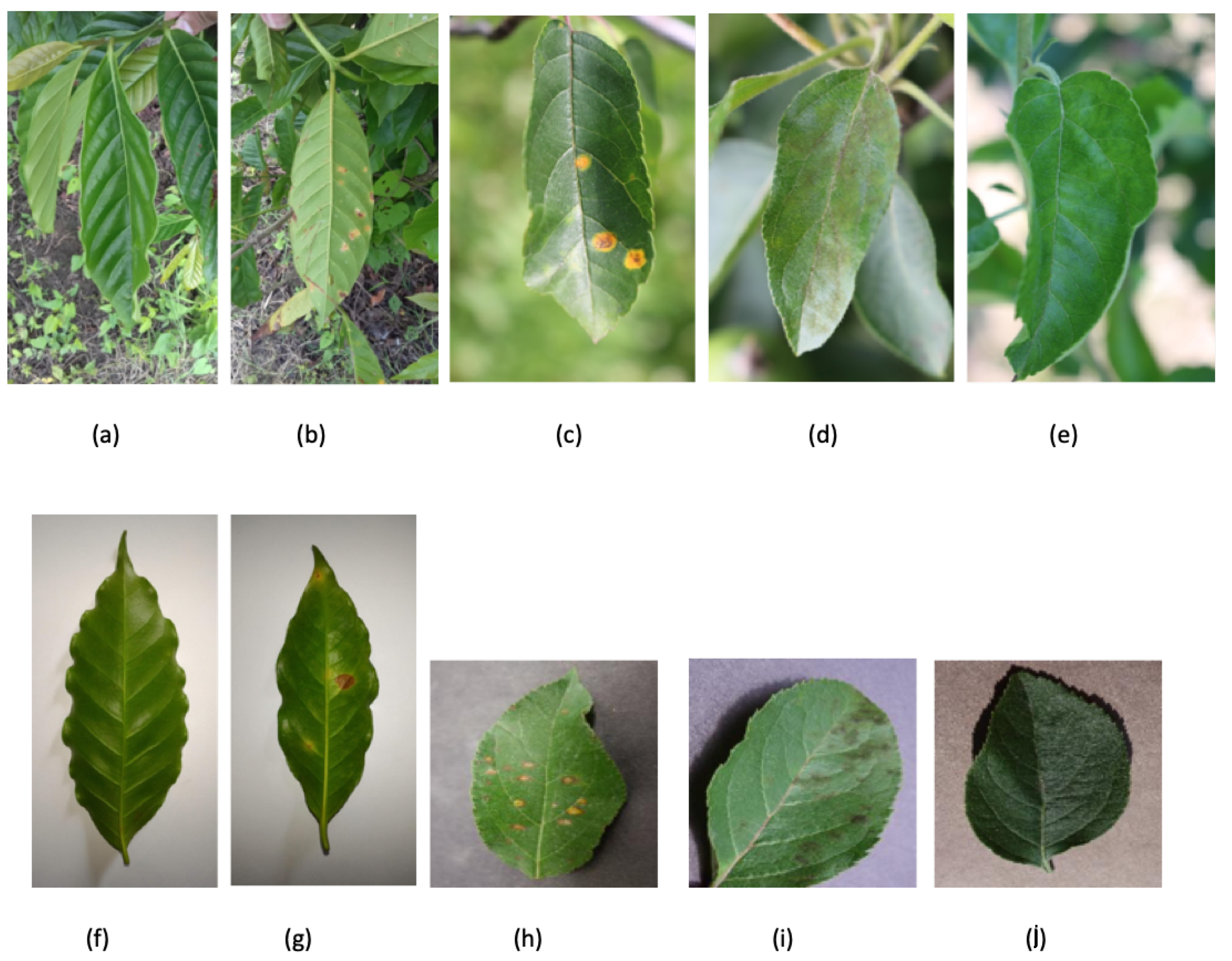
For the purpose of our study, only healthy and rust disorders were taken into consideration. Plant Pathology, as defined by authors, is a dataset that consists of 3651 high-quality (i.e., high-resolution) images of multiple apple foliar diseases captured in field conditions, and annotated into four classes: scab, cedar apple rust, multiple diseases and healthy. A subset of this dataset was made available to the Kaggle community for a Plant Pathology Challenge. In our work, only healthy, cedar rust and scab leaves were examined. The PlantVillage dataset comprises healthy and diseased leaf images into 38 labels (54,306 images, 26 diseases, 14 crop species), portrayed only on the ventral side of the leaf, on a homogeneous background. From this dataset, we selected only the apple leaves affected by three main biotic stresses: cedar rust, scab and healthy leaves. For each dataset, we balanced the classes. Table 2 summarizes the dataset in its entirety, reporting the cultivation, the conditions in which it was collected, the disease and the number of images for each of them. Figure 1 shows samples of images in each dataset.
2.2. Experimental Approach
We adopted five notable convolutional neural networks architectures for the investigation of our study, including VGG16 [27], ResNet50 [28], InceptionV2 [9], MobileNetV2 [29] and EfficientNetB0 [30]. We considered these architectures not only because their effectiveness was proven in previous works [21,31,32,33] that deal pretty well with plant disease classification, but also because they portray a representative sample of the modern architectures studied today for the solution of the problem under examination.
Since the first moment in which convolutional neural networks were theorized in the literature, they have undergone a progressive evolution aimed at: (1) improving performance; (2) solving technical problems such as vanishing gradient problem, overfitting, (3) improving the use of resources. The VGG network [27] follows the archetypal pattern of classic convolutional networks. It was designed to achieve high accuracy. Indeed, thanks to its simplicity, and the use of deep layers with small filters, it scored first place in the image localization task and second place in the image classification task in the Image Net Large-Scale Visual Recognition Challenge (ILSVRC). After its introduction in research, more efforts were concentrated on the development of architectures that suffered less from the vanishing gradient problem and overfitting. He et al. [28] ideated the concept of residual learning, developing a residual neural network called ResNet50. Furthermore, to cope with the need to integrate intelligent models into devices with limited resources, more branched and performing networks have been built in real-time mode, such as InceptionV2 [9], as well as lighter networks, structured for an efficient use of computational resources, both in terms of memory and time, such as MobileNet [29] and EfficientNet [30]. The reader is referred to the respective papers for a detailed description of each of them. From the brief historical excursus, it is inferred that the comparison of these architectures provides a baseline that can be used in future studies on the subject.
Although CNNs are shown to achieve significant results on image classification task, there are problems with implementation and use. Among these, neural networks require a large number of samples for proper training. Thus, designing and training a CNN from scratch is not considered an ideal solution when dealing with a small dataset. In light of this challenge, the concept of transfer learning is adopted.
2.3. Transfer Learning
Transfer learning is a strategy widely used in deep learning to yield reasonable results despite a relative lack of data. It consists of taking features learned on one problem and leveraging them on a new similar problem [34]. In other words, it reuses the weights of a pretrained model, to initialize and estimate the weights in a new model designed for the target task.
2.4. Data Augmentation
Data augmentation is a method used to mitigate overfitting in computer vision. It is a data enrichment method in which new training samples are generated from the training dataset by applying a series of random transformations. At the state of the art, there are several tools that introduce more variability into the dataset. The standard techniques include rotation, shearing, zooming, cropping, flipping and color variation. In this work, we focused on standard methods in order to improve the performance and the generalizability of the model.
2.5. Experimental Setup
The experimental framework written in Python language exploits the Keras deep learning 2.4.3 library based on Tensorflow 2.2.1 environment, executed on a server equipped with a 3.000 GHz Intel(R) Xeon(R) Gold. To carry out the study, we divided the dataset into training, validation, and test datasets with a ratio of 6:2:2, respectively. To preserve the percentage of samples for each class, the dataset was split using the ShuffleSplit strategy provided by the scikit-learn 0.23.2 library. Before training, we preprocessed the data to meet the requirements of CNN networks. All images were resized to 224 × 224 × 3, reshaped into the shape the networks expect and scaled so that all values were in the [0, 1] interval. A data augmentation technique was applied in real time during the training phase with a probabilistic execution of horizontal and vertical mirroring, rotation, and color variation. The CNN networks received slightly different images for each batch, and the analysis allowed them to adjust the network’s weights until the network learned the most relevant features for the given problem [7]. The transfer learning as feature extraction was performed by adapting CNN networks trained using the ImageNet dataset [35], which consists of images from a large variety of objects (1000 categories). During this step, the top layers were frozen to prevent their weights from being updated during training. Thus, with this configuration, the features that were previously learned from the convolutional base were not lost. The hyper-parameters configurations used are presented in Table 3, where loss function was set to binary entropy for binary classification (RoCoLe, BRACOL datasets), while cross entropy was employed for multi-label classification (Plant Village, Plant Pathology datasets). We monitored the model’s validation loss to reduce the learning rate when it stopped improving. This strategy allowed us to get out of local minima during training, a phenomenon known as Plateau [36]. The learning rate decreased when the validation loss stopped improving for 4 epochs, dividing it by 10. Finally, the states (set of weights) in which the networks presented the lowest loss value for the validation set were saved. The saved models are evaluated with the test dataset and the results are computed in terms of Accuracy, Precision, Recall, F1-score.
2.6. Metrics
Given the nature of our work, which distinguishes healthy leaves from diseased leaves affected by different pathogens, we evaluated the impact that occurred in the classification of plant diseases using datasets captured under different conditions in terms of classification accuracy metrics, including Accuracy, Precision, Recall and F1 score. In addition, the Confusion Matrix was computed to better understand how the classifiers performed with respect to the target classes in the dataset. To interpret the reasons for misclassifications, a visual explanation from the deep networks with attention maps was also provided by applying the Gradient-Weighted Class Activation Mapping (Grad-CAM) technique.
2.6.1. Classification Accuracy Metrics
In the description of these evaluation metrics, we used the following definitions: False Positives (FP): diseased leaves that were misclassified as healthy; False Negatives (FN): heathy leaves that were misclassified as diseased; True Positive (TP): diseased leaves that were correctly classified as diseased; True Negative (TN): healthy leaves that were correctly classified as healthy. We measured the following metrics:
- Accuracy is defined as ;
- Precision is defined as ;
- Recall is defined as ;
- F1 score is defined as ;
- The confusion matrix is a table that displays and compares actual values with the model’s predicted values. It provides detailed information on how a classifier performed on a dataset. Table 4 reports a template of the confusion matrix used for the binary classification.
2.6.2. Interpreting the Classification through Feature Visualization
Initially, deep learning was regarded as a “black box” [9] because the features that are learned by CNN-based models are difficult to represent in a human-readable form. In recent years, the contents of the black box have been unveiled thanks to the recent growth of deep learning research. Researchers developed different techniques capable of extracting the CNN calculation process in a human-interpretable form, such as via visualization. A detailed analysis of these techniques applied to plant classification is provided in [37]. In our work, the Gradient-Weighted Class Activation Mapping (Grad-CAM) technique [38] was applied to reveal the features and regions within the image which have been important in the classification. As described by the authors [38], Grad-CAM uses the gradient information flowing into the last convolutional layer of the CNN to assign importance values to each neuron for a particular region of interest. Although this technique is fairly general, in that it can be used to explain activations in any layer of a deep network, in our study, we focus on explaining output layer decisions only, in order to better understand the correct classification and misclassifications.
3. Results
This section reports the results obtained to assess how much the representativeness of the datasets affects the classification of diseased leaves.
3.1. Classification Accuracy Metrics and Convergence Speed Comparisons
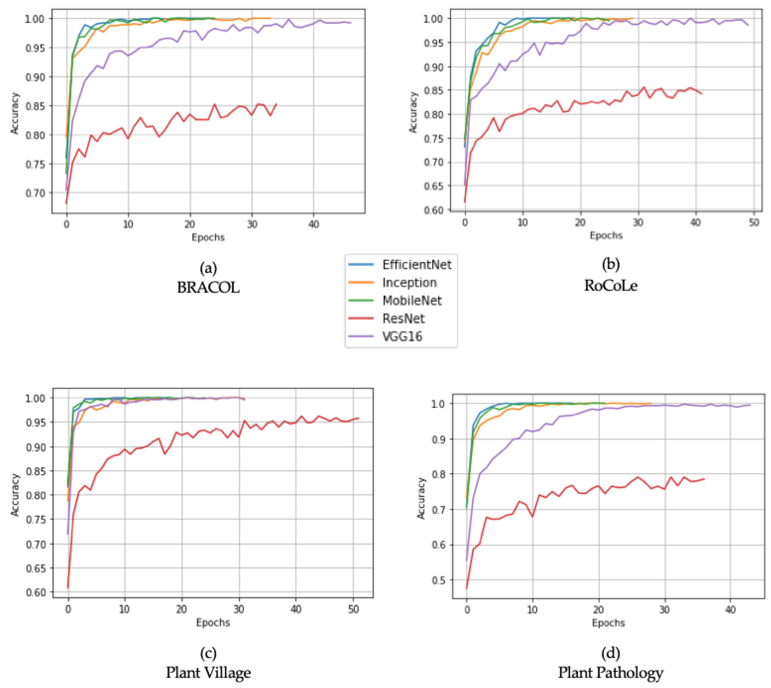
Table 5 lists the test accuracy obtained with deep neural networks as feature extractors for each dataset, while Figure 2 plots the accuracy curve during the training phase. Through analysis of the results, it can be seen that all classifiers scored better in the laboratory datasets than the field datasets, both for binary classification and for multiclass classification. This behavior can be attributed to the different levels of variability present in field images, where real-world factors increase the complexity of the problem, e.g., the background and different angles of the light beam. MobileNetV2 identified the salient patterns for classification in all four datasets, followed by EfficientNetB0, InceptionV2, VGG16, and ResNet50. In detail, MobileNetV2 and EfficientNetB0 achieved very close performance for laboratory datasets, and outperformed the other architectures. MobileNetV2 scored 87.02% (RoCoLe), 87.31% (Plant Pathology), while EfficientNetB0 scored 82.90% (RoCoLE) and 82.57% (Plant Pathology). VGG16 achieved high results for the BRACOL (96.54%) and Plant Village (97.84%) datasets, but had a marked decline in accuracy for the field datasets, 79.83% for RoCoLe, and 70.11% for Plant Pathology. Lower results across all datasets were recorded by ResNet50. In terms of convergence speed, as expected considering the nature of the architectures, the EfficientNetB0, MobileNetV2 and InceptionV2 networks converge faster than the VGG16 and ResNet50 networks. The first models converge after 20 epochs, while the last two models converge after 40 epochs (see Figure 2).
Table 6 graphically shows the precision, recall and F1 score for each model. Evaluating the models using these metrics confirms the rankings identified with accuracy, in which MobileNetV2 performed best, followed by EfficientNetB0, InceptionV2, VGG16 and ResNet50. In this case, MobileNetV2 is more accurate than EfficientNetB0. In terms of recall, MobileNetV2 obtained a high rate for field datasets 87.02% (RoCoLe) and 87.31% (Plant Pathology), while EfficientNetB0 achieved 82.59% (RoCoLe) and 82.79% (Plant Pathology), respectively. The MobileNetV2, EfficientNetB0, InceptionV2, VGG16 architectures are all precise and sensitive. Indeed, the F1 score metric that carries out a harmonic average of the two metrics remains raised. On the contrary, ResNet50 is highlighted, as its precision and recall are inversely proportional. In fact, the model is more precise and less sensitive. This inference is more notable in field datasets. Graphs of training accuracy and loss are released as supplemental material.
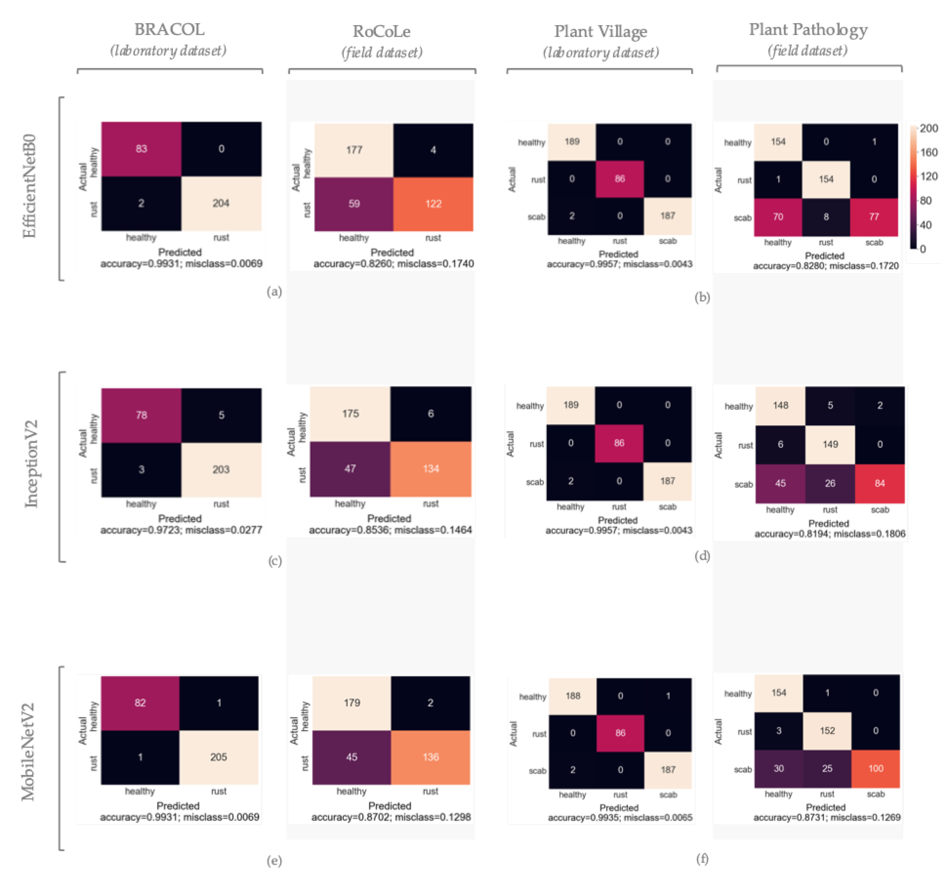
By analyzing the confusion matrix of the networks that achieved high results, it is possible to perform a more detailed observation of the errors made by the classifiers (see Figure 3). For the RoCoLe dataset, all three classifiers swapped rust-affected leaves for healthy leaves. For the respective laboratory dataset named BRACOL, the InceptionV2 model made multiple mistakes in labeling healthy leaves as diseased. In the laboratory datasets for the multiclass classification, it is observed that errors are more committed in classifying the leaves affected by scab as healthy. The same trend is present in the field dataset. The classifiers find it very difficult to distinguish the scab class from the healthy class, as the symptoms of the disease are mild and superficial, so much so that they are not clearly visible in uncontrolled environmental conditions. By observing the incorrectly classified photographs with the naked eye, it is inferred that these symptoms are more evident, marked and distinguishable in laboratory photographs (see Figure 1d,e).
3.2. Interpreting the Classification through Feature Visualization
The Gradient-Weighted Class Activation Mapping (Grad-CAM) technique [38] was applied to reveal the features and regions within the image which were important in the classification of the leaves. Indeed, its use on the misclassified images enabled us to understand the reason why the CNN made an error, and its application to the correct classifications highlighted which regions of the image led to the individuation of the class.
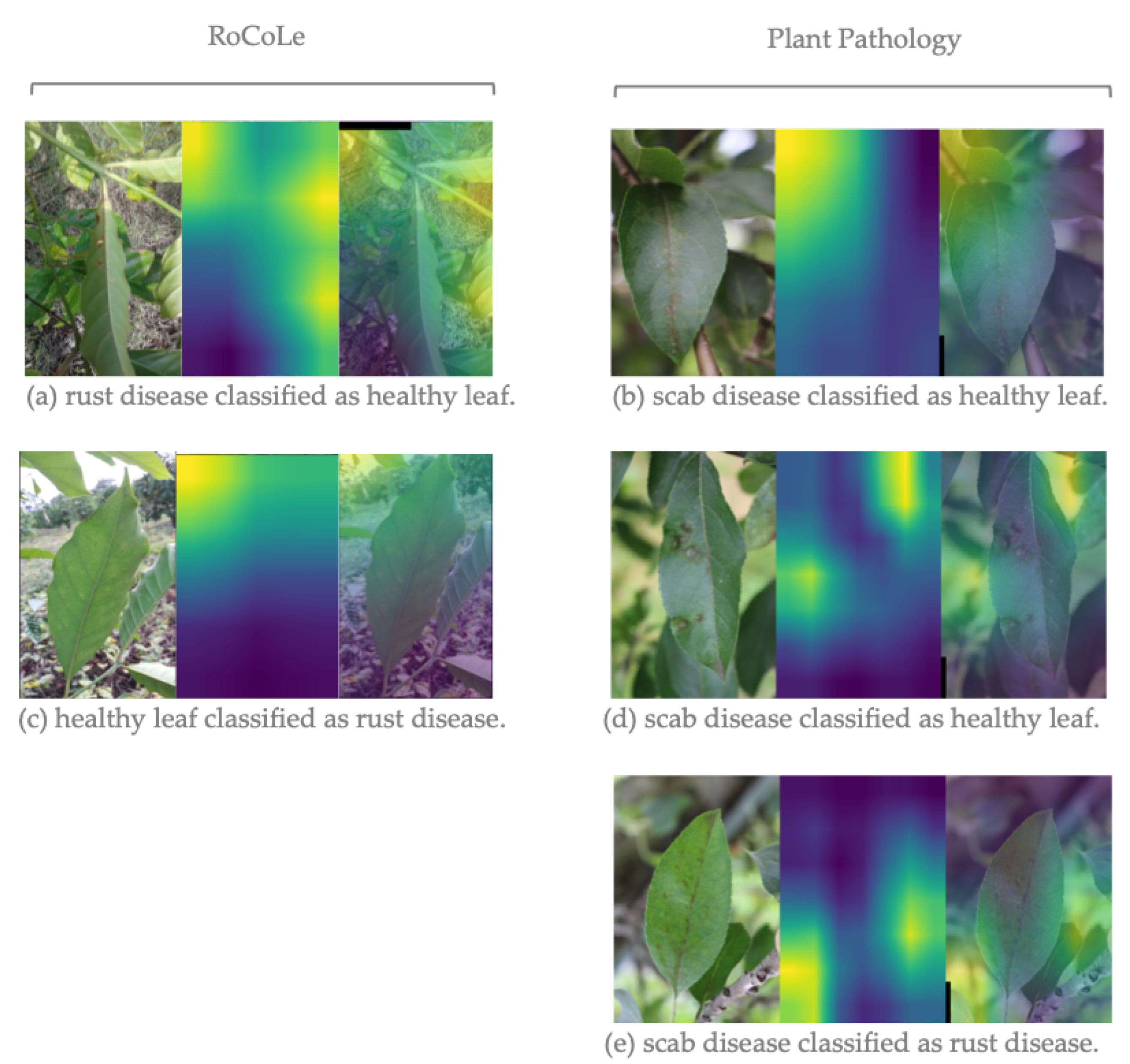
The investigation was conducted for the three models that performed best, i.e., MobileNetV2, InceptionV2, and EfficientB0. Figure 4 shows some examples of misclassification common to all three models for the field dataset. For each picture from left to right, we can see the original image, the generated heatmaps of class activation of the last convolution layer and the overlap of the two images. The first column shows the errors for the RoCoLe dataset. The leaf (a) affected by rust was classified as healthy, while the healthy leaf (b) was classified as diseased. In both cases, the network was unable to identify the leaf in the foreground, and the features that influenced the classification belonged to the leaves in the background. However, in image (a) the foreground leaf is completely out of focus. This distortion may have introduced a bias into the process and caused the classifier to analyze the elements in the background. The second column shows the errors for the Plant Pathology dataset. The scab class (b),(d) was classified as the healthy class. Note that the leaf in the (d) picture is partially focused, while the lesion is completely blurred. Similar to (a) image, the network may have been misled due to the noise in the photo. In photograph (d), the model gave more weight to the light-colored patches in the background, leading to a classification error. The same trend occurred in image (e), in which scab disease was classified as rust disease.
Alongside the investigation of the features through the Grad-Cam technique, we analyzed the groups of incorrect classifications on the RoCoLe and Plant Pathology field datasets, and outlined the factors that affected the results, reported below by adopting the categorization carried out by [16]:
3.3. Extrinsic Factors
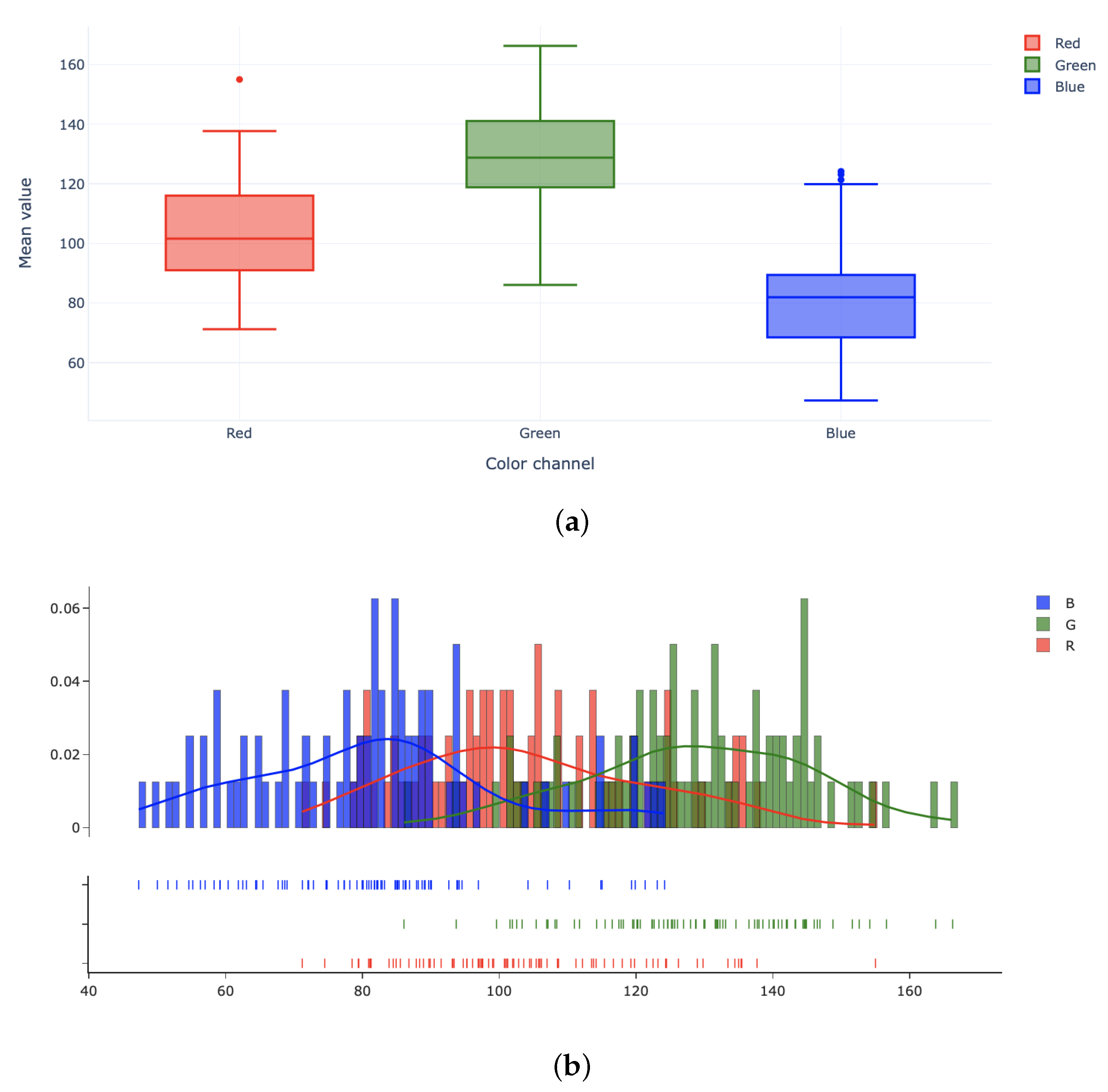
The complexity of the background, the lighting of the environment, the focus of the device, the location and the inclination of the leaf in the frame influence the classification of the images. The greatest difficulties are encountered when the background has a significant amount of green. Indeed, as shown by the Figure 5 the distribution of the green channel is the most pronounced, followed by red and blue. In particular, the distribution of the red color shows a slight rightward skew (positive skew), and a large variation in the average values of red across the images. The lighting of the image is a disturbing factor at certain angles of view, especially when it is directed at the leaf. Focus compromises analysis in photos where the leaf is completely or partially out of focus on a sharp background. Furthermore, the classifier tends to make mistakes when the leaf is not well centered in the frame, when it is very far from the capture point or when it is partially occluded by another leaf.
3.4. Intrinsic Factors
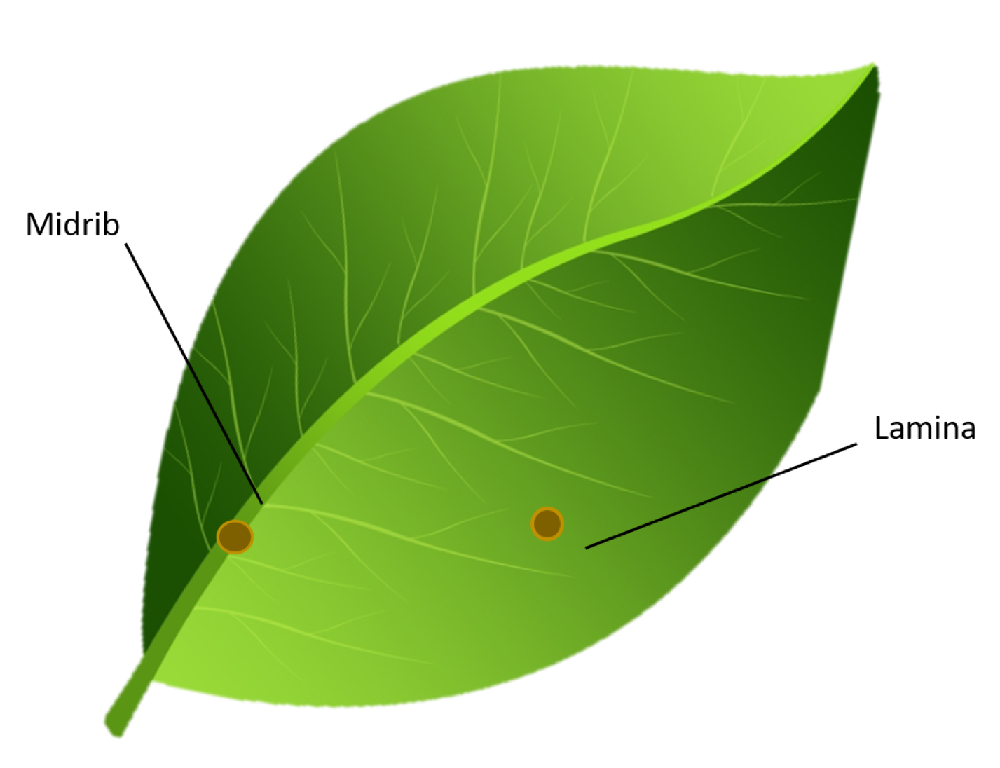
There are leaves in the datasets where the disease is more pronounced and marked than others. The largest misclassifications occurred with mild or small symptoms, and with dissolved contours. The location of the symptom appears difficult to identify if placed along the midrib or lamina, as shown in Figure 6. Further, we observed that the size and shape of the leaf also affect the classification process. Indeed, considerable difficulties arise when the leaf is small, when it is folded in on itself, when it has leaf holes or when it is broken.
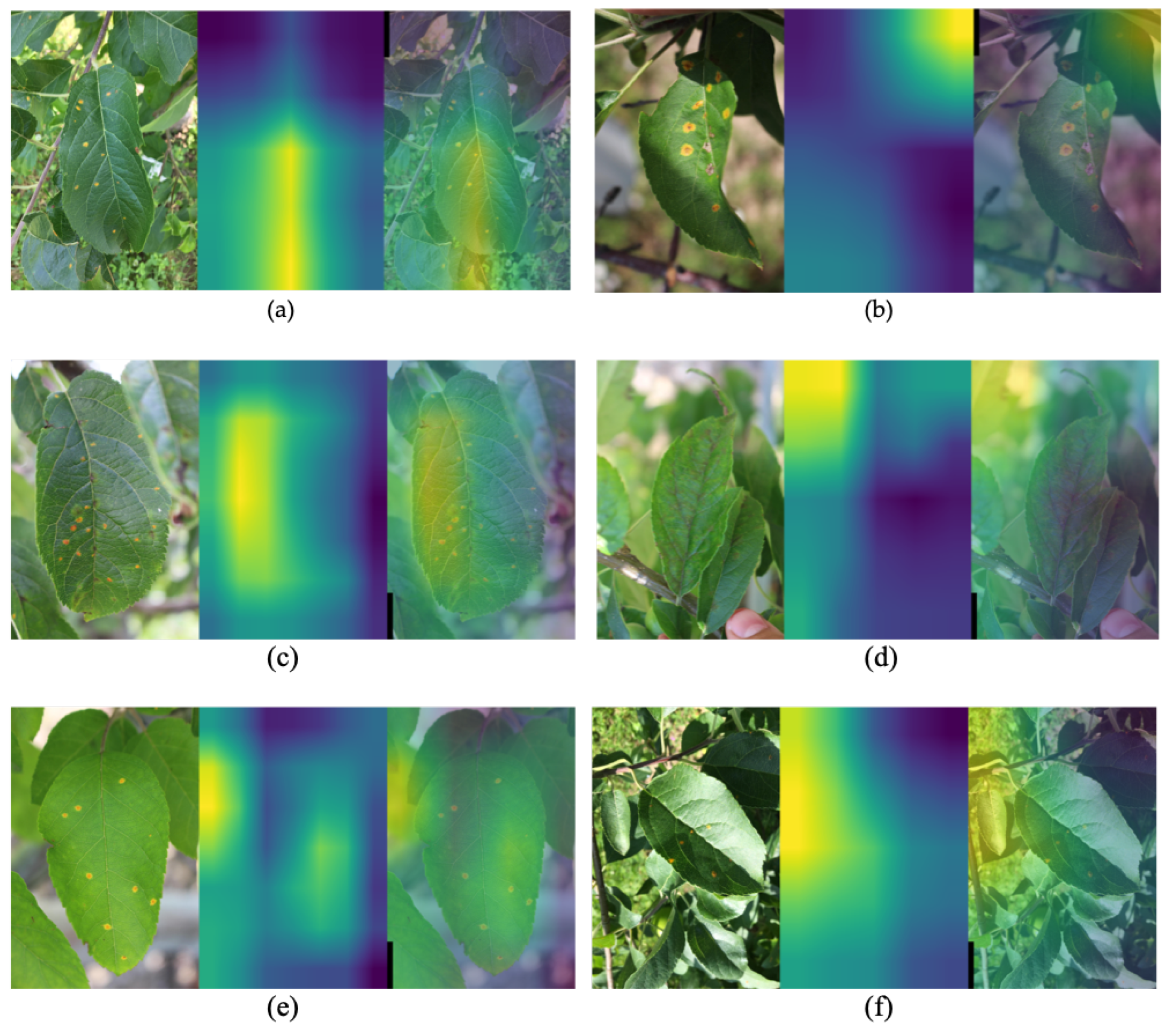
A detailed inspection of the correctly identified images by MobileNetV2, EfficientB0, and InceptionV2, was further conducted alongside the misclassifications. Figure 7 and Figure 8 show some representative examples of the Plant Pathology and Plant Village datasets, respectively. From this investigation, we can observe how the classifier behaves in detecting the health status of the leaf in different environmental conditions. In the laboratory dataset, the convolutional neural network always focuses on the leaf and its symptom as a point of interest (see Figure 8). The correct analysis is certainly facilitated by the little extrinsic variability present due to a homogeneous background that increases the contrast of the edges, and well-configured lighting conditions. However, the same trend is not found for the leaves retracted on the plant. The first column of Figure 7 depicts the images in which the damaged leaf parts contributed most to the distinction of classes. On the contrary, in the second column, we observe a similar trend to the wrong classifications. Although the leaf was correctly classified, the features learned from the model do not belong to the leaf in the foreground, but to the leaves in the background. From the (b), (d), and (f) images of Figure 7, we can observe the regions where the activations occurred (regions in yellow), which belong to the underlying leaves affected by the same disease as the leaf in relief.
3.5. Investigating Preprocessing Impact
Based on the results obtained (see Section 3) and feature inspection, an additional experiment was conducted to investigate the impact of preprocessing in the field datasets. Specifically, the RoCoLe dataset was examined. For each image, based on the bounding box and its mask, the background was removed. Therefore, the image was cropped and resized to meet the input size requirement illustrated in Section 2.5. The results are presented in Table 7. The scores obtained reveal a negative impact. Removing the background lowered the performance of the top three convolutional networks from an average of 85% accuracy to an average of 72% accuracy. In theory, this practice should not deteriorate the classification performance, but it is assumed that it should produce an improvement. Therefore, we infer that in this case study, models exploit background features in the decision-making phase. In light of these observations, we investigated from the set of misclassifications whether the detected errors were committed on the same images to which preprocessing was not applied. We found that EfficientNetB0 committed the same errors on 50% of the original images, MobileNetV2 38%, and InceptionV2 36%, respectively. The models had more difficulty in discriminating the rust class.
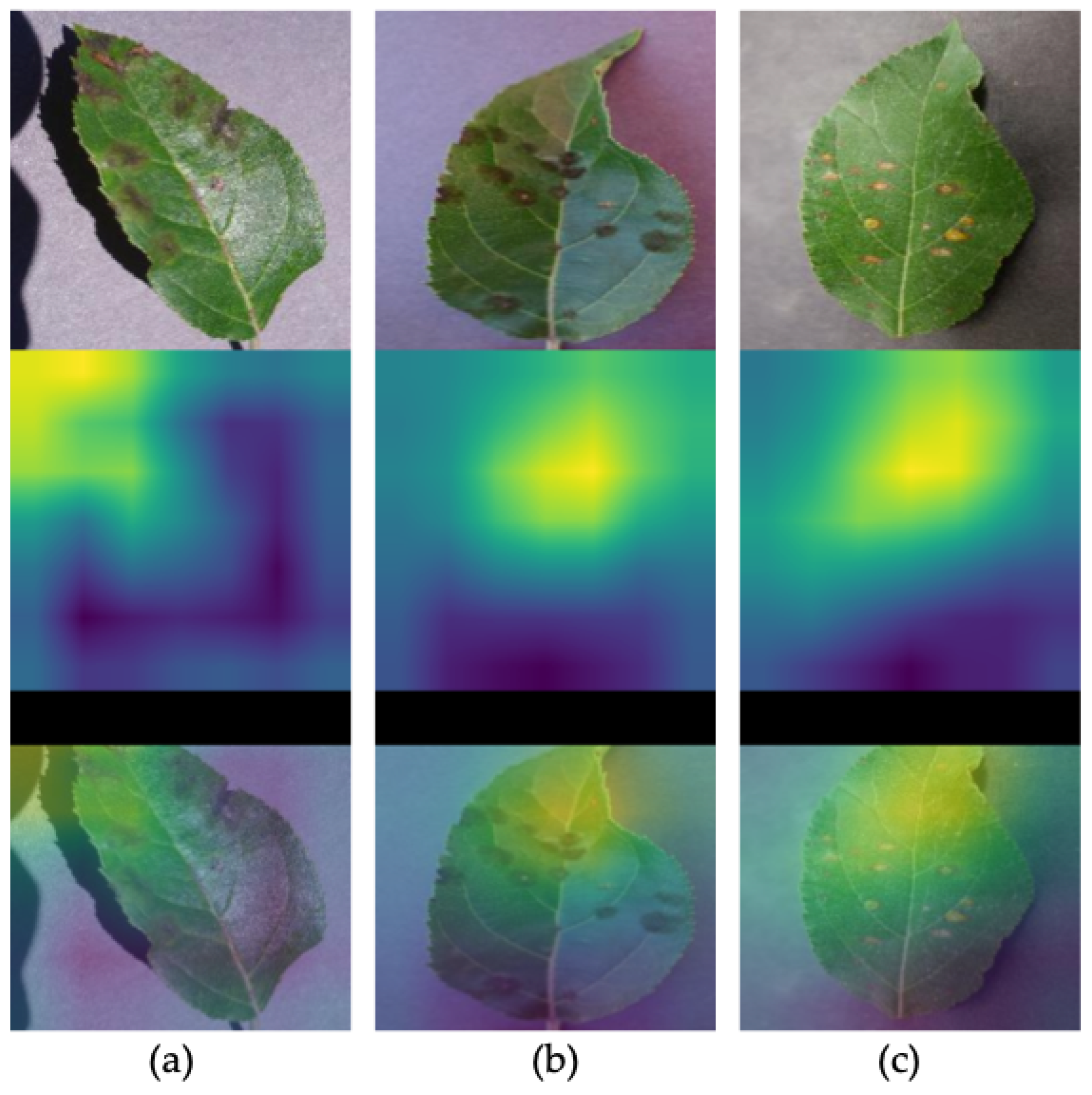
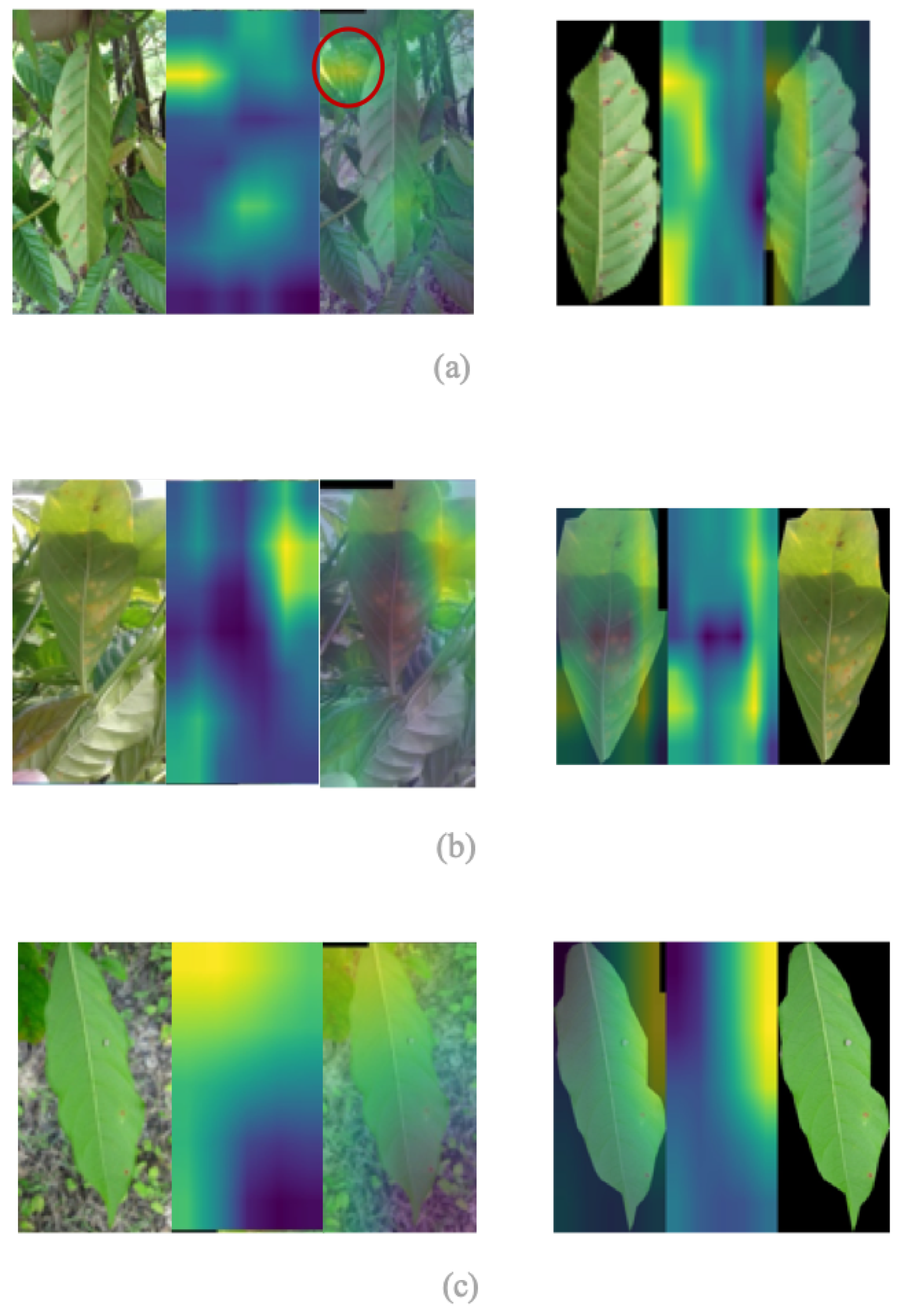
Given O the set of misclassifications of the original images to which preprocessing was not applied and given P the set of misclassifications to which preprocessing was applied, for each network , we applied the Grad-Cam technique to the set in order to investigate why the original correctly classified images were misclassified following the application of background removal. Representative samples of the misclassifications are shown in Figure 9. The correct classification obtained in the first case study is shown on the left; on the right is the same image with the background removed, but classified incorrectly.
The analysis shows that the classification had a negative impact for several reasons. As Figure 9 shows, in most of the correctly classified images, the background played a decision-making role in the final prediction. The leaf in the background (Figure 9a), circled in red, strongly activated the network. Indeed, following the isolation of the region of interest, the classifier was unable to identify the disease. Similarly, it is observed that errors occurred under suboptimal illumination conditions (Figure 9b), i.e., strong contrasts due to overexposure or underexposure of the image. Finally, it was observed as occurring in the analysis without preprocessing. The factors that hindered class discrimination were small size (Figure 9c) and dissolved symptom contours.
4. Discussion
The proposed study was designed to evaluate factors limiting the classification of plant diseases using datasets acquired under different conditions, e.g., laboratory, and field.
In recent years a number of researchers have provided different proof of concept regarding the use of deep learning for the classification of leaf diseases. Due to the limited availability of data, several experiments have been conducted on similar and laboratory-built datasets, the use of which has led the models to achieve high performance in terms of accuracy (see Table 8).
In this study, we conducted an evaluation on the datasets’ representativeness, analyzing the problem both as a binary classification and as a multiclass classification.
The results obtained are not directly comparable with other studies in the literature, as different datasets, plant diseases and parameters were considered. However, there is some coherence concerning the results achieved with those of similar works. For example, the research in [31] compared VGG and AlexNetOWTBn architectures to estimate 58 plant diseases. The dataset employed contained images captured in both experimental setups, i.e., laboratory and field conditions. The authors noted that success rates were significantly lower when the model was trained solely on laboratory-condition images. Similarly, the study in [39] classified six biotic stresses captured in field conditions, comparing different CNN architectures, including VGG16, ResNet50 and Inception. The experiments performed by the authors achieved overall accuracy of 76.20% (VGG16), 81.70% (ResNet50), and 85% (Inception) and in our experiments, we achieved accuracy of 79.83% (VGG16), 67.40% (ResNet50), and 85.36% (Inception), respectively. This indicates the need to understand the degree of transferability of the models trained on the laboratory datasets in a real-world scenario, quantifying the factors limiting the classification.
Even if our investigation involved four datasets, due to their limited availability in the literature, the results obtained provide a useful reference line for the construction of more robust models and comprehensive datasets.
Inspection of the confusion matrices and activation maps of the last layers revealed several aspects. In the laboratory dataset, the healthy class is well identified. Conversely, some errors occur in the field dataset. Likewise, classifiers detect rust disease caught in the lab and slightly less so in the field. This behavior reported in the binary classification becomes more pronounced in the multiclass classification, where a high number of leaves affected by scab were classified as healthy and affected by rust.
To this end, in addition to providing a GAP performance among recent convolutional architectures to predict the same crop disease in different environmental conditions, we quantified the impact of extrinsic and intrinsic factors.
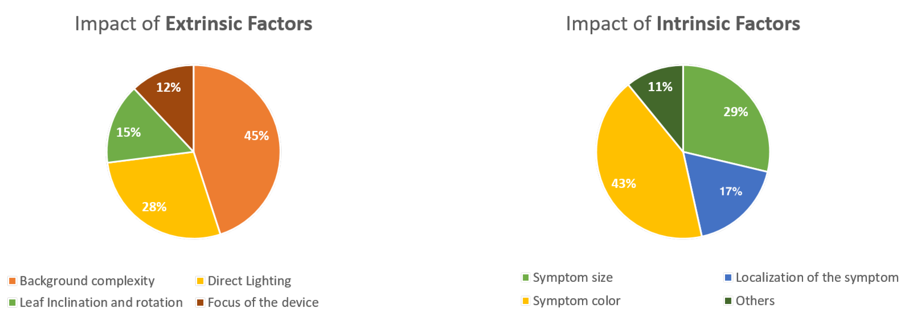
Among the factors enunciated in [16], in our study, we have identified the most significant: background complexity (45%), direct lighting (28%), leaf inclination and rotation (15%), focus of the device (12%), symptom color (43%), symptom size (29%) and location of the sympthoms (17%) (see Figure 10).
When the image contains a background with a high distribution of green color, the classifier is unable to focus the leaf in the foreground, but tends to analyze the elements near the leaf in question and at the edges of the image. This behavior is found especially when the symptom is very mild, clear, dissolute, small and localized on the midrib and/or lamina (see Figure 6). The markedness of the symptom is a very important factor for the management of parasitic adversities. If any classifier does not encounter major obstacles in identifying small lesions under controlled conditions, the difficulties arise when they are photographed in the field. However, the automatic recognition of the disease in the early stages of onset is an essential tool to act promptly and stem possible damage. For farmers, this tool is particularly useful in the early stages, when the symptom is not yet well defined and is minor, and subtle injuries can lead to decision errors. It must be borne in mind that when the symptom is in a more advanced and defined phase, farmers are able to recognize it with the naked eye; therefore, the usefulness of automatic recognition systems is attenuated. These tools remain equally essential in rural areas in which access to agronomic advice is difficult.
Finally, by analyzing the correct clusters, it is observed that the features and parts of the image that lead the network to its final decision do not always belong to the object under examination. Several times, the classifier uses elements belonging to the background, e.g., other leaves that have the same/different symptoms as the foreground leaf. This behavior occurs more when the leaf is distant from the capture device, and the background occupies a significant amount in the frame. In light of this, the impact of the background was investigated. We have observed that the removal of the background degrades the results when the dataset is collected under realistic conditions. This is due to the fact that the prediction of the original images without preprocessing is highly dependent on the presence of the background, which—in its absence—results in a lower accuracy rate.
5. Conclusions
The classification of plant diseases from leaf images has been addressed via deep learning in recent years. The literature has focused more on the exploration of laboratory datasets, with less investigation of the transferability of models in practice. Generalizing an algorithm—that is, achieving performance of similar classifications—is possible only when the training data are similar to the new data to which you want to apply the model. The main contribution of this study was the evaluation of the factors limiting the classification by analyzing the same leaf disease in different capture conditions, controlled and not, quantitatively investigating the categorization of the extrinsic and intrinsic factors stated in [20]. To this end, four state-of-the-art datasets were used, to which class balancing was applied, and binary and multiclass classification were studied. The scores obtained show a drastic drop in performance from the laboratory dataset to the field dataset. In the worst case, the accuracy dropped from 92.67% to 54.41%. Among the most relevant extrinsic factors were the complexity of the background, while the most relevant intrinsic factors included the size and color of the symptom.
The results are strongly influenced and linked to the dataset representativeness, but also to the ability of the model to learn the salient features when the analysis is carried out on small objects of interest. The region focused by the CNN does not always belong to the lesion of the leaf in the foreground. Sometimes, the classifier tends to focus on the background elements. The removal of the background had a serious impact on the results, showing that the models achieve high performance by exploiting the elements of the background. Indeed, the algorithm errs when the symptom is in the initial stage of appearance, small in size, not very pronounced, and with clear and dissolved contours.
In conclusion, in this study, we have provided a baseline performance of the most recent convolutional architectures, quantifying the factors limiting the resolution of the problem to be taken into consideration both for the construction of algorithms and for the construction of new datasets. These limitations still prevent this technology from being used in practice. The latter can be overcome by building more consistent datasets [23], and more complex models that integrate a leaf spot attention mechanism to increase the discriminatory power and extract information features from the leaf blade.
Our results can be easily reproduced using our open-source toolbox, called LeafBox (https://leafbox.francescamalloci.com/, https://github.com/mallociFrancesca/leaf-disease-toolbox, accessed on 17 October 2022), written in python as a modular and reusable tool. This allows us to combine different analysis techniques in order to simplify the analysis processes and facilitate the reproducibility and sharing of experimental results with the scientific community.
Supplementary Materials
The following supporting information can be downloaded at: https://0-www-mdpi-com.brum.beds.ac.uk/article/10.3390/agronomy12102359/s1.
Author Contributions
All authors equally contributed to this research. All authors have read and agreed to the published version of the manuscript.
Funding
This research received no external funding.
Data Availability Statement
The source code is available at https://leafbox.francescamalloci.com/, https://github.com/mallociFrancesca/leaf-disease-toolbox, accessed on 17 October 2022.
Acknowledgments
We would like to thank the reviewers whose valuable feedback, suggestions and comments significantly increased the overall quality of this study.
Conflicts of Interest
The authors declare no conflict of interest.
References
- Asongu, S.A.; Le Roux, S.; Biekpe, N. Enhancing ICT for environmental sustainability in sub-Saharan Africa. Technol. Forecast. Soc. Chang. 2018, 127, 209–216. [Google Scholar] [CrossRef]
- Newbery, F.; Qi, A.; Fitt, B.D. Modelling impacts of climate change on arable crop diseases: Progress, challenges and applications. Curr. Opin. Plant Biol. 2016, 32, 101–109. [Google Scholar] [CrossRef] [PubMed]
- Fenu, G.; Malloci, F.M. Forecasting Plant and Crop Disease: An Explorative Study on Current Algorithms. Big Data Cogn. Comput. 2021, 5, 2. [Google Scholar] [CrossRef]
- Malloci, F.M.; Penadés, L.P.; Boratto, L.; Fenu, G. A Text Mining Approach to Extract and Rank Innovation Insights from Research Projects. In Proceedings of the International Conference on Web Information Systems Engineering, Amsterdam, The Netherlands, 20–24 October 2020; Springer: Berlin/Heidelberg, Germany, 2020; pp. 143–154. [Google Scholar]
- Fenu, G.; Malloci, F.M. Artificial Intelligence Technique in Crop Disease Forecasting: A Case Study on Potato Late Blight Prediction. In Proceedings of the International Conference on Intelligent Decision Technologies, Split, Croatia, 17–19 June 2020; Springer: Berlin/Heidelberg, Germany, 2020; pp. 79–89. [Google Scholar] [CrossRef]
- Fenu, G.; Malloci, F.M. An Application of Machine Learning Technique in Forecasting Crop Disease. In Proceedings of the 2019 3rd International Conference on Big Data Research, France, Paris, 20–22 November 2019; pp. 76–82. [Google Scholar] [CrossRef]
- Fenu, G.; Malloci, F.M. Using Multi-Output Learning to Diagnose Plant Disease and Stress Severity. Complexity 2021, 2021, 18. [Google Scholar] [CrossRef]
- Brahimi, M.; Boukhalfa, K.; Moussaoui, A. Deep learning for tomato diseases: Classification and symptoms visualization. Appl. Artif. Intell. 2017, 31, 299–315. [Google Scholar] [CrossRef]
- Szegedy, C.; Liu, W.; Jia, Y.; Sermanet, P.; Reed, S.; Anguelov, D.; Erhan, D.; Vanhoucke, V.; Rabinovich, A. Going deeper with convolutions. In Proceedings of the 2015 IEEE Conference on Computer Vision and Pattern Recognition (CVPR), Boston, MA, USA, 7–12 June 2015. [Google Scholar] [CrossRef]
- Sladojevic, S.; Arsenovic, M.; Anderla, A.; Culibrk, D.; Stefanovic, D. Deep neural networks based recognition of plant diseases by leaf image classification. Comput. Intell. Neurosci. 2016, 2016, 3289801. [Google Scholar] [CrossRef]
- Barré, P.; Stöver, B.C.; Müller, K.F.; Steinhage, V. LeafNet: A computer vision system for automatic plant species identification. Ecol. Inform. 2017, 40, 50–56. [Google Scholar] [CrossRef]
- Shrivastava, V.K.; Pradhan, M.K.; Minz, S.; Thakur, M.P. Rice plant disease classification using transfer learning of deep convolution neural network. Int. Arch. Photogramm. Remote. Sens. Spat. Inf. Sci. 2019, 3, 631–635. [Google Scholar] [CrossRef]
- Liu, B.; Zhang, Y.; He, D.; Li, Y. Identification of apple leaf diseases based on deep convolutional neural networks. Symmetry 2017, 10, 11. [Google Scholar] [CrossRef]
- Lu, Y.; Yi, S.; Zeng, N.; Liu, Y.; Zhang, Y. Identification of rice diseases using deep convolutional neural networks. Neurocomputing 2017, 267, 378–384. [Google Scholar] [CrossRef]
- Too, E.C.; Yujian, L.; Njuki, S.; Yingchun, L. A comparative study of fine-tuning deep learning models for plant disease identification. Comput. Electron. Agric. 2019, 161, 272–279. [Google Scholar] [CrossRef]
- Barbedo, J.G.A. A review on the main challenges in automatic plant disease identification based on visible range images. Biosyst. Eng. 2016, 144, 52–60. [Google Scholar] [CrossRef]
- Priyadharshini, R.A.; Arivazhagan, S.; Arun, M.; Mirnalini, A. Maize leaf disease classification using deep convolutional neural networks. Neural Comput. Appl. 2019, 31, 8887–8895. [Google Scholar] [CrossRef]
- Ji, M.; Zhang, L.; Wu, Q. Automatic grape leaf diseases identification via UnitedModel based on multiple convolutional neural networks. Inf. Process. Agric. 2020, 7, 418–426. [Google Scholar] [CrossRef]
- Uğuz, S.; Uysal, N. Classification of olive leaf diseases using deep convolutional neural networks. Neural Comput. Appl. 2020, 33, 4133–4149. [Google Scholar] [CrossRef]
- Barbedo, J.G.A. Impact of dataset size and variety on the effectiveness of deep learning and transfer learning for plant disease classification. Comput. Electron. Agric. 2018, 153, 46–53. [Google Scholar] [CrossRef]
- Esgario, J.G.; Krohling, R.A.; Ventura, J.A. Deep learning for classification and severity estimation of coffee leaf biotic stress. Comput. Electron. Agric. 2020, 169, 105162. [Google Scholar] [CrossRef] [Green Version]
- Hughes, D.; Salathé, M. An open access repository of images on plant health to enable the development of mobile disease diagnostics. arXiv 2015, arXiv:1511.08060. [Google Scholar]
- Fenu, G.; Malloci, F.M. DiaMOS plant: A dataset for diagnosis and monitoring plant disease. Agronomy 2021, 11, 2107. [Google Scholar] [CrossRef]
- Parraga-Alava, J.; Cusme, K.; Loor, A.; Santander, E. RoCoLe: A robusta coffee leaf images dataset for evaluation of machine learning based methods in plant diseases recognition. Data Brief 2019, 25, 104414. [Google Scholar] [CrossRef]
- Krohling, R.; Esgario, J.; Ventura, J.A. BRACOL-A Brazilian Arabica Coffee Leaf images dataset to identification and quantification of coffee diseases and pests. Mendeley Data 2019, V1. [Google Scholar] [CrossRef]
- Thapa, R.; Zhang, K.; Snavely, N.; Belongie, S.; Khan, A. The Plant Pathology Challenge 2020 data set to classify foliar disease of apples. Appl. Plant Sci. 2020, 8, e11390. [Google Scholar] [CrossRef] [PubMed]
- Simonyan, K.; Zisserman, A. Very deep convolutional networks for large-scale image recognition. arXiv 2014, arXiv:1409.1556. [Google Scholar]
- He, K.; Zhang, X.; Ren, S.; Sun, J. Deep Residual Learning for Image Recognition. In Proceedings of the 2016 IEEE Conference on Computer Vision and Pattern Recognition (CVPR), Las Vegas, NV, USA, 27–30 June 2016. [Google Scholar] [CrossRef]
- Howard, A.G.; Zhu, M.; Chen, B.; Kalenichenko, D.; Wang, W.; Weyand, T.; Andreetto, M.; Adam, H. Mobilenets: Efficient convolutional neural networks for mobile vision applications. arXiv 2017, arXiv:1704.04861. [Google Scholar]
- Tan, M.; Le, Q.V. Efficientnet: Rethinking model scaling for convolutional neural networks. arXiv 2019, arXiv:1905.11946. [Google Scholar]
- Ferentinos, K.P. Deep learning models for plant disease detection and diagnosis. Comput. Electron. Agric. 2018, 145, 311–318. [Google Scholar] [CrossRef]
- Yan, Q.; Yang, B.; Wang, W.; Wang, B.; Chen, P.; Zhang, J. Apple Leaf Diseases Recognition Based on An Improved Convolutional Neural Network. Sensors 2020, 20, 3535. [Google Scholar] [CrossRef] [PubMed]
- Montalbo, F.J.P.; Hernandez, A.A. An Optimized Classification Model for Coffea Liberica Disease using Deep Convolutional Neural Networks. In Proceedings of the 2020 16th IEEE International Colloquium on Signal Processing & Its Applications (CSPA), Langkawi, Malaysia, 28–29 February 2020; pp. 213–218. [Google Scholar]
- Chollet, F. Deep Learning with Python; Manning Publications: New York, NY, USA, 2017. [Google Scholar]
- Deng, J.; Dong, W.; Socher, R.; Li, L.J.; Li, K.; Li, F.-F. ImageNet: A large-scale hierarchical image database. In Proceedings of the 2009 IEEE Conference on Computer Vision and Pattern Recognition, Miami, FL, USA, 20–25 June 2009. [Google Scholar] [CrossRef]
- Yoshida, Y.; Okada, M. Data-Dependence of Plateau Phenomenon in Learning with Neural Network—Statistical Mechanical Analysis. Adv. Neural Inf. Process. Syst. 2019, 32, 1722–1730. [Google Scholar] [CrossRef]
- Toda, Y.; Okura, F. How Convolutional Neural Networks Diagnose Plant Disease. Plant Phenomics 2019, 2019, 9237136. [Google Scholar] [CrossRef]
- Selvaraju, R.R.; Cogswell, M.; Das, A.; Vedantam, R.; Parikh, D.; Batra, D. Grad-cam: Visual explanations from deep networks via gradient-based localization. In Proceedings of the IEEE International Conference on Computer Vision, Venice, Italy, 22–29 October 2017; pp. 618–626. [Google Scholar]
- Ahmad, I.; Hamid, M.; Yousaf, S.; Shah, S.T.; Ahmad, M.O. Optimizing Pretrained Convolutional Neural Networks for Tomato Leaf Disease Detection. Complexity 2020, 2020, 8812019. [Google Scholar] [CrossRef]
- Atila, Ü.; Uçar, M.; Akyol, K.; Uçar, E. Plant leaf disease classification using EfficientNet deep learning model. Ecol. Inform. 2021, 61, 101182. [Google Scholar] [CrossRef]
- Chen, J.; Chen, J.; Zhang, D.; Sun, Y.; Nanehkaran, Y.A. Using deep transfer learning for image-based plant disease identification. Comput. Electron. Agric. 2020, 173, 105393. [Google Scholar] [CrossRef]
- Kamal, K.; Yin, Z.; Wu, M.; Wu, Z. Depthwise separable convolution architectures for plant disease classification. Comput. Electron. Agric. 2019, 165, 104948. [Google Scholar]
- Rangarajan, A.K.; Purushothaman, R.; Ramesh, A. Tomato crop disease classification using pre-trained deep learning algorithm. Procedia Comput. Sci. 2018, 133, 1040–1047. [Google Scholar] [CrossRef]
- Jasim, M.A.; Al-Tuwaijari, J.M. Plant leaf diseases detection and classification using image processing and deep learning techniques. In Proceedings of the 2020 IEEE International Conference on Computer Science and Software Engineering (CSASE), Duhok, Iraq, 16–18 April 2020; pp. 259–265. [Google Scholar]
- Wang, G.; Sun, Y.; Wang, J. Automatic image-based plant disease severity estimation using deep learning. Comput. Intell. Neurosci. 2017, 2017, 2917536. [Google Scholar] [CrossRef] [Green Version]
Figure 1.
Examples of leaves from the dataset employed. In the first line are reported the leaves collected in field, where (a,b) belong to ROCOLE dataset, and (c–e) belong to Plant Pathology dataset. From left to the right: (a) healthy coffee leaf; (b) rust coffee leaf; (c) cedar rust apple leaf; (d) scab apple leaf; (e) healthy apple leaf. In the second lines are reported the related leaves collected in a controlled environment, where (f,g) belong to BRACOL dataset, and (h–j) belong to Plant Village dataset. From left to the right: (f) healthy coffee leaf; (g) rust coffee leaf; (h) cedar rust leaf; (i) scab leaf; (j) healthy leaf.

Figure 2.
Comparison in terms of convergence speed and training accuracy. In the first column, we report laboratory datasets: (a) BRACOL, (c) Plant Village. In the second column, we report field datasets: (c) RoCoLe, (d) Plant Pathology.
Figure 2.
Comparison in terms of convergence speed and training accuracy. In the first column, we report laboratory datasets: (a) BRACOL, (c) Plant Village. In the second column, we report field datasets: (c) RoCoLe, (d) Plant Pathology.

Figure 3.
Confusion matrices obtained on test set. The first column contains the results for the binary classification of coffee leaves (BRACOL and RoCoLe datsets), while the second column contains the multiclass classification of apple leaves (Plant Village and Plant Pathology datasets). Each column on the left contains the results obtained via the laboratory dataset, and the right columns contain those obtained using the field dataset. The images (a,b) are the scores obtained by EfficientNetB0. The images (c,d) are the scores obtained by InceptionV2. The images (e,f) are the scores obtained by MobileNetV2.

Figure 4.
Misclassified pictures on field datasets obtained from MobileNetV2, InceptionV2, and EfficientB0. In each photo, from left to right, we see the original image, the generated heatmaps of the last convolution layer, and the overlap of the two images. The first column shows the errors for the RoCoLe dataset, whereas the second column depicts the error for the Plant Pathology dataset.

Figure 5.
Distribution of cluster channels (a) and (misclassification) (b).

Figure 6.
Major misclassifications occur when the leaf symptom is along the midrib or lamina.

Figure 7.
Damaged leaves (a,c,e) underlying leaves (b,d,f). Examples of images that were classified correctly belonging to Plant Pathology dataset. In each photo, from left to right, we see the original image, the generated heatmaps of the last convolution layer, and the overlap of the two images.
Figure 7.
Damaged leaves (a,c,e) underlying leaves (b,d,f). Examples of images that were classified correctly belonging to Plant Pathology dataset. In each photo, from left to right, we see the original image, the generated heatmaps of the last convolution layer, and the overlap of the two images.

Figure 8.
Examples of images that were classified correctly belonging to Plant Village dataset. In each photo, from left to right, we see the original image (a), the generated heatmaps of the last convolution layer (b), and the overlap of the two images (c).
Figure 8.
Examples of images that were classified correctly belonging to Plant Village dataset. In each photo, from left to right, we see the original image (a), the generated heatmaps of the last convolution layer (b), and the overlap of the two images (c).

Figure 9.
Representative examples of the correct classifications without preprocessing (left) and relative misclassifications with preprocessing (right). (a) is an example in which the classifier used parts of the background for the final decision. (b) shows the neural activations of the model under suboptimal lighting conditions. (c) highlights the behavior of the network in the presence of small symptoms.

Figure 10.
Factors influencing plant disease prediction classified as extrinsic and intrinsic factors.
Figure 10.
Factors influencing plant disease prediction classified as extrinsic and intrinsic factors.


Table 1.
The Table shows an overview of the datasets used, reporting the variables monitored and the total size, respectively. For a detailed description of the entire dataset, the reader is referred to the relevant manuscript.
Table 1.
The Table shows an overview of the datasets used, reporting the variables monitored and the total size, respectively. For a detailed description of the entire dataset, the reader is referred to the relevant manuscript.
| Dataset | Leaf Side | Variables | Number of Images |
|---|---|---|---|
| RoCoLe [24] | Adaxial and Abaxial | Healthy | 1560 |
| Red spider mite | |||
| Rust level 1 | |||
| Rust level 2 | |||
| Rust level 3 | |||
| Rust level 4 | |||
| BRACOL [25] | Abaxial | Healthy | 1747 |
| Miner | |||
| Rust | |||
| Phoma | |||
| Cercospora | |||
| Severity | |||
| Plant Pathology [26] | Adaxial | Healthy | 3651 |
| Cedar rust | |||
| Scab | |||
| Multiple diseases | |||
| Plant Village [22] | Adaxial | Healthy | 3172 |
| (only apple images) | Cedar rust | ||
| Scab |
Table 2.
Datasets details. The Table presents only the samples and the classes used to conducted the present case study as described in Section 2.2. For a detailed description of the entire dataset, the reader is referred to the relevant manuscript.
Table 2.
Datasets details. The Table presents only the samples and the classes used to conducted the present case study as described in Section 2.2. For a detailed description of the entire dataset, the reader is referred to the relevant manuscript.
| Dataset | Condition | Plant | Disease | Number of Images |
|---|---|---|---|---|
| RoCoLe [24] | Field | Coffee | Healthy | 602 |
| rust | 602 | |||
| BRACOL [25] | Laboratory | Coffee | Healthy | 684 |
| rust | 684 | |||
| Plant Pathology [26] | Field | Apple | Healthy | 516 |
| Cedar rust | 516 | |||
| Scab | 516 | |||
| Plant Village [22] | Laboratory | Apple | Healthy | 630 |
| Cedar rust | 630 | |||
| Scab | 630 |
Table 3.
CNN training hyper-parameters.
| Parameter | Value |
|---|---|
| Optimizer | RMSprop |
| Loss function | Binary-Entropy, Cross-Entropy |
| Learning rate | 2 × 10⁻⁵ |
| Momentum | 0.9 |
Table 4.
Confusion Matrix.
| Predicted Y | |||
|---|---|---|---|
| Positive | Negative | ||
| Actual Y | Positive | True Positive (TP) | False Negative (FN) |
| Negative | False Positive (FP) | True Negative (TN) | |
Table 5.
Test accuracy results using feature extraction.
| Laboratory Dataset | Field Dataset | Laboratory Dataset | Field Dataset | |
|---|---|---|---|---|
| Coffee Leaf | Coffee Leaf | Apple Leaf | Apple Leaf | |
| BRACOL (%) | RoCoLE (%) | Plant Village (%) | Plant Pathology (%) | |
| EfficientNetB0 | 99.31 | 82.90 | 99.57 | 82.57 |
| InceptionV2 | 97.23 | 85.36 | 98.06 | 81.94 |
| MobileNetV2 | 99.31 | 87.02 | 99.35 | 87.31 |
| ResNet50 | 83.39 | 67.40 | 92.67 | 54.41 |
| VGG16 | 96.54 | 79.83 | 97.84 | 70.11 |
Table 6.
Recall, Precision, F1 score obtained on test set.
| BRACOL | RoCoLe | Plant Village | Plant Pathology | |||||||||
|---|---|---|---|---|---|---|---|---|---|---|---|---|
| Prec | Rec | F1 | Prec | Rec | F1 | Prec | Rec | F1 | Prec | Rec | F1 | |
| EfficientNetB0 | 98.82% | 99.51% | 99.16% | 85.91% | 82.59% | 82.18% | 99.65% | 99.64% | 99.64% | 87.4% | 82.79% | 81.43% |
| InceptionV2 | 96.94% | 96.25% | 96.59% | 87.27% | 85.35% | 85.16% | 96.2% | 97.99% | 98.09% | 84.94% | 81.93% | 80.76% |
| MobileNetV2 | 99.15% | 99.15% | 99.15% | 89.23% | 87.01% | 86.83% | 99.47% | 99.47% | 99.47% | 89.24% | 87.31% | 86.59% |
| ResNet50 | 83.24% | 74.32% | 76.92% | 72.47% | 67.4% | 85.45% | 92.93% | 93.58% | 93.12% | 69.78% | 54.4% | 44.95% |
| VGG16 | 96.08% | 95.41% | 95.74% | 83.38% | 79.83% | 79.28% | 98.25% | 98.23% | 98.23% | 76.73% | 70.1% | 66.29% |
Table 7.
Test accuracy results obtained on RoCoLe dataset.
| Without Preprocessing | With Preprocessing | |
|---|---|---|
| EfficientNetB0 | 82.90% | 71.27% |
| InceptionV2 | 85.36% | 72.93% |
| MobileNetV2 | 87.02% | 73.30% |
Table 8.
Comparison of several CNN architectures in terms of performance metrics.
| Dataset | Models | Accuracy | Authors |
|---|---|---|---|
| Plant Village | AlexNet | 99.45% | [40] |
| Plant Village | VGG16 | 99.81% | [40] |
| Plant Village | ResNet50 | 99.77% | [40] |
| Plant Village | InceptionV3 | 99.81% | [40] |
| Plant Village | EfficientNet | 99.91% | [40] |
| Plant Village | DenseNet-201 | 99.91% | [41] |
| Plant Village | InceptionV3 | 85% | [41] |
| Laboratory-built dataset | ResNet20 | 92.76% | [13] |
| Laboratory-built dataset | VGG16 | 96.32% | [13] |
| Plant Village | MobileNet | 98.65% | [42] |
| Plant Village | AlexNet | 95.81% | [43] |
| Plant Village | VGG16 | 96.19% | [43] |
| Plant Village | CNN | 98.02% | [44] |
| Plant Village | VGG16 | 90.04% | [45] |
Publisher’s Note: MDPI stays neutral with regard to jurisdictional claims in published maps and institutional affiliations. |
© 2022 by the authors. Licensee MDPI, Basel, Switzerland. This article is an open access article distributed under the terms and conditions of the Creative Commons Attribution (CC BY) license (https://creativecommons.org/licenses/by/4.0/).
Share and Cite
MDPI and ACS Style
Fenu, G.; Malloci, F.M. Evaluating Impacts between Laboratory and Field-Collected Datasets for Plant Disease Classification. Agronomy 2022, 12, 2359. https://0-doi-org.brum.beds.ac.uk/10.3390/agronomy12102359
AMA Style
Fenu G, Malloci FM. Evaluating Impacts between Laboratory and Field-Collected Datasets for Plant Disease Classification. Agronomy. 2022; 12(10):2359. https://0-doi-org.brum.beds.ac.uk/10.3390/agronomy12102359
Chicago/Turabian StyleFenu, Gianni, and Francesca Maridina Malloci. 2022. "Evaluating Impacts between Laboratory and Field-Collected Datasets for Plant Disease Classification" Agronomy 12, no. 10: 2359. https://0-doi-org.brum.beds.ac.uk/10.3390/agronomy12102359
Note that from the first issue of 2016, this journal uses article numbers instead of page numbers. See further details here.