Article

Uncertainty of CERES-Maize Calibration under Different Irrigation Strategies Using PEST Optimization Algorithm

1
State Key Laboratory of Soil Erosion and Dryland Farming on the Loess Plateau, Institute of Soil and Water Conservation, CAS & MWR, Yangling 712100, China
2
Agronomy College, Qingdao Agricultural University, Qingdao 266109, China
3
Rangeland Resources and Systems Research Unit, USDA-ARS, Fort Collins, CO 80526, USA
4
Center for Agricultural Resources Research, USDA-ARS, Fort Collins, CO 80526, USA
5
Duke University, Durham, NC 27701, USA
6
National Laboratory for Agriculture and the Environment, USDA-ARS, Ames, IA 50011, USA
7
National water Quality Program, U.S. Geological Survey, 413 National Center Reston, VA 20192
8
Natural Resource Management Branch, Queensland Department of Primary Industries; Adelaide 5001, Australia
*
Author to whom correspondence should be addressed.
Submission received: 29 March 2019 / Revised: 4 May 2019 / Accepted: 7 May 2019 / Published: 10 May 2019
(This article belongs to the Special Issue Model Application for Sustainable Agricultural Water)

Abstract

:
An important but rarely studied aspect of crop modeling is the uncertainty associated with model calibration and its effect on model prediction. Biomass and grain yield data from a four-year maize experiment (2008–2011) with six irrigation treatments were divided into subsets by either treatments (Calibration-by-Treatment) or years (Calibration-by-Year). These subsets were then used to calibrate crop cultivar parameters in CERES (Crop Environment Resource Synthesis)-Maize implemented within RZWQM2 (Root Zone Water Quality Model 2) using the automatic Parameter ESTimation (PEST) algorithm to explore model calibration uncertainties. After calibration for each subset, PEST also generated 300 cultivar parameter sets by assuming a normal distribution of each parameter within their reported values in the literature, using the Latin hypercube sampling (LHS) method. The parameter sets that produced similar goodness of fit (11–164 depending on subset used for calibration) were then used to predict all the treatments and years of the entire dataset. Our results showed that the selection of calibration datasets greatly affected the calibrated crop parameters and their uncertainty, as well as prediction uncertainty of grain yield and biomass. The high variability in model prediction of grain yield and biomass among the six (Calibration-by-Treatment) or the four (Calibration-by-Year) scenarios indicated that parameter uncertainty should be considered in calibrating CERES-Maize with grain yield and biomass data from different irrigation treatments, and model predictions should be provided with confidence intervals.

1. Introduction

Model parameterization is critical to the robustness of model applications across spatial and temporal scales [1]. Uncertainty in model parameterization can greatly influence model performance and applications [2], such as the equifinality problem where very similar simulation results can be obtained from different parameter values in hydrological models [3] and agricultural system models [4,5,6]. The sources of model parameterization uncertainty may be related to the calibration procedure [7], parameter interactions [5,6], likelihood function [2,8], and measured model inputs [9,10].
Many model parameterization strategies, such as decomposition, screening, space reduction [11], and automatic local and global search procedures [12,13] have been developed to solve the high-dimensional and sub-optimal problems that occur during optimizing model parameters. For example, the local search strategy of gradient-based Gauss–Marquard–Levenberg (GML) procedure was implemented in the PEST software [14], and has been used to calibrate soil hydraulic [15,16] and crop parameters [17,18]. Global search procedures, such as the Shuffled Complex Evolution method [12], genetic algorithms [19], simulated annealing [20], and Markov chain Monte Carlo methods [21] have been widely applied in hydrological models. However, all of these model calibration strategies face the problem of non-uniqueness during parameter optimizations because none of these strategies is superior when considering model performance for multiple outputs under various experimental conditions [2].
In addition to choosing a parameterization method, it is also important to select reasonable calibration datasets that results in lower uncertainty for model parameters, and to assess the uncertainty associated with experimental data selection [10,22,23]. Ma et al. [18] summarized two data-selection methods for calibrating a hydrological-agricultural model: (1) using one treatment across multiple years and then validating against other treatments or (2) using one year of data across all treatments and then validate against other years. Thorp et al. [24] found that the ability of CERES (Crop Environment Resource Synthesis)-Maize to simulate maize yield was improved as more growing seasons (five seasons vs. two seasons) were used for the cross-validation. In a recent study on calibrating a soybean model using measured data from different numbers of field experiments, Fensterseifer et al. [25] found that model performance was improved as the number of experiments (including experimental treatments, seasons, and sites) used for calibration increased. However, few studies have evaluated both parameter and prediction uncertainty associated with experimental data selection during calibration. In a previous study from Sima et al. [23], they simply assumed simulation uncertainty to be the same as experimental error. In general, full datasets required for model calibration are not available, whereas more limited datasets comprised only of easily measured grain yield and biomass are more readily available for calibrating crop cultivar parameters in crop models. However, the uncertainty in parameter determination and model performance associated with using these limited calibration datasets has not been fully investigated.
The objective of this study was to quantify simulation uncertainty using the uncertainty tool (RANDPAR) in the Parameter ESTimation (PEST) algorithm and the irrigation experiment from northeastern Colorado. Specifically, two calibration datasets of either one treatment across years or all treatments in one year were used to quantify the uncertainty in both model calibration and prediction. Goodness of model calibration was defined by minimizing the simulation errors of yield, biomass, leaf area index (LAI), and soil water content (i.e., the objective function, Φ). After model calibration of crop cultivar parameters for each sub-dataset, RANDPAR, which uses the Latin hypercube sampling (LHS) technique, was used to sample 300 cultivar parameter sets within their respective reported ranges in the literature. The 300 sampling size was more than the 100 recommended by others in model calibration based on the LHS because of its high efficiency than the original Monte Carlo sampling [26,27]. Of the 300 parameter sets, those providing equivalent goodness-of-fit (within 10% of calibrated Φ according to Moriasi et al. [28] and Ma et al. [7] for each calibration dataset were subsequently used to predict yield and biomass for the entire dataset.

2. Materials and Methods

2.1. Filed Experimental Treatments

The experiment was conducted from 2008 to 2011 near Greeley, Colorado, USA (40.45° N, 104.64° W). The site mainly contains Olney fine sandy loam soil (fine-loamy, mixed, superactive, mesic Ustic Haplargids) and is uniform throughout the 200 cm soil profile. Other soils in the field are Nunn clay loam (fine, smectitic, mesic Aridic Argiustolls), and Otero sandy loam (coarse-loamy, mixed, superactive, calcareous, mesic Aridic Ustorthents) [29]. Six irrigation treatments (micro-irrigation with surface drip tubing adjacent to each row) with four replicates in a randomized block design were implemented with each treatment meeting a specified percentage of potential crop evapotranspiration (ET) requirements [30,31] during the growing season: 100% (T1), 85% (T2), 75% (T3), 70% (T4), 55% (T5), and 40% (T6) of potential crop ET. The differential irrigation treatments were used to study the response of maize growth to water deficits in the region. The amount of irrigation water to be applied for each treatment was estimated every 3 to 6 days and based on reference ET demand, crop coefficient, rainfall, and soil water deficit. The T1 treatment was irrigated such that water availability (irrigation plus precipitation plus stored soil water) was adequate to meet crop water requirements, as predicted by the reference evapotranspiration and crop coefficients (FAO-56 methodology) [30]. The remaining treatments were irrigated to meet specified percentages of the water demand calculated for T1. Total irrigation amounts were 46.9, 36.9, 31.3, 30.3, 21.1, and 16.7 cm in 2008; 42.7, 35.6, 30.7, 25.9, 18.7, and 12.9 cm in 2009; 38.6, 33.3, 28.3, 24.9, 18.3, and 13.0 cm in 2010; and 50.5, 40.8, 34.8, 32.6, 24.2, and 17.7 cm for treatments 1 through 6, respectively.
Maize hybrid Dekalb 52-59 (102-d relative maturity) was planted at a rate of 81,000 seeds per hectare with 0.76 m row spacing in early May each year. A detailed description of the experiment was provided by Ma et al. [6], and the experimental dataset and detailed methodology can be found at US Department of Agriculture National Agricultural Library Ag Data Commons at https://data.nal.usda.gov/dataset/usda-ars-colorado-maize-water-productivity-dataset-2008-2011 [29]. Average daily temperature during growing season from May to October was 17.6 °C in 2008, 16.5 °C in 2009, 18.6 °C in 2010, and 18.5 °C in 2011, respectively. The growing seasonal precipitation was 24.5 cm in 2008, 23.7 cm in 2009, 21.1 cm in 2010 and 22.1 cm in 2011, respectively. Although the seasonal precipitation amounts were similar among the four years, the highest monthly rainfall occurred in August (14.1 cm) in 2008. While the highest monthly rainfall occurred in June in both 2009 (8.7 cm) and 2010 (8.0 cm), and in May in 2011 (9.6 cm).
Hourly weather data (solar radiation, precipitation, air temperature, wind speed, and relative humidity) were recorded on site with a standard Colorado Agricultural Meteorological Network (http://ccc.atmos.colostate.edu/~coagmet/) weather station. Soil water content was measured twice a week during the growing season with a portable time-domain reflectometry moisture meter for the 0–15 cm soil layer and with a neutron attenuation moisture meter between 15 cm and 200 cm below the soil surface at 30 cm intervals. Grain yield was measured by hand-harvesting maize ears from the center 15 m of the center four rows of each plot, of which 10 or 15 plants were harvested for above ground biomass measurement. Leaf area index (LAI) was estimated from leaf length and width, and multiplying the average leaf area by plant population as described by Trout and Bausch [29].

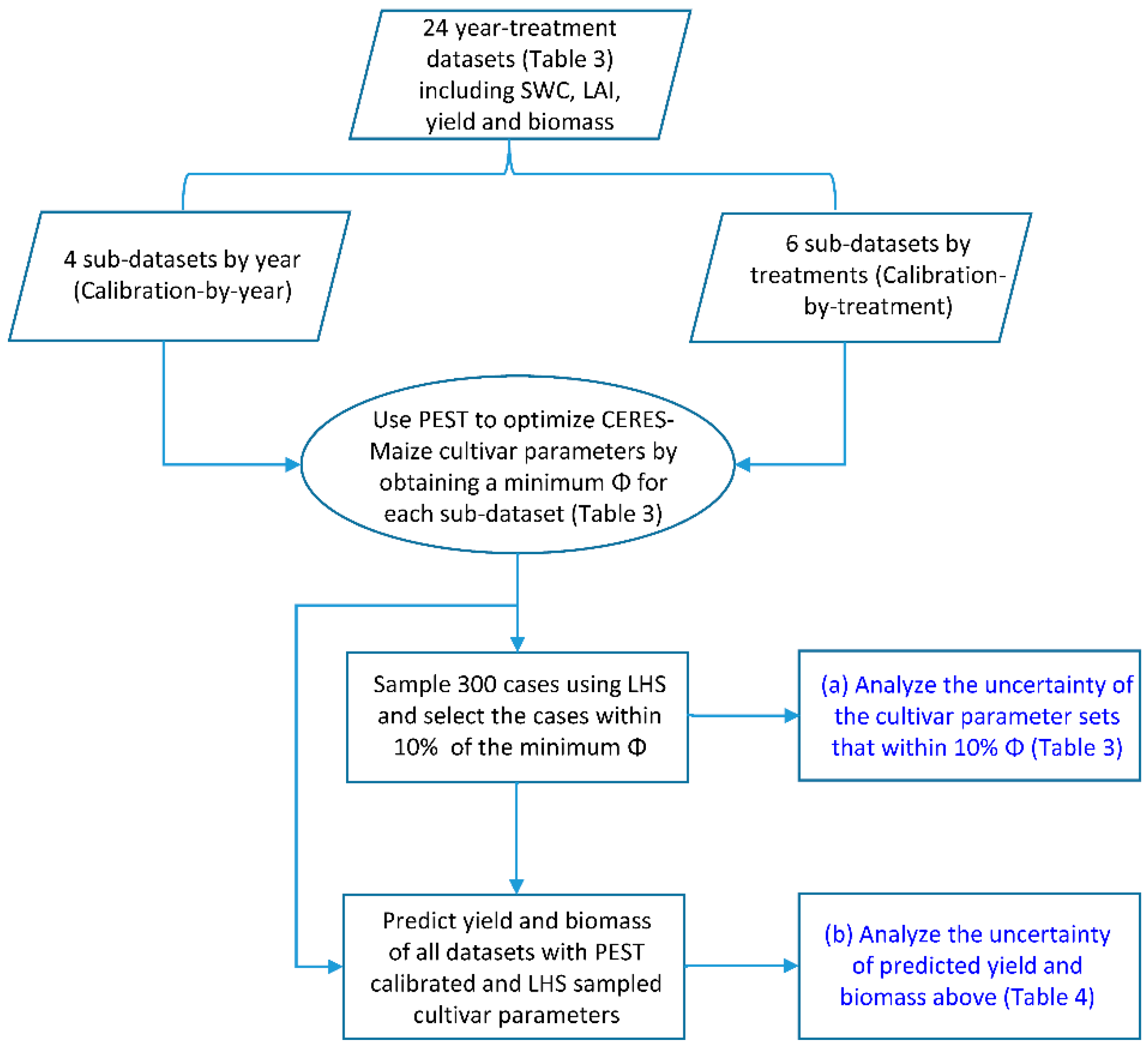
2.2. RZWQM2 Calibrations with PEST

The Root Zone Water Quality Model (RZWQM2, version 2.6) is a process-based, one-dimensional, field-scale model that produces detailed simulations of soil water, soil temperature, plant growth, pesticide fate, and soil carbon and nitrogen dynamics as influenced by various agricultural management practices [32]. The Green-Ampt equation is used for soil water infiltration and the Richards’ equation for soil water redistribution. The modified Brooks-Corey equations [33] are used to describe the soil water retention curve in the model. The CERES-Maize crop model incorporated into RZWQM2 is used to simulate crop growth, water use, and N uptake in this study, where RZWQM2 provides soil water, soil temperature, and nutrient information for the DSSAT4.0 crop models [34].
An automated parameter estimation software (PEST), described by Doherty [14], was incorporated into RZWQM2 to facilitate model calibration. PEST uses a hybrid method of Tikhonov regularization and truncated singular value decomposition (SVD) regularization for calibration [14]. The objective function (Φ) is expressed in general form as [7,14]:
Φ ( b ) = [ y y ( b ) ] T Q [ y y ( b ) ] ,
where Q is a weight matrix, y is a vector of observations, y′(b) is a vector of simulated values produced by the model based on parameter vector b, and T indicates matrix transpose. Both y and y′(b) have the same dimension. Parameters that minimize this equation are attained by solving the normal equations using the Gauss-Marquardt-Levenberg (GML) gradient search algorithm [14]. In this study, the objective function is the sum of squared errors between experimental and simulated yield, biomass, LAI, and soil water content.
The CERES-Maize cultivar parameters (Table 1) were selected for optimization to investigate the effect of different sub-datasets on calibrated crop parameters and subsequent prediction of crop yield and biomass. Other parameters (such as soil hydraulic parameters) were from previous publications without modification [35]. The initial crop parameters and their ranges used in PEST were the same as those in Sima et al. [23] based on reported values in the literature [7,35], except for the field capacity, which was from Ma et al. [35] (Table 2). For model calibration, the 24 year-by-treatment data points were sub-divided into four groups by year (Year_08, Year_09, Year_10, and Year_11) (Calibration-by-Year) or into six groups by treatments (Treat_T1, Treat_T2, Treat_T3, Treat_T4, Treat_T5, and Treat_T6) (Calibration-by-Treatment). Data that were not used for model calibration were used for model validation. The overall prediction of all datasets was compared among the two calibration methods (Figure 1).
A sensitivity analysis of model outputs (soil water content, LAI, grain yield and biomass across all the six treatments and four years) to the crop cultivar parameters were conducted with PEST, where a composite sensitivity of each parameter was calculated by normalized magnitude with respect to the number of observations [14]. The composite sensitivity of any parameter can be considered as the magnitude of the vector comprising the column of the Jacobian matrix (the derivatives of all model outputs with respect to a particular parameter), divided by the number of observations [14]. In this way, the effects of the different parameters (different types and magnitudes) on the model outputs can be compared. As shown in Table 1, soil water content showed low sensitivity to all the crop parameters, and low sensitivity of LAI to these crop parameters were also found, except for P1 and PHINT. Grain yield and biomass showed obviously higher sensitivities to the crop parameters than soil water content (SWC) and leaf area index (LAI) (Table 1). Of the six crop parameters, lowest sensitivities of simulated grain yield and biomass to P2 were found for the single location simulations (Table 1).

2.3. Unicertainty Analysis of Crop Parameters and Model Predictions

To quantify the uncertainties in model calibration and prediction, a Jacobian matrix was generated based on the optimized parameters from calibration by PEST’s RANDPAR utility, which was used to run the PREDUNC7 utility in PEST for the posterior covariance matrix [14]. During this procedure (Figure 1), 300 cases of six crop cultivar parameters were generated from LHS by assuming a normal distribution of each parameter within their respective reported ranges in the literature (Table 1). The LHS is modified from Monte Carlo method and showed higher efficiency than the original Monte Carlo simulation in sampling parameters with a given distribution [26]. Ma et al. [27] recommended a sampling size of 100 to quantify RZWQM sensitivity to both soil and crop cultivar parameters. The 300 cases generated by LHS method in this study should be adequate for the model uncertainty analysis considering the small crop cultivar parameter number (6 parameters in Table 1) and the highly efficient LHS method [26,27]. The parameter sets that provided Φ values within 10% of calibrated Φ (minimum Φ) values for the calibrated sub-dataset were selected to predict yield and biomass of the entire datasets (Figure 1), because we assumed a 10% deviation from the calibrated results as acceptable given the large experimental error in field measurements [7,28]. The selected cases within 10% of calibrated Φ may be different but reflect the model uncertainties associated with these different calibration sub-datasets, which were then used to quantify the uncertainty of crop parameters and predictions of yield and biomass for each calibrated sub-datasets (Figure 1).
The uncertainty of crop parameters associated with the scenarios within 10% of calibrated Φ, and subsequent prediction of yield and biomass were quantified with statistics of RMSE (root mean squared error, Equation (2)), relative RMSE (RRMSE = RMSE/mean, %) and coefficient of variation (CV, %; Equation (3)). In addition, the confidence intervals for the model predictions based on these selected cases were used to quantify the uncertainty in model predictions.
RMSE = 1 n i = 1 n ( P i O i ) 2 ,
CV = SD/Vavg × 100%,
where Pi is the ith simulated yield or biomass; Oi is the ith observed yield or biomass; n is the number of data pairs; SD is the standard deviation of the variable of interest and Vavg is the average value of the variable of interest.

3. Results and Discussion

3.1. Uncertainty in Model Calibration among Sub-Datasets

Previous simulations with the same model and datasets showed reasonable predictions of soil water contents, LAI, and crop phenology [6,7]. There was no great difference in simulated soil water content (RMSE = 0.034–0.035 cm3 cm−3) and LAI (RMSE = 0.84–1.01 cm2 cm−2) among these different calibration sub-datasets, as confirmed by the low sensitivities of these model outputs to crop cultivar parameters (Table 1). The RMSE values for simulated soil water contents and LAI were close to the previous simulation with RMSE = 0.030–0.039 cm3 cm−3 and 0.78–0.98 cm2 cm−2, respectively [6]. The RMSE values for the predicted crop anthesis date ranged from 2.6 to 6.0 days (average value = 4.5 days) for the Calibration-by-Year and from 3.4 to 5.1 day (average value = 4.3 days) for the Calibration-by-Treatment, which were also comparable to previous simulations using the same model and datasets [6,7]. The higher simulated RMSE values among the four Calibration-by-Year scenarios than the six Calibration-by-Treatment scenarios were expected since only one year data were used for the Calibration-by-Year.
For both Calibration-by-Year and Calibration-by-Treatment methods, PEST-optimized P1 (thermal time from seedling emergence to end of juvenile phase) and PHINT (thermal time for a leaf tip to emerge) had the lowest CV values, followed by P5 (grain filling duration, thermal time from silking to physiological maturity), G2 (potential kernel number), G3 (potential kernel growth rate), and P2 (day length sensitivity coefficient), among the individual scenarios in each group (Table 3). The high variability among Calibration-by-Year (CV = 94.8%) and among Calibration-by-Treatment (CV = 124.8%) for P2 indicated high uncertainty associated with the calibration data (grain yield and biomass) from different years or treatments but same location. The high uncertainty of P2 was mainly due to the low sensitivity of simulated grain yield and biomass to P2 under the current experimental conditions, and DeJonge et al. [4] also reported low sensitivity of grain yield and LAI to P2 and recommended that the default value of this parameter be used. Therefore, calibrating the parameter of P2 in CERES-Maize model should be caution especially using measured data from a single location. The average calibrated cultivar parameters between the two calibration methods were similar for P1, P2, and PHINT (Table 3). The other crop yield-related parameters (P5, G2, and G3) varied considerably between the two calibration methods and among the different calibration scenarios for each method (e.g., Year_08-Year_11 or Treat_T1-Treat_T6, Table 3), which indicated their high uncertainties when calibrating the model using the final crop yield and biomass. However, these parameter uncertainty could be reduced if more yield related measurements (such as kernel weight and kernel number) were available. The higher CV values among Calibration-by-Year than among Calibration-by-Treatment for P5 (26.5% vs. 14.0%) and G2 (28.1% vs. 22.8%) suggested higher uncertainty due to weather variability than to irrigation amounts. Another crop yield related parameter, G3, showed slightly lower CV values among Calibration-by-Year than among Calibration-by-Treatment (39.0% vs. 44.5%, Table 3), mainly due to the higher calibrated G3 value (reaching the upper end of the range of acceptable values for G3) for Treat_T6 calibration scenarios.
Similar to the results of Sima et al. [23], PEST was able to calibrate biomass and yield well when calibrating the model with either all of the treatments in one year (Calibration-by-Year) or one treatment in all years (Calibration-by-Treatment). The RMSEs for simulated grain yield and biomass were 1232–2560 kg ha−1 and 1817–2819 kg ha−1, respectively, for the Calibration-by-Year scenarios, and were 876–1194 kg ha−1 and 1542–2068 kg ha−1, respectively, for Calibration-by-Treatment scenarios (Table 4). The corresponding RRMSE values were 15%–30% (grain yield) and 11%–16% (biomass) for the Calibration-by-Year scenarios and 10%–14% (grain yield) and 9%–12% (biomass) for Calibration–by- Treatment scenarios.
Across the four Calibration-by-Year scenarios (Year_08 to Year_11, Table 4), the RMSEs showed higher variability for grain yield (CV = 35%) than for aboveground biomass (CV = 20%). The calibration with the sub-dataset of Year_09 produced slightly higher RMSE and RRSME values for both grain yield and biomass, compared with other years (Year_08, Year_10, and Year_11, Table 4). Across the six Calibration-by-Treatment scenarios (Treat_T1 to Treat_T6) (Table 4), the RMSE values showed lower variabilities (CV = 11%) for both grain yield and biomass, compared with the Calibration-by-Year results. These results indicated lower uncertainty by the method of Calibration-by-Treatment than that of Calibration-by-Year, which agrees with previously published results [23,24,25].

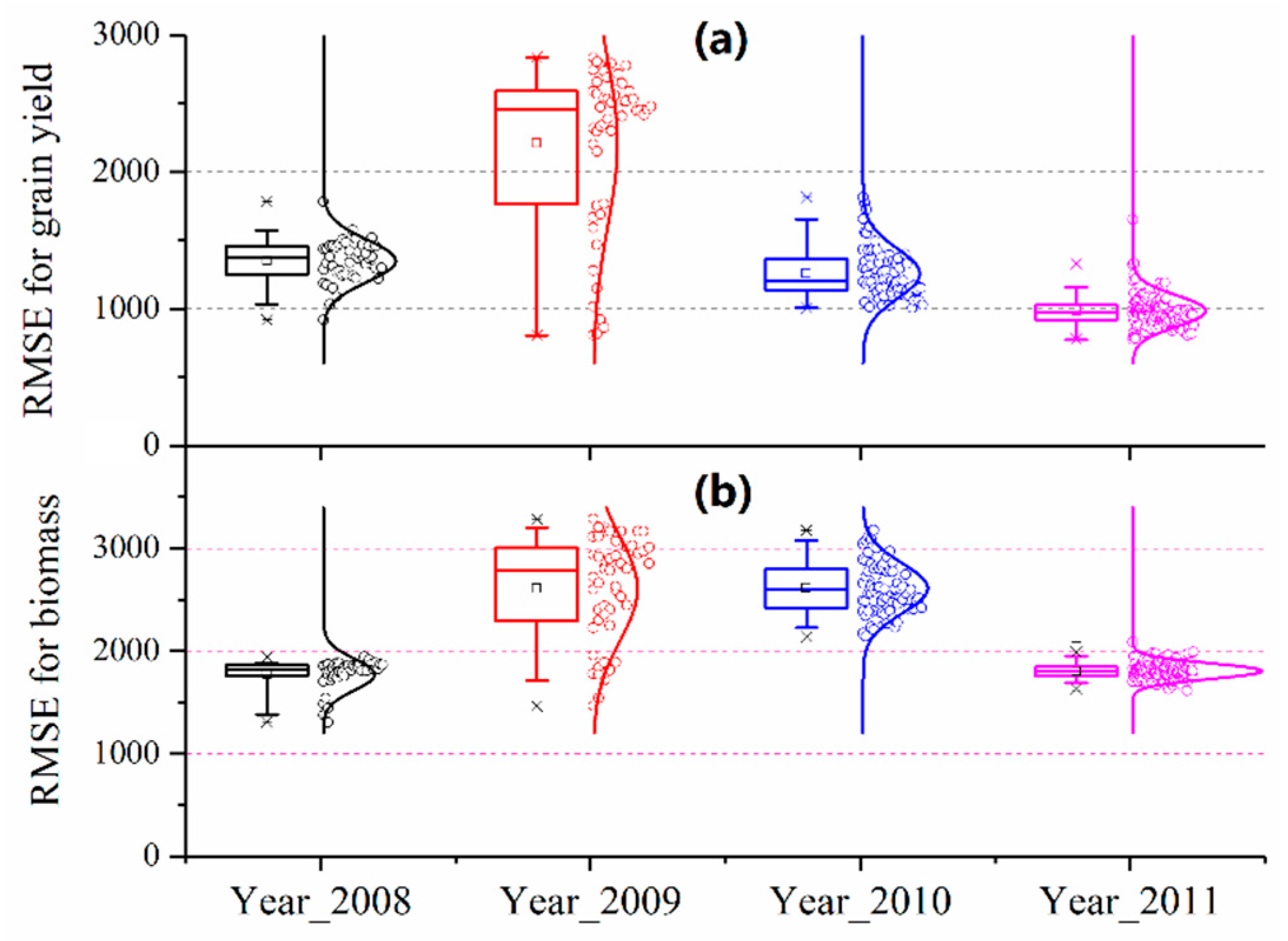
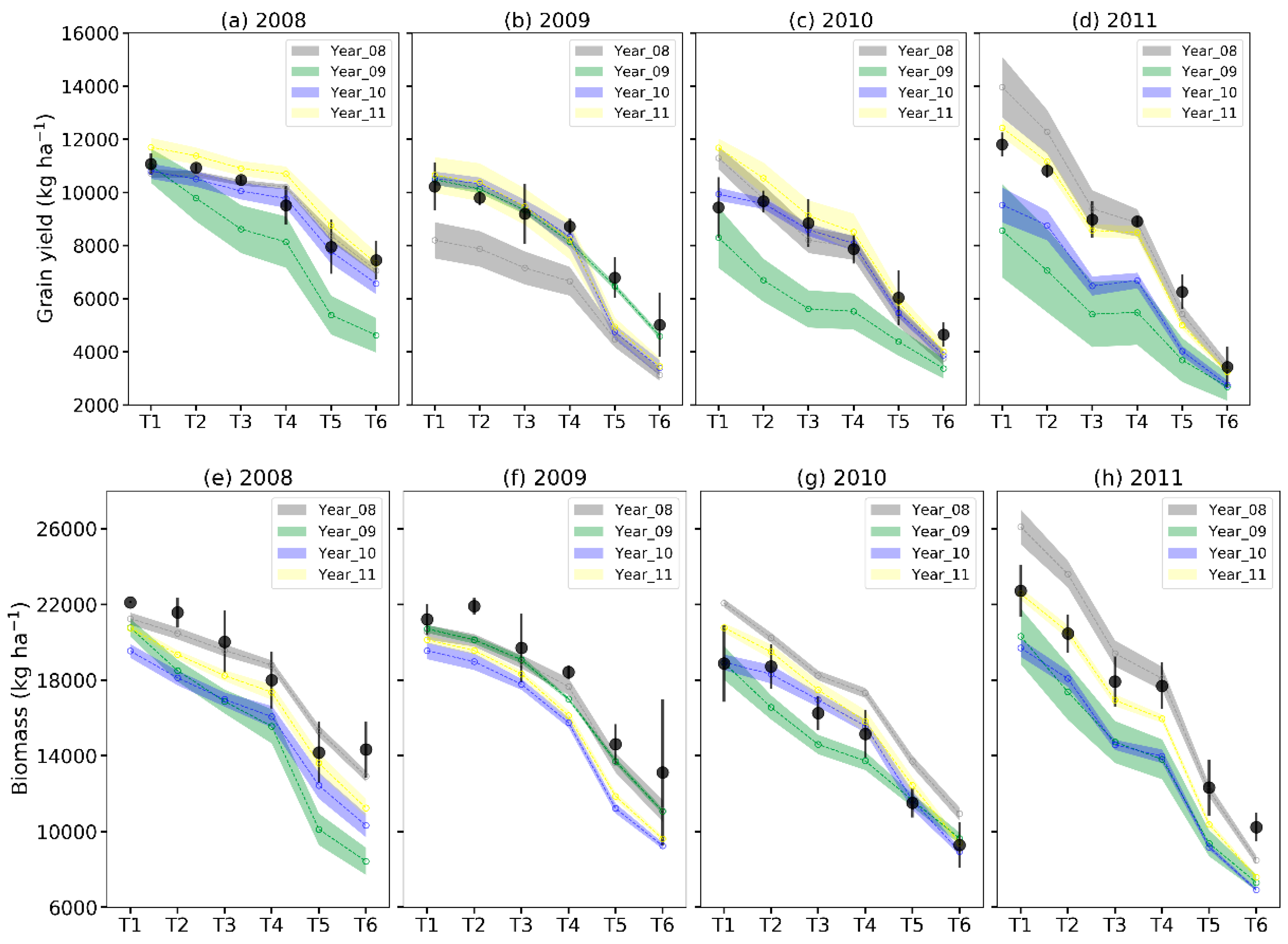
3.2. Uncertainty in Model Predicitions Based on Calibration-By-Year Method

Among the 300 sampled cultivar parameter sets, 44, 50, 74, and 151 sets simulated Year_08, Year_09, Year_10, and Year_11 sub-datasets adequately within 10% of calibrated minimum Φ values, respectively. The variability in crop parameters among the selected Φ cases for each Calibration-by-Year scenario is shown in Table 3 and Figure 2. Across the four calibration scenarios, the averaged parameter values from the selected Φ cases were relatively stable for P1 (CV = 7.8%) and PHINT (CV = 14.4%), and varied greatly for P2 (CV = 99.5%). The CV values were 21.6% for P5, 25.6% for G2, and 23.3% for G3. These variations were similar to those during PEST optimization as shown in Table 3. For the Year_08 sub-dataset, G2 and G3 were relatively stable among the scenarios with CV values of 6.2% and 6.8%, respectively, whereas they varied greatly among the Φ cases for other three sub-datasets (CV = 16.6%–26.4% for G2 and 17.4%–22.0% for G3, Table 3). Opposite trends were true for P1, P2, P5, and PHINT across the calibration years, with high variation among the cases for Year_08 (CV = 6.6, 35.6, 15.3, and 5.6%, respectively), and low variation for other calibration years (Figure 2 and Table 3). This result showed high parameter uncertainty associated with the compensations among these cultivar parameters when calibrating them using final grain yield and biomass data only.
The RMSE values for simulated grain yield among the selected Φ cases ranged from 918 to 1782 kg ha−1, 806 to 2836 kg ha−1, 1006 to 1814 kg ha−1, and 773 to 1651 kg ha−1 with CV values of 11%, 47%, 15%, and 11%, for Year_08, Year_09, Year_10, and Year_11, respectively (Figure 3). The corresponding RMSEs for simulated aboveground biomass ranged from 1307 to 1942 kg ha−1, 1465 to 3285 kg ha−1, 2141 to 3176 kg ha−1, and 1614 to 2087 kg ha−1, with CV values of 9%, 19%, 9%, and 4% (Figure 3). Among the four calibration scenarios, higher RMSE and RRMSE values for both grain yield and biomass with higher variation (higher CV values) were simulated for Year_09 than for other calibration years (Figure 3 and Table 4). This result was generally consistent with the optimization results with different calibration years (Table 4) and was probably due to the higher variation in the calibrated parameters of G2 and G3 among the selected Φ cases in 2009 (CV values of 19.8%-26.4%) than in other years (CV values of 6.2%–22.0%) (Figure 2 and Table 3).
The uncertainty in yield and biomass predictions in terms of CV among the selected Φ cases is generally lower for calibration than for validation (Figure 4). Among the four calibration year scenarios, predicted uncertainty in yield and biomass was higher for Year_09 and lower for Year_11. Year_09 greatly under-predicted crop yield and biomass than other three years (Year_08, Year_10, and Year_11; Figure 4a,c,d and Figure 4e,g,h). Year_08 greatly under-predicted grain yield in 2009 (Figure 4b) but over-predicted biomass in 2010–2011 (Figure 4g,h). Year_10 greatly under-predicted grain yield and biomass in 2011 (Figure 4d,h). Year_11 showed better yield and biomass predictions with lower uncertainty and lower RMSEs compared with the other three years (Figure 4 and Table 4). In addition, the uncertainty of predicted biomass was generally lower than the uncertainty in predicted grain yield (Figure 4a–d vs. Figure 4e–h; Table 4).

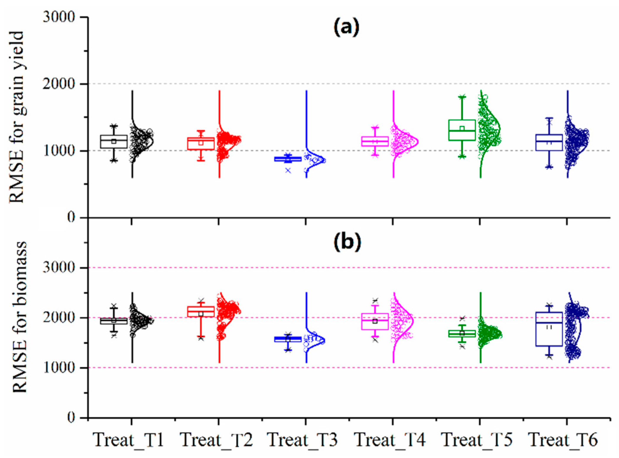
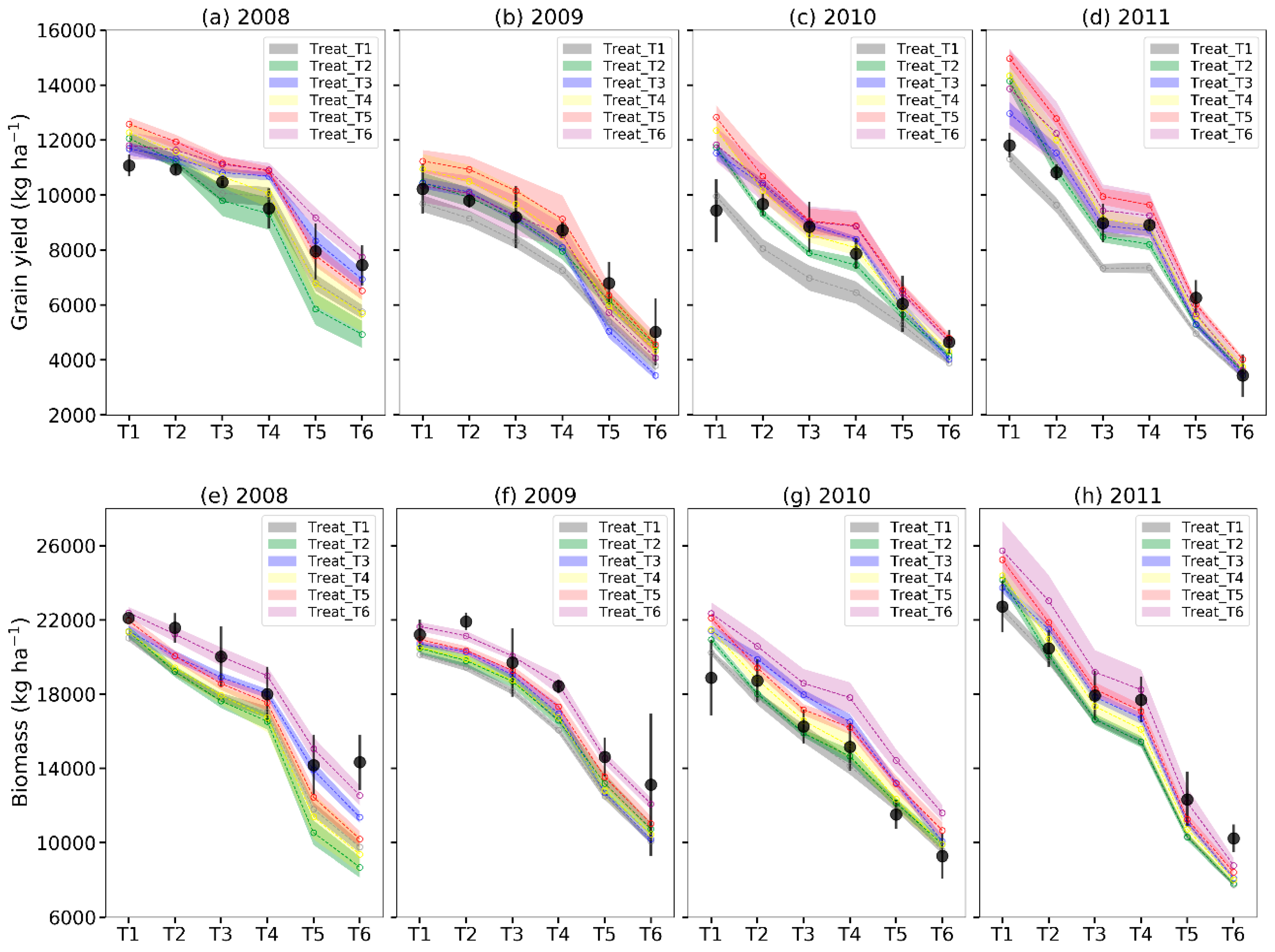
3.3. Uncertainty in Model Predicitons Based on Calibration-by-Treatment Method

There were 77, 140, 11, 45, 99, and 164 cases within 10% of calibrated Φ values for the Treat_T1 to Treat_T6 sub-datasets, respectively. The crop parameter variability among the selected cases for the Calibration-by-Treatment method was lower (more stable) compared with that for the Calibration-by-Year method (Figure 2 and Figure 5; Table 3). The CV values were below 15% for most of the crop parameters with the exception of P2 which had CV values from 20.6% to 79.5% for the six Calibration-by-Treatment scenarios (Figure 5; Table 3). Among the six calibration scenarios (Figure 5), the average crop parameters from the selected Φ cases showed similar variability to the PEST-optimized crop parameters, with CV values of 5.2% for P1, 128.1% for P2, 13.0% for P5, 22.6% for G2, 46.0% for G3, and 6.0% for PHINT (Table 3).
The calibration of Treat_T6 resulted in higher values of P2 and G3 but lower values of G2 among the selected Φ cases, compared with the other calibration treatments (Figure 5 and Table 3), which suggested high uncertainty in optimized crop parameters when the model was calibrated with the most severe water stress treatment (i.e., Treat_T6, irrigated to replace only 40% of potential crop ET). If only considering the no water stress or lower water stress treatments for calibration (i.e., Treat_T1-Treat_T5), the variability in crop parameters across the six Calibration-by-Treatment scenarios were reduced considerably with CV values below 16%.
Compared with the Calibration-by-Year (Figure 3), the RMSEs among the selected Φ cases were generally lower for both grain yield (average RMSE values: 1118 vs. 1482 kg ha−1) and biomass (average RMSE values: 1831 vs. 2198 kg ha−1) using the Calibration-by-Treatment method (Table 4 and Figure 6). The variability among the selected Φ cases for the Calibration-by-Treatment was lower for simulated grain yield (average CV values: 11% vs. 21%) but similar for simulated biomass (average CV values: 10% vs. 10%), compared with that for the Calibration-by-Year (Table 4). These results indicated a lower uncertainty in yield and biomass predictions based on the Calibration-by-Treatment method than that based on the Calibration-by-Year method. The estimated uncertainty in yield and biomass prediction (CV values from 7%–47% for grain yield and 4%–19% for biomass) were generally higher than measurement error of 7.5%, which suggested that the model could have performed even better if the higher simulation uncertainty in this study had been used in the F-test of Sima et al. [23].
Besides higher CV of crop parameters, the RMSE values for yield and biomass prediction showed higher variability among the selected Φ cases for Treat_T6 (CV = 14% for grain yield and CV = 19% for biomass) (Table 4 and Figure 6). Therefore, calibration data from severe water stress treatments could result in higher uncertainty of model parameters (Figure 5) and predictions of yield and biomass (Figure 6). Consequently, data acquired from less water stressed treatments should be used for calibration, as recommended by Boote et al. [36]. Reduced uncertainty for predicting crop yield and biomass can be obtained by calibrating two treatments across multiple years (such as both T1 and T6 across the four years) as confirmed by a previous simulation study on deficit irrigation management in the North China Plain [37].
Further comparisons of the uncertainty in model prediction estimated from standard deviations among these selected Φ cases is shown in Figure 7. Similar to the uncertainty in Calibration-by-Year (Figure 4), lower uncertainty was generally simulated for calibration than for validation, and for biomass prediction (Figure 7e–h) than for grain yield prediction (Figure 7a–d). Compared with the Calibration-By-Year results, lower uncertainty in predicted grain yield (average CV values of 11% and 21%) but similar uncertainty in predicted biomass (average CV values of 10% and 10%) were found for the Calibration-by-Treatment (Figure 4 vs. Figure 7; Table 4). Among the six Calibration-by-Treatment scenarios, higher uncertainty in yield and biomass prediction occurred for Treat_6 (CV = 19%) than for Treat_T1-Treat_T5 (CV = 6%–11%; Table 4). The high prediction uncertainty was simulated mainly for the high irrigation treatments with over-predicted grain yield and biomass (i.e., Treat_1-Treat_2 in 2010–2011, Figure 7c,d,g,h). Similarly, over-predicted grain yield for Treat_1-Treat_2 in 2008–2011 was also found for the Treat_T4 and Treat_T5 (Figure 7c,d). On the other hand, the Treat_T1 and Treat_T2 with low uncertainties also greatly under-predicted grain yield for the low irrigation treatments (Figure 7a–d), which was in agreement with previous study with the CERES-Maize model as reported by Marek et al. [38] and Liu et al. [39]. The worse simulations after model calibrations as shown in Figure 4 and Figure 7, partly due to only part of the datasets for calibration, had little effect on the model uncertainty assessment since the overall errors (RMSE and RRMSE) from both calibration and validation were used for each calibration scenario (Figure 1).

4. Conclusions

In this study, we demonstrated how simulation uncertainty varied with data selection for model calibration using PEST optimization algorithm and the LHS sampling technique. The results showed that the crop cultivar parameters calibrated using experimental data from one treatment (full irrigation or deficit water stress treatments) across all four years (Calibration-by-Treatment method) resulted in better yield and biomass predictions than those derived using data from all treatments in one year (Calibration-by-Year method). Higher variation in calibrated crop cultivar parameters among the selected Φ cases (within 10% of calibrated Φ values) were simulated for the Calibration-by-Year method than for the Calibration-by-Treatment method. These results indicated that uncertainty in model prediction was due more to year variability than to treatment effects (irrigation) under the current experimental conditions. Therefore, when crop parameters are calibrated from measured yield and biomass only, parameter uncertainty should be reported and used to generate confidence intervals of model predictions resulting from parameter uncertainty. Our results also suggested that simulation uncertainty could be reduced when the model was calibrated with experimental data covering a wide range of management and weather conditions.

Author Contributions

Conceptualization, Q.F., L.M., and R.D.H.; methodology, P.N.S.B. and M.W.S.; software, J.D. and P.N.S.B.; writing—Q.F. and L.M.; writing—review and editing, R.W.M., B.T.N., and Q.Y.

Funding

This work was supported in part by the CAS “Light of West China” Program, the National Key Research and Development Program (2016YFD030083) and the National Natural Science Foundation of China (31671627).

Acknowledgments

The authors wish to thank Roger Marquez and Bruce Vandenberg for their help in PEST optimization.

Conflicts of Interest

The authors declare no conflict of interest. The funding sponsors had no role in the design of the study; in the collection, analyses, or interpretation of data; in the writing of the manuscript; and in the decision to publish the results.

References

  1. Ahuja, L.R.; Ma, L. Parameterization of agricultural system models: Current approaches and future needs. In Agricultural System Models in Field Research and Technology Transfer; Ahuja, L.R., Ma, L., Howell, T.A., Eds.; Lewis Publishers: Boca Raton, FL, USA, 2002; pp. 273–316. [Google Scholar]
  2. Madsen, H. Parameter estimation in distributed hydrological catchment modelling using automatic calibration with multiple objectives. Adv. Water Resour. 2003, 26, 205–216. [Google Scholar] [CrossRef]
  3. Beven, K.; Binley, A. The future of distributed models: Model calibration and uncertainty prediction. Hydrol. Process. 1992, 6, 279–298. [Google Scholar] [CrossRef]
  4. DeJonge, K.C.; Ascough, J.C.; Ahmadi, M.; Andales, A.A.; Arabi, M. Global sensitivity and uncertainty analysis of a dynamic agroecosystem model under different irrigation treatments. Ecol. Model. 2012, 231, 113–125. [Google Scholar] [CrossRef]
  5. Fang, Q.X.; Green, T.R.; Ma, L.; Erskine, R.H.; Malone, R.W.; Ahuja, L.R. Optimizing soil hydraulic parameters in RZWQM2 under fallow conditions. Soil Sci. Soc. Am. J. 2010, 74, 1897–1913. [Google Scholar] [CrossRef]
  6. Ma, L.; Trout, T.J.; Ahuja, L.R.; Bausch, W.C.; Saseendran, S.A.; Malone, R.W.; Nielsen, D.C. Calibrating RZWQM2 model for maize responses to deficit irrigation. Agric. Water Manage. 2012, 103, 140–149. [Google Scholar] [CrossRef]
  7. Ma, L.; Ahuja, L.R.; Saseendran, S.A.; Malone, R.W.; Green, T.R.; Nolan, B.T.; Bartling, P.N.S.; Flerchinger, G.N.; Boote, K.J.; Hoogenboom, G.A. Protocol for parameterization and calibration of RZWQM2 in field research. In Methods of Introducing System Models into Agricultural Research; Ahuja, L.R., Ma, L., Eds.; SSSA book series; American Society of Agronomy, Inc.; Crop Science Society of America, Inc.; Soil Science Society of America, Inc.: Madison, WI, USA, 2011; pp. 1–64. [Google Scholar]
  8. He, J.; Jones, J.W.; Graham, W.D.; Dukes, M.D. Influence of likelihood function choice for estimating crop model parameters using the generalized likelihood uncertainty estimation method. Agric. Syst. 2010, 103, 256–264. [Google Scholar] [CrossRef]
  9. Harmel, R.D.; Smith, P.K. Consideration of measurement uncertainty in the evaluation of goodness-of-fit in hydrologic and water quality modeling. J. Hydrol. 2007, 337, 326–336. [Google Scholar] [CrossRef]
  10. Yen, H.; Wang, X.; Fontane, D.G.; Harmel, R.D.; Arabi, M. A framework for propagation of uncertainty contributed by parameterization, input data, model structure, and calibration/validation data in watershed modeling. Environ. Modell. Softw. 2014, 54, 211–221. [Google Scholar] [CrossRef]
  11. Shan, S.; Wang, G.G. Survey of modeling and optimization strategies to solve high-dimensional design problems with computationally-expensive black-box functions. Struct. Multidiscip. Optim. 2010, 41, 219–241. [Google Scholar] [CrossRef]
  12. Duan, Q.Y.; Sorooshian, S.; Gupta, V. Effective and Efficient Global Optimization for Conceptual Rainfall-Runoff Models. Water Resour. Res. 1992, 28, 1015–1031. [Google Scholar] [CrossRef]
  13. Yang, J.; Reichert, P.; Abbaspour, K.C.; Xia, J.; Yang, H. Comparing uncertainty analysis techniques for a SWAT application to the Chaohe Basin in China. J. Hydrol. 2008, 358, 1–23. [Google Scholar] [CrossRef]
  14. PESThomePage.org-HOME PAGE; Doherty, J. PEST: Model-Independent Parameter Estimation. Available online: http://www.pesthomepage.org/ (accessed on 8 May 2019).
  15. Iizumi, T.; Yokozawa, M.; Nishimori, M. Parameter estimation and uncertainty analysis of a large-scale crop model for paddy rice: Application of a Bayesian approach. Agric. For. Meteorol. 2009, 149, 333–348. [Google Scholar] [CrossRef]
  16. Skahill, B.E.; Doherty, J. Efficient accommodation of local minima in watershed model calibration. J. Hydrol. 2006, 329, 122–139. [Google Scholar] [CrossRef] [Green Version]
  17. Fang, Q. Optimizing and uncertainty evaluation of soil and crop parameters in root zone water quality model. Trans. CSAE 2012, 28, 118–123, (in Chinese with English abstract). [Google Scholar]
  18. Ma, L.; Ahuja, L.R.; Nolan, B.T.; Malone, R.W.; Trout, T.J.; Qi, Z. Root Zone Water Quality Model (RZWQM2): Model use, calibration, and validation. Trans. ASABE 2012, 55, 1425–1446. [Google Scholar] [CrossRef]
  19. Wang, Q.J. The genetic algorithm and its application to calibrating conceptual rainfall-runoff models. Water Resour. Res. 1991, 27, 2467–2471. [Google Scholar] [CrossRef]
  20. Sumner, N.R.; Fleming, P.M.; Bates, B.C. Calibration of a modified SFB model for twenty-five Australian catchments using simulated annealing. J. Hydrol. 1997, 197, 166–188. [Google Scholar] [CrossRef]
  21. Marshall, L.; Nott, D.; Sharma, A. A comparative study of Markov chain Monte Carlo methods for conceptual rainfall-runoff modeling. Water Resour. Res. 2004, 40. [Google Scholar] [CrossRef] [Green Version]
  22. Ritter, A.; Muñoz-Carpena, R. Performance evaluation of hydrological models: Statistical significance for reducing subjectivity in goodness-of-fit assessments. J. Hydrol. 2013, 480, 33–45. [Google Scholar] [CrossRef]
  23. Sima, N.Q.; Harmel, R.D.; Fang, Q.X.; Ma, L.; Andales, A.A. A modified F-test for evaluating model performance by including both experimental and simulation uncertainties. Environ. Modell. Softw. 2018, 104, 236–248. [Google Scholar] [CrossRef]
  24. Thorp, K.R.; Batchelor, W.D.; Paz, J.O.; Kaleita, A.L.; DeJonge, K.C. Using cross-validation to evaluate CERES-Maize yield simulations within a decision support system for precision agriculture. Trans. ASABE 2007, 50, 1467–1479. [Google Scholar] [CrossRef]
  25. Fensterseifer, C.A.; Streck, N.A.; Baigorria, G.A.; Timilsina, A.P.; Zanon, A.J.; Cera, J.C.; Rocha, T.S. On the number of experiments required to calibrate a cultivar in a crop model: The case of CROPGRO-soybean. Field Crop. Res. 2017, 204, 146–152. [Google Scholar] [CrossRef]
  26. McKay, M.D.; Beckman, R.J.; Conover, W.J. A comparison of three methods for selecting values of input variables in the analysis of output from a computer code. Technometrics 1979, 21, 239–245. [Google Scholar]
  27. Ma, L.; Ascough, J.C., Jr.; Ahuja, L.R.; Shaffer, M.J.; Hanson, J.D.; Rojas, K.W. Root zone water quality model sensitivity analysis using the monte carlo simulation. Trans. ASAE 2000, 43, 883–895. [Google Scholar] [CrossRef]
  28. Moriasi, D.N.; Arnold, J.G.; van Liew, M.W.; Bingner, R.L.; Harmel, R.D.; Veith, T.L. Model evaluation guidelines for systematic quantification of accuracy in watershed simulations. Trans. ASABE 2007, 50, 885–900. [Google Scholar] [CrossRef]
  29. Trout, T.J.; Bausch, W.C. USDA-ARS Colorado maize water productivity data set. Irrig. Sci. 2017, 35, 241–249. [Google Scholar] [CrossRef]
  30. Allen, R.G.; Pereira, L.S.; Raes, D.; Smith, M. Crop Evapotranspiration-Guidelines for Computing Crop Water Requirements-FAO Irrigation and Drainage Paper 56; FAO: Rome, Italy, 1998; Volume 300, p. D05109. [Google Scholar]
  31. Allen, R.G.; Pereira, L.S.; Smith, M.; Raes, D.; Wright, J.L. FAO-56 dual crop coefficient method for estimating evaporation from soil and application extensions. J. Irrig. Drainage Eng.-ASCE 2005, 131, 2–13. [Google Scholar] [CrossRef]
  32. Ahuja, L.R.; Rojas, K.W.; Hanson, J.D.; Shaffer, M.J.; Ma, L. The Root Zone Water Quality Model; Water Resources Publication: Highlands Ranch, CO, USA, 2000. [Google Scholar]
  33. Brooks, R.; Corey, T. Hydraulic Properties of Porous Media. Hydrol. Pap. Colorado State Univ. 1964, 3, 1–27. [Google Scholar]
  34. Ma, L.; Hoogenboom, G.; Ahuja, L.R.; Ascough, J.C.; Saseendran, S.A. Evaluation of the RZWQM-CERES-Maize hybrid model for maize production. Agric. Syst. 2006, 87, 274–295. [Google Scholar] [CrossRef]
  35. Ma, L.; Ahuja, L.R.; Trout, T.J.; Nolan, B.T.; Malone, R.W. Simulating maize yield and biomass with spatial variability of soil field capacity. Agron. J. 2016, 108, 171–184. [Google Scholar] [CrossRef]
  36. Boote, K.J. Concepts for calibrating crop growth models. In 1999 DSSAT Version 3; Hoogenboom, G., Wilkens, P.W., Tsuji, G.Y., Eds.; University of Hawaii: Honolulu, HI, USA, 1999; Volume 4, pp. 179–199. [Google Scholar]
  37. Fang, Q.; Ma, L.; Qi, Z.; Shen, Y.; He, L.; Xu, S.; Kisekka, I.; Sima, M.; Malone, R.W.; Yu, Q. Optimizing Et-Based Irrigation Scheduling for Wheat and Maize with Water Constraints. Trans. ASABE 2017, 60, 2053–2065. [Google Scholar] [Green Version]
  38. Marek, G.W.; Marek, T.H.; Xue, Q.; Gowda, P.H.; Evett, S.R.; Brauer, D.K. Simulating evapotranspiration and yield response of selected corn varieties under full and limited irrigation in the Texas High Plains using DSSAT-CERES maize. Trans. ASABE 2017, 60, 837–846. [Google Scholar] [CrossRef]
  39. Liu, C.; Qi, Z.; Gu, Z.; Gui, D.; Zeng, F. Optimizing irrigation rates for cotton production in an extremely arid area using RZWQM2-simulated water stress. Trans. ASABE 2017, 60, 2041–2052. [Google Scholar] [CrossRef]
Figure 1. A schematic diagram for quantifying the uncertainty of crop parameters in CERES-Maize model and model predictions of yield and biomass for all the 24 year-treatment datasets (including soil water content (SWC), leaf area index (LAI), grain yield and biomass) in Table 3.
Agronomy 09 00241 g001
Figure 2. Variability in optimized maize cultivar parameters (P1, P2, P5, G2, G3, and PHINT as defined in Table 1) among the selected cases with Φ (objective function) values within 10% of calibrated minimum Φ values from the 300 cases generated by Latin hypercube sampling (LHS) for each Calibration-by-Year scenario. The boxplots show the minimum and maximum values (asterisks), medians (lines), and means (dots). The 25% and 75% percentiles are shown as the tops and bottoms of the boxes, and the 5% and 95% percentiles are shown as the whiskers below and above the boxes.
Agronomy 09 00241 g002
Figure 3. Box plots for RMSEs (Root Mean Square Error, kg ha−1) for simulated grain yield (a) and biomass (b) across the selected cases within 10% of calibrated minimum Φ values from the 300 cases generated by the Latin hypercube sampling (LHS) for Year_08, Year_09, Year_10, and Year_11. The boxplots show the minimum and maximum (asterisks), medians (lines), and means (dots). The 25% and 75% percentiles are shown as the tops and bottoms of the boxes, and the 5% and 95% percentiles are shown as the whiskers below and above the boxes.
Agronomy 09 00241 g003
Figure 4. Experimental and simulated grain yield (ad) and biomass (eh) for Year_08, Year_09, Year_10, and Year_11 based on the Calibration-by-Year method (Table 3). The vertical bars and shaded areas are ±1 Standard Deviation (SD) around the mean for experimental and simulation data, respectively. The SD values was calculated based on the replicates for measured data and on the selected Φ cases for simulated data.
Agronomy 09 00241 g004
Figure 5. Variation in optimized maize cultivar parameters (P1, P2, P5, G2, G3, and PHINT as defined in Table 1) among the selected cases within 10% of calibrated Φ values from the 300 cases generated by the Latin hypercube sampling (LHS) for Treat_T1 to Treat_T6 in Table 3. The boxplots show the minimum and maximum values (asterisks), medians (lines), and means (dots). The 25% and 75% percentiles are shown as the tops and bottoms of the boxes, and the 5% and 95% percentiles are shown as the whiskers below and above the boxes.
Agronomy 09 00241 g005
Figure 6. Box plots for RMSE (Root Mean Square Error, kg ha-1) values for simulated grain yield (a) and biomass (b) calculated from the selected cases within 10% calibrated minimum Φ values from the 300 cases generated by the Latin hypercube sampling (LHS) for Treat_T1 to Treat_T6 (Table 3). The boxplots show the minimum and maximum (asterisks), medians (lines), and means (dots). The 25% and 75% percentiles are shown as the tops and bottoms of the boxes, and the 5% and 95% percentiles are shown as the whiskers below and above the boxes.
Agronomy 09 00241 g006
Figure 7. Experimental and simulated yield (ad) and biomass (eh) for Treat_T1 to Treat_T6 based on the Calibration-by-Treatment method (Table 3). The vertical bars and shaded areas are ±1 Standard Deviation (SD) around the mean for experimental and simulation data, respectively. The SD values was calculated based on the replicates for measured data and on the selected Φ cases for simulated data.
Agronomy 09 00241 g007
Table 1. Sensitivity analysis of model outputs to these crop cultivar parameters, and their initial values and ranges as reported in the literature for the CERES (Crop Environment Resource Synthesis)-maize model in RZWQM2 (Root Zone Water Quality Model 2) [6,33].
Crop ParameterParameter Sensitivity AnalysisParameter Calibration
SWCLAIGrain YieldBiomassRangeInitial
P10.0040.233.435.38100–450250
P20.0000.000.020.030–20.2
P50.0030.062.802.38500–1000600
G20.0010.022.541.77440–1000900
G30.0010.032.902.065–166
PHINT0.0040.161.462.0338–5550
P1: Degree days (base temperature of 8 °C) from seedling emergence to end of juvenile phase (thermal degree days); P2: Day length sensitivity coefficient; P5: Degree days (base temperature of 8 °C) from silking to physiological maturity (thermal degree days); G2: Potential kernel number; G3: Potential kernel growth rate (mg per kernel per day); PHINT: Degree days required for a leaf tip to emerge (phyllochron interval) (thermal degree days).
Table 2. Soil horizon, soil bulk density, saturated soil water content, and calibrated field capacity used in previous studies [6,33].
Soil Depth (cm)Soil Bulk Density (g cm−3)Saturated Soil Water Content (cm3 cm−3)Field Capacity (cm3 cm−3)
0–151.4920.4370.231
15–451.4920.4370.242
45–751.4920.4370.230
75–1051.5680.4080.206
105–1351.5680.4080.205
130–1651.6170.3900.263
160–1901.6170.3900.310
Table 3. Calibrated cultivar parameter values, and the averaged cultivar parameter values and their coefficients of variation (CV, %) among the selected Φ cases (11–164 cases with Φ values within 10% of calibrated Φ values for each scenario) from the 300 cases generated by Latin hypercube sampling (LHS), for the Calibration-by-Year and Calibration-by-Treatment.
Calibration MethodsCalibration ScenariosCalibrated Parameter Values with PEST *Averaged Parameter Values from the Selected Φ Cases within 10% of Calibrated Φ Values and Their CV Values (in Parentheses, %) **
P1P2P5G2G3PHINTCase NumbersP1P2P5G2G3PHINT
All treatments in one year (Calibration-by-Year)Year_08283.30.76100045016.047.644287.2 (6.6)0.8 (35.6)904 (15.3)458 (6.2)15.1 (6.9)43.6 (5.6)
Year_09244.50.066176598.538.050241.9 (2.7)0.1 (35.0)669 (11.8)623 (26.4)9.0 (19.8)38.1 (0.9)
Year_10255.90.205559119.653.674248.4 (4.7)0.2 (37.1)544 (3.5)792 (22.5)12.2 (21.0)53.1 (2.5)
Year_11264.10.226339678.250.3151254.4 (5.5)0.2 (57.5)667 (3.9)838 (16.6)9.9 (22.0)49.8 (2.0)
Average259.60.296817779.747.9 258.0 (4.9)0.3 (41.3)696 (8.6)678 (17.9)11.6 (17.4)46.2 (2.7)
CV ***5.894.826.528.139.012.4 7.899.521.62623.314.4
One treatment for all years (Calibration-by-Treatment)Treat_T1258.40.197579975.744.977252. (2.1)0.2 (20.6)755 (3.5)981 (5.0)5.8 (7.3)44.2 (3.0)
Treat_T2239.90.2188910005.643.2140238.5 (0.9)0.2 (31.3)958 (6.1)966 (4.8)5.5 (9.1)39.8 (5.4)
Treat_T3279.30.066878938.345.311273.5 (3.5)0.1 (79.5)716 (5.4)856 (14.6)8.3 (17.6)44.5 (3.1)
Treat_T4237.30.019369516.843.545241.8 (7.3)0.02 (58.4)931 (8.8)916 (12.3)6.7 (14.8)42.1 (4.8)
Treat_T5249.90.2082510007.043.899241.1 (4.2)0.2 (62.8)986 (4.3)970 (6.4)7.0 (9.7)40.2 (4.5)
Treat_T6266.91.03100044116.039.8164251.1 (4.9)1.0 (43.5)839 (17.9)476 (14.9)15.5 (5.9)38.4 (1.9)
Average256.50.278318798.143.8 249.7 (3.8)0.3 (49.3)864 (7.6)861 (9.7)8.1 (10.7)41.5 (3.8)
CV ***5.9124.81422.844.54.7 5.2128.113.022.646.06.0
* P1: Degree days (base temperature of 8 8 °C) from seedling emergence to end of juvenile phase (thermal degree days); P2: Day length sensitivity coefficient; P5: Degree days (base temperature of 8 °C) from silking to physiological maturity (thermal degree days); G2: Potential kernel number; G3: Potential kernel growth rate (mg per kernel per d); PHINT: Degree days required for a leaf tip to emerge (phyllochron interval) (thermal degree days). ** the CV values were calculated from the selected Φ cases. *** the CV values were calculated among the four scenarios for Calibration-by-Year or among the six scenarios for Calibration–by-Treatment.
Table 4. The RMSE (root mean square error, kg ha−1) and relative RMSE (RRMSE, %) values for yield and biomass predictions using Parameter ESTimation (PEST) optimized cultivar parameters or LHS sampled cultivar parameters (11–164 cases with Φ values within 10% of calibrated minimum Φ values), for the Calibration-by-Year and Calibration-by-Treatment.
Calibration MethodsCalibration Scenarios with PESTYield and Biomass Predictions by PEST Optimized ParametersSelected Case NumbersYield and Biomass Predictions with the Optimized Parameters from the Selected Cases within 10% of Calibrated Φ Values
YieldBiomassYieldBiomass
RMSE *RRMSE *RMSE *RRMSE *RMSE **RRMSE **CV ***RMSE **RRMSE **CV ***
All dataInitial296435340320
Calibration-by-Year;
All treatments (T1–T6) in one year
Year_0813661618171144135016111770109
Year_09256030281916502337284726071519
Year_1012321524081474125615152610159
Year_1116241919951215198412111804114
Average169520226013 1482172121981310
Calibration-by-Treatment; One treatment for all years (2008–2011)Treat_T110781318821177113913101945116
Treat_T29841220681214011171392074129
Treat_T3876101568911865107155296
Treat_T411941418131145113413919291111
Treat_T51108131542999133216151679106
Treat_T61158131823111641121131418061119
Average106612178311 1118131118311110
* RMSE and RRMSE were calculated from all data sets (24 year-by-treatment data points) for each calibration scenario. ** RMSE and RRMSE values were calculated from all data sets (24 year-by-treatment data points) for each calibration scenario and then were averaged across the selected Φ cases (11–164 cases) for each calibration method. *** CV (coefficient of variation, %) values were calculated among the selected Φ cases (11–164 cases) for each calibration method.

