Automatic Classification of Chickpea Varieties Using Computer Vision Techniques

Abstract

There are about 90 different varieties of chickpeas around the world. In Iran, where this study takes place, there are five species that are the most popular (Adel, Arman, Azad, Bevanij and Hashem), with different properties and prices. However, distinguishing them manually is difficult because they have very similar morphological characteristics. In this research, two different computer vision methods for the classification of the variety of chickpeas are proposed and compared. The images were captured with an industrial camera in Kermanshah, Iran. The first method is based on color and texture features extraction, followed by a selection of the most effective features, and classification with a hybrid of artificial neural networks and particle swarm optimization (ANN-PSO). The second method is not based on an explicit extraction of features; instead, image patches (RGB pixel values) are directly used as input for a three-layered backpropagation ANN. The first method achieved a correct classification rate (CCR) of 97.0%, while the second approach achieved a CCR of 99.3%. These results prove that visual classification of fruit varieties in agriculture can be done in a very precise way using a suitable method. Although both techniques are feasible, the second method is generic and more easily applicable to other types of crops, since it is not based on a set of given features.

1. Introduction

Agriculture is a strategic sector of economies worldwide. The use of new technologies has proven effective in increasing production and reducing costs [1], specifically when applied in extensive cultivations, such as chickpeas (Cicer arietinum L). In fact, chickpea is one of the most extended crops in the world, that grows in more than fifty countries on five continents [2,3]. Chickpea is cultivated on 13.98 million hectares (594,489 in Iran, where data collection of this research took place), and the approximate total amount of production is 13.74 million tons (261,616 tons in Iran). 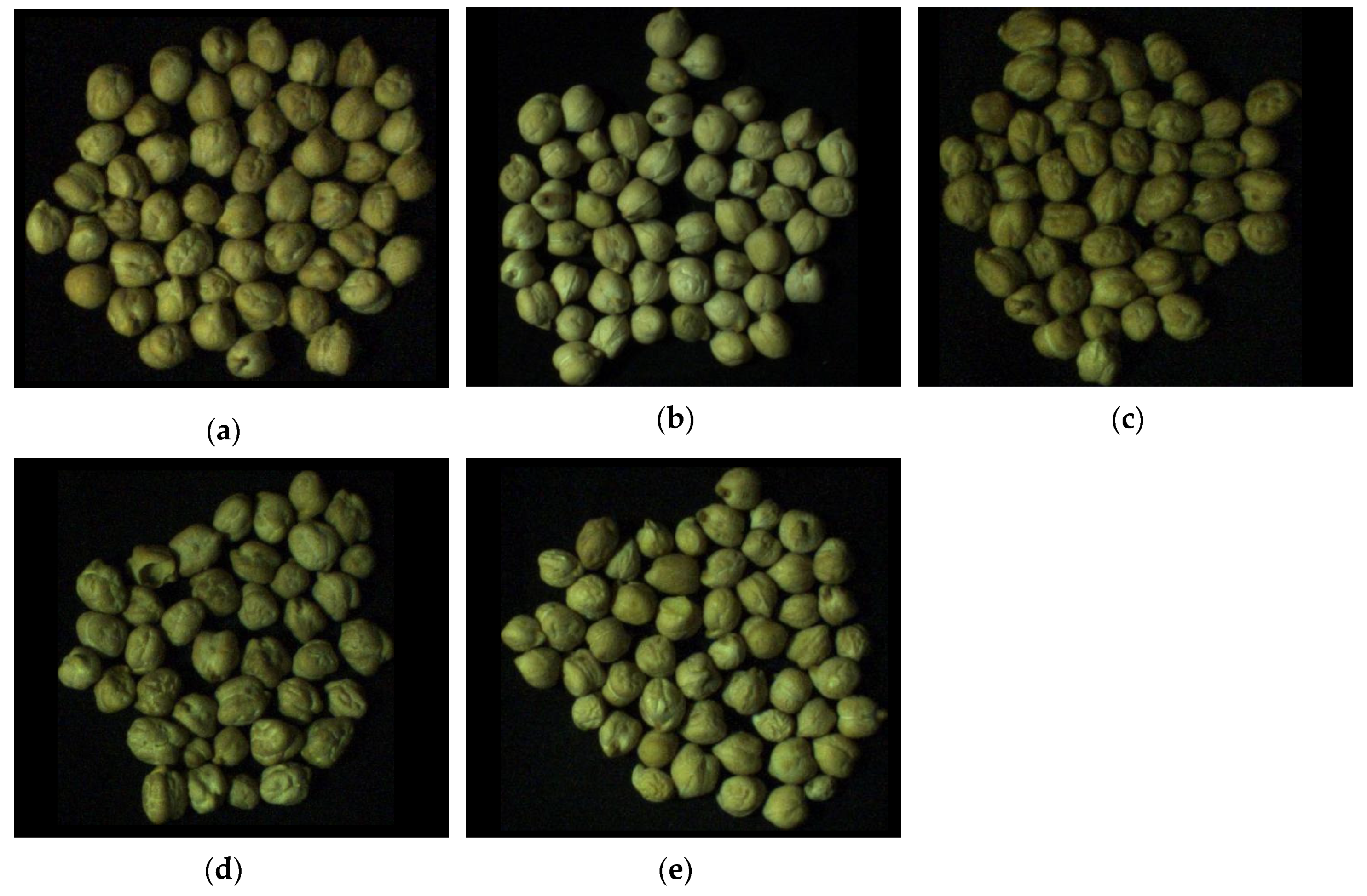Some researchers have studied the genotypes of up to 90 chickpea varieties [4], including wild varieties. There are five popular species of chickpeas in Iran: Adel, Arman, Azad, Bevanij and Hashem. Each type has a price and special applications in the food industry. However, the traditional method for detecting each variety of seeds is visual inspection by a human, which is a very tedious and time-consuming task [5,6].

Computer vision systems have a wide range of applications in agronomy and food industry such as irrigation, grading, harvesting, and automatic detection of different varieties of seeds as non-destructive assessment [7,8,9,10,11]. Some research works have used machine vision systems for the classification of different seeds [12]. For example, Aznan et al. [13] used machine vision methods to classify cultivated rice seed variety, namely M263, and weedy rice seed variants. These variants included: close panicle; partly short awned-open panicle; close panicle; partly short awned-close panicle; and partly long awned-close panicle for the seed industry. For this purpose, 120 samples of each variant and 600 samples of M263 were prepared. They used different morphological features such as solidity and extend for use in a stepwise discriminant function analysis (DFA) to classify different types of rice. Classification accuracy for testing and training sets were 96% and 95.8%, respectively. In addition, Kurtulmus et al. [14] proposed an algorithm for the classification of eight different varieties of pepper seeds based on machine vision combined with artificial neural networks (ANN). A total of 832 samples of these varieties were selected. After imaging, some color, shape and texture features were extracted from each sample. Then, these features were used as input to an ANN. The results showed that the accuracy of this classifier was 84.94%.

HemaChitra and Suguna [15] presented a new method based on image analysis techniques to discriminate defective from normal samples of Indian pulse seeds. For this purpose, they extracted several color, shape and texture features. Then, these features used as input to an SVM for classification. The result shows that the accuracy of their method was 98.9%. More recently, Li et al. [16] designed a system to discriminate different damaged types of corn. To do this, they used a database of images that included normal corn and six different damaged corns, such as blue eye mold-damaged and surface mold-damaged. The main techniques used are object segmentation, extraction of color and shape features, and a maximum likelihood classifier. In this case, the obtained classification accuracy was above 74% for all the classes.

As demonstrated in these papers, machine vision can be effectively used for seed classification, as an alternative to the traditional manual methods. They are able to increase accuracy and speed in packing and processing time. These systems use a classifier that is fed with features extracted from labelled data in order to learn the differences between distinct species or classes related to individual objects. On the other hand, there are several methods for selecting and classifying features, based on statistical and artificial intelligence methods, getting the latter more plausible results than the former due to non-sensitivity to the type of data distribution.

The main objective of the present research is to study and compare two different approaches in the selection of features in a particular task of fruit classification. The first method is based on a hybrid of artificial neural networks and the particle swarm optimization (PSO) metaheuristic algorithm. This method first extracts effective features from the data, by obtaining different color and texture information, in order to feed the classifier. 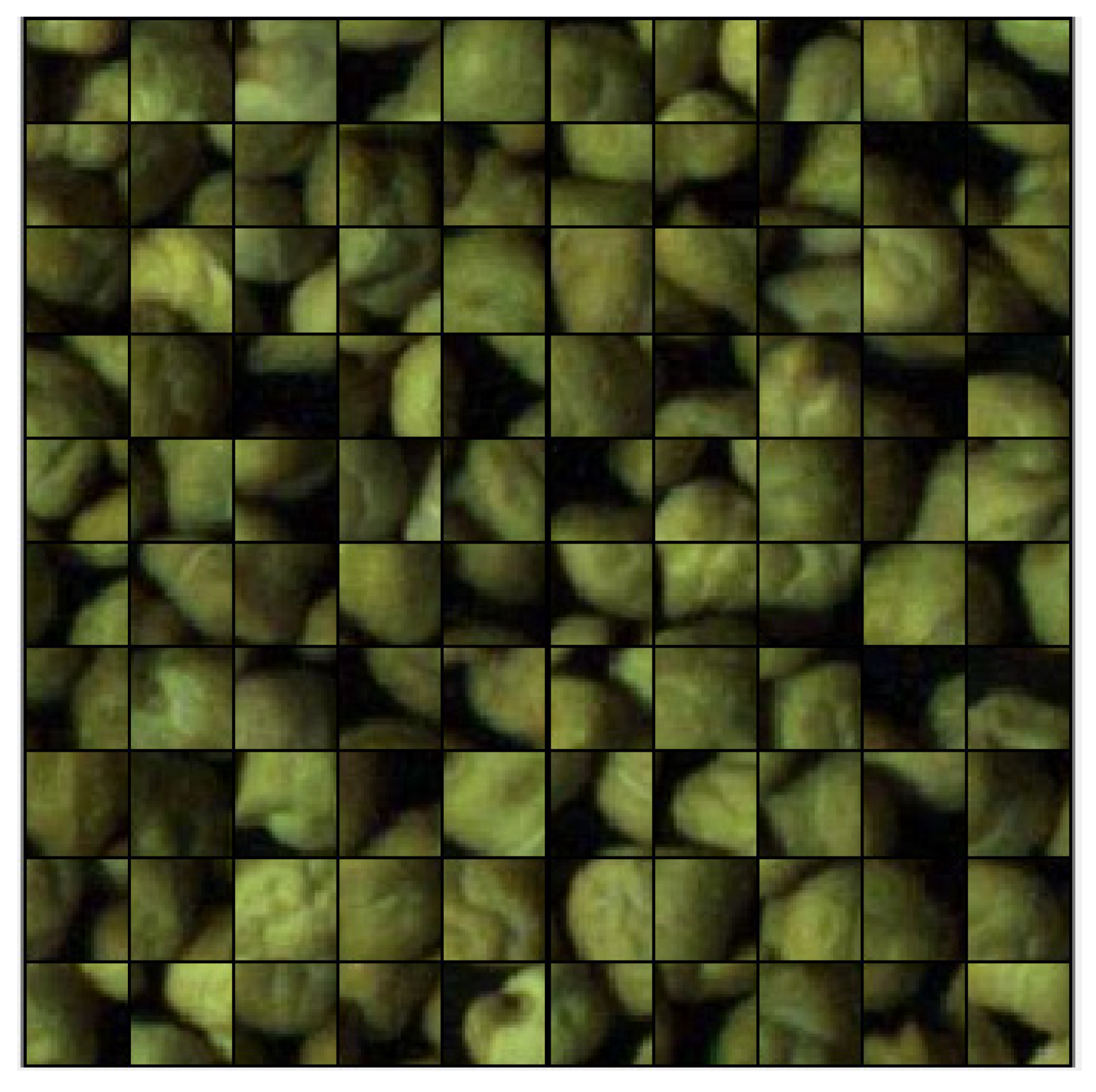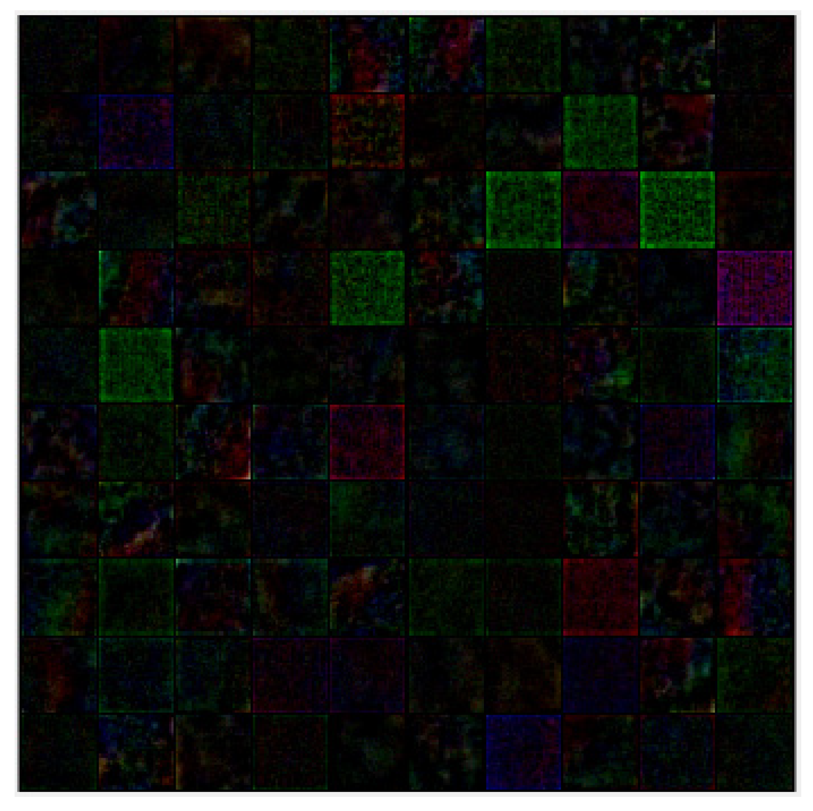The second approach can be referred to as a featureless method, since there is not an explicit feature extraction phase, but image patches are directly introduced into the classifier. These patches are the input of a three-layered (input, hidden and output layer) ANN, based on the classic feed-forward backpropagation algorithm [17].

Specifically, in this paper, the problem of interest is the classification of the five most common varieties of chickpeas in Iran. The samples were obtained in an Iranian zone in Kermanshah, with a total of 1019 images, by using an industrial camera from a 10 cm fixed height above the samples. This setup simulates the conditions of an industrial automatic classification device in a fruit processing factory. Both approaches, using features and not using features, are compared using the same data.

2. Materials and Methods

2.1. Data Collection of Chickpea Samples

As stated in the Introduction, there exist almost one hundred varieties of chickpeas. However, not all of them have commercial value, and the most used varieties depend on the geographical area. In this study, the 5 most common varieties of Iranian chickpeas were considered: Adel, Arman, Azad, Bevanij, and Hashem. The purpose is to design a precise computer vision method to classify images of these five different varieties, comparing two approaches based on standard computer vision techniques. The samples were obtained in Kermanshah, Iran (34°19′44.1″ N, 47°6′5.6″ E). Figure 1 shows one sample of each variety. It can be seen than they are visually very similar. Only with an expert eye and looking for details can they be distinguished.

To train and test the computer vision algorithms, a total of 1019 images were taken by using an industrial camera DFK 23GM021 (https://www.theimagingsource.com/products/industrial-cameras/gige-color/dfk23gm021/) (The Imaging Source GmbH, Bremen, Germany), that has a 1/3 inch CMOS (Complementary Metal Oxide Semiconductor) sensor able to capture at a maximum resolution of 1280 × 960 pixels and 60 frames per second. To simulate the conditions of a food processing factory, the images are captured from a 10 cm fixed height above the samples using a black background. Each image contains around 50 chickpeas; this number is approximate, since the chickpeas were not counted in each shot, and the actual number usually varies between 30 and 60 per image. The chickpeas are not isolated, but they are touching each other. This would be the case of a conveyor belt where chickpeas are transported continuously, passing under the camera at a certain point. After each capture, the chickpeas were removed and replaced with a different batch, i.e., chickpeas are not repeated in different images. White LED lamps with an intensity of 327 lux were used for lighting. In addition, 204 images were gathered for each variety type, except for the Arman variety, where one image was omitted.

2.2. Feature-Based Classification Method

The first approach is based on a classic structure consisting of 4 main steps: object segmentation; feature extraction; most effective features selection; and classification. Since this is a common approach currently applied in many works, we have considered it interesting to include it in this comparison of methods.

2.2.1. Segmentation of the Chickpeas

In order to segment the chickpeas with high accuracy, 5 color spaces were analyzed [18]. These color spaces are RGB, YIQ, HSV, HIS and YCbCr. The experimental results indicated that YCbCr was the optimal color space for segmentation, as it produced less noise in the samples available. The results also showed that two channels, Y and Cb, were the most suitable for thresholding. Therefore, the following equation is applied to segment chickpeas in each pixel:

$$\mathbf{if}Y\ge 20\mathrm{AND}Cb\le 15\mathbf{then}\mathrm{chickpea}\mathbf{else}\mathrm{background},$$

(1)

$$Y=0.299\times R+0.587\times G+0.114\times B;Cb=0.564\times \left(\mathrm{B}-\mathrm{Y}\right)+128$$

(2)

where R, G and B are the red, green and blue values of each pixel, respectively. That is, one pixel with Y smaller than 20, or Cb larger than 15 is considered as a part of the background. Otherwise, the pixel is assumed to belong to the objects. In order to remove some noise pixels in the background, morphology operator open was also used. Figure 2 shows all the stages of segmentation.

Since the experimental setup is prepared to facilitate segmentation, the results obtained are always very accurate. The segmentation error estimated in a subset of 10 sample images is below 0.15%. Since color information is extracted from the average of the segmented part of the image, the effect of this small error in subsequent processes is negligible.

2.2.2. Color and Texture Features Extraction

The main types of features used in the literature are color, texture and shape. However, in our case, shape cannot be precisely obtained since the chickpeas are crowded. Thus, two types of features were extracted, using color and texture; the latter are based on the gray level co-occurrence matrix (GLCM):

• Color features. All features in this type are divided into two groups: (1) statistical features, and (2) vegetation indices. Statistical features consist of the average and standard deviations of the 1st, 2nd and 3rd channels, and the average of them, using the RGB, YCbCr, YIQ, CMY, HSV and HSI color spaces—thus, 2 features × 4 channels × 6 color spaces = 48 features that were extracted from this group. Concerning the vegetation indices, they are a group of color features that have been proposed by other authors in computer vision in agriculture. Woebbecke et at. [19] proposed several indices, such as the additional green and green-minus-blue index, as a way of highlighting the pixels that are predominantly green. Other authors extended this idea to the additional red [20] and blue [21] indices, or the subtractive indices red-blue and green-red [21,22]. Some other indices have been created to help in segmentation of vegetation, such as the extracted vegetation cover index (CIVE) [23] and the normalized difference index (NDI) [24].

  Table 1. Color features used in the study related to vegetation indices.

  Extracted Color Index	Formula
  Normalized 1st component of RGB	$\begin{array}{c}{R}_n=R/\left(R+G+B\right)\end{array}$
  Normalized 2nd component of RGB	$G_n=G/\left(R+G+B\right)$
  Normalized 3rd component of RGB	$B_n=B/\left(R+G+B\right)$
  Gray channel	$gray=0.289R_n+0.587G_n+0.114B_n$
  Additional green	$EXG=2G_n-R_n-B_n$
  Additional red	$EXR=1.4R_n-G_n$
  Extracted vegetation cover	$CIVE=0.44R_n-0.81G_n+0.39B_n+18.8$
  Subtract of add. green and add. red	$EXGR=EXG-EXR$
  Normalized difference index	$NDI=\left(G_n-B_n\right)/\left(G_n+B_n\right)$
  Green index minus blue	$GB=\left(G_n-B_n\right)$
  Red-blue contrast	$RBI=\left(G_n-B_n\right)/\left(G_n+B_n\right)$
  Green-red index	$ERI=\left(R_n-G_n\right)\left(R_n-B_n\right)$
  Additional green index	$EGI=\left(G_n-R_n\right)\left(G_n-B_n\right)$
  Additional blue index	$EBI=\left(B_n-G_n\right)\left(B_n-R_n\right)$

  shows the computation of these indices for the RGB color space. These features were also extracted from YCbCr, YIQ, CMY, HSV and HSI color spaces. This way, the extracted features in this group were 14 features × 6 color spaces = 84.
• Texture features. The Gray Level Co-occurrence Matrix (GLCM) is a common technique to extract texture features from the images. 20 features (such as contrast, mean, variance and correlation) were extracted from 4 different angle neighborhoods, namely 0°, 45°, 90° and 135°, based on the GLCM. Therefore, 80 features were extracted in this group.

Summing up, there is a total of 48 + 84 + 80 = 212 color and texture features that are extracted for each image, considering the pixels segmented in the first step.

2.2.3. Selection of the Most Effective Features

The use of all 212 color and texture features extracted in the previous step as input to the classifier is not adequate, since they are not independent variables and all of them are computed from the RGB values. On the other hand, since the proposed application of non-destructive classification of chickpea varieties should be done in real time, extracting and using all the 212 features would be time-consuming, even if there is no contradiction between them. Therefore, it is necessary to choose the most effective features among the set of color and texture features.

In this study, the hybrid method of artificial neural networks and particle swarm optimization (ANN-PSO) was used to select the most effective features. In essence, the basic idea is testing different combinations of features with an ANN, being the combinations created with the PSO algorithm.

PSO is a meta-heuristic algorithm that emulates bird collective movements in order to optimize various issues. This algorithm was originally proposed by Kennedy and Eberhart [25]. Each answer—in our case, a combination of features—is considered as a little bird or particle. Each particle is constantly being searched and moved. The motion of each particle depends on three factors: (1) the current position of the particle; (2) the best position where that particle has already been; and (3) the best position that the whole set of particles has had. In this way, at first, all extracted features are considered as a vector. In the next step, smaller vectors of the features, for example, vectors with 3, 5 and 9 features, are selected by the PSO algorithm and sent to a multilayer perceptron neural network. The characteristics of this ANN are shown in

Table 2. Parameters of the ANN used in the ANN-PSO process to select the most effective features.

Feature	Value
Number of hidden layers	1
Number of neurons of the hidden layer	10
Transfer function	Hyperbolic tangent sigmoid
Backpropagation network training function	Levenberg-Marquardt backpropagation
Backpropagation weight / bias learning function	Hebb weight learning rule

.

The input of the neural network is the vector of features selected by the PSO, and the output is the corresponding chickpea variety. The available samples are divided by ratio of 70% for training, 15% for validation, and 15% for testing. For each execution of the ANN, the mean square error (MSE) of the test samples is recorded. Finally, the combination of features having the least MSE is selected as the optimal set of effective features.

In our case, the result of the ANN-PSO method was the selection of the following 6 most effective features: information measure of correlation for 135° angle; diagonal moment for 90° angle; sum of variance for 0° angle; inverse difference moment normalized for 0° angle; mean of the 2nd component in CMY; and mean normalized of the 2nd component in CMY. Thus, the method selected 4 texture features and only 2 color features.

2.2.4. Classification of the Features

As in the previous step, a hybrid approach ANN-PSO is used for the final step of classification. In this case, the PCO meta-heuristic is used for selecting the optimal set of hyperparameters of the ANN. The input of the network is the tuple of the 6 effective features, indicated in the previous section, and the output is the corresponding number of class of chickpea variety.

The multilayer perceptron ANN has 5 adjustable parameters, which determine the accuracy of the network based on the optimal setting of these parameters. They include: (1) number of hidden layers; (2) number of neurons per hidden layer; (3) transfer function; (4) backpropagation network training function; and (5) backpropagation weight/bias learning function. The number of neurons in each layer can have a value between 0 and 25, where 0 means that this hidden layer is not used. The number of hidden layers is between 1 and 3. For hyperparameters (3), (4) and (5), the 46 functions available in MATLAB (R2014b, The MathWorks Inc., Natick, MA, USA) were used, as listed in [26].

The task of the PSO algorithm is to select different vectors of the hyperparameters of the ANN. For example, the vector V = {7, 9, 13, poslin, radbas, satlin, trainc, learnh} would correspond to a neural network with 3 hidden layers; with 7, 9 and 13 in each layer; transfer functions poslin, radbas and satlin in each layer; backpropagation network training function trainc; and backpropagation weight/bias learning function learnh. For each parameter vector selected by PSO, the MSE is recorded, and finally the vector with the least MSE is chosen as the optimal configuration of the ANN.

Again, during the multiple training-validation executions of the ANN, the total input data is divided into three groups for training (70%), validation (15%) and testing (15%).

Table 3. Optimal parameters of the NN found by ANN-PSO process to classify chickpea varieties.

Feature	Value
Number of hidden layers	3
Number of neurons of the hidden layer	1st layer: 13
	2nd layer: 15
	3rd layer: 21
Transfer function	1st layer: Hyperbolic tangent sigmoid
	2nd layer: triangular basis
	3rd layer: positive linear
Backpropagation network training function	Levenberg–Marquardt backpropagation
Backpropagation weight/bias learning function	Widrow–Hoff learning rule

describes the structure of the optimal ANN obtained with this process.

2.3. Featureless Classification Method

This second approach for the classification of chickpea varieties is not based on a set of features predefined by the designer of the system. Instead, the ANN is directly fed with image pixels. This is similar to the philosophy of convolutional neural networks, where the system automatically learns the form of optimal convolutions to solve the problem.

2.3.1. Segmentation of the Image Patches

In this method, images are treated as RGB-valued matrices. A parameterized division factor is applied to divide the whole image into n rectangular sub-matrices. Each sub-matrix, or patch, may contain pieces of chickpeas or background. In order to avoid the effect of the background, which can be found between some chickpeas, and thus should be discarded from the final data set, a toleration percentage for the proportion of black color is applied alongside the division factor. In other words, if a given sub-matrix has more black pixels than the allowed percentage, the corresponding patch is discarded from the dataset.

For this purpose, RGB pixels are transformed into grayscale to estimate their grade of darkness. The gray level of a pixel is computed as indicated in Table 2. The Boolean function to determine whether or not a pixel is considered as background is given in the following equation:

$$\mathbf{i}\mathbf{f}gray\le blackTreshold\mathbf{then}\mathrm{background}\mathbf{else}\mathrm{chickpea}.$$

(3)

In the experiments, blackTreshold is set to 10/255, in normalized values. A sample of some sub-images, or patches, used for the dataset after this segmentation process, with a division factor of 10 and a black level tolerance of 60%, is shown in Figure 3. That is, a patch is considered valid if it contains less than 60% of background pixels.

2.3.2. Input of the Classifier

After dividing the image and removing the patches with background, they are used as input to the neural network. This way, there is not an explicit extraction of features from the images. A classical backpropagation ANN with 3 layers was used.

All the images from the dataset are transformed into pixel matrices. Each matrix value contains the corresponding [R, G, B] color vectors for the given pixels. The 300×300 central pixels of each original image are taken to obtain a more focused vision of the chickpeas and avoid the border effect. After that, every matrix is divided into sub-matrices, or patches, by a factor division of 10, i.e., the size of the patches is 30 × 30 pixels.

The backpropagation ANN is fed with the values of the unrolled sub-matrices. That is, beginning from the [R₁,G₁,B₁] pixel values corresponding to the top-left position of the sub-matrix (used to feed input units 1 to 3), to the last [R_n,G_n,B_n] pixel values corresponding to the bottom-right position of the sub-matrix (used to feed input units n‒2 to n).

2.3.3. Classification of the Patches

As in the first method, 70% of the samples were used for training and validation, and 30% were used for testing the classifier. This featureless approach applied the fmincg function developed by C. E. Rasmussen [27], in order to minimize the cost function. fmincg minimizes a continuous multivariate function by taking the cost function, the starting point and the number of max iterations as parameters. Polak-Ribière-Polyak (PRP) conjugate gradient minimizer is applied by this function to compute search directions [28], as well as a combination of the Wolf–Powell stopping criteria and a cubic and quadratic polynomial approximated line search to guess the initial step sizes.

For this experiment, a total of 6000 iterations were chosen. The starting point passed to the function consists of a random initialization of the weights [29]. This random initialization is explained in Equations (4) and (5). The epsilon initial value, the weights matrix, and the number of neurons in the input and output layers are indicated as ε_init, W, L_in and L_out, respectively:

$${\epsilon }_{init}=\frac{\sqrt{6}}{\sqrt{L_{in}+L_{out}}},$$

(4)

$$W=\left(\mathrm{rand}\left(L_{out},1+L_{in}\right)\times 2\times {\epsilon }_{init}\right)-{\epsilon }_{init}.$$

(5)

Regarding the regularization parameter, a value of lambda of λ = 1.5 was applied. Thus, the values of the features were just slightly regularized.

Finally, as previously explained, the ANN is fed with the sub-images derived from the segmentation process. In order to classify a whole image, each sub-image is classified independently by the ANN, and the mode (i.e., the most repeated value) is taken as the predicted class. For the test set, if the mode of the predictions is the same as the class associated with the image, the prediction is considered a classification success. Otherwise, it is considered a classification error.

3. Results and Discussion

3.1. Classification Results and Comparison

The ANN-PSO classifier achieved a global accuracy, or Correct Classification Rate (CCR), of 98.04%, whereas the alternative featureless method with a backpropagation ANN achieved a CCR of 99.35%. The former produced a percentage of incorrect classification (ICR) of 5%, 1.52%, 0%, 1.87% and 3.22% for classes (1) Adel, (2) Arman, (3) Azad, (4) Bevanij and (5) Hashem, respectively, while the latter obtained 3.27%, 0%, 0%, 0% and 0%. These results are shown in

Table 4. Classification results of the test set using the feature-based approach and the hybrid ANN-PSO classifier. ICR: incorrect classification rate by class; CCR: global correct classification rate.

Real Class /Obtained	1	2	3	4	5	All Data	ICR (%)	CCR (%)
1	57	0	0	1	2	60	5.0	98.04
2	1	65	0	0	0	66	1.52
3	0	0	71	0	0	71	0.0
4	1	0	0	52	0	53	1.87
5	0	0	1	0	55	56	3.22

and

Table 5. Classification results of the test set using the featureless classification approach. ICR: incorrect classification rate by class; CCR: global correct classification rate.

Real Class / Obtained	1	2	3	4	5	All data	ICR (%)	CCR (%)
1	59	0	0	1	1	61	3.27	99.35
2	0	61	0	0	0	61	0
3	0	0	62	0	0	62	0
4	0	0	0	62	0	62	0
5	0	0	0	0	61	61	0

, which present both confusion matrices (A sample video of the obtained results is available at: https://youtu.be/2scjouwrLy0).

In general, the results for both methods are excellent, even though the different chickpea varieties are very similar in color, size, shape and texture, as can be observed in Figure 1. The weights of the hidden layer for the second method can be reconstructed as images to display a representation of what the neural network is actually learning, since this is the lowest level of features. This is shown in Figure 4. It indicates that the ANN is using color and texture information to classify the image patches. Some patches appear in green or red color, so this means that these neurons are considering green or red channel information, respectively. In a similar way, it can be observed that some neurons are extracting finer textures and other thicker textures. However, instead of extracting explicit and predefined color and texture features, the ANN is learning the optimal way to extract that information in an automatic way. This could explain the slight superiority of the featureless approach.

3.2. Classifier Assessment Using Sensitivity, Specificity and Accuracy

To obtain a greater detail of the results, sensitivity, accuracy and specificity of the predictions were also measured for this experiment. Sensitivity indicates the precision of the classification for each class, that is, how many images from each class i have been correctly classified. It is obtained by dividing the number of correctly classified samples by the total number of samples of its row. Specificity indicates the proportion of correctly classified images from all the images classified into class i. It is obtained by dividing the number of correctly classified samples by the total number of samples of its column. Finally, accuracy is obtained by counting all the sensitivity (rows) and specificity (columns) errors for one class, dividing it by the total number of samples, and then taking the opposite percentage. The measures of sensitivity, accuracy and specificity for both methods are presented in

Table 6. Performance criteria related to the confusion matrix using the feature-based approach.

Class	Sensitivity (%)	Accuracy (%)	Specificity (%)
Adel	95.00	98.36	96.61
Arman	98.49	99.67	100
Azad	100	99.68	98.61
Bevanij	98.11	99.38	98.11
Hashem	98.21	99.01	96.49

and

Table 7. Performance criteria related to the confusion matrix using the featureless approach.

Class	Sensitivity (%)	Accuracy (%)	Specificity (%)
Adel	96.72	99.34	100
Arman	100	100	100
Azad	100	100	100
Bevanij	100	99.67	98.41
Hashem	100	99.67	98.38

, respectively.

The results of the backpropagation ANN were obtained with a hidden layer size of 100 units, a tolerated black percentage of 60%, a division factor of 10 (i.e., 100 sub-images of 30 × 30 pixels from each 300 × 300 original image) and 6000 iterations for the minimizing function. Other hidden layer sizes, from 50 to 200 units, were also tested with worse results. In addition, the division factor was chosen after higher and lower factors were tested, from 15 (i.e., 225 patches of 15 × 15 pixels) to 6 (i.e., 36 patches of 50 × 50 pixels).

The value chosen for lambda, λ = 1.5 (also λ = 2 with same results), turned to be the most fitted value for this particular problem in almost all the tests done. Other values of lambda, from λ = 0.1 (low regularization, the values of the features are highly taken into account by the theta weights to adjust the cost function), to λ = 10 (high regularization, the values of the features are highly minimized by the theta weights to adjust the cost function), were also tested for this problem with less accurate results.

4. Conclusions

In this paper, two different approaches have been compared for the problem of classifying chickpea varieties. The first method performs an explicit extraction of color and texture features, a selection of the optimal set of features, and classification using a hybrid of artificial neural networks and particle swarm optimization (ANN-PSO). The second approach avoids the explicit use of features by using color image patches directly as the input to a three-layered backpropagation artificial neural network. The results clearly prove that both methods are able to achieve a very high accuracy, defined by the Correct Classification Rate (CCR). A CCR of 98.04% and 99.35% were obtained by the ANN-PSO method and the backpropagation ANN, respectively.

Comparing sensitivity, accuracy and specificity measures, as well as CCR, the latter method also achieved the best results. In addition, it is more generic and could be applied to other fruit species, since it does not rely on predefined features. In any case, none of the methods produced a significant number of misclassifications. The first method had 6 / 306 (1.9% ICR) misclassified test samples, whereas the second only had 2 / 307 (0.65% ICR). Therefore, both classifiers could be effectively used in the agronomy industry with high accuracy.

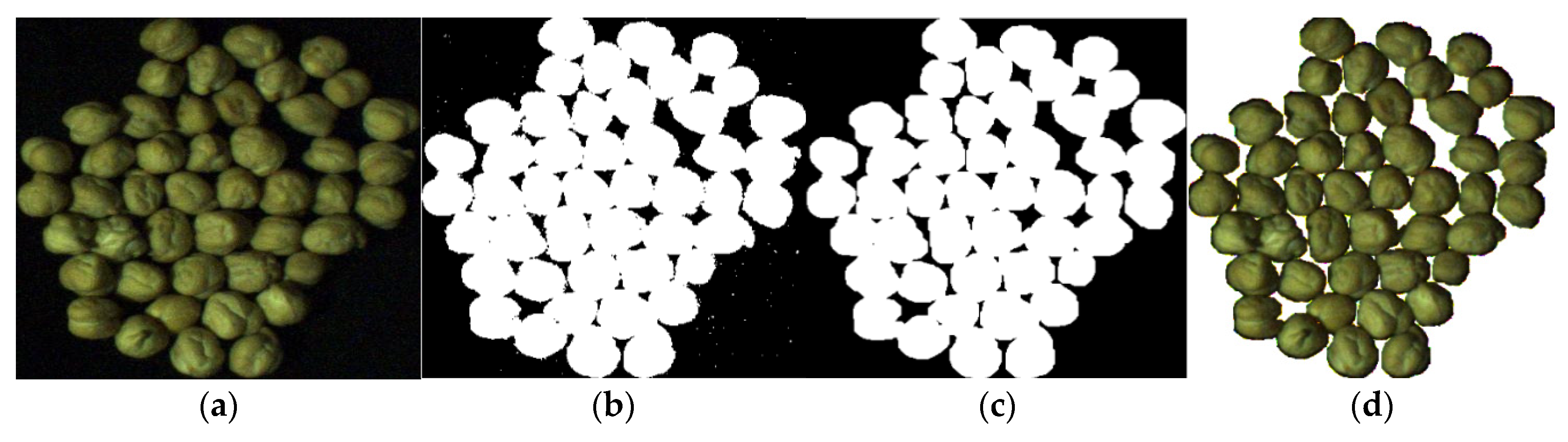
The division factor applied for segmentation turned out to be of great importance in the featureless method. A well-chosen factor with the proper level of tolerated black percentage proved to have a significant impact on the final accuracy of the classifier.

Nonetheless, there are a few weaknesses associated with these methods. The feature-based method with hybrid ANN-PSO relies on statistical inferences based on a small group of features, which could be insufficient for less-controlled conditions. Regarding the featureless method with three-layered backpropagation ANN, it is fed exclusively by color pixels. While the available chickpeas can actually be distinguished by color, this method requires working with a data set where all the images have been taken on the same conditions in order to ensure color constancy. Some factors such as lighting color, white balance of the camera, brightness or other external conditions, could result in changes in the observed colors. In that case, grayscale images should be used to achieve a higher robustness.

Further studies could take these issues into account in order to make the predictive potential of the classifier independent from the conditions under which the images were obtained. Convolutional neural networks (CNN) and deep learning could be a recommended way to achieve this goal. For this purpose, a larger dataset of images taken under more varied conditions would be necessary.

References

1. Eitzinger, A.; Cock, J.; Atzmanstorfer, K.; Binder, C.R.; Läderach, P.; Bonilla-Findji, O.; Bartling, M.; Mwongera, C.; Zurita, L.; Jarvis, A. GeoFarmer: A monitoring and feedback system for agricultural development projects. Comput. Electron. Agric. 2019, 158, 109–121. [Google Scholar] [CrossRef] [PubMed]
2. Díaz, O.; Ferreiro, T.; Rodríguez-Otero, J.L.; Cobos, Á. Characterization of chickpea (Cicer arietinum L.) flour films: Effects of pH and plasticizer concentration. Int. J. Mol. Sci. 2019, 20, 1246. [Google Scholar] [CrossRef] [PubMed]
3. Mpai, T.; Maseko, S.T. Possible benefits and challenges associated with production of chickpea in inland South Africa. Acta Agric. Scand. Sect. B Soil Plant Sci. 2018, 68, 479–488. [Google Scholar] [CrossRef]
4. Varshney, R.K.; Song, C.; Saxena, R.K.; Azam, S.; Yu, S.; Sharpe, A.G.; Cannon, S.; Baek, J.; Rosen, B.D.; Tar’an, B.; et al. Draft genome sequence of chickpea (Cicer arietinum) provides a resource for trait improvement. Nat. Biotechnol. 2013, 31, 240. [Google Scholar] [CrossRef]
5. Pandey, N.; Krishna, S.; Sharma, S. Automatic Seed Classification by Shape and Color Features using Machine Vision Technology. Int. J. Comput. Appl. Technol. Res. 2013, 2, 208–213. [Google Scholar] [CrossRef]
6. Kiratiratanapruk, K.; Sinthupinyo, W. Color and texture for corn seed classification by machine vision. In Proceedings of the 2011 International Symposium on Intelligent Signal Processing and Communications Systems: “The Decade of Intelligent and Green Signal Processing and Communications”, ISPACS 2011, Chiang Mai, Thailand, 7–9 December 2011. [Google Scholar]
7. Aygun, S.; Gunes, E.O. Computer vision techniques for automatic determination of yield effective bad condition storage effects on various agricultural seed types. In Proceedings of the 2016 5th International Conference on Agro-Geoinformatics, Agro-Geoinformatics 2016, Tianjin, China, 18–20 July 2016. [Google Scholar]
8. Hong, P.T.T.; Hai, T.T.T.; Lan, L.T.; Hoang, V.T.; Hai, V.; Nguyen, T.T. Comparative Study on Vision Based Rice Seed Varieties Identification. In Proceedings of the Proceedings—2015 IEEE International Conference on Knowledge and Systems Engineering, KSE 2015, Ho Chi Minh City, Vietnam, 8–10 October 2015. [Google Scholar]
9. Chaugule, A.; Mali, S.N. Evaluation of Texture and Shape Features for Classification of Four Paddy Varieties. J. Eng. 2014, 2014, 617263. [Google Scholar] [CrossRef]
10. Hernández-Hernández, J.L.; Ruiz-Hernández, J.; García-Mateos, G.; González-Esquiva, J.M.; Ruiz-Canales, A.; Molina-Martínez, J.M. A new portable application for automatic segmentation of plants in agriculture. Agric. Water Manag. 2017, 183, 146–157. [Google Scholar] [CrossRef]
11. Escarabajal-Henarejos, D.; Molina-Martínez, J.M.; Fernández-Pacheco, D.G.; Cavas-Martínez, F.; García-Mateos, G. Digital photography applied to irrigation management of Little Gem lettuce. Agric. Water Manag. 2015, 151, 148–157. [Google Scholar] [CrossRef]
12. Sau, S.; Ucchesu, M.; D’hallewin, G.; Bacchetta, G. Potential use of seed morpho-colourimetric analysis for Sardinian apple cultivar characterisation. Comput. Electron. Agric. 2019, 162, 373–379. [Google Scholar] [CrossRef]
13. Aznan, A.A.; Rukunudin, I.H.; Shakaff, A.Y.M.; Ruslan, R.; Zakaria, A.; Saad, F.S.A. The use of machine vision technique to classify cultivated rice seed variety and weedy rice seed variants for the seed industry. Int. Food Res. J. 2016, 23, S31. [Google Scholar]
14. Zhang, Y.; Wang, S.; Ji, G.; Phillips, P. Fruit classification using computer vision and feedforward neural network. J. Food Eng. 2014, 143, 167–177. [Google Scholar] [CrossRef]
15. HemaChitra, H.S.; Suguna, S. Optimized feature extraction and classification technique for indian pulse seed recognition. Int. J. Comput. Eng. Appl. 2018, XII, 421–427. [Google Scholar]
16. Li, X.; Dai, B.; Sun, H.; Li, W. Corn classification system based on computer vision. Symmetry 2019, 11, 591. [Google Scholar] [CrossRef]
17. Rumelhart, D.E.; Hinton, G.E.; Williams, R.J. Learning representations by back-propagating errors. Nature 1986, 5, 1. [Google Scholar] [CrossRef]
18. Hernández-Hernández, J.L.; García-Mateos, G.; González-Esquiva, J.M.; Escarabajal-Henarejos, D.; Ruiz-Canales, A.; Molina-Martínez, J.M. Optimal color space selection method for plant/soil segmentation in agriculture. Comput. Electron. Agric. 2016, 122, 124–132. [Google Scholar] [CrossRef]
19. Woebbecke, D.M.; Meyer, G.E.; Von Bargen, K.; Mortensen, D.A. Color indices for weed identification under various soil, residue, and lighting conditions. Trans. ASAE 1995, 38, 259–269. [Google Scholar] [CrossRef]
20. Meyer, G.E.; Mehta, T.; Kocher, M.; Mortensen, D.A.; Samal, A. Textural imaging and discriminant analysis for distinguishing weeds for spot spraying. Trans. ASAE 1998, 41, 1189. [Google Scholar] [CrossRef]
21. Golzarian, M.R.; Frick, R.A. Classification of images of wheat, ryegrass and brome grass species at early growth stages using principal component analysis. Plant Methods 2011, 7, 28. [Google Scholar] [CrossRef]
22. Meyer, G.E.; Neto, J.C. Verification of color vegetation indices for automated crop imaging applications. Comput. Electron. Agric. 2008, 63, 282–293. [Google Scholar] [CrossRef]
23. Kataoka, T.; Kaneko, T.; Okamoto, H.; Hata, S. Crop growth estimation system using machine vision. In Proceedings of the IEEE/ASME International Conference on Advanced Intelligent Mechatronics, AIM, Kobe, Japan, 20–24 July 2003. [Google Scholar]
24. Woebbecke, D.M.; Meyer, G.E.; Von Bargen, K.; Mortensen, D.A. Plant species identification, size, and enumeration using machine vision techniques on near-binary images. Opt. Agric. For. 1993, 1836, 208–220. [Google Scholar]
25. Kennedy, J.; Eberhart, R. Particle Sawrm Optimization. In Proceedings of the Neural Networks Proceedings IEEE International Conference, Perth, Western Australia, 27 November–1 December 1995. [Google Scholar]
26. Sabzi, S.; Abbaspour-Gilandeh, Y.; García-Mateos, G. A fast and accurate expert system for weed identification in potato crops using metaheuristic algorithms. Comput. Ind. 2018, 98, 80–89. [Google Scholar] [CrossRef]
27. Rasmussen, C.E. Fmincg Minimization Function. Available online: http://learning.eng.cam.ac.uk/carl/code/minimize/ (accessed on 22 October 2019).
28. Yuan, G.; Wei, Z.; Li, G. A modified Polak-Ribière-Polyak conjugate gradient algorithm for nonsmooth convex programs. J. Comput. Appl. Math. 2014, 255, 86–96. [Google Scholar] [CrossRef]
29. Nguyen, D.; Widrow, B. Improving the learning speed of 2-layer neural networks by choosing initial values of the adaptive weights. In Proceedings of the 1990 IJCNN International Joint Conference on Neural Networks, San Diego, CA, USA, 17–21 June 1990. [Google Scholar]
Figure 1. Sample images from each chickpea (Cicer arietinum L) variety: (a) Adel; (b) Arman; (c) Azad; (d) Bevanij; (e) Hashem.
Agronomy 09 00672 g001
Figure 2. Different stages of the segmentation process. (a) input image; (b) binary image after application of Equation (1); (c) result of morphology operator open; (d) resulting segmented image.
Agronomy 09 00672 g002
Figure 3. A random selection of 100 image patches with a division factor of 10. The size of each patch is 30 × 30 pixels.
Agronomy 09 00672 g003
Figure 4. Representation of a random selection of 100 sub-images associated to the hidden layer of the ANN obtained in the second method. Each 30 × 30 patch corresponds to the weights of a hidden neuron represented in RGB values.
Agronomy 09 00672 g004