Distributed Localization with Complemented RSS and AOA Measurements: Theory and Methods
by
 , , and
Slavisa Tomic
1,*,† ,
,
Marko Beko
1,2,† ,
,
Luís M. Camarinha-Matos
2,3,† and
Luís Bica Oliveira
2,3,† 1
COPELABS, Universidade Lusófona de Humanidades e Tecnologias, Campo Grande 376, 1749-024 Lisboa, Portugal
2
CTS/UNINOVA, Monte de Caparica, 2829-516 Caparica, Portugal
3
Faculty of Sciences and Technology, NOVA University of Lisbon, 2825-149 Caparica, Portugal
*
Author to whom correspondence should be addressed.
†
These authors contributed equally to this work.
Appl. Sci. 2020, 10(1), 272; https://0-doi-org.brum.beds.ac.uk/10.3390/app10010272
Submission received: 17 November 2019
/
Revised: 22 December 2019
/
Accepted: 24 December 2019
/
Published: 30 December 2019
(This article belongs to the Special Issue Multi-Channel and Multi-Agent Signal Processing)
Abstract
:Remarkable progress in radio frequency and micro-electro-mechanical systems integrated circuit design over the last two decades has enabled the use of wireless sensor networks with thousands of nodes. It is foreseen that the fifth generation of networks will provide significantly higher bandwidth and faster data rates with potential for interconnecting myriads of heterogeneous devices (sensors, agents, users, machines, and vehicles) into a single network (of nodes), under the notion of Internet of Things. The ability to accurately determine the physical location of each node (stationary or moving) will permit rapid development of new services and enhancement of the entire system. In outdoor environments, this could be achieved by employing global navigation satellite system (GNSS) which offers a worldwide service coverage with good accuracy. However, installing a GNSS receiver on each device in a network with thousands of nodes would be very expensive in addition to energy constraints. Besides, in indoor or obstructed environments (e.g., dense urban areas, forests, and canyons) the functionality of GNSS is limited to non-existing, and alternative methods have to be adopted. Many of the existing alternative solutions are centralized, meaning that there is a sink in the network that gathers all information and executes all required computations. This approach quickly becomes cumbersome as the number of nodes in the network grows, creating bottle-necks near the sink and high computational burden. Therefore, more effective approaches are needed. As such, this work presents a survey (from a signal processing perspective) of existing distributed solutions, amalgamating two radio measurements, received signal strength (RSS) and angle of arrival (AOA), which seem to have a promising partnership. The present article illustrates the theory and offers an overview of existing RSS-AOA distributed solutions, as well as their analysis from both localization accuracy and computational complexity points of view. Finally, the article identifies potential directions for future research.
1. Introduction
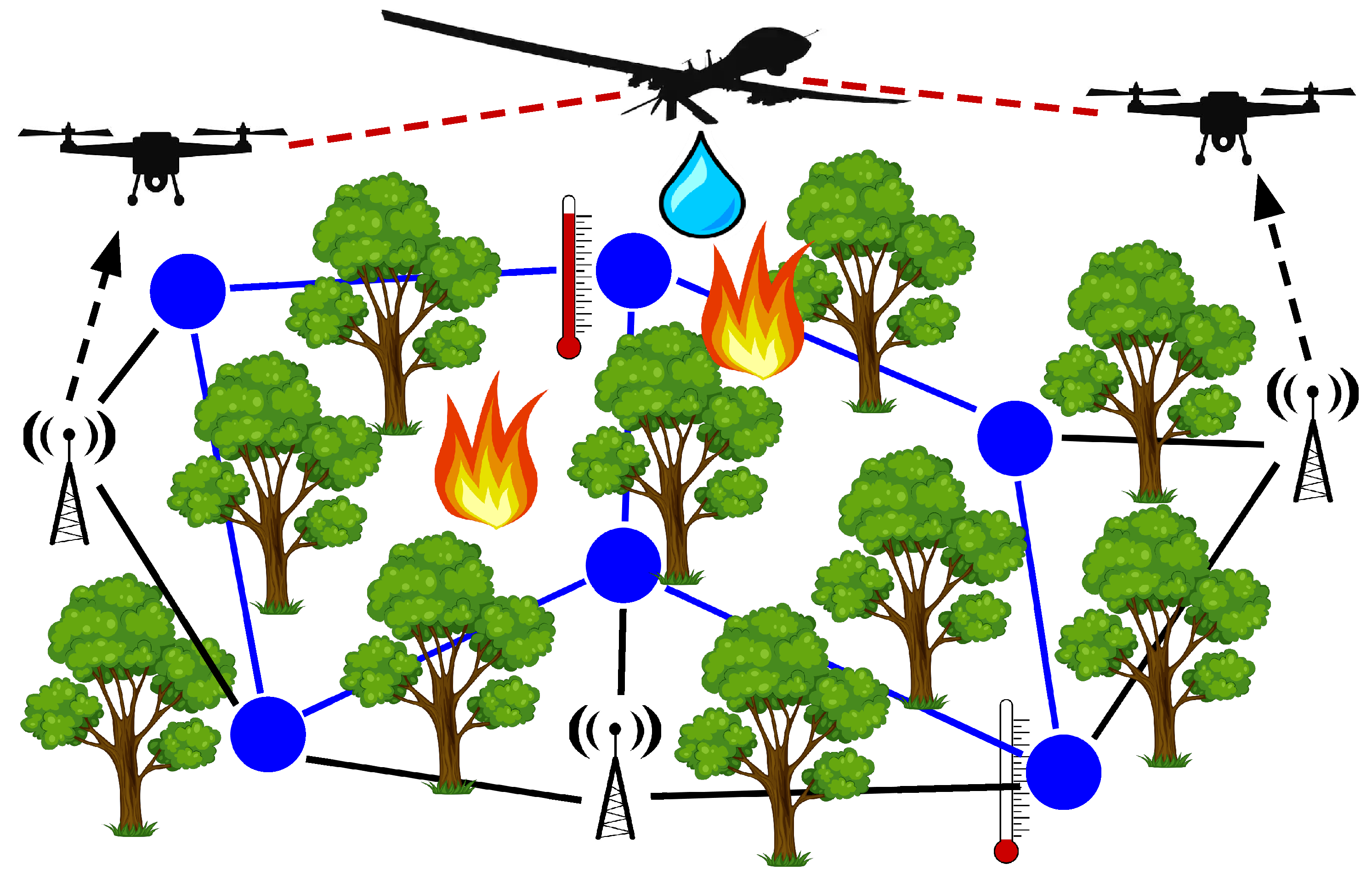
Real-time localization systems have gained much attention in the research community in the past several years [1,2,3,4,5,6,7,8,9,10,11,12,13,14,15,16,17,18,19,20,21]. In addition, works that highlight the potential of exploiting mobility of nodes in the localization process have emerged recently [22,23,24,25]. This is mainly owed to extensive technological advances and the requirement for seamless solutions in location-based services. It is expected that fifth generation (5G) network will have the potential to interconnect an extensive number of heterogeneous (mobile or stationary) devices (objects, users, vehicles) into a single network (of nodes), called Internet of things (IoT) [26]. In large-scale networks with thousands of nodes, human moderation is almost impossible, and autonomous network configuration becomes a very desirable feature. Therefore, the topic of localization is expected to attract even more interest in the future [27,28,29]. In fact, location-awareness is the key component in various other applications, such as emergency and health care services, intruder detection, precision agriculture, ocean data acquisition, or asset tracking, to name a few. For instance, location information is crucial for detecting and preventing fire hazards in forests, as illustrated in Figure 1, where a sensor network is employed to detect fire and, in cooperation with a fleet of autonomous aircraft, extinguish the danger [30].
A possible way to obtain a more accurate and granular information from the field is to employ a low cost, power-efficient, flexible, reconfigurable, and multifunctional smart sensing system (e.g., with programmable filters and power management units [31] or sensor-to-digital interface [32]). Such a system combines fixed and mobile sensors in a flexible wireless sensor network, which can acquire weather data, together with visible and infrared images for local classification of the fire front. These sensors could be installed on vehicles/aircraft involved in fire suppression, to reduce subjectivity of human-dependent analysis and improve operational coordination. This could be done by sending the location information of the target that sensed the fire danger (after processing it on its own) and fire intensity to the decision support systems to alert the system, in a similar manner as illustrated in Figure 1.
In terms of outdoor environments, global navigation satellite system (GNSS) is considered to be a universally accepted solution, since it offers global coverage and excellent localization accuracy. Nonetheless, its service is limited or even unavailable in indoor or obstructed environments where line of sight to satellites is obstructed, such as dense urban areas, forests, or canyons. Instead, alternative solutions for accurate localization based on already deployed terrestrial technologies is encouraged (which can possibly complement the ones based on satellites). Such technologies include wireless fidelity, Bluetooth, narrow-band IoT, ultra-wide band, near-field communication, radio-frequency identification, signals of opportunity, third generation partnership project/long-term evolution, and inertial measurement units. On the other hand, in indoor environments (or other ones where satellite reception is not feasible), there is no convergence towards a single solution, and it is an open question if there will ever be, due to the high degree of difficulty of the problem in such harsh environments (multipath propagation, obstruction of a direct path, etc.) [7].
In this survey, we study the problem of distributed localization based on an integration of a specific set of radio measurements. The problem is studied in detail from a signal processing point of view in its most general and widely used statistical form. A set of solutions to the problem, considered as the state-of-the-art, are presented and their main ideas are explained in a clear although informal fashion. The identified solutions are analyzed from both computational complexity and localization accuracy perspectives, with a theoretical lower bound included in the latter comparison in order to assess the margin available for further improvement. Lastly, we recognize some limitations of the existing solutions and identify possible directions for future research.
Throughout the survey, upper-case bold type, lower-case bold type and regular type are used for matrices, vectors, and scalars, respectively. is used to denote the n-dimensional real Euclidean space and the transpose operator is denoted by . The normal (Gaussian) distribution with mean and variance is denoted by , the von Mises distribution with mean and concentration parameter is denoted by , while the uniform distribution on the interval is denoted by . For any matrix , its trace is denoted by . The designation denotes a square diagonal matrix in which the elements of vector form the main diagonal of the matrix, and the elements outside the main diagonal are zero. The N-dimensional identity matrix is denoted by and the matrix of all zeros by (if no ambiguity can occur, subscripts are omitted). denotes the vector norm defined by , where is a column vector. For a matrix , denotes the -th entry of . The cardinality (the number of elements) of a set is denoted by and the statistical expectation of the argument as .
The remainder of this survey is organized as follows. In Section 2, we introduce the problem of distributed target localization in a generic framework, and we provide details about the main performance metrics often used in the literature. We also summarize the main sources of errors for the considered radio measurements. Section 3 presents a set of existing statistical-based estimators that are available to solve the considered problem. This section summarizes the main ideas behind each of the existing solutions, without a rigorous formal analysis. In Section 4, we offer a set of results in order to give an intuition to the reader about the performance of each of the existing solution from both computational complexity and localization accuracy points of view. Lastly, Section 5 concludes the survey and identifies possible future research directions regarding the problem of interest.
2. RSS-AOA Distributed Localization Problem
Future networks are expected to be composed of heterogeneous devices. Here, we use a generic term, nodes, to denote (any kind of) these devices. Note that wireless localization systems typically assume the presence of some reference nodes (usually called anchors or landmarks) deployed at fixed known locations (or equipped with GNSS receivers to determine their locations) and one or more nodes with a location one desires to determine (often referred to as targets or agents). Across the literature, the used terminology is not universal, and it frequently depends on the deployed technology. For instance, in cellular networks, the term base station is employed for anchors, whereas the term mobile station is utilized for a target node (the term user equipment is frequently used in the literature, as well) [33].
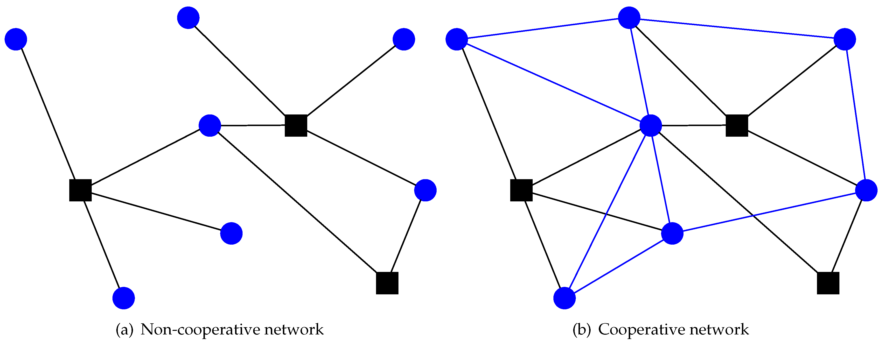
In general, the solution to localization problem comprises two phases: collecting measurements and exploiting them together with some known reference points to estimate target locations [34]. In the former phase, nodes communicate between themselves in order to acquire (radio) measurements. Based on the type of communication, we here distinguish two types of networks: non-cooperative (targets communicate with anchors exclusively) and cooperative (targets communicate with any nodes within their communication range), as illustrated in Figure 2. While in non-cooperative networks one takes advantage of known locations of anchors, which minimizes the error propagation due to localization inaccuracy, in many applications the number of anchors is scarce, and due to limited resources of nodes (e.g., battery life), only some of them can establish direct communication with anchors; hence, node cooperation is required in order to determine locations of all targets. It is well known that node cooperation can bring advantages and lead to better decisions, especially when connectivity in the network is limited [35,36,37].
The most frequent radio measurement techniques utilized in practice are time (difference) of arrival, round trip time, phase of arrival, received signal strength (RSS) and angle of arrival (AOA). Moreover, the notion of hybrid system in which two (or more) measurements are integrated has gained much popularity lately [4,7,12,38]. Even though it is intuitive that more information should lead to better localization accuracy, one should note that joining any two measurements does not necessarily bring advantage in every scenario [12,39]. In the latter phase, the measured quantities are converted into distance or direction estimates, which combined with some known reference locations are processed to determine locations of interest.
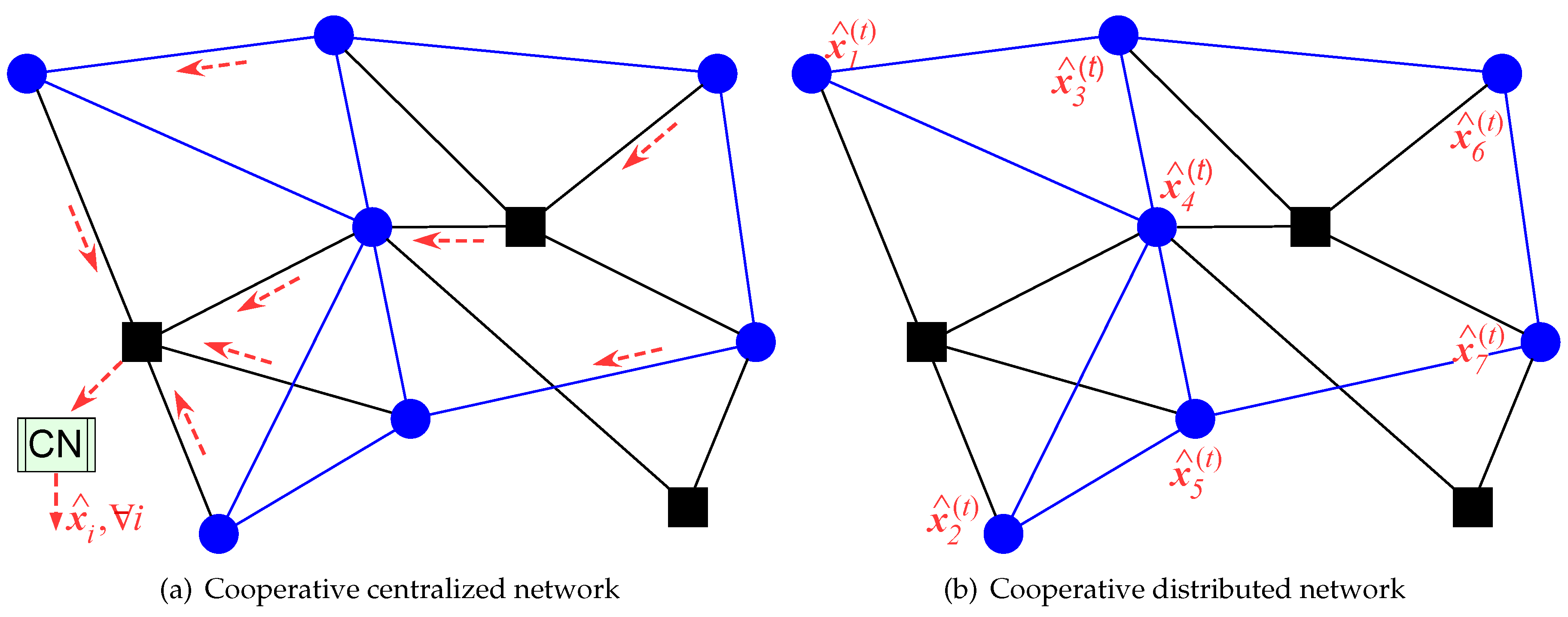
Depending on where the information processing is occurring, we discern two types of networks: centralized (assumes existence of a sink or a central node (CN) in the network which collects all measurements gathered in the network and executes all information processing) and decentralized or distributed (each target node collects measurements from its direct neighbors and executes all information processing by itself, usually in an iterative fashion), as illustrated in Figure 3. Both types of networks have their pros and cons: the centralized ones are more stable, but their computational burden becomes too costly as the number of nodes in the network increases, whereas the computational cost in distributed networks depends only on the size of local neighborhood of a target, but distributed processing often requires iterations which might disseminate localization errors across the entire network [40]. Here, we will concentrate on the distributed cooperative networks exclusively, both because in 5G networks we are expected to deal with networks with a large number of nodes, and because some of them might not wish to reveal their private content (e.g., their objective functions) to other nodes.
2.1. Problem Statement
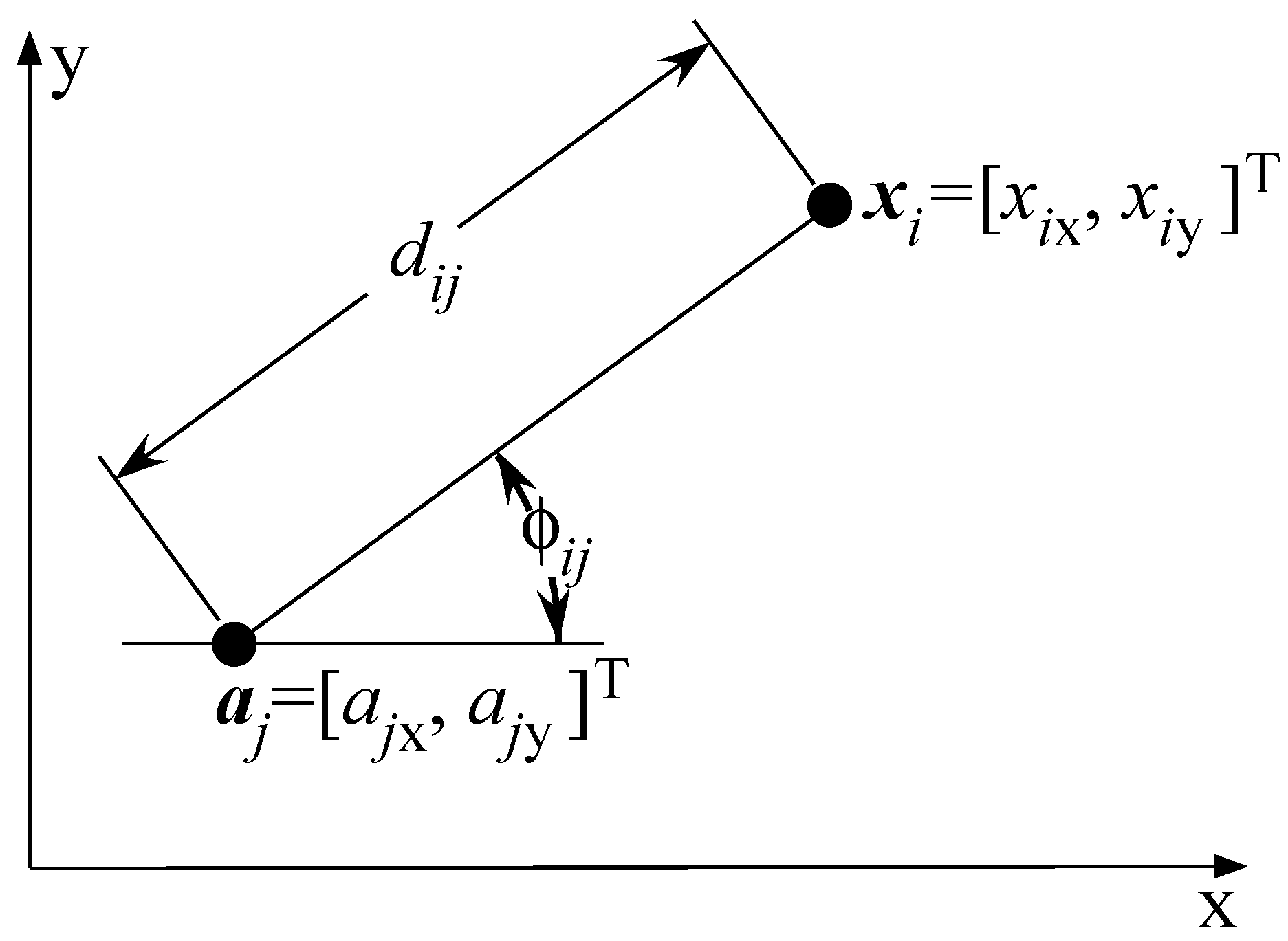
Let us consider a radio localization system consisting of nodes (M of which are targets and N anchors, with preferably ), where their true locations are denoted by , ... , and , , respectively, with or 3. One can view such a system as a connected graph , with vertices and a set of edges, . Thus, we can also define the set of all targets, , as well as the set of all anchors, , where it follows that . Due to limited energy constraints, it is assumed that nodes have constrained communication range. If two nodes, i and j, are within the communication range of each other, they can interact, i.e., there is an edge between them, , with , if the and , if the . Consequently, we can divide the set into two subsets, i.e., and . Lastly, let us define the neighborhood of the i-th target node as . The localization system of interest in a 2-dimensional space is illustrated in Figure 4, where the distance and direction information are extracted from RSS and AOA measurements, respectively.
RSS is defined as the voltage level measured by a receiver’s RSS indicator circuit. It is often equivalent to measured power, i.e., the squared magnitude of the signal strength. In free-space, signal power decays proportionally to , where d is the distance between a transmitter and a receiver. However, in practical applications the environment in which the signals propagate is not free-space, and an obstructed channel decays proportionally to instead, where is the path loss exponent (PLE) which indicates the rate at which the received strength decreases with distance [41]. Typically, the RSS sensed by the i-th node related to the transmission of the j-th node [42] (Ch. 3), [43,44], is defined as
where is the reference RSS measured at a short reference distance (), is the distance between nodes i and j, and is the log-normal shadowing term modeled as a zero-mean Gaussian random variable with variance . Without loss of generality, it is assumed here that RSS observations between target nodes are symmetric, i.e., .
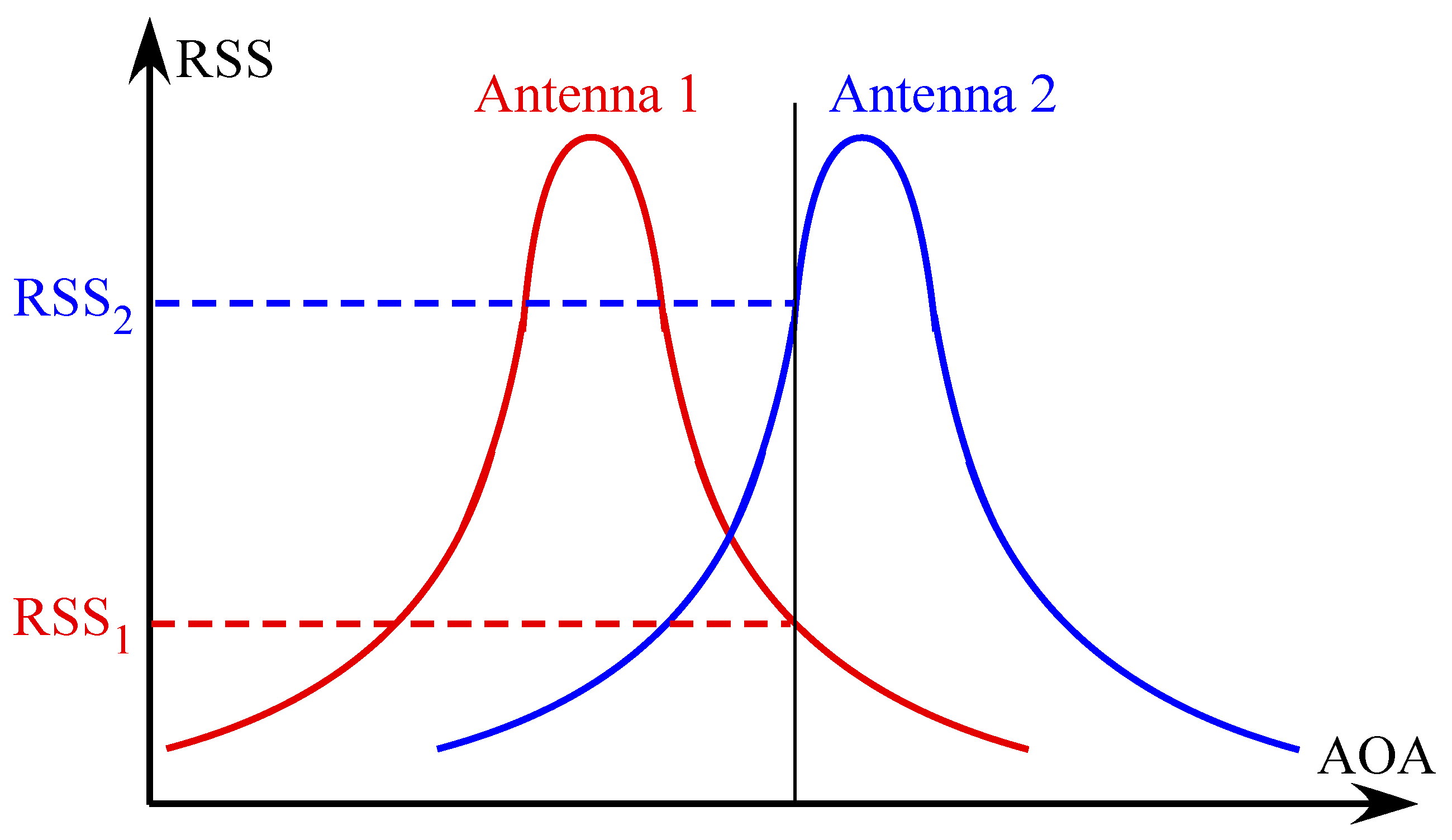
Two common ways to measure AOA are by employing antenna arrays and by using directional antennas. The former method is based on the so-called array signal processing techniques at sensor nodes. In this method, the AOA is estimated from the differences in the arrival times of a received signal at each of the array elements. The latter method estimates AOA based on the RSS ratio between two (or more) directional antennas installed on a node, as illustrated in Figure 5. Usually, two directional antennas are pointed in different directions so that their main beams overlap, and the overlap is used to estimate the AOA from the ratio of their individual RSS values [41]. The AOA can also be estimated from RSS measurements by employing electronically steerable parasitic array radiator antennas [45] or by rotating a directional antenna at the receiving end [46], or even by using video cameras [47]. It is also worth mentioning that some recent works estimate the angle by exploiting the known network topology, rather than installing any additional hardware at the receiving end [48]. Furthermore, phase of the received signal can play a significant role in the direction of arrival estimation [49,50].
From geometry, azimuth angle measurements (at anchor nodes) [15,46,51,52,53] can be modeled as
where and denote, respectively, the l-th coordinate of k-th target and anchor node, and is the measurement error of the azimuth angle, modeled as a zero-mean von Mises random variable with the concentration parameter , i.e., . The von Mises distribution can be seen as a circular analogue of the Normal distribution. There is a close connection between the mean direction and the concentration parameters of the von Mises distribution and the mean and variance of the Normal one [54,55].
In order to simplify the notation, we define , , , (), and . Following the model in (1), the conditional probability density function (PDF) of RSS measurements is given by
In a similar manner, according to the model in (2), the conditional PDF of AOA measurements can be written as
where is the modified Bessel function of first kind of order k [54,55], and is a unit vector.
If one would maximize (3),(4), one would obtain the maximum likelihood (ML) estimator [56] (Chapter 7) of . In distributed networks, the ML problem is actually split into M local ML estimators, which is then solved individually by each one of the target nodes, resorting only to measurements acquired from the target’s direct neighbors. Nonetheless, the ML estimator obviously implies dealing with highly non-convex problem, in which a closed-form solution is not directly attainable; hence, directly solving the RSS and AOA ML estimator might not be feasible in practice. Therefore, many researchers opt to tackle an approximation of the ML estimator instead.
2.2. Performance Metrics
In general, requirements and performance metrics depend on the application for which an estimator will be employed. In practice, some intrinsic uncertainties are always present in the system (such as measurement noise), which naturally lead to errors in the node’s location estimate. The location error of the i-th node is defined as , where is the estimated location of the true node’s location, . One can use this error to build a variety of statistics that can be utilized as performance metrics. One of the most popular in the localization literature is the root mean square error (RMSE), given by
However, in practical performance evaluation tests, the expectation is approximated by a set of Monte Carlo () trials. In addition, due to the consideration of M target nodes in the network, one can actually define the average RMSE (ARMSE) as
where represents the estimate of the true j-th target location, , in the i-th Monte Carlo run. ARMSE can be thought of as accuracy, since it is the rate of the statistical deviation of the location estimate from its real location.
In order to get a notion of how good the performance of an estimator actually is, it is useful to compare it against some benchmark. Theoretically, the best achievable performance is often bench-marked by the Cramér-Rao lower bound (CRLB) [56] (Chapter 3). If one defines the co-variance matrix of an estimator, where the estimate is denoted by, for instance , with
then we know that the covariance is bounded by
where represents the Fisher information matrix (FIM) and means that the matrix is non-negative definite. The interested reader can find the derivation of the CRLB for the considered localization problem in the Appendix A.
The reason why ARMSE is the most widely used performance metric in the localization literature is the fact that it is the best finite-sample approximation of the standard error, which is usually the most desired optimality criterion in terms of errors. Obviously, the ARMSE might not capture completely the accuracy of an estimator, and one may opt to employ other performance metrics. These include localization error outage, cumulative distribution function of the localization error, average Euclidean error, geometric average error, etc. [57,58].
It should be noted that performance evaluation is never completely fair nor impartial. To some extent, this is owed to the fact that elementary metrics are not able to capture a complete picture of an estimator, while those that are more complete are too complex and are often biased due to subjective interpretations (for instance, a metric can be in favor of an estimator that implicitly tries to optimize this same metric) [57]. To prevent such issues, in general, one should choose a metric that is the most relevant for the intended application.
2.3. Main Sources of Errors
All terrestrial localization systems based on pair-wise measurements closely rely on the quality of the measurements. Therefore, the key objective in establishing reliable localization systems is to accurately model the main degrading effects of the channel through which the radio signals propagate. In many practical applications, the environment in which the propagation of the radio signals occurs consists of various stationary or mobile objects/people (obstructions) that impede line of sight between the transmitter and the receiver, and cause reflections of the signal. These factors severely aggravate the task of propagation modeling [41].
In general, range and direction measurements involved in the process of localization are affected by both time-varying errors and static, environment-dependent errors [59]. The former ones might occur due to additive noise and interference, and can be alleviated by averaging over several measurements in time. The latter ones are the product of physical arrangement of objects (such as walls and furniture) in a given surrounding in which the network is operating. Owing to unpredictability of the surrounding, both types of errors are unmanageable and are treated as random. Nevertheless, in a given environment in which objects are mostly stationary, environment-dependent errors will be largely constant over time.
In practice, multipath signals and shadowing are the main causes of errors in RSS measurements [42,60]. The former sources of error occurs because of reflections, causing multiple copies of the signal (of various amplitudes and phases) to arrive at the receiving end. These signals can cause destructive and constructive interference, which might result in weak correlation of RSS with distance. The latter source of error are environment-dependent and are caused by attenuation of the received signal due to obstructions, since the signal penetrates or diffracts around. This type of errors are often referred to as medium-scale fading.
Similar with RSS measurements, the main source of errors in AOA measurements is the multipath, although additive noise can also cause inaccuracies [41]. Essentially, at the receiving end, we desire to determine the direction of arrival of the signal coming from a direct path from the transmitting end. This can be challenging to achieve in multipath channels, since instead of finding the highest peak of the cross correlation, the receiver has to determine the first-arriving peak, because there is no guarantee that the direct-path signal will be the strongest of the arriving signals. Many multipath signals arrive instants after the direct-path signal, and they can obscure the location of the peak from the direct-path signal. Furthermore, in some cases the direct-path signal can be considerably attenuated compared with its late-arriving multipath components, which might cause the receiver to overlook it completely [41].
3. Existing Methods
In this section, we give a brief overview of the existing (state-of-the-art) distributed RSS-AOA localization algorithms, summarizing their main ideas without going into many technical details; we refer the interested reader to see all specific technical details in the respective works, cited below.
3.1. Second-Order Cone Programming (SOCP) Method
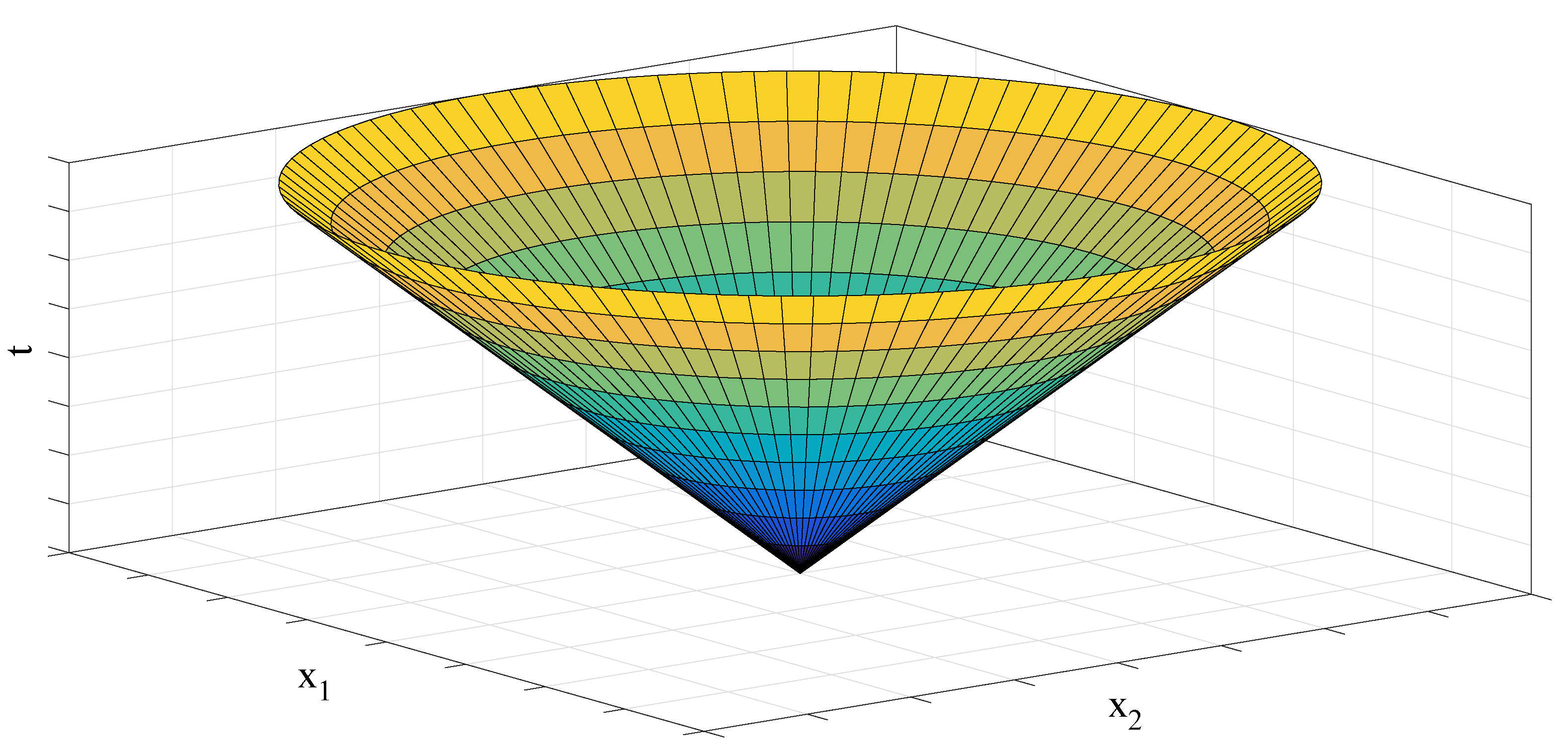
The authors in [61] studied the problem of distributed target localization based on integrating RSS (measured at all nodes) and AOA measurements (measured at anchor nodes exclusively) and proposed an algorithm based on convex optimization, namely SOCP. The main idea of the algorithm is based on deriving a relaxed version of the original problem by applying a sequence of second-order cone constraint relaxations of the form , where and is the optimization variable. This second order cone constraint is the same as requiring the affine function to lie in the second-order cone in [62], which is illustrated in Figure 6. Once the relaxed, convex, problem is derived, it can be readily solved by off-the-shelf solvers, such as CVX [63], a MATLAB software for disciplined convex programming. In [61], it was assumed that network coloring scheme [40] was achievable in order to establish a working hierarchy between targets and avoid message collisions.
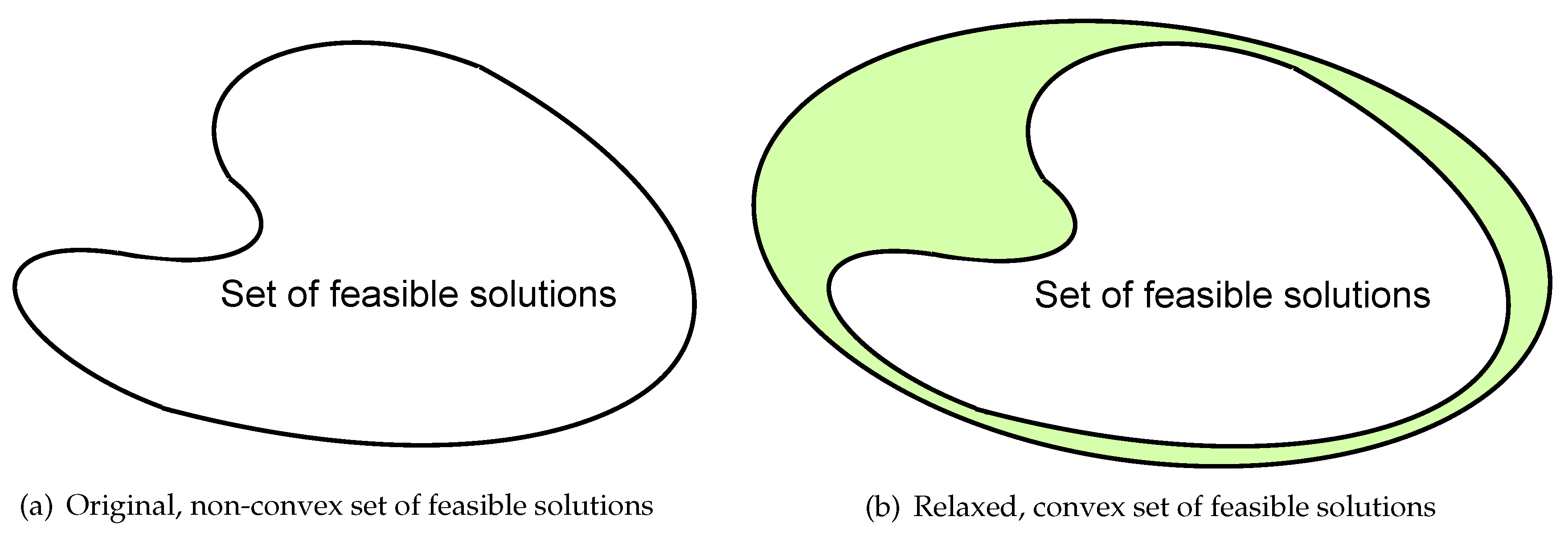
Although convex problems are easily solved Today, their solution is sub-optimal due to problem relaxation, which might increase the set of feasible solutions, as illustrated in Figure 7. Therefore, the quality of their solutions depends on the tightness of the applied relaxations since, otherwise, one may end up with a solution from the expanded set that might be considerably far away from the true one.
3.2. Linear Least Squares (LLS) Method
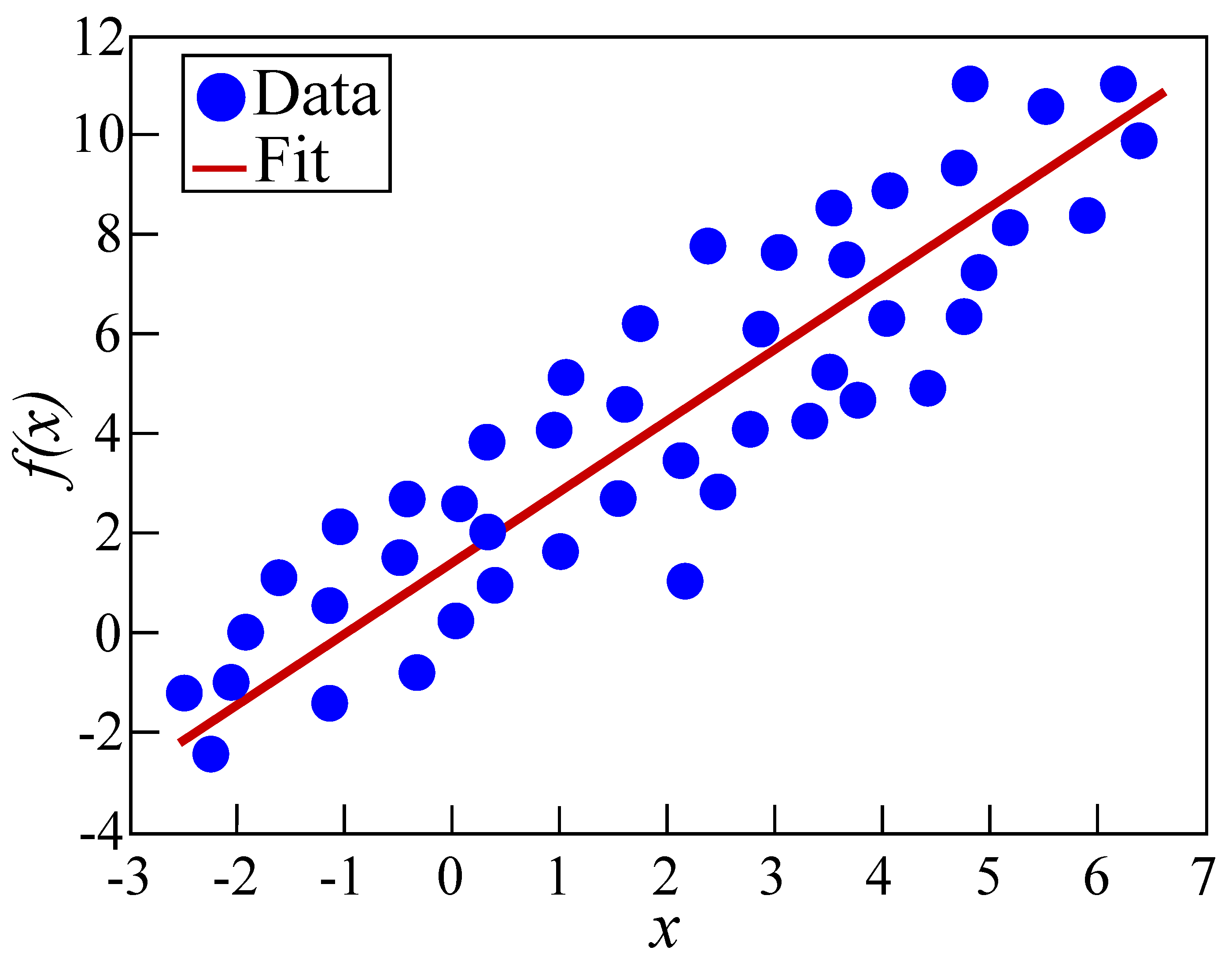
In [38], the authors considered the problem of distributed target localization based on fused RSS and AOA measurements, with the main difference (in comparison with the problem studied in [61]) that they assumed that all nodes in the network are capable of measuring both RSS and AOA quantities. The authors in [38] proposed an algorithm based on LLS approach. LLS is a special subclass of convex optimization, where the objective function is of the form , and the solution is given in closed form as . It is a standard approach in regression analysis, where the main idea is to give the best fit that minimizes the sum of squared residuals, where a residual is considered to be the difference between an observed value and the fitted one provided by the model, as illustrated in Figure 8. LLS requires the model to be linear, which is evidently not the case for RSS nor AOA. Nevertheless, rather than applying a sequence of approximations to the model, the authors in [38] cleverly took advantage of the geometry of the problem at hand. More precisely, for each of the anchors, they estimated the distance to a target of interest, and together with the measured AOA, obtained an estimate of the target location, much like the illustration shown in Figure 4. Of course, distance and angle estimates were employed, rather than their true values. It was considered that there exists some node synchronization protocol which allowed targets with direct edges to anchors to localize themselves first, after which they played a role of quasi-anchors (reference points with imperfectly known locations, also called helpers [64]) to help localize the targets with no direct link to anchors, iteratively.
3.3. MCMC-MH Method
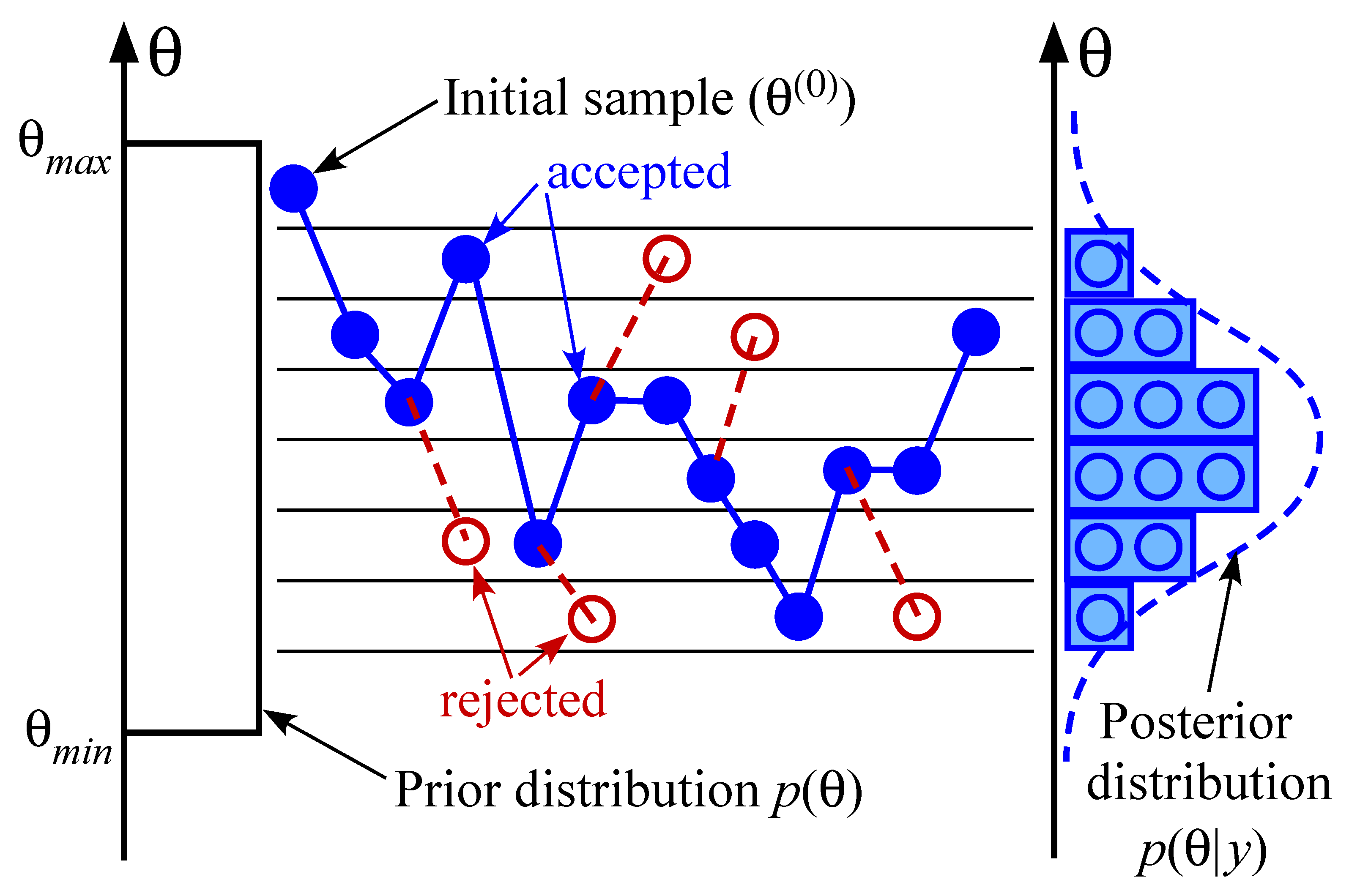
The authors in [65] proposed a different approach based on Bayesian regression. Their approach is known as Markov chain Monte Carlo with Metropolis-Hastings (MCMC-MH) algorithm [66] (Chapter 6), [67] (Chapter 12). In such an approach, one is interested in sampling from a generic distribution, i.e., from the posterior distribution of a parameter, say , given its prior and likelihood, i.e., . This approach is often used when one knows how to write , but does not know how to generate a random number from this distribution (because it is too complex). Hence, one generates a sequence of values in such a way that when , we have that . The samples can later be exploited to estimate, for instance, the mean of the posterior distribution.
To better explain the main idea of MCMC-MH, we divide it into three parts. In the first part, the term Monte Carlo refers to generation of random numbers from a chosen distribution, called the proposal distribution. The proposal distribution is entirely up to the user, but is usually chosen as a Normal one with predefined mean and variance. The key idea of Monte Carlo approach is that the more generations are performed, the more similar the resulting density is with the proposal density. In the second part, one has a Markov chain that is a sequence of numbers, where each number is dependent on the previous one in the sequence. If one generates a sequence of numbers using Markov chain Monte Carlo method, the trace plot of the parameter of interest, , is often called a random walk. Finally, the Metropolis-Hastings algorithm is used to determine which generated values of to accept/reject. It is based on the proportion between the posterior probability of a newly generated value and the posterior probability of the previously accepted value, i.e.,
One then calculates the acceptance probability of the new point as . Finally, to check whether to accept/reject the new value, one draws a uniform random number and keeps if the acceptance probability is greater then the uniform random number and rejects otherwise. A simplified pseudo-code of MCMC-MH algorithm is summarized in Algorithm 1 and is graphically illustrated in Figure 9.
| Algorithm 1 Summary of MCMC-MH algorithm |
|
3.4. Generalized Trust Region Sub-Problem (GTRS) Method
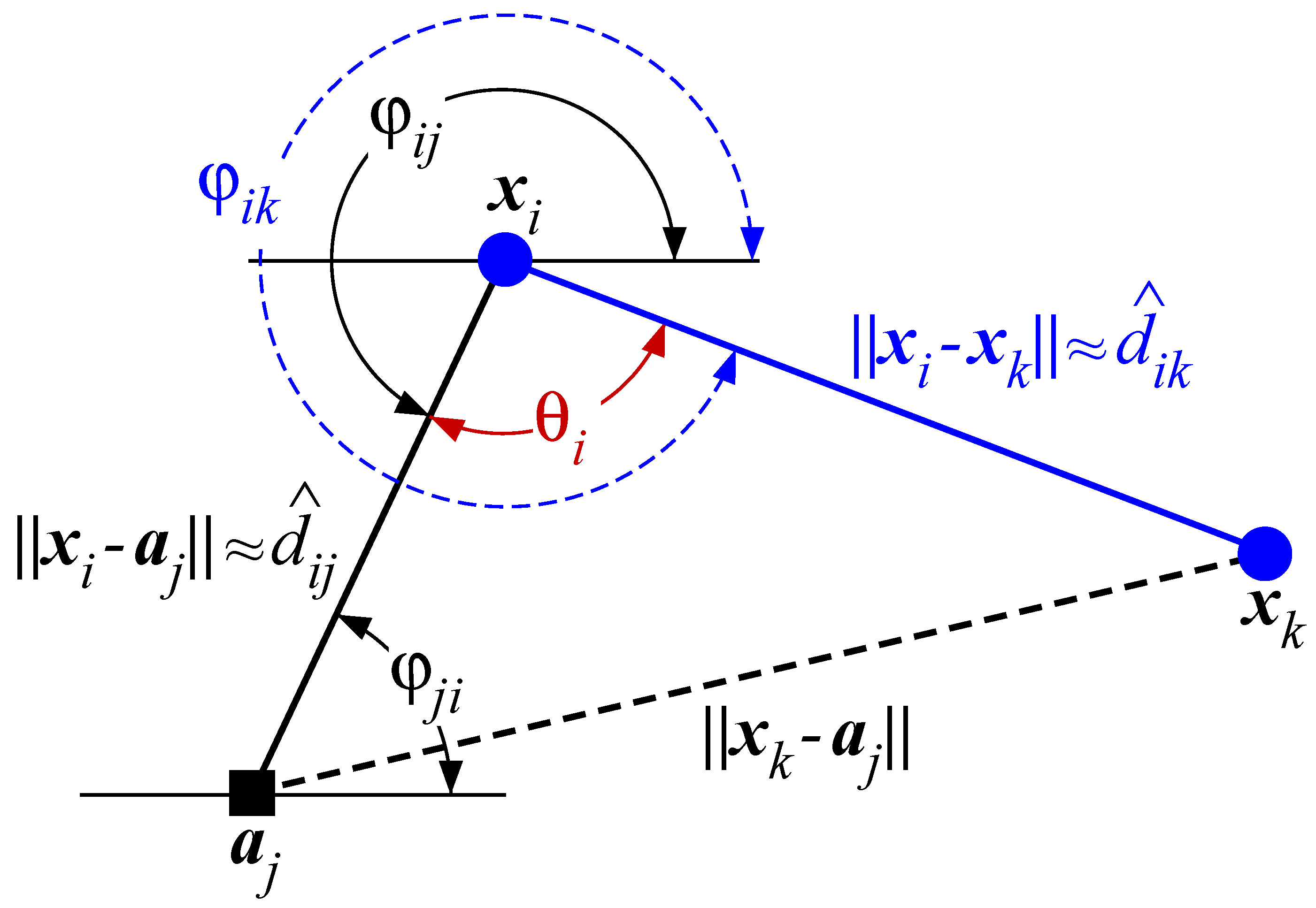
A geometric approach was presented in [68], where the authors considered that AOA measurements are acquired at anchor nodes, exclusively. They considered a multi-hop approach in order to form triangles in which a target node, , with a direct edge to an anchor node, , plays a role of a pivot and connects its target neighbor, , to the anchor, as illustrated in Figure 10.
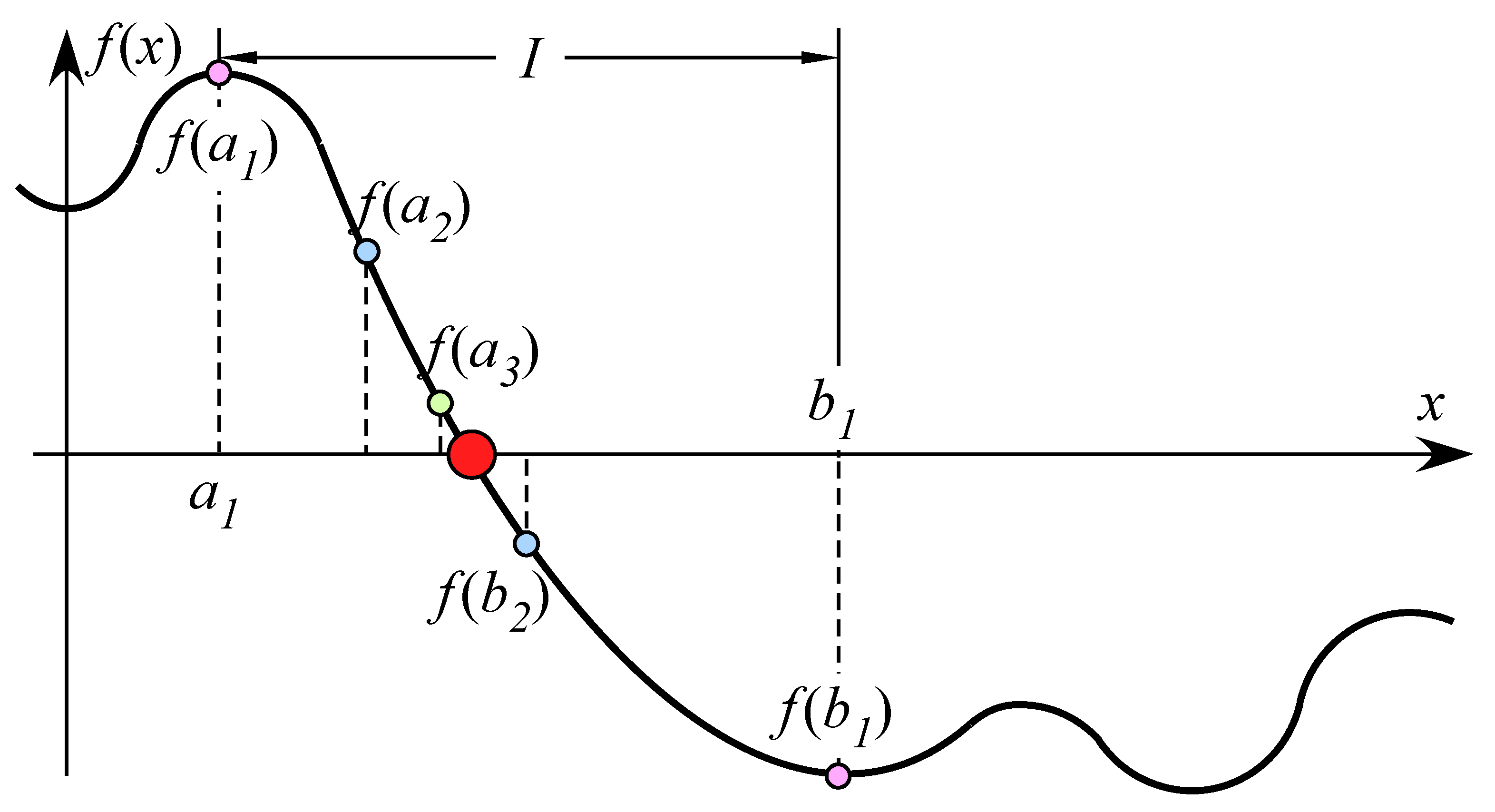
The procedure proposed in [68] can be explained in three steps. Firstly, all target nodes with direct edges towards anchor nodes are localized, by means of weighted central mass (WCM). In the second step, the localized target nodes were considered as quasi-anchors in order to localize the remaining target nodes. This was done by taking advantage of the network geometry in the formed triangles and applying the law of cosines, which led to straightforward formulation of the problem in a GTRS framework [69,70]. This type of problems has a very convenient characteristic, which is that, even though non-convex in general, one can determine an interval I on which the function is monotonically decreasing [69]. Therefore, GTRS can be efficiently solved by merely a bisection procedure, as illustrated in Figure 11. Finally, in the last step of the algorithm, the authors performed a refinement step based on WCM, in which they exploited the estimated locations of the target nodes in the previous steps and the acquired angle and distance measurements/estimates.
An overview of the main characteristics of all described algorithms is given in Table 1, where the notations “noise STD” and “” are used to denote the noise standard deviation and node’s transmit power. Table 1 shows that all considered algorithms require that all nodes measure the RSS quantity, while some of the algorithms require that only anchor nodes measure the AOA quantity. It can also be seen from the table that SOCP is perhaps the most universal approach in terms of applicability, since it can be used for both cases of known and unknown , and does not require knowledge about noise STD. The remaining methods (at least in their original form) are only suitable for the case where is assumed known. Furthermore, some of them require knowledge about the noise STD, which might jeopardize their localization accuracy in the case where this information is not perfectly known, as it will be shown in the following section.
4. Performance Analysis
This section offers a set of numerical results with the objective to give the reader a better understanding of the performance of the considered approaches. The performance is analyzed from both computational complexity and localization accuracy point of view. Moreover, the results for average execution time of the algorithms are also included.
4.1. Analysis of Computational Complexity
Here, we analyze the worst-case computational complexity of an algorithm. This is achieved by considering a fully connected network (i.e., the total number of neighbors of each target is assumed to be ). In addition, the computational complexity of each algorithm is expressed as a function of the dominating terms (the smaller terms are disregarded), written as a function of . The results of the considered algorithms are given in Table 2, where , , and are used to denote the maximum number of steps allowed in the bisection procedure in [68], the number of generated candidates and the number of iterations in [65], respectively. Furthermore, we also present the execution time of the considered algorithms, which is calculated as an average execution time per target to localize itself in the scenario where , , m in runs. The simulations were performed on the Intel(R)Core(TM) i7-4710HQ CPU with 2.50 GHz and 16 GB RAM.
One can see from Table 2 that the computational complexity of distributed algorithms depends mainly of the size of local neighborhood of a target, rather than on the size of the whole network (which is a characteristic of centralized ones). Furthermore, Table 2 exhibits that computational complexities of the SOCP approach in [61] and the MCMC-MH approach in [65] are the most burdensome ones. Although the complexity of MCMC-MH is actually linear in , its execution time is higher by far than those of LLS and GTRS, and even that of SOCP. This can be explained by the fact that a high number of candidates is generated and evaluated in every step of MCMC-MH procedure, which even though not especially intensive in terms of computational cost, is very time-consuming as the number of candidates increases. Finally, one can see that LLS and GTRS approaches have linear computational complexity in and their time execution confirms that they might be suitable for real-time implementation, despite the fact that GTRS requires some iterations in the bisection procedure to reach its final solution.
4.2. Analysis of Localization Accuracy
In this section, a set of simulation results are presented in order to evaluate the performance of the existing algorithms in terms of localization accuracy. In the simulations presented here, all nodes were deployed completely randomly inside a square area with edge length m in each Monte Carlo () run, forming connected networks. RSS and AOA measurements were generated according to (1) and (2). The reference distance was set to m, the reference RSS to dBm, and the PLE to . The maximum number of steps in the bisection procedure was set to . Moreover, dB and were adopted, where the latter parameter corresponds to the Normal standard deviation of deg, since [54,55].
In this analysis, the following assumptions are made about the network:
- (1)
- The network is connected and does not vary during the computational period;
- (2)
- All nodes are suitably equipped to measure RSS of the received radio signal;
- (3)
- Some nodes (anchors) or possibly all of them are conveniently equipped to measure AOA of the received radio signal;
- (4)
- Working order of the nodes is synchronized.
The first part of Assumption (1) guarantees that there is a path between nodes i and j, , while the second part ensures that there is no topology variation (node/edge failure, node/edge addition or node movement) during the time required for information processing. Assumptions (2) and (3) are necessary in order for the nodes to acquire RSS and AOA measurements. While RSS measurements are cheap (because they do not require specialized hardware) and are thus widely available Today in almost all devices, in order to measure AOA quantity, typically directional antennas, antenna arrays or video cameras are required at the receiving end. Assumption (4) is made for the sake of simplicity, since node synchronization is a difficult problem to tackle in distributed networks, and it does not represent the main concern of this work. One possible way to achieve node synchronization could be by using network coloring scheme, as explained in [40,71,72], or any other medium access protocol.
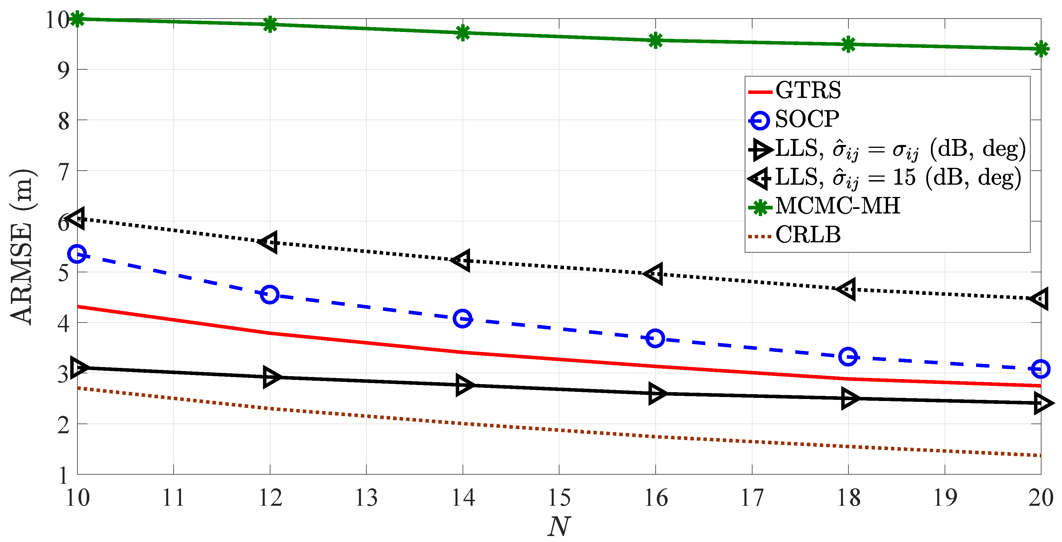
Figure 12 depicts ARMSE (m) versus N comparison for fixed and m. It clearly shows that the performance of all methods improve as N grows. This behavior is anticipated, since the quantity of reliable information in the network increases when more anchor nodes are added into the network. The figure shows that the performance of LLS is the best one. This is not a surprise, since LLS assumes that all nodes can measure AOA and it assumes perfect knowledge about the noise powers, which might not be feasible in practical scenarios where only a single measurement between pair of nodes is used for localization. Hence, in order to study the robustness of this method to imperfect knowledge about the noise power, the results for LLS when instead of the true value of (dB, deg), (dB, deg) is used are also included. It can be seen that LLS is sensitive to imperfections about this information. Finally, Figure 12 shows that there is still considerable room for further improvements, since there is a margin between CRLB (assuming that all nodes can measure the AOA quantity) and the existing methods.
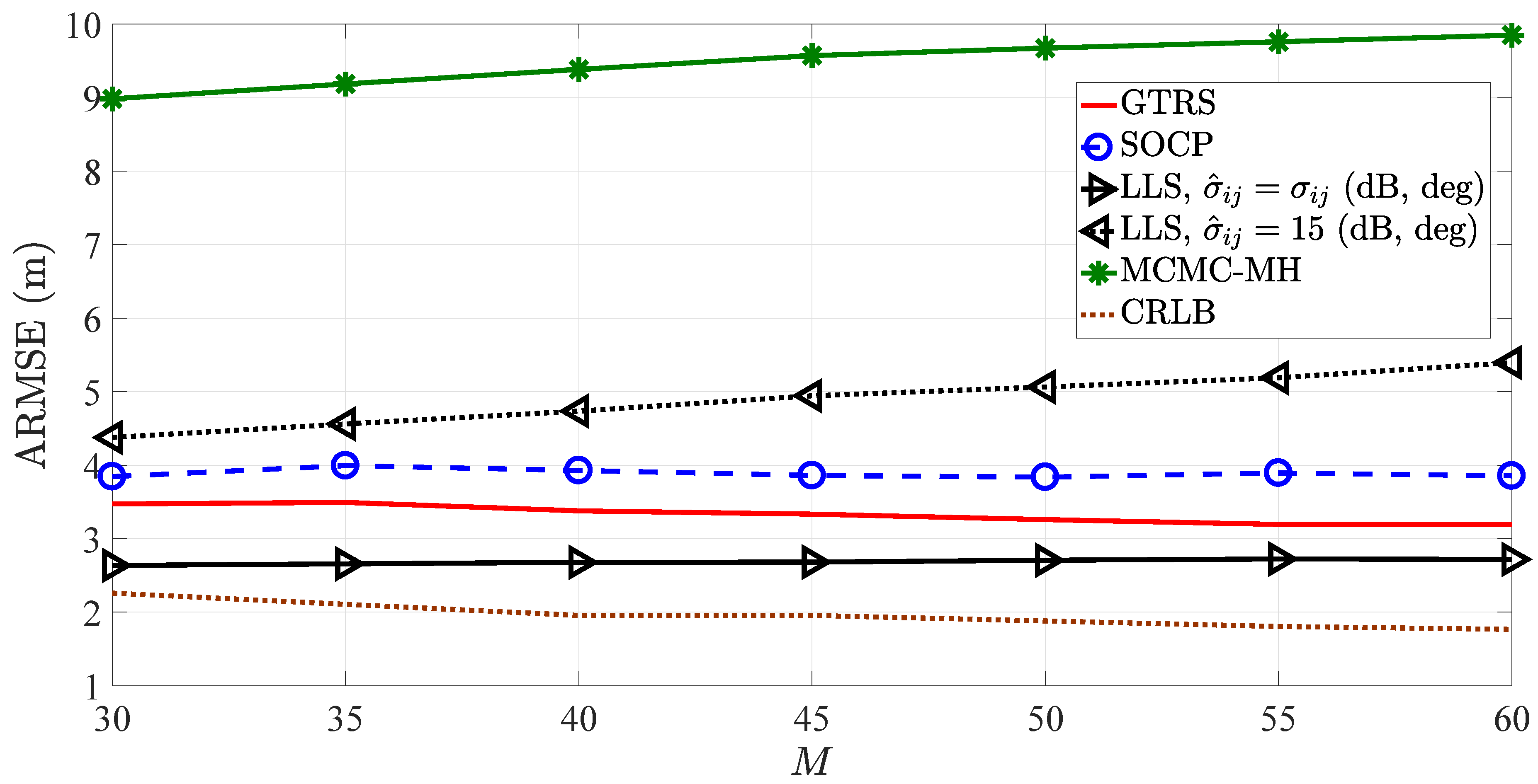
Figure 13 depicts ARMSE (m) versus M comparison for fixed and m. It can be seen that the performance of LLS and MCMC-MH deteriorates and the performance of SOCP and GTRS meliorates slightly as M increases. This indicates that the latter two methods benefit from additional node cooperation achieved by introducing more target nodes into the network, while the latter ones are unable to take advantage of this additional cooperation.
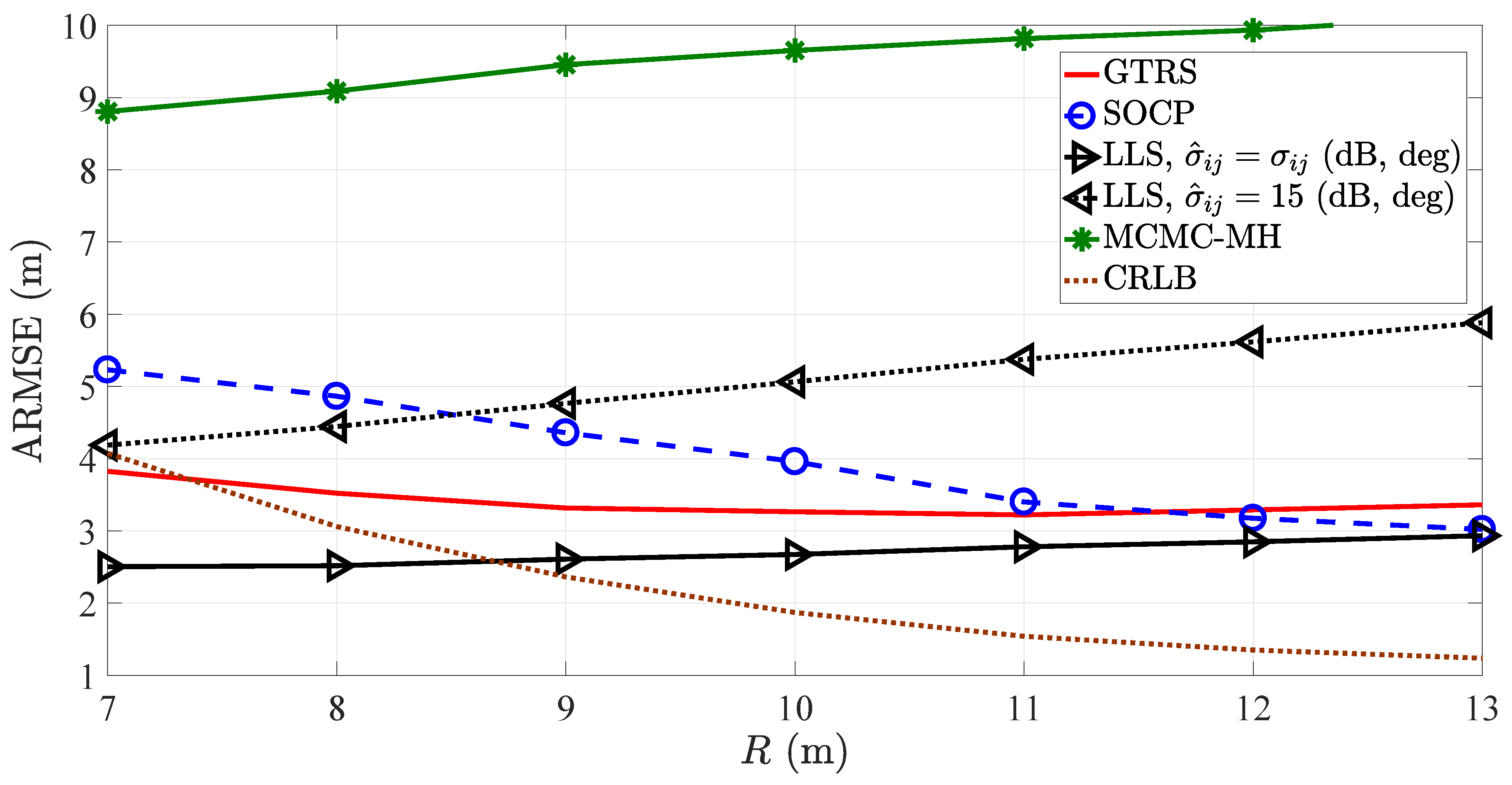
Figure 14 depicts ARMSE (m) versus R (m) comparison for fixed and . One can see from the figure that LLS and GTRS methods are biased for small R (m), since they outperform CRLB in this setting. Furthermore, even though it is intuitive that all methods improve as R (m) is increased, Figure 14 shows that this is not exactly the case. For instance, LLS and MCMC-MH methods worsen with the increase of R, while GTRS improves until a certain point after which it seems to get saturated and its performance worsens slightly after that point. The only method that continuously benefits from the increase of R is SOCP. This can be explained to some extent by the fact that its computational complexity is the highest among the considered methods, which might give it more robustness when processing the additional information caused by increasing R.
5. Summary and Future Prospects
This survey studied the problem of distributed target localization based on amalgamated RSS and AOA measurements. It provided formal mathematical derivation of the problem and presented a set of existing solutions. These state-of-the-art methods were studied from a signal processing perspective and their basic ideas were elaborated without focusing on extensive technical details characteristic to each one of the approaches. An analysis from both computational complexity and localization accuracy point of view was provided in order to give an intuition to the reader about the performance of the existing approaches. Likewise, the most commonly used theoretical lower bound (in the literature) on the localization accuracy was reviewed, as well, with the objective to evaluate the margin for further improvements.
Some of the described approaches in this survey are computationally demanding and some require installing additional hardware (e.g., antenna arrays or directional antennas) on all nodes in the network. The former issue might restrict the applicability of such approaches in real-time or in resource-restrained networks (e.g., battery lives of nodes), at least for the time being. The latter issue raises the question of financial pay off for using such approaches in a wide variety of applications (e.g., in military or fire prevention applications where nodes are deployed in areas where they are likely to be damaged or destroyed). Both issues are equally important and should not be disregarded in the development of future solutions for target localization in general.
The application in fire detection/prevention is very important in countries where the climate favors this hazard, such as Portugal. In the last 20 years, Portugal has been severely affected by large wildfires with dramatic consequences and casualties. Hence, it is urgent that the scientific community provides sound and efficient tools capable of improving decision making during wildfires crisis to minimize its negative consequences. A key component in decision support mechanisms for operational interventions is the information obtained within the network, which might be useless without knowing the location of nodes that acquired the information. Currently, the hardware used in forest surveillance is based on expensive video cameras installed on tall towers, complemented by meteorological sensors. There is no operational decision support system functioning in real-time fed by data provided by the network, mostly because it requires significant resources (human and equipment), which are very limited during wildfires.
In the following years, we expect to see a further boost in the research interest for target localization in general. Our reasoning is founded on the fact that we are living in a period of incessant and rapid development of novel technologies and introduction of new applications. For instance, employing localization technologies to complement and enhance vehicular and pedestrian systems in the fields of intelligent transportation systems, location-based services, robotics, and automated vehicles has already began. Similarly with the line of research presented here, a huge potential for future improvements of localization performance is expected to emerge from a fusion of information coming from already deployed (or novel) infrastructures (e.g., signals of opportunity), as well as the use of crowd sensing, owing to the widespread use of smartphones today.
The forthcoming technologies (5G and IoT) will continue attracting the research interest towards distributed target localization without a doubt. It is expected that the IoT will continue nourishing the growth of networks in their size and their dynamics. Due to the augmented network size and node mobility, implementation of localization algorithms in a distributed manner will become a requirement for many practical settings, like smart buildings and smart cities. As a direct consequence, this will stimulate researchers to develop novel signal processing approaches for efficient (accurate and fast) distributed localization solutions. Furthermore, we expect that all these activities will require some level of security; hence, we expect that secure localization (localization in the presence of one or more malicious/corrupted nodes) will attract many research interest in the upcoming years. This is because today’s localization systems are susceptible to location spoofing, where devices can deceive other devices with regards to their own locations or can manipulate the measured locations of other devices [73].
Finally, we saw that node cooperation does not bring benefit by default for any of the considered estimators (e.g., when M and/or R (m) is increased). From the localization accuracy perspective, this result is very important since it indicates that there is still room for improvements, as it was also confirmed by comparing the methods against the theoretical bound. Essentially, this might imply that unlimited node cooperation is not the solution for the localization problem at hand, or simply that one needs to come up with a better way to exploit the additional information due to node cooperation in order to benefit from it.
Author Contributions
All authors were involved in the mathematical developments and writing of the paper. The computer simulations were carried out by S.T. All authors have read and agree to the published version of the manuscript. All authors have read and agreed to the published version of the manuscript.
Funding
This work was partially supported by Fundação para a Ciência e a Tecnologia under Projects UID/EEA/00066/2019, foRESTER PCIF/SSI/0102/2017, and IF/00325/2015.
Conflicts of Interest
The authors declare no conflict of interest.
Appendix A. CRLB Derivation for RSS-AOA Localization
In estimation theory and statistics, the CRLB gives a lower bound on the variance of unbiased estimators of a deterministic (fixed, though unknown) parameter [56] (Chapter 3). Loosely speaking, the bound states that the variance of any unbiased estimator is at least as high as the inverse of the FIM. Thus, the CRLB is a reference point against which the performance of unbiased estimators can be analyzed.
According to the definition [56] (Chapter 3), the variance of any unbiased localization estimator is lower bounded by , where is the FIM. The elements of the FIM are defined as , where , and is the joint conditional probability density function of the observation vector , given .
Therefore, it follows that the FIM can be computed as:
where and are the anchor and target neighborhoods of the i-th target,
, with representing the i-th column of the identity matrix , and , .
Therefore, the CRLB for the estimate of the target locations is computed as:
References
- Coluccia, A. Reduced-bias ML-based Estimators with Low Complexity for Self-calibrating RSS Ranging. IEEE Trans. Wirel. Commun. 2014, 12, 1220–1230. [Google Scholar] [CrossRef]
- Beko, M. Energy-based Localization in Wireless Sensor Networks Using Second-order Cone Programming Relaxation. Wirel. Pers. Commun. 2014, 77, 1847–1857. [Google Scholar] [CrossRef]
- Coluccia, A.; Ricciato, F. RSS-based Localization via Bayesian Ranging and Iterative Least Squares Positioning. IEEE Commun. Lett. 2014, 18, 836–876. [Google Scholar] [CrossRef]
- Tomic, S.; Beko, M.; Dinis, R. 3-D Target Localization in Wireless Sensor Network Using RSS and AoA Measurement. IEEE Trans. Vehic. Technol. 2017, 66, 3197–3210. [Google Scholar] [CrossRef]
- Tomic, S.; Beko, M.; Dinis, R.; Tuba, M.; Bacanin, N. Bayesian Methodology for Target Tracking Using RSS and AoA Measurements. Phys. Commun. 2017, 25, 158–166. [Google Scholar] [CrossRef] [Green Version]
- Correia, S.; Beko, M.; Cruz, L.; Tomic, S. Elephant Herding Optimization for Energy-Based Localization. Sensors 2018, 18, 2849. [Google Scholar]
- Tomic, S.; Beko, M.; Tuba, M.; Correia, V.M.F. Target Localization in NLOS Environments Using RSS and TOA Measurements. IEEE Wirel. Commun. Lett. 2018, 7, 1062–1065. [Google Scholar] [CrossRef] [Green Version]
- Pedro, D.; Tomic, S.; Bernardo, L.; Beko, M.; Oliveira, R.; Dinis, R.; Pinto, P.; Amaral, P. Algorithms for Estimating the Location of Remote Nodes Using Smartphones. IEEE Access 2019, 17, 33713–33727. [Google Scholar] [CrossRef]
- Tomic, S.; Beko, M.; Dinis, R.; Gomes, J.P. Target Tracking with Sensor Navigation Using Coupled RSS and AOA Measurements. Sensors 2017, 17, 2690. [Google Scholar] [CrossRef] [Green Version]
- Bandiera, F.; Coluccia, A.; Ricci, G. A Cognitive Algorithm for Received Signal Strength Based Localization. IEEE Trans. Signal Process. 2015, 63, 1726–1736. [Google Scholar] [CrossRef]
- Tomic, S.; Beko, M. Exact Robust Solution to TW-ToA-based Target Localization Problem with Clock Imperfections. IEEE Signal Process. Lett. 2018, 25, 531–535. [Google Scholar] [CrossRef] [Green Version]
- Coluccia, A.; Fascista, A. On the Hybrid TOA/RSS Range Estimation in Wireless Sensor Networks. IEEE Trans. Wirel. Commun. 2018, 17, 361–371. [Google Scholar] [CrossRef]
- Carlino, L.; Bandiera, F.; Coluccia, A.; Ricci, G. Improving Localization by Testing Mobility. IEEE Trans. Signal Process. 2019, 67, 3412–3423. [Google Scholar] [CrossRef]
- Tomic, S.; Beko, M.; Dinis, R.; Tuba, M.; Bacanin, N. RSS-AOA-based Target Localization and Tracking in Wireless Sensor Networks, 1st ed.; River Publishers: Delft, The Netherlands, 2017. [Google Scholar]
- Tomic, S.; Beko, M.; Tuba, M. A Linear Estimator for Network Localization Using Integrated RSS and AOA Measurements. IEEE Signal Process. Lett. 2019, 26, 405–409. [Google Scholar] [CrossRef] [Green Version]
- Coluccia, A.; Fascista, A. Hybrid TOA/RSS Range-Based Localization with Self-Calibration in Asynchronous Wireless Networks. J. Sens. Actuator Netw. 2019, 8, 31. [Google Scholar] [CrossRef] [Green Version]
- Tomic, S.; Beko, M. A Bisection-based Approach for Exact Target Localization in NLOS Environments. Signal Process. 2018, 143, 328–335. [Google Scholar] [CrossRef] [Green Version]
- Tomic, S.; Beko, M.; Dinis, R.; Montezuma, P. A Robust Bisection-based Estimator for TOA-based Target Localization in NLOS Environments. IEEE Commun. Lett. 2017, 21, 2488–2491. [Google Scholar] [CrossRef] [Green Version]
- Safavi, S.; Khan, U.A.; Kar, S.; Moura, J.M.F. Estimating Directional Data From Network Topology for Improving Tracking Performance. Proc. IEEE 2018, 106, 1204–1223. [Google Scholar] [CrossRef]
- Tomic, S.; Beko, M.; Dinis, R.; Bernardo, L. On Target Localization Using Combined RSS and AoA Measurements. Sensors 2018, 18, 1266. [Google Scholar] [CrossRef] [Green Version]
- Tomic, S.; Beko, M. A Robust NLOS Bias Mitigation Technique for RSS-TOA-based Target Localization. IEEE Signal Process. Lett. 2019, 26, 64–68. [Google Scholar] [CrossRef]
- Pahlavan, K.; Krishnamurthy, P.; Geng, Y. Localization Challenges for the Emergence of the Smart World. IEEE Access 2015, 3, 3058–3067. [Google Scholar] [CrossRef]
- Yang, Z.; Wu, C.; Zhou, Z.; Zhang, X.; Wang, X.; Liu, Y. A Review of Advanced Localization Techniques for Crowdsensing Wireless Sensor Networks. ACM Comput. Surv. 2015, 47, 1–34. [Google Scholar] [CrossRef]
- Han, G.; Jiang, J.; Zhang, C.; Duong, T.Q.; Guizani, M.; Karagiannidis, G.K. A Survey on Mobile Anchor Node Assisted Localization in Wireless Sensor Networks. IEEE Commun. Surv. Tutorials 2016, 18, 2220–2243. [Google Scholar] [CrossRef]
- Coluccia, A.; Fascista, A. A Review of Advanced Localization Techniques for Crowdsensing Wireless Sensor Networks. Sensors 2019, 19, 988. [Google Scholar] [CrossRef] [PubMed] [Green Version]
- Camarinha-Matos, L.M.; Afsarmanesh, H. Roots of Collaboration: Nature-Inspired Solutions for Collaborative Networks. IEEE Access 2018, 6, 30829–30843. [Google Scholar] [CrossRef]
- Witrisal, K.; Meissner, P.; Leitinger, E.; Shen, Y.; Gustafson, C.; Tufvesson, F.; Haneda, K.; Dardari, D.; Molisch, A.F.; Conti, A.; et al. High-Accuracy Localization for Assisted Living: 5G systems will turn multipath channels from foe to friend. IEEE Signal Process. Mag. 2016, 33, 59–70. [Google Scholar] [CrossRef]
- Abu-Shaban, Z.; Zhou, X.; Abhayapala, T.; Seco-Granados, G.; Wymeersch, H. Error Bounds for Uplink and Downlink 3D Localization in 5G Millimeter Wave Systems. IEEE Trans. Wirel. Commun. 2018, 17, 4939–4954. [Google Scholar]
- Fascista, A.; Coluccia, A.; Wymeersch, H.; Seco-Granados, G. Millimeter-Wave Downlink Positioning With a Single-Antenna Receiver. IEEE Trans. Wirel. Commun. 2019, 18, 4479–4490. [Google Scholar] [CrossRef] [Green Version]
- Singh, Y.; Saha, S.; Chugh, U.; Gupt, C. Distributed Event Detection in Wireless Sensor Networks for Forest Fires. In Proceedings of the 2013 UKSim 15th International Conference on Computer Modelling and Simulation, Cambridge, UK, 10–12 April 2013; pp. 634–639. [Google Scholar]
- Madeira, R.; Paulino, N. Analysis and Implementation of a Power Management Unit with a Multiratio Switched Capacitor DC–DC Converter for a Supercapacitor Power Supply. Int. J. Circuit Theory Appl. 2016, 44, 2018–2034. [Google Scholar] [CrossRef]
- Nowacki, B.; Paulino, N.; Goes, J. A Third-Order MASH ΣΔ Modulator Using Passive Integrators. IEEE Trans. Circuits Syst. Regul. Pap. 2017, 64, 2871–2883. [Google Scholar] [CrossRef]
- Tahat, A.; Kaddoum, G.; Yousefi, S.; Valaee, S.; Gagnon, F. A Look at the Recent Wireless Positioning Techniques With a Focus on Algorithms for Moving Receivers. IEEE Access 2016, 4, 6652–6680. [Google Scholar] [CrossRef]
- Tomic, S.; Beko, M.; Dinis, R.; Montezuma, P. Distributed Algorithm for Target Localization in Wireless Sensor Networks Using RSS and AoA Measurements. Pervasive Mob. Comput. 2017, 37, 63–77. [Google Scholar] [CrossRef] [Green Version]
- Zamiri, M.; Camarinha-Matos, L.M. Mass Collaboration and Learning: Opportunities, Challenges, and Influential Factors. Appl. Sci. 2019, 9, 2620. [Google Scholar] [CrossRef] [Green Version]
- Vafaei, N.; Ribeiro, R.A.; Camarinha-Matos, L.M.; Valera, L.R. Normalization Techniques for Collaborative Networks. Kybernetes 2019, X, X–Z. [Google Scholar] [CrossRef]
- Vaghefi, R.M.; Buehrer, R.M. Cooperative Localization in NLOS Environments Using Semidefinite Programming. IEEE Commun. Lett. 2015, 19, 1382–1385. [Google Scholar] [CrossRef]
- Khan, M.W.; Salman, N.; Kemp, A.H. Optimised Hybrid Localisation with Cooperation in Wireless Sensor Networks. IET Signal Process. 2017, 11, 341–348. [Google Scholar] [CrossRef]
- Tomic, S.; Beko, M. Target Localization via Integrated and Segregated Ranging Based on RSS and TOA Measurements. Sensors 2019, 19, 230. [Google Scholar] [CrossRef] [Green Version]
- Tomic, S.; Beko, M.; Dinis, R. Distributed RSS-Based Localization in Wireless Sensor Networks Based on Second-Order Cone Programming. Sensors 2014, 14, 18410–18432. [Google Scholar] [CrossRef] [Green Version]
- Patwari, N. Location Estimation in Sensor Networks. Ph.D. Thesis, University of Michigan, Ann Arbor, MI, USA, 2005. [Google Scholar]
- Rappaport, T.S. Wireless Communications: Principles and Practice, 1st ed.; Prentice Hall: Upper Saddle River, NJ, USA, 1996. [Google Scholar]
- Sichitiu, M.L.; Ramadurai, V. Localization of Wireless Sensor Networks with a Mobile Beacon. In Proceedings of the 2004 IEEE International Conference on Mobile Ad-hoc and Sensor Systems, Fort Lauderdale, FL, USA, 25–27 October 2004; pp. 174–183. [Google Scholar]
- Tomic, S.; Beko, M.; Dinis, R. RSS-based Localization in Wireless Sensor Networks Using Convex Relaxation: Noncooperative and Cooperative Schemes. IEEE Trans. Veh. Technol. 2015, 64, 2037–2050. [Google Scholar] [CrossRef] [Green Version]
- Kulas, L. RSS-Based DoA Estimation Using ESPAR Antennas and Interpolated Radiation Patterns. IEEE Antennas Wirel. Propag. Lett. 2018, 17, 25–28. [Google Scholar] [CrossRef]
- Niculescu, D.; Nath, B. VOR Base Stations for Indoor 802.11 Positioning. In Proceedings of the 10th annual international conference on Mobile computing and networking, Philadelphia, PA, USA, 26 September–1 October 2004; pp. 58–69. [Google Scholar]
- Ferreira, M.B.; Gomes, J.; Costeira, J.P. A Unified Approach for Hybrid Source Localization Based on Ranges and Video. In Proceedings of the 2015 IEEE International Conference on Acoustics, Speech and Signal Processing (ICASSP), Brisbane, QLD, Australia, 19–24 April 2015; pp. 2879–2883. [Google Scholar]
- Tomic, S.; Beko, M.; Dinis, R.; Montezuma, P. Estimating Directional Data From Network Topology for Improving Tracking Performance. J. Sens. Actuator Netw. 2019, 8, 30. [Google Scholar] [CrossRef] [Green Version]
- Schmidt, R. Multiple emitter location and signal parameter estimation. IEEE Trans. Antennas Propag. 1986, 34, 276–280. [Google Scholar] [CrossRef] [Green Version]
- Roy, R.; Kailath, T. ESPRIT-estimation of signal parameters via rotational invariance techniques. IEEE Trans. Acoust. Speech Signal Process. 1989, 37, 984–995. [Google Scholar] [CrossRef] [Green Version]
- Yu, K. 3-D Localization Error Analysis in Wireless Networks. IEEE Trans. Wirel. Commun. 2007, 6, 3473–3481. [Google Scholar]
- Fascista, A.; Ciccarese, G.; Coluccia, A.; Ricci, G. Angle of Arrival-Based Cooperative Positioning for Smart Vehicles. IEEE Trans. Intell. Transp. Syst. 2018, 19, 2880–2892. [Google Scholar] [CrossRef]
- Tomic, S.; Beko, M.; Dinis, R.; Montezuma, P. A Closed-form Solution for RSS/AoA Target Localization by Spherical Coordinates Conversion. IEEE Wirel. Commun. Lett. 2016, 5, 680–683. [Google Scholar] [CrossRef] [Green Version]
- Mardia, K.V. Statistics of Directional Data, 1st ed.; Academic Press, Inc.: London, UK, 1972. [Google Scholar]
- Forbes, C.; Evans, M.E.; Hastings, N.; Peacock, B. Statistical Distributions, 4th ed.; John Wiley & Sons, Inc.: Hoboken, NJ, USA, 2011. [Google Scholar]
- Kay, S.M. Fundamentals of Statistical Signal Processing: Estimation Theory, 1st ed.; Prentice Hall: Upper Saddle River, NJ, USA, 1993. [Google Scholar]
- Li, X.R.; Zhao, Z. Measures of Performance for Evaluation of Estimators and Filters. In Signal and Data Processing of Small Targets 2001; Drummond, O., Ed.; SPIE: San Diego, CA, USA, 2001; Volume 4473, pp. 1–12. [Google Scholar]
- Dardari, D.; Closas, P.; Djuric, P.M. Indoor Tracking: Theory, Methods, and Technologies. IEEE Trans. Veh. Technol. 2016, 64, 1263–1278. [Google Scholar] [CrossRef] [Green Version]
- Patwari, N.; Ash, J.N.; Kyperountas, S.; Hero, A.O., III; Moses, R.L.; Correal, N.S. Locating the Nodes: Cooperative Localization in Wireless Sensor Networks. IEEE Signal Process. Mag. 2005, 22, 54–69. [Google Scholar] [CrossRef]
- Hashemi, H. The Indoor Radio Propagation Channel. Proc. IEEE 1993, 81, 943–968. [Google Scholar] [CrossRef]
- Tomic, S.; Beko, M.; Dinis, R. Distributed RSS-AoA Based Localization with Unknown Transmit Powers. IEEE Wirel. Commun. Lett. 2016, 5, 392–395. [Google Scholar] [CrossRef]
- Boyd, S.; Vandenberghe, L. Convex Optimization, 1st ed.; Cambridge University Press: Cambridge, UK, 2004. [Google Scholar]
- Grant, M.; Boyd, S. CVX: MATLAB Software for Disciplined Convex Programming; CVX Research, Inc.: Austin, TX, USA, 2003. [Google Scholar]
- Coluccia, A.; Ricciato, F.; Ricci, G. Positioning Based on Signals of Opportunity. IEEE Commun. Lett. 2014, 18, 356–359. [Google Scholar] [CrossRef]
- Naseri, H.; Koivunen, V. A Bayesian Algorithm for Distributed Network Localization Using Distance and Direction Data. IEEE Trans. Signal Inf. Process. Over Netw. 2019, 5, 290–304. [Google Scholar] [CrossRef]
- Robert, C.; Casella, G. Introducing Monte Carlo Methods with R, 1st ed.; Springer: Berlin, Germany, 2009. [Google Scholar]
- Koller, D.; Friedman, N. Probabilistic Graphical Models: Principles and Techniques, 1st ed.; MIT Press: Cambridge, MA, USA, 2009. [Google Scholar]
- Tomic, S.; Beko, M. A Geometric Approach for Distributed Multi-hop Target Localization in Cooperative Networks. Accept. Publ. IEEE Trans. Veh. Technol. 2019, X, X–Y. [Google Scholar] [CrossRef]
- Moré, J.J. Generalization of the Trust Region Problem. Optim. Meth. Soft. 1993, 2, 189–209. [Google Scholar] [CrossRef]
- Beck, A.; Stoica, P.; Li, J. Exact and Approximate Solutions of Source Localization Problems. IEEE Trans. Signal Process. 2008, 56, 1770–1778. [Google Scholar] [CrossRef]
- Ergen, S.C.; Varaiya, P. TDMA Scheduling Algorithms for Wireless Sensor Networks. Wirel. Netw. 2010, 16, 985–997. [Google Scholar] [CrossRef] [Green Version]
- Mota, J.F.C.; Xavier, J.M.F.; Aguiar, P.M.Q.; Püschel, M. D-ADMM: A Communication-Efficient Distributed Algorithm for Separable Optimization. Wirel. Netw. 2013, 61, 2718–2723. [Google Scholar] [CrossRef] [Green Version]
- Singh, M.; Leu, P.; Abdou, A.R.; Capkun, S. UWB-ED: Distance Enlargement Attack Detection in Ultra-Wideband. In Proceedings of the 28th USENIX Security Symposium (USENIX Security 19), Santa Clara, CA, USA, 14–16 August 2019; pp. 73–88. [Google Scholar]
Figure 1.
Application of a wireless sensor network in forest firefighting.

Figure 2.
Illustration of different network types based on the type of communication.

Figure 3.
Illustration of different network types based on the type of processing. CN = central node.
Figure 3.
Illustration of different network types based on the type of processing. CN = central node.

Figure 4.
Illustration of the considered model in 2-dimensional space.

Figure 5.
Illustration of angle of arrival (AOA) estimation process based on the received signal strength (RSS) ratio, , between two directional antennas.
Figure 5.
Illustration of angle of arrival (AOA) estimation process based on the received signal strength (RSS) ratio, , between two directional antennas.

Figure 6.
Illustration of the second-order (Lorentz) cone in : .

Figure 7.
Illustration of the process of convex relaxation.

Figure 8.
Illustration of the least-squares fitting method.

Figure 9.
Illustration of the Markov chain Monte Carlo with Metropolis-Hastings (MCMC-MH) procedure.
Figure 9.
Illustration of the Markov chain Monte Carlo with Metropolis-Hastings (MCMC-MH) procedure.

Figure 10.
Illustration of the geometric approach in [68] for a 2-hop case.
Figure 10.
Illustration of the geometric approach in [68] for a 2-hop case.

Figure 11.
Illustration of the generalized trust region sub-problem (GTRS) solved by a bisection procedure.
Figure 11.
Illustration of the generalized trust region sub-problem (GTRS) solved by a bisection procedure.

Figure 12.
Average root mean square error (ARMSE) (m) versus N: , m, . CRLB = Cramér-Rao lower bound (CRLB).
Figure 12.
Average root mean square error (ARMSE) (m) versus N: , m, . CRLB = Cramér-Rao lower bound (CRLB).

Figure 13.
ARMSE (m) versus M: , m, .

Figure 14.
ARMSE (m) versus R (m): , , .


Table 1.
Summary of the main characteristics of the considered algorithms. SOCP = second-order cone programming; LLS = linear least squares; MCMC-MH = Markov chain Monte Carlo with Metropolis-Hastings.
Table 1.
Summary of the main characteristics of the considered algorithms. SOCP = second-order cone programming; LLS = linear least squares; MCMC-MH = Markov chain Monte Carlo with Metropolis-Hastings.
| Algorithm | RSS | AOA | Noise STD | |
|---|---|---|---|---|
| SOCP | All nodes | Anchors | Not known/Known | Unknown |
| LLS | All nodes | All nodes | Known | Known |
| MCMC-MH | All nodes | All nodes | Known | Known |
| GTRS | All nodes | Anchors | Known | Unknown |
Table 2.
Analysis of computational complexity and average execution time.
| Algorithm | Complexity | Time (sec) |
|---|---|---|
| SOCP | 0.66 | |
| LLS | 0.004 | |
| MCMC-MH | 1.2 | |
| GTRS | 0.005 |
© 2019 by the authors. Licensee MDPI, Basel, Switzerland. This article is an open access article distributed under the terms and conditions of the Creative Commons Attribution (CC BY) license (http://creativecommons.org/licenses/by/4.0/).
Share and Cite
MDPI and ACS Style
Tomic, S.; Beko, M.; Camarinha-Matos, L.M.; Oliveira, L.B. Distributed Localization with Complemented RSS and AOA Measurements: Theory and Methods. Appl. Sci. 2020, 10, 272. https://0-doi-org.brum.beds.ac.uk/10.3390/app10010272
AMA Style
Tomic S, Beko M, Camarinha-Matos LM, Oliveira LB. Distributed Localization with Complemented RSS and AOA Measurements: Theory and Methods. Applied Sciences. 2020; 10(1):272. https://0-doi-org.brum.beds.ac.uk/10.3390/app10010272
Chicago/Turabian StyleTomic, Slavisa, Marko Beko, Luís M. Camarinha-Matos, and Luís Bica Oliveira. 2020. "Distributed Localization with Complemented RSS and AOA Measurements: Theory and Methods" Applied Sciences 10, no. 1: 272. https://0-doi-org.brum.beds.ac.uk/10.3390/app10010272
Note that from the first issue of 2016, this journal uses article numbers instead of page numbers. See further details here.