Coupling Control Strategy and Experiments for Motion Mode Switching of a Novel Electric Chassis

Abstract

A flexible chassis (FC) is a type of electric vehicle driven by in-wheel motors that can be used in narrow conditions in agricultural facilities. The FC is composed primarily of four off-center steering mechanisms (OSMs) that can be controlled independently. Various FC operation modes can be achieved including cross motion (CM), in-place rotation (IR), diagonal motion (DM), and steering motion (SM). However, it is difficult to achieve satisfactory motion mode switching (MMS) results under traditional distribution control methodologies due to a lack of linkage relationships between the four OSMs. The goal of this study was to provide a coupling control method that can cope with this problem. First, dynamic MMS models were derived. Then, an MMS coupling error (CE) model was derived based on coupling control and Lyapunov stability theory. Second, a fuzzy proportional integral derivative (PID) controller with self-tuning parameters was designed to reduce the CE during MMS. A fuzzy PI controller was also employed to improve response times and decrease OSM tracking motion steady-state error. Finally, MATLAB/Simulink simulations were performed and experimentally validated on hard pavement. The results showed that the proposed methodology could effectively reduce CE and guarantee MMS control stability while substantially shortening response times. The proposed methodology is effective and feasible for FC MMS.

1. Introduction

Narrow, confined agricultural facilities such as greenhouses, orchards, and warehouses have difficult vehicle requirements. Vehicles used in these facilities must be flexible and protect the environment [1,2]. Currently, most transportation equipment used in these facilities is within the category of small conventional vehicles such as tractors, tricycles, mobile platforms, etc. Most of these vehicles are equipped with traditional powertrain systems. Inflexibility and exhaust emissions are two main problems with this equipment [3,4]. It is critical to develop flexible, environmentally friendly, energy-sustainable vehicles for agricultural facility environments [5,6,7].

Electric vehicles (EVs) with four in-wheel motors have attracted tremendous attention in recent years because of their actuation flexibility [8,9]. By taking advantage of distributed driving modes and steer-by-wire systems, each wheel can operate to its maximum capacity and the vehicle structure can be simplified radically. In addition, the electrification of agricultural machinery is essential to promoting energy independence and efficiency, and will eventually aid in cost reduction [10]. Therefore, this vehicle technology has the potential to solve the previously mentioned problems in agriculture. However, several challenges must be overcome for this type of vehicle to be made available. These challenges involve over-actuation, high control system complexity, and severe coordinated control requirements [11,12,13]. Thus, this study focuses on the motion control problem of a flexible electric vehicle, referred to as a flexible chassis (FC). The FC is a chassis with four independently driven in-wheel motors that can flexibly perform multiple types of motion, making it suitable for confined facility environments.

Numerous valuable studies of EV control methodology were recently conducted in agricultural facility machinery areas. These studies mainly involved objects such as electric chassis, mobile robots, and electric platforms. Gat et al. developed a steering control algorithm based on an overhead guide to improve the stability of an autonomous greenhouse harvesting and spraying vehicle [14]. Based on sliding mode control, Tu et al. proposed a robust controller for a four-wheel drive and steering agricultural vehicle. The researchers demonstrated good controller capabilities and robustness in controlling a system with a high degree of freedom [15]. Kannan et al. designed a fuzzy logic controller to adjust drive wheel speed and achieved teleoperated steering for agricultural vehicles [16]. Ma and Qi designed a general-purpose electric chassis for agricultural tasks such as mapping, detection, guidance, and action based on human-centered design frameworks and processes [17].

Various researchers have focused on mobile robots due to agricultural facility equipment intelligence requirements. Qiu et al. proposed a novel extended Ackerman steering principle for an agricultural mobile robot. Compared with the conventional Ackerman steering principle, the proposed strategy can reduce the energy consumption of the entire machine [18]. Wang et al. introduced a proportional integral derivative (PID) algorithm into a laser navigation control system. Their study achieved low-speed steering control of a greenhouse tomato-harvesting robot based on the Ackerman steering principle [19]. Grimstad and From proposed a two-stage guidance control scheme for a low-cost planting robot. This system could regulate the direction of the robot and minimize the lateral error associated with navigation [20].

Classical control methods such as PID control methodology, the frequency response, and root locus methods have been commonly used to improve overall EV performance. However, these methods require complex, precise modeling [21,22,23,24,25] and are incapable of tackling the nonlinear problem of EVs [26]. Intelligent control methods such as artificial neural networks, genetic algorithms, and fuzzy logic can be implemented in engineering practice more easily and effectively than classical control methods. For example, Nguyen et al. proposed a class of constrained Takagi–Sugeno fuzzy system with a simple control structure and a low level of numerical complexity. That study provided better results than some recent works developed in a non-quadratic Lyapunov framework [27]. In addition, the fuzzy method they developed can also be used to handle a large variation range of vehicle speed [28]. In general, these algorithms have recently been targets of rapid development [29]. They can cope with the nonlinear problems that affect almost all EVs without exact mathematical models [30].

However, most EV studies utilize separate drive and steering systems. Vehicle structures have become complex, thus complicated manufacturing engineering is required. These proposed control strategies have focused mainly on the stability and efficiency of the steering system, or the drivability and safety of the driving system. Few studies have considered a combined steering–driving system for EVs. In the case of the FC, a kind of off-center steering shaft mechanism (OSM) is utilized. The drive and steering systems are combined because the forces involved in both driving and steering come from the in-wheel motor [31]. For this reason, the FC structure is quite simple. It can achieve multiple motion modes, including cross motion (CM), in-place rotation (IR), diagonal motion (DM), and steering motion (SM), and can be used flexibly in narrow or closed environments. The FC is expected to be used for low-speed transportation work in greenhouses, warehouses, or orchards. Flexible motion mode switching (MMS) based on OSM provides the chassis with the ability to adapt to difficult environments. Namely, the posture of the chassis can be adjusted according to different work environments. The high ground clearance and suspension also allow it to adapt to uneven roads [32]. However, due to the lack of a rigid constraint mechanism, it is difficult to coordinate the motion of each FC OSM during MMS in situ.

The objective of this paper is to provide a coordinated control strategy to reduce MMS angular velocity coupling errors (CEs) and guarantee smooth, steady MMS. To achieve this, a CE model is derived based on coupling control and Lyapunov stability theory. A fuzzy PID controller is then designed for CE control. To shorten the response time and reduce steady-state errors of OSM steering tracking motion, a fuzzy PI control method is employed for steering tracking control. The feasibility of the proposed control strategy is confirmed via MATLAB/Simulink simulations and then experimentally validated on hard pavement. This paper provides two main contributions to the engineering community: (i) a control algorithm that integrates coupling control, Lyapunov stability theory, fuzzy PID control, and fuzzy PI control is proposed for FC MMS in order to cope with the lack of a linkage relationship among the four OSMs, and (ii) the CE performance and MMS stability are improved under the proposed control methodology.

The rest of the paper is organized as follows. In Section 2, the overall structure of the FC and system modeling are described. In Section 3, a coupling control strategy for MMS of the FC is designed. In Section 4, we discuss the MATLAB/Simulink simulation. Section 5 is dedicated to experimental validation. Finally, our conclusions and proposals for future work are provided in Section 6.

2. Problem Formulation and System Modeling

2.1. Overall Structure

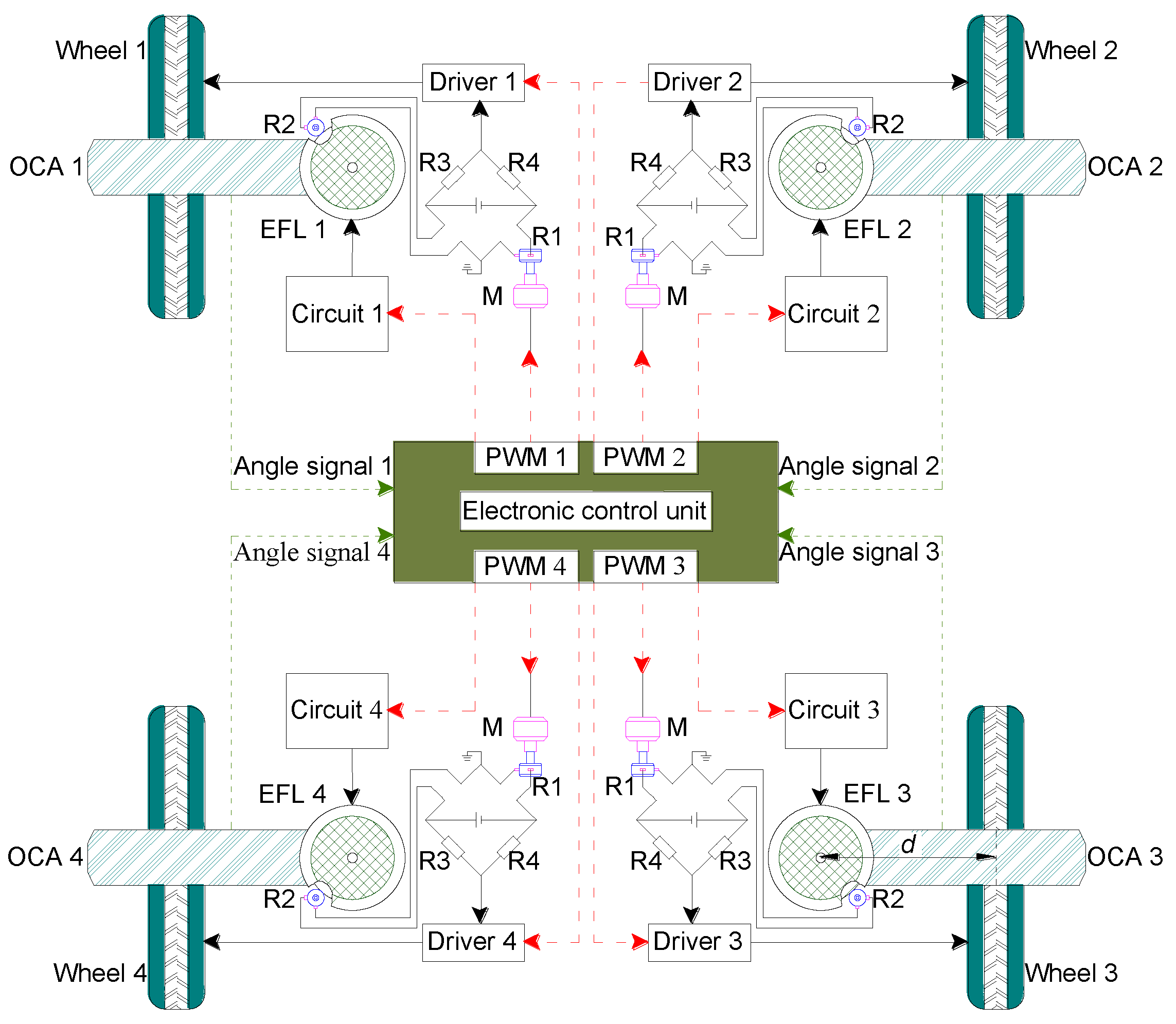
The overall structure of the FC drawn by Computer Aided Design (AutoCAD2007, Auto desk Company, San Rafael, CA, USA) is shown in Figure 1. The main components include four OSMs, an electronic control unit, and the control lines.

Each OSM consists of an electromagnetic friction lock (FBD-050, Taiwan Kaide, Taiwan), an off-center steering shaft, an off-center arm, a suspension and an in-wheel motor (WX-WS4846, Fujitec, Tianjin, China. A bridge circuit made of four arms identified as R1, R2, R3, and R4 achieves steering tracking for the OSM. When the electromagnetic friction lock is in a release state, the vehicle is flexibly steered by rotating the OSM around the steering shaft. By controlling the electromagnetic friction locks and the in-wheel motors, the FC can achieve the various types of motion modes mentioned earlier. Switching processes of all motion modes are performed in situ during MMS. In contrast, when the electromagnetic friction lock is in a locked state, the off-center arm is fixed on the FC frame and the FC can only move with fixed posture. This paper focuses on the MMS coupling control methodology.

2.2. Motion Models for Various Motion Modes

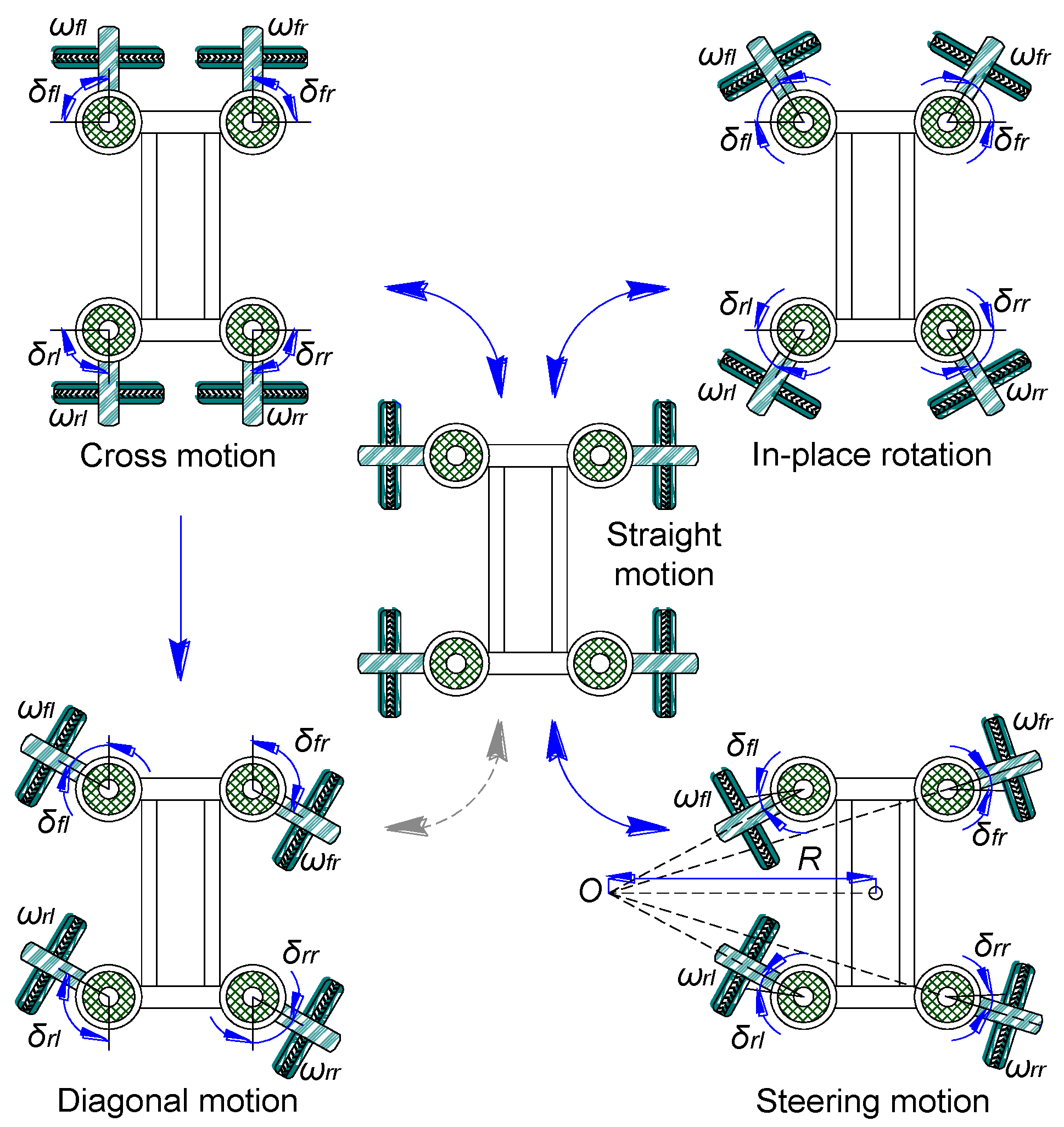
A schematic diagram of the FC motion mode models is presented in Figure 2. Different motion modes require different off-center arm steering angles. During MMS, the steering angles of the four off-center arms and the angular velocities of the four in-wheel motors must maintain fixed relationships. Each off-center arm has a specific target angle. During CM, the relationships are given by:

$$\{\begin{array}{l}\left|{\delta }_{flo}\right|=\left|{\delta }_{fro}\right|=\left|{\delta }_{rlo}\right|=\left|{\delta }_{rro}\right|=\frac{\pi }{2},{\delta }_{fl}=-{\delta }_{fr}={\delta }_{rl}=-{\delta }_{rr}\\ {\omega }_{fl}={\omega }_{fr}={\omega }_{rl}={\omega }_{rr}\end{array},$$

(1)

where δ_i is the steering angle of each off-center arm (I = fl, fr, rl, rr, which represent the left front, right front, left rear, and right rear wheel of the flexible chassis, respectively), ω_i is the angular velocity of each off-center steering mechanism, and δ_io denote the target angle of each off-center arm.

For in-place rotation, the target angles and angular velocities have the following relationships:

$$\{\begin{array}{l}\left|{\delta }_{flo}\right|=\left|{\delta }_{fro}\right|=\left|{\delta }_{rlo}\right|=\left|{\delta }_{rro}\right|=\arctan (\frac{L}{B}),{\delta }_{fl}=-{\delta }_{fr}={\delta }_{rl}=-{\delta }_{rr}\\ {\omega }_{fl}={\omega }_{fr}={\omega }_{rl}={\omega }_{rr}\end{array},$$

(2)

where L is the distance between the front and rear off-center shafts and B is the distance between the left and right off-center shafts.

During the whole MMS process, the FC frame needs to keep its original posture. For diagonal motion, if CM is directly switched to DM, the moments at centroid from all wheels will be in the same direction, and the FC frame cannot keep its posture. To avoid this problem, DM is switched from IR in this study. This method can maintain symmetrical force on the FC. The target angle and angular velocity relationships are expressed by:

$$\{\begin{array}{l}\left|3{\delta }_{flo}\right|=\left|{\delta }_{fro}\right|=\left|3{\delta }_{rlo}\right|=\left|{\delta }_{rro}\right|=\frac{3\pi }{4},{\delta }_{fl}=\pi -{\delta }_{fr}={\delta }_{rl}=\pi -{\delta }_{rr}\\ 3{\omega }_{fl}={\omega }_{fr}=3{\omega }_{rl}={\omega }_{rr}\end{array}.$$

(3)

Similarly, the relationships that govern steering motion are:

$$\{\begin{array}{c}\left|{\delta }_{flo}\right|=\left|\pi -{\delta }_{rlo}\right|=\pi -\arctan (\frac{2L}{2R+B}),\left|{\delta }_{fro}\right|=\left|\pi -{\delta }_{rro}\right|=\arctan (\frac{2L}{2R-B})\hfill \\ {\delta }_{fl}=\pi -{\delta }_{rl},{\delta }_{fr}=\pi -{\delta }_{rr}\hfill \\ {\omega }_{fl}:{\omega }_{fr}:{\omega }_{rl}:{\omega }_{rr}=\left|\sqrt{{(R+0.5B)}^2+L^2}+d\right|:\left|\sqrt{{(R-0.5B)}^2+L^2}-d\right|\hfill \\ :\left|\sqrt{{(R-0.5B)}^2+L^2}-d\right|:\left|\sqrt{{(R+0.5B)}^2+L^2}+d\right|\end{array},$$

(4)

where d is the off-center distance and R is the turning radius of the FC during steering motion.

2.3. Model of Electric Wheel

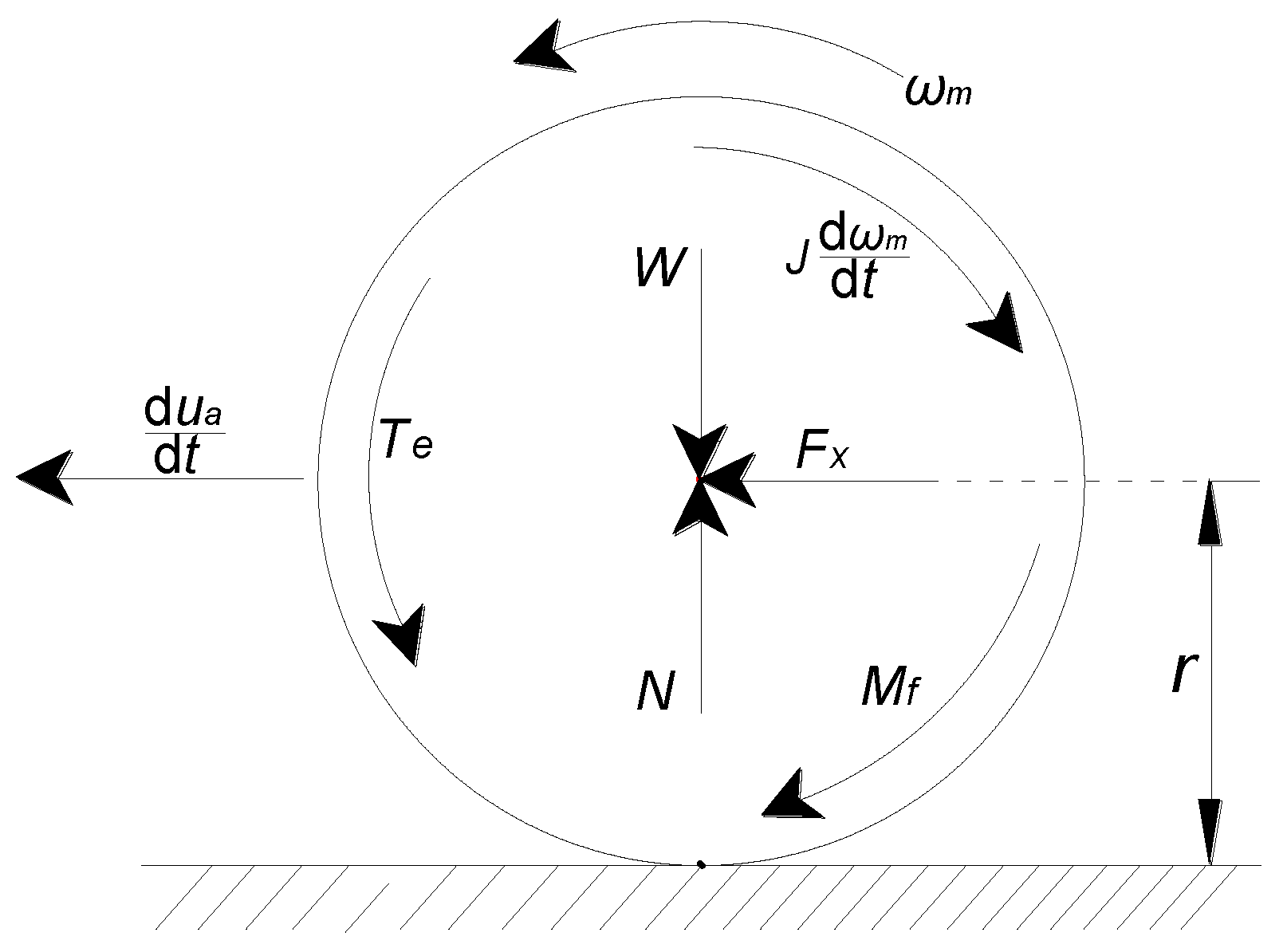
In MMS, the OSM driving force originates only from the electric wheels. To explore MMS control strategies, it is necessary to establish a theoretical model of the electric wheel. A force diagram of the electric wheel during acceleration assuming that tire deformation is small and can be ignored and the tire is rolling on a hard road is shown in Figure 3.

The force diagram in Figure 3 shows that the relationship between the electric wheel angular velocity and the longitudinal tire force is as follows:

$$F_x=\frac{1}{r}(T_e-B_m{\omega }_m-J\frac{\mathbf{d}{\omega }_m}{\mathbf{d}t}-M_f),$$

(5)

where F_x is the longitudinal tire force (N); r is the electric wheel radius (m); T_e is the electromagnetic torque of the motor (N·m); B_m is the viscous friction damping coefficient (N·m); ω_m is the electric wheel angular velocity (rad·s⁻¹); J is the moment of inertia (kg·m²); M_f is the rolling resistance moment (N·m); and t is time (s).

Based on the OSM structure, the angular velocities of the off-center arm and the electric wheel have the following relationship:

$${\omega }_m=K\omega ,$$

(6)

where K is a constant coefficient.

2.4. General Flexible Chassis Kinetic Model

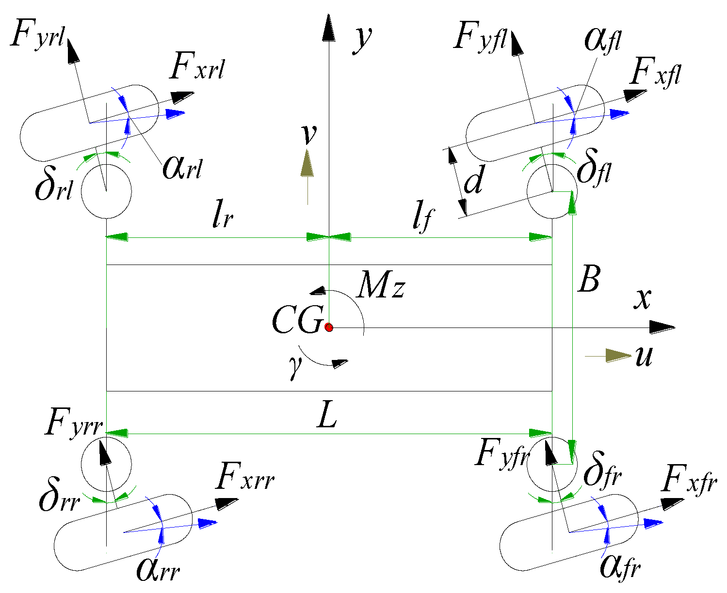
A simplified chassis dynamics model (Figure 4) is adopted to establish the FC MMS state equation. This study only considers the vehicle’s longitudinal motion (x-direction), lateral motion (y-direction), and yaw motion (rotation around the z-axis). It is also assumed that there is no suspension system effect or air resistance. Changes in vehicle longitudinal speed are ignored. The coordinate system of the model takes the centroid (CG) of the FC as the origin. The x-axis is the longitudinal direction of the FC and the y-axis is the lateral direction.

In the dynamic model, the kinetic equations for longitudinal, lateral, and yaw motion are expressed using Equations (7)–(9), respectively:

$$m(\dot{u}-v\gamma )={\displaystyle \sum _{i=1}^4(F_{xi}}\cos {\delta }_i-F_{yi}\sin {\delta }_i),$$

(7)

$$m(\dot{u}+v\gamma )={\displaystyle \sum _{i=1}^4(F_{xi}}\sin {\delta }_i+F_{yi}\cos {\delta }_i),$$

(8)

$$I\dot{\gamma }=M_Z,$$

(9)

where u is longitudinal speed, v is lateral speed, I is the moment of inertia of the FC, m is the mass of the FC, and i = 1(fl), 2(fr), 3(rl), 4(rr).

According to the linear tire model [33], the steering angle, side-slip angle, longitudinal speed, and lateral speed have the following relationship:

$$\tan ({\alpha }_i+{\delta }_i)=\frac{v_j}{u_j},$$

(10)

where α_i denotes a side-slip angle, v_j denotes longitudinal speed, and u_j denotes lateral speed (j = CM, IM, DM, SM).

The side-slip angle of each motion is calculated as:

$$\{\begin{array}{l}{\alpha }_{fl}={\delta }_{fl}-{\tan }^{-1}(\frac{v+l_f\gamma }{u-0.5B\gamma }),{\alpha }_{fr}={\delta }_{fr}-{\tan }^{-1}(\frac{v-l_f\gamma }{u-0.5B\gamma })\\ {\alpha }_{rl}={\delta }_{rl}-{\tan }^{-1}(\frac{v+l_r\gamma }{u+0.5B\gamma }),{\alpha }_{rr}={\delta }_{rr}-{\tan }^{-1}(\frac{v-l_r\gamma }{u+0.5B\gamma })\end{array}.$$

(11)

The tire side-slip angle generally is very small in normal driving. It can be assumed that there is a linear relationship between the tire side force and the side-slip angle of the FC. The relationship between tire side force F_y, side-slip angle α, and tire cornering stiffness C_α is then given by:

$$F_{yj}=-C_{\alpha j}{\alpha }_j.$$

(12)

Finally, the state equation of FC movement is derived as follows:

$$\begin{array}{l}\left[\begin{array}{l}\dot{v}\\ \dot{\gamma }\end{array}\right]=\left[\begin{array}{cc}-\frac{C_{\alpha fl}+C_{\alpha fr}+C_{\alpha rl}+C_{\alpha rr}}{mu}\hfill & \hfill \frac{l_r(C_{\alpha rl}-C_{\alpha rr})-l_f(C_{\alpha fl}-C_{\alpha fr})}{mu}-u\\ \frac{l_r(C_{\alpha rl}+C_{\alpha rr})-l_f(C_{\alpha fl}+C_{\alpha fr})}{Iu}& -\frac{l_f^2(C_{\alpha fl}-C_{\alpha fr})+l_r^2(C_{\alpha rl}-C_{\alpha rr})}{Iu}\hfill \end{array}\right]\left[\begin{array}{l}v\\ \gamma \end{array}\right]\\ +\left[\begin{array}{l}\frac{C_{\alpha fl}}{mu}\frac{C_{\alpha fr}}{mu}\frac{C_{\alpha rl}}{mu}\frac{C_{\alpha rr}}{mu}\\ \frac{l_f{C}_{\alpha fl}}{I}\frac{l_f{C}_{\alpha fr}}{I}\frac{l_f{C}_{\alpha rl}}{I}\frac{l_f{C}_{\alpha rr}}{I}\end{array}\right]\left[\begin{array}{l}{\delta }_{fl}\\ {\delta }_{fr}\\ {\delta }_{rl}\\ {\delta }_{rr}\end{array}\right]\end{array}$$

(13)

Similarly, based on the above derivation, the state equations for CM, IR, DM, and SM can be derived according to Equation (13) and will not be derived here again.

3. Control Strategy

3.1. Coupling Error Control Model

In the previous study, the distribution control method was adopted for MMS of the FC. The command signal was directly assigned to each OSM according to the desired angle of each mode. The steering angle tracking control of each OSM was implemented based on bridge circuit, but the coupling motion of four OSMs was not considered. This methodology is simple and easy to implement when the four OSMs are steering independently without restraining each other. In this study, a coupling control strategy is proposed. The CE of an off-center arm is obtained by comparing the angular velocity between two adjacent OSMs. Then, the CE of each OSM is compensated using the coupling control algorithm. Any changes in the angular velocity of an OSM will provide feedback to an adjacent OSM. All adjacent steering mechanisms are coupled in pairs, eventually forming a coupling loop. This study observes the effect of the proposed coupling control by comparing it with the distribution control method.

In the MMS process, the expected angular velocity of an off-center arm, ω_d, is the only input signal. However, the angular velocities of the off-center arms are different under different motion modes. In a motion mode, the proportional relationship between the angular velocities of all off-center arms is expressed as:

$$\frac{{\omega }_1}{{\eta }_1}=\frac{{\omega }_2}{{\eta }_2}=\cdots =\frac{{\omega }_n}{{\eta }_n},$$

(14)

where η_p is proportionality coefficient (p = 1, 2, …, n).

The kth off-center arm with the worst control performance is selected as a reference, and its proportionality coefficient is η_k. For convenience of synchronization error derivation, a normalized proportional coefficient ${\eta }_p^{*}$ is introduced:

$${\eta }_p^{*}=\frac{{\eta }_p}{{\eta }_k}=\frac{{\omega }_p}{{\omega }_k}.$$

(15)

In a control system with n OSMs, the angular velocity tracking error of OSM p is defined as

$$e_p={\omega }_p^{*}-{\omega }_p,$$

(16)

where ${\omega }_p^{*}={\eta }_p^{*}\cdot {\omega }_d$, and ω_d represents the demand angular velocity.

The synchronization error between any two adjacent OSMs is expressed using Equation (17). Synchronization control of all OSMs is achieved when ε_p = 0:

$${\epsilon }_p=\frac{{\omega }_p}{{\eta }_p^{*}}-\frac{{\omega }_{p+1}}{{\eta }_{p+1}^{*}}.$$

(17)

The dynamic characteristics of the OSM are described using:

$${\dot{\omega }}_p=\frac{1}{J_o}(T_e-T_s)-(\frac{B_o}{J_o}){\omega }_p,$$

(18)

where T_s is the load torque (N·m); B_o is the viscous friction damping coefficient of the OSM (N·m); and J_o denotes the OSM moment of inertia (kg·m²).

Equation (18) can be simplified as:

$${\dot{\omega }}_p=f-b{\omega }_p,$$

(19)

where f = (T_e − T_s)/J_o, b = B_o/J_o.

The CE of the pth OSM after compensation in coupling control is given as:

$$E_p=e_p-{\lambda }_p{\epsilon }_p,$$

(20)

where λ_p represents the synchronization error coefficient, e_p is the OSM tracking error, and ε_p is the OSM coupling error.

To achieve coupling control, E_p must be maintained at zero. According to Lyapunov’s direct method, a Lyapunov function can be constructed for a nonlinear differential equation to study its stabilization in a control system. To make E₁ zero, the Lyapunov function is used to judge the system stability. Similar to the studies of [34,35,36], taking the wheel 1 of the FC as an example, a Lyapunov function is constructed to judge the system stability, as shown by Equation (21):

$$V_1=\frac{E_1^2}{2}>0.$$

(21)

If Equation (22) exists and Equation (23) is true, the system is stable when E₁ approaches zero:

$${\dot{E}}_1=-c_1{E}_1(c_1>0),$$

(22)

$${\dot{V}}_1=E{\dot{E}}_1=-c_1{E}_1^2<0.$$

(23)

Combining Equations (17), (19), and (20) allows the following equation to be derived:

$${\dot{E}}_1={\dot{e}}_1-{\lambda }_1{\dot{\epsilon }}_1={\eta }_1^{*}{\dot{\omega }}_d-{\dot{\omega }}_1-{\lambda }_1\frac{{\dot{\omega }}_1}{{\eta }_1^{*}}+{\lambda }_1\frac{{\dot{\omega }}_2}{{\eta }_2^{*}},$$

(24)

$${\dot{E}}_1={\eta }_1^{*}{\dot{\omega }}_d-f_1+b_1{\omega }_1-{\lambda }_1\frac{f_1}{{\eta }_1^{*}}+{\lambda }_1\frac{f_2}{{\eta }_2^{*}}+{\lambda }_1\frac{b_1{\omega }_1}{{\eta }_1^{*}}-{\lambda }_1\frac{b_2{\omega }_2}{{\eta }_2^{*}}$$

(25)

$${\dot{E}}_1=-b_1{\lambda }_1{\epsilon }_1-\left(b_1+b_1{\lambda }_1+b_2{\lambda }_1\right)e_1+{\mu }_1,$$

(26)

where ${\mu }_1={\eta }_1^{*}{\dot{\omega }}_d+b_1{\omega }_d-f_1+b_1{\lambda }_1{\epsilon }_1-{\lambda }_1{\dot{\epsilon }}_1+\left(b_1{\lambda }_1+b_2{\lambda }_1\right)e_1$, and μ₁ is the control function of the left front off-center steering shaft.

If ${\dot{E}}_1=-c{E}_1$, then Equation (27) is true:

$$-b_1{\lambda }_1{\epsilon }_1-\left(b_1+b_1{\lambda }_1\right)e_1+{\mu }_1=-c_1\left(e_1-{\lambda }_1{\epsilon }_1\right),$$

(27)

where

$${\mu }_1=\left(c_1+b_1\right){\lambda }_1{\epsilon }_1+\left(b_1-c_1+b_1{\lambda }_1+b_2{\lambda }_1\right)e_1.$$

(28)

For any positive real number c₁, μ₁ can be constructed such that E₁ approaches zero. Therefore, we can construct Equation (28) to make E₁→0. Similarly, μ_i can be constructed to make E_i→0. Based on the converse derivation of Equation (28), it also can be found that, if Equation (28) is established, then Equation (22) can be guaranteed. As one of the control parameters, c₁ will affect the regulation time and overshoot of the control system. Through pre-research simulation, it was found that, if c₁ is too small, the adjustment time of the system will increase, and, if c₁ is too large, the overshoot will increase.

3.2. Fuzzy PID Coupling Error Control Strategy

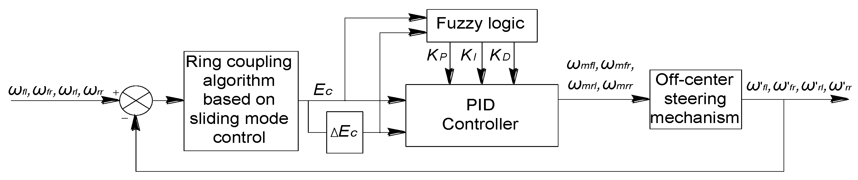
PID controllers are frequently used for vehicle control. However, satisfactory results are difficult to achieve when working conditions and control parameters change. In contrast, a fuzzy logic controller (FLC) does not require a precise mathematical model of the system. This FLC property guarantees stable system operation even if the control parameters and conditions undergo dynamic change [37]. The fuzzy method has the advantages of keeping a simple control structure and avoiding costly sensor use [28,38]. In this paper, the angular velocity CE is adjusted via control of the in-wheel motor speed. The speed of the in-wheel motor is controlled according to the CE and its change rate. Additional control of the in-wheel motor speed is needed to avoid the interference of multiple random factors. Therefore, developing a controller based on fuzzy logic is an attractive choice, and a fuzzy PID controller was designed for CE control of MMS.

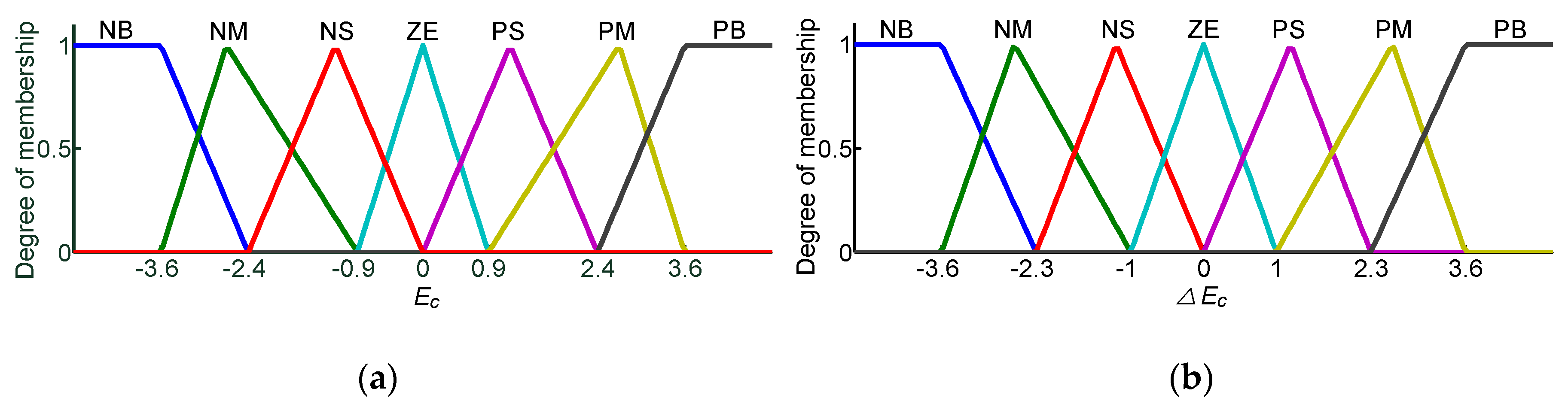
The CE and its change rate are the two key parameters in the process of synchronous motion adjustment. Therefore, the CE and its change rate are used as fuzzy controller inputs E_c and ΔE_c, and the two-dimensional fuzzy controller is the most suitable type. The fuzzy PID controller structure is shown in Figure 5. Seven fuzzy linguistic terms are adopted for both inputs and outputs: negative big (NB), negative medium (NM), negative small (NS), zero (Z), positive small (PS), positive medium (PM), and positive big (PB). Some basic fuzzy PID control processes are described as follows. When E_c and ΔE_c are small, larger K_P and K_I and proper K_D should be adopted compared with current parameters, in order to stabilize the steering system. When E_c and ΔE_c are medium-sized, smaller K_P and proper K_I and K_D are used to reduce steering angle overshoot. When E_c and ΔE_c are large, larger K_P and smaller K_I and K_D are used to avoid excessive overshoot and expedite the steering response. The membership functions were fine-tuned experimentally based on human experiences of vehicle operation until the system performed acceptably [39]. Figure 6 shows the membership function curves. The fuzzy rules are shown in

Table 1. Fuzzy rules for ∆K_P, ∆K_I, and ∆K_D.

∆Kp/∆Ki/∆Kd					∆Ec
		NB	NM	NS	Z	PS	PM	PB
	NB	PB/NB/PS	PB/NB/NS	PM/NM/NB	PS/NM/NB	PS/NS/NB	Z/Z/NM	Z/Z/PS
	NM	PB/NB/PS	PM/NB/NS	PM/NM/NB	PS/NS/NM	PS/NS/NM	Z/Z/NS	NS/Z/Z
	NS	PM/NM/Z	PM/NM/NS	PM/NS/NM	PS/NS/NM	Z/Z/NS	NS/PS/NS	NS/PS/Z
Ec	Z	PM/NM/Z	PM/NM/NS	PS/NS/NS	Z/Z/NS	NS/PS/NS	NM/PS/NS	NM/PM/Z
	PS	PS/NS/Z	PS/NS/Z	Z/Z/Z	NS/PS/Z	NS/PS/Z	NM/PM/Z	NM/PM/Z
	PM	PS/Z/PB	Z/Z/NS	NS/PS/PS	NM/PM/PS	NM/PM/PS	NM/PM/PS	NB/PB/PB
	PB	Z/Z/PB	Z/Z/PM	NM/PS/PM	NM/PM/PM	NM/PB/PS	NB/PB/PS	NB/PB/PB

. Exact changes in the PID parameters are calculated using the center-of-area method.

3.3. Off-Center Arm Steering Angle Tracking Error Control Strategy

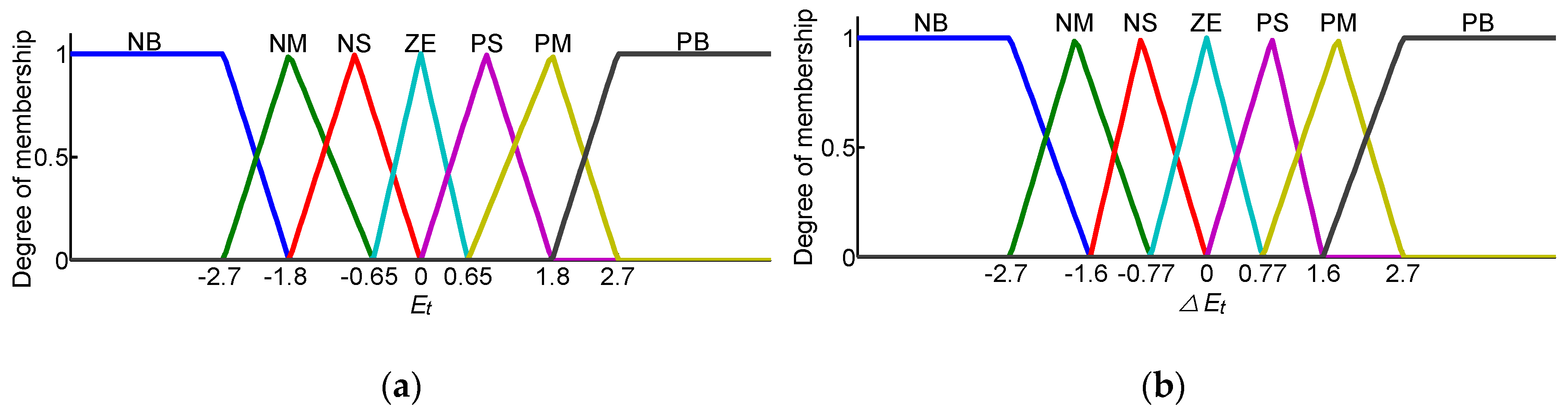
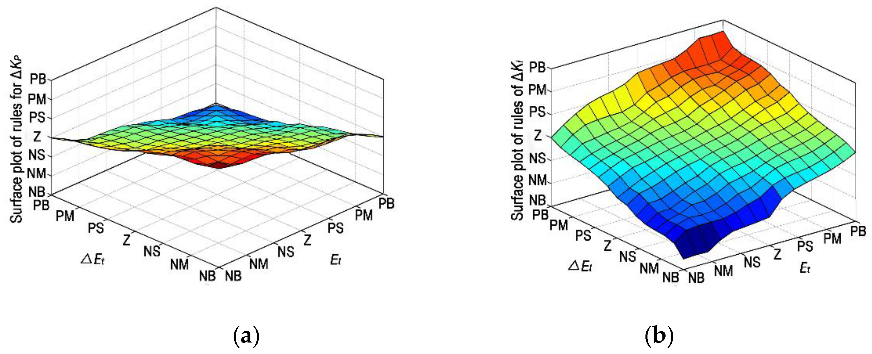
In previous research, bridge circuits [40] were used for off-center arm angle tracking control. However, the bridge circuit-based control system exhibits large steady-state errors. To solve this problem, the fuzzy PI control method is employed. It is also possible to use PID for steering angle tracking control, but its parameter adjustment is more complex than PI control [41,42]. From the previous test, PI control was sufficient for steering angle tracking control. Therefore, a fuzzy PI controller was employed to improve processing efficiency. Fast steering response can be achieved and angle error can be reduced via the auxiliary PI algorithm and self-tuning of the proportional and integral coefficients. The fuzzy method still uses a two-dimensional fuzzy controller and the inputs are the errors of the steering angles and the error rate (E_t and ΔE_t). The outputs are the K_P and K_I corrections for PI control. In this controller, the seven fuzzy linguistic terms are introduced to describe the input and output variable values: input variable 1: E_t∈{NB, NM, NS, Z, PS, PM, PB}; input variable 2: ΔE_t∈{NB, NM, NS, Z, PS, PM, PB}; output 1: K_P∈{NB, NM, NS, Z, PS, PM, PB}; and output 2: K_I∈{NB, NM, NS, Z, PS, PM, PB}. The membership function curves are shown in Figure 7. The membership functions were also fine-tuned experimentally. Figure 8 shows a surface plot of the input and the output fuzzy logic variables of ∆K_P and ∆K_I.

4. Simulation and Analysis

4.1. Simulation Parameters

To assess the feasibility of the proposed control strategy, MATLAB/Simulink (R2014a, MathWorks Company, Natick, MA, USA, 2014) simulations of coupling and distribution control were performed. The simulation model is composed primarily of an angle distribution planner, a fuzzy PID controller, and a fuzzy PI controller for each wheel. The main FC parameters used in the simulations are shown in

Table 2. Main FC motion mode switching (MMS) simulation parameters.

Parameter	Description	Value	Parameter	Description	Value
m	Mass of flexible chassis	202.6 kg	d	Offset distance	253 mm
h	Ground clearance	300 mm	I	Yaw moment of inertia	1275 kg·m2
L	Distance between front and rear off-center shafts	1210.6 mm	Bo	Viscous friction damping coefficient	0.09 N·m /(rad·s−1)
B	Distance between left and right off-center shafts	610.5 mm	Bm	Viscous friction damping coefficient	0.07 N·m·s/rad
P	Rated power	500W	Te	Electric wheel output torque	35.4 N·m
J	Moment of inertia	0.0007 kg·m2	Cαfl	Tire cornering stiffness	4600 N·rad−1
Vr	Rated voltage	48 V	Cαfr	Tire cornering stiffness	4600 N·rad−1
ωmr	Rated rotation speed	500 r·min−1	Cαrl	Tire cornering stiffness	4600 N·rad−1
r	Tire radius	280 mm	Cαrr	Tire cornering stiffness	4600 N·rad−1
Tf	Tire damping	500 N/m·s−1	K	Constant coefficient	2.3
Tr	Rolling resistance coefficient	0.012	Jo	Moment of inertia	0.0011 kg·m2

.

The CE is the key index that characterize the coupling control performance of the four OSMs. Longitudinal and lateral acceleration are the main indicators used to determine stability during MMS. Changes in the steering angles and angular velocities of the four OSMs also must be detected. Thus, the simulations included three parts: the steering responses of four off-center arms, the CE performance, and the longitudinal and lateral acceleration changes under distribution and coupling control. The feasibility of the proposed method can be determined by comparing these two control methods.

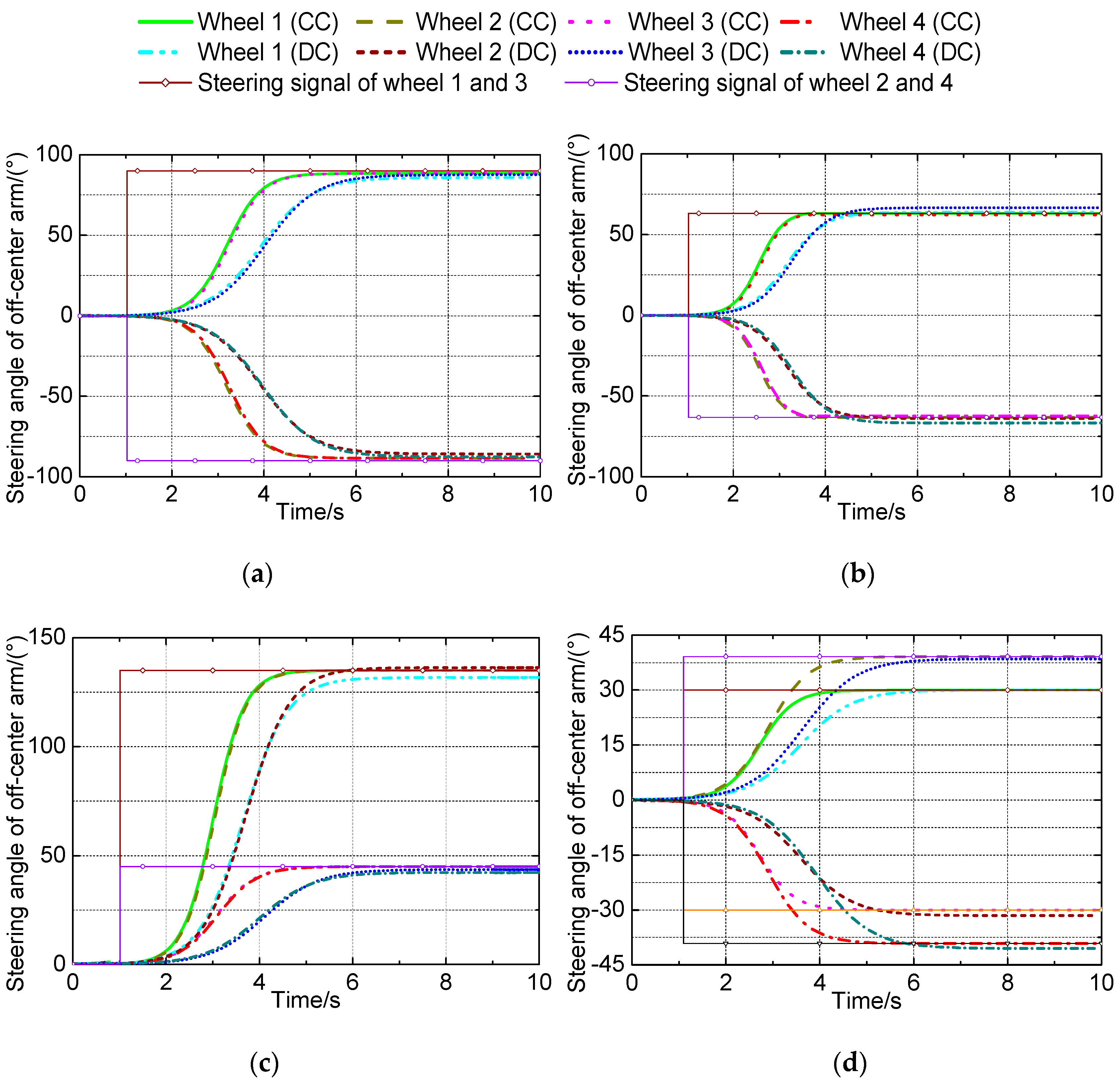
According to the analysis in Section 2.2, the target steering angle in any off-center arm is 90° during CM switching and 63° during IR switching. During DM switching, the target steering angle of off-center arms 1 and 3 is set to 45°, while off-center arms 2 and 4 are set to 135°. During SM switching, the target steering angles of off-center arms 1 and 3 is 30°, while arms 2 and 4 use 39° based on Ackermann steering geometry.

4.2. Simulation Results

MMS steering angle simulation results with distribution and coupling control are shown in Figure 9. In CM, IR, DM, and SM, the switching time in coupling control is shorter than that used in distribution control. The mode switching times for CM, IR, DM, and SM are respectively 4.9 s, 3.4 s, 3.3 s, and 4.2 s, respectively, under coupling control. Under distribution control, the mode switching times are 6.1 s, 4.8 s, 5.1 s, and 5.5 s, respectively. Of these four motions, the IR mode switching time is the shortest whether coupling or distribution control is used. This is primarily due to the small, symmetrical rotation angles of the four OSMs. The average steering angle errors of the four OSMs are 0.4°, 0.3°, 0.6°, and 0.6° for CM, IR, DM, and SM, respectively, under coupling control. Under distribution control, their respective errors are 1.4°, 1.1°, 1.7°, and 1.6°.

In addition, Figure 9d shows that the relationships between the two front and two rear wheels are better maintained under coupling control than under distribution control. The results demonstrate that there is good steering angle symmetry and uniformity among the four OSMs during coupling control mode switching. Overall, the four OSM steering angles exhibit better synchronization under the proposed control methodology than under distribution control.

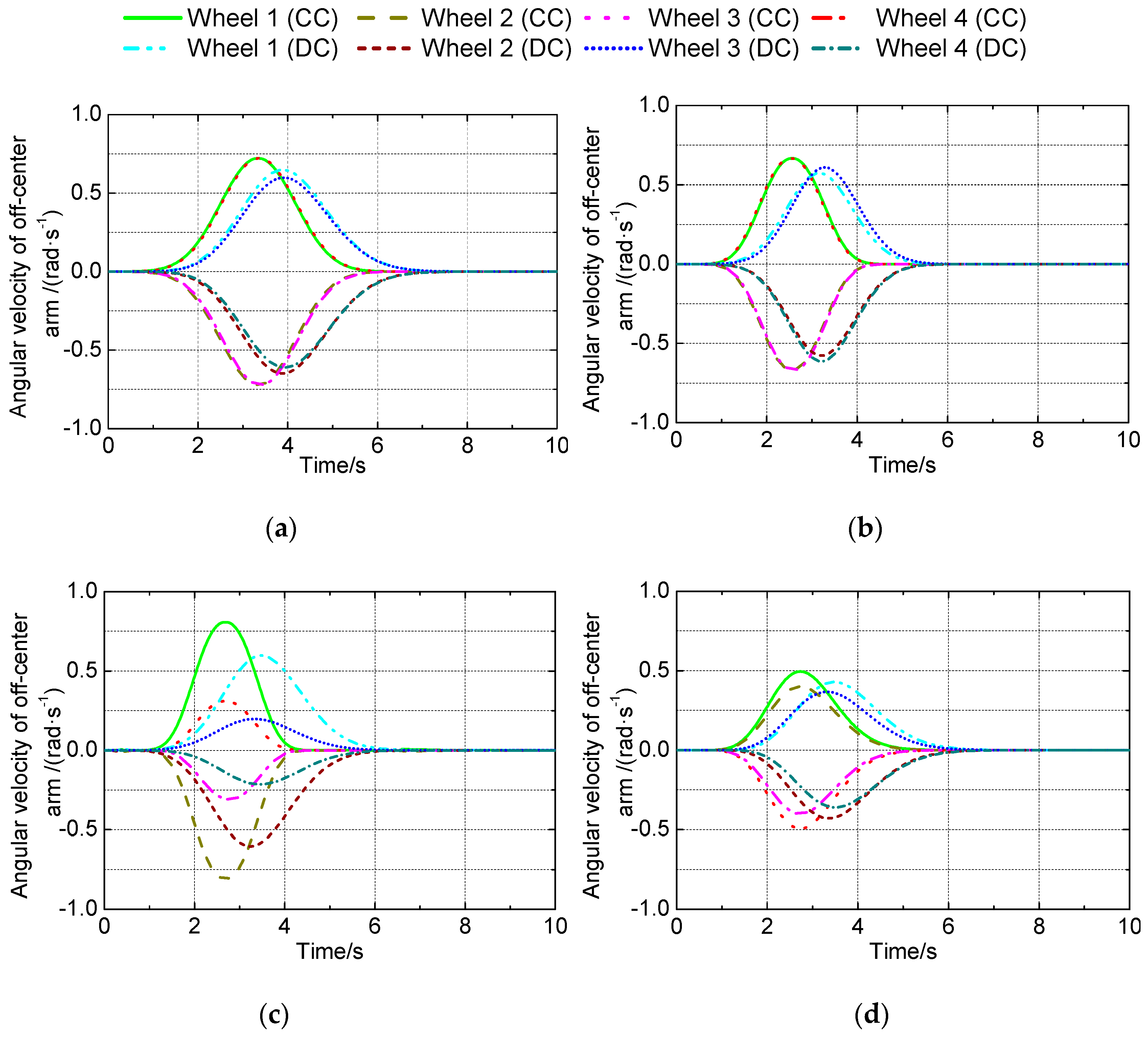
Angular velocity distribution and coupling control MMS simulation results are shown in Figure 10. In all motion modes, the angular velocity first increases and then decreases smoothly. All modes exhibit maximum angular velocity. Under distribution control, the angular velocity responses are slower than under coupling control. The maximum angular velocities are all smaller as well. The maximum angular velocities of the four OSMs do not maintain good symmetry under distribution control. For example, in CM, the maximum angular velocities are all nearly 0.74 rad·s⁻¹ but only 0.63 rad·s⁻¹, 0.61 rad·s⁻¹, 0.60 rad·s⁻¹, and 0.62 rad·s⁻¹ for the left front, right front, left rear, and right rear OSMs, respectively, under distribution control. Results from the other three motion modes are similar to those from CM. The CM, IR, and SM time differences are all above 1 s. The biggest mode switching time difference between coupling and distribution control occurs during DM. The time difference for this motion can reach approximately 2 s. One can speculate that the angular velocities of the four OSMs under coupling control show better synchronicity than those under the proposed control methodology.

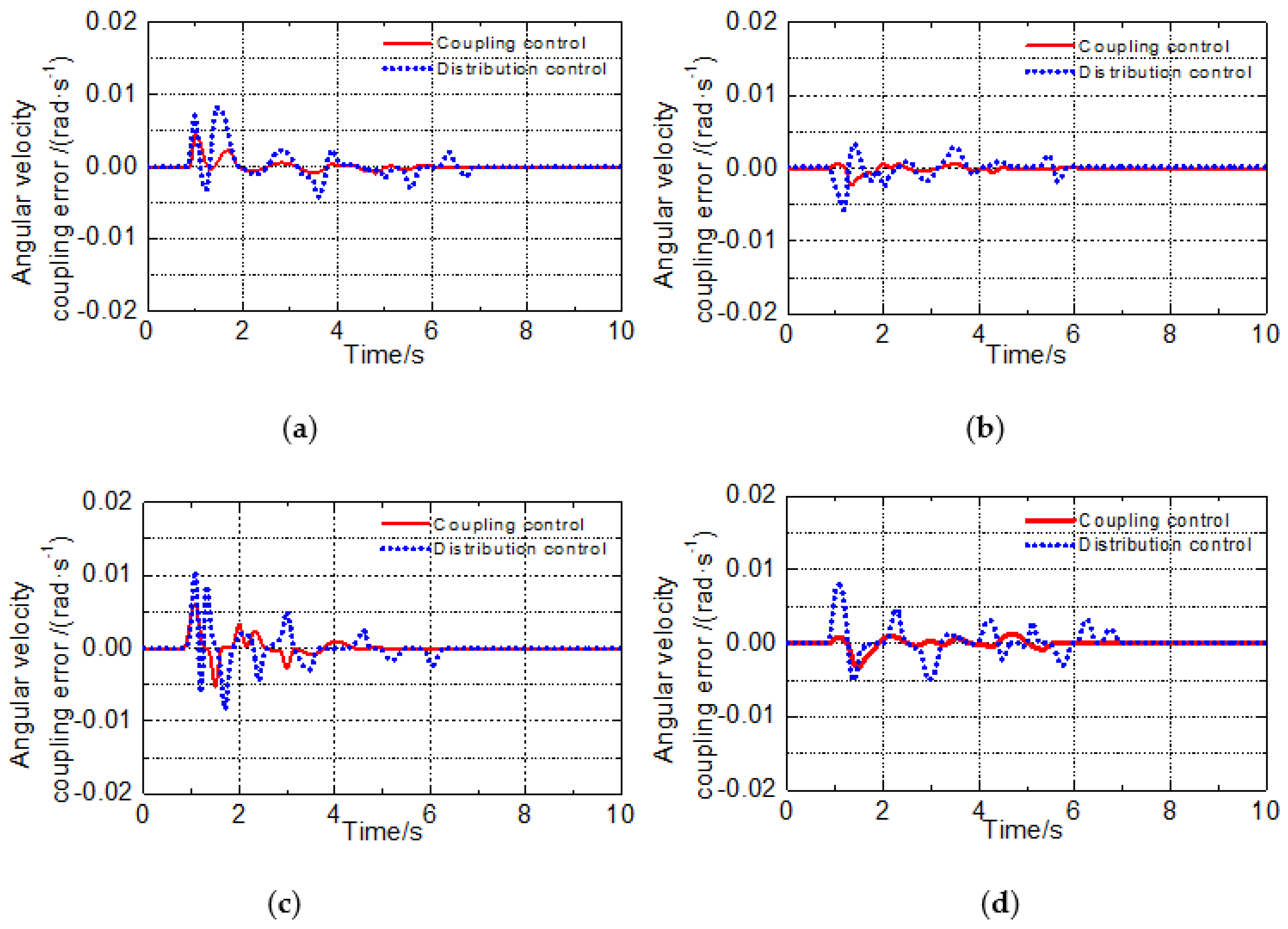
The OSM CE curves for all motion modes are shown in Figure 11. We take the CE between wheel 1 and wheel 2 as an example for analysis. Obviously, the CEs are greater under distribution control than under coupling control. The respective absolute maximum angular velocity CEs during CM, IR, DM, and SM are 0.008 rad·s⁻¹, 0.006 rad·s⁻¹, 0.011 rad·s⁻¹, and 0.007 rad·s⁻¹ under distribution control. The respective average CEs are 0.002 rad·s⁻¹, 0.001 rad·s⁻¹, 0.003 rad·s⁻¹, and 0.003 rad·s⁻¹ for these four motions. In coupling tests, the maximum CEs are 0.004 rad·s⁻¹, 0.002 rad·s⁻¹, 0.006 rad·s⁻¹, and 0.003 rad·s⁻¹, respectively, and the average CEs are 0.0008 rad·s⁻¹, 0.0004 rad·s⁻¹, 0.001 rad·s⁻¹, and 0.0009 rad·s⁻¹, respectively. Clearly, the CEs change randomly throughout MMS during distribution control tests. In coupling control tests, the initial errors are somewhat large but gradually approach zero in later stages. This indicates that the coupling algorithm plays a role in MMS. The CE is greatest during DM regardless of which control method is used. This may be caused by the asymmetric kinematic characteristics and wide steering angles used by off-center arms 2 and 4 during this motion. Overall, the CE performance improves substantially under the proposed control methodology.

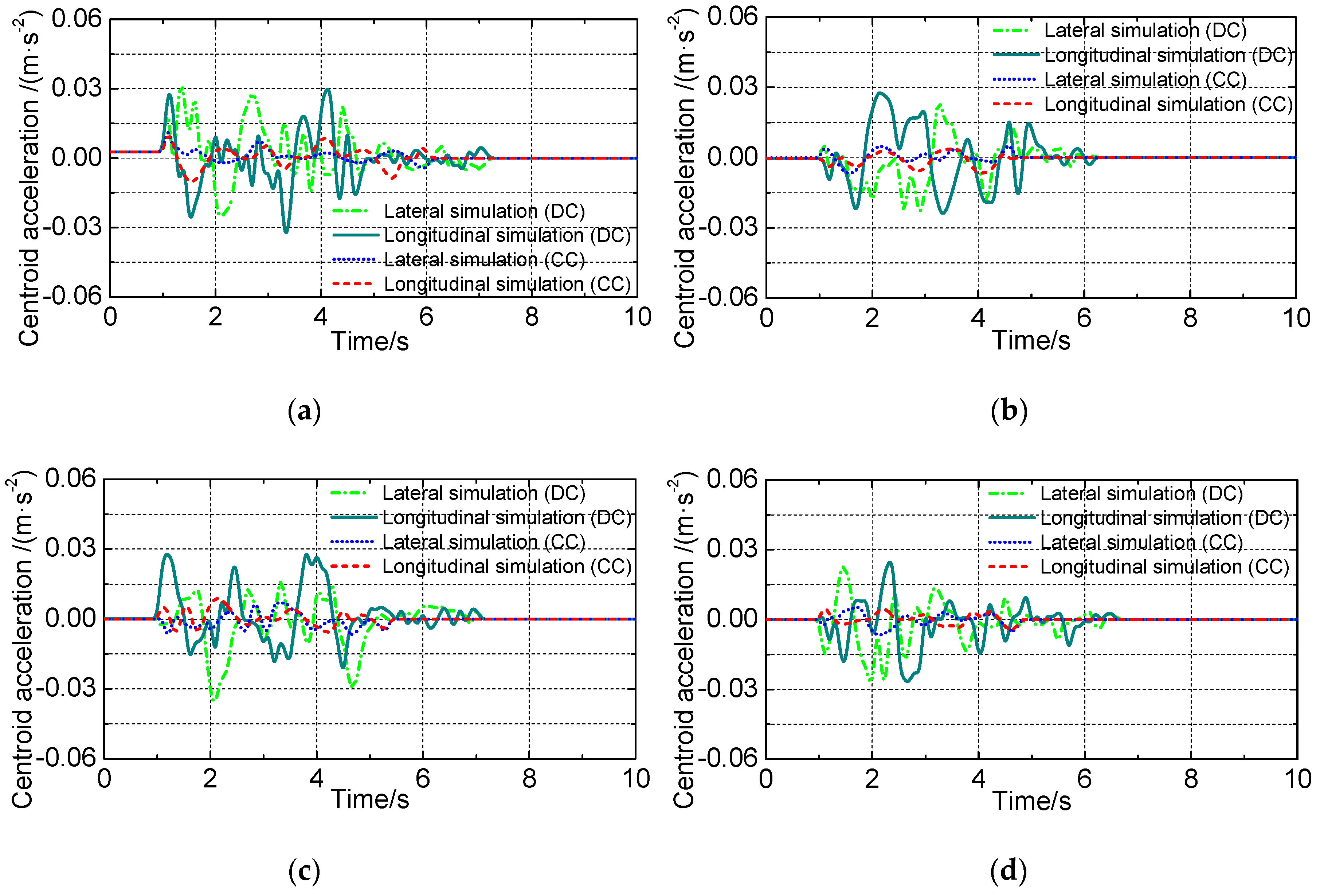
Figure 12 shows simulated mode switching longitudinal and lateral acceleration changes. In all motion modes, acceleration values are greater than simulation values and fluctuations occur. Meanwhile, acceleration is smaller under coupling control than under distribution control. In CM mode switching, the maximum absolute longitudinal acceleration rates under coupling control and distribution control are −0.033 m·s⁻² and −0.011 m·s⁻², respectively. In contrast, the maximum absolute lateral acceleration rates under coupling and distribution control are 0.031 m·s⁻² and 0.010 m·s⁻², respectively. The four values in the above order are 0.028 m·s⁻², −0.008 m·s⁻², −0.023 m·s⁻², and −0.006 m·s⁻² during IR mode switching, 0.029 m·s⁻², 0.008 m·s⁻², −0.035 m·s⁻², and 0.007 m·s⁻² during DM mode switching, and −0.028 m·s⁻², 0.004 m·s⁻², 0.028 m·s⁻², and −0.006 m·s⁻² during SM mode switching. From these results, we can see that the longitudinal and lateral disturbances are smaller under coupling control than under conventional distribution control. The maximum CE reduction reaches 50%. Therefore, MMS occurs with better stability under coupling control. This further demonstrates that the method proposed in this study is feasible and effective.

5. Experimental Verification

5.1. Experiment Equipment and Method

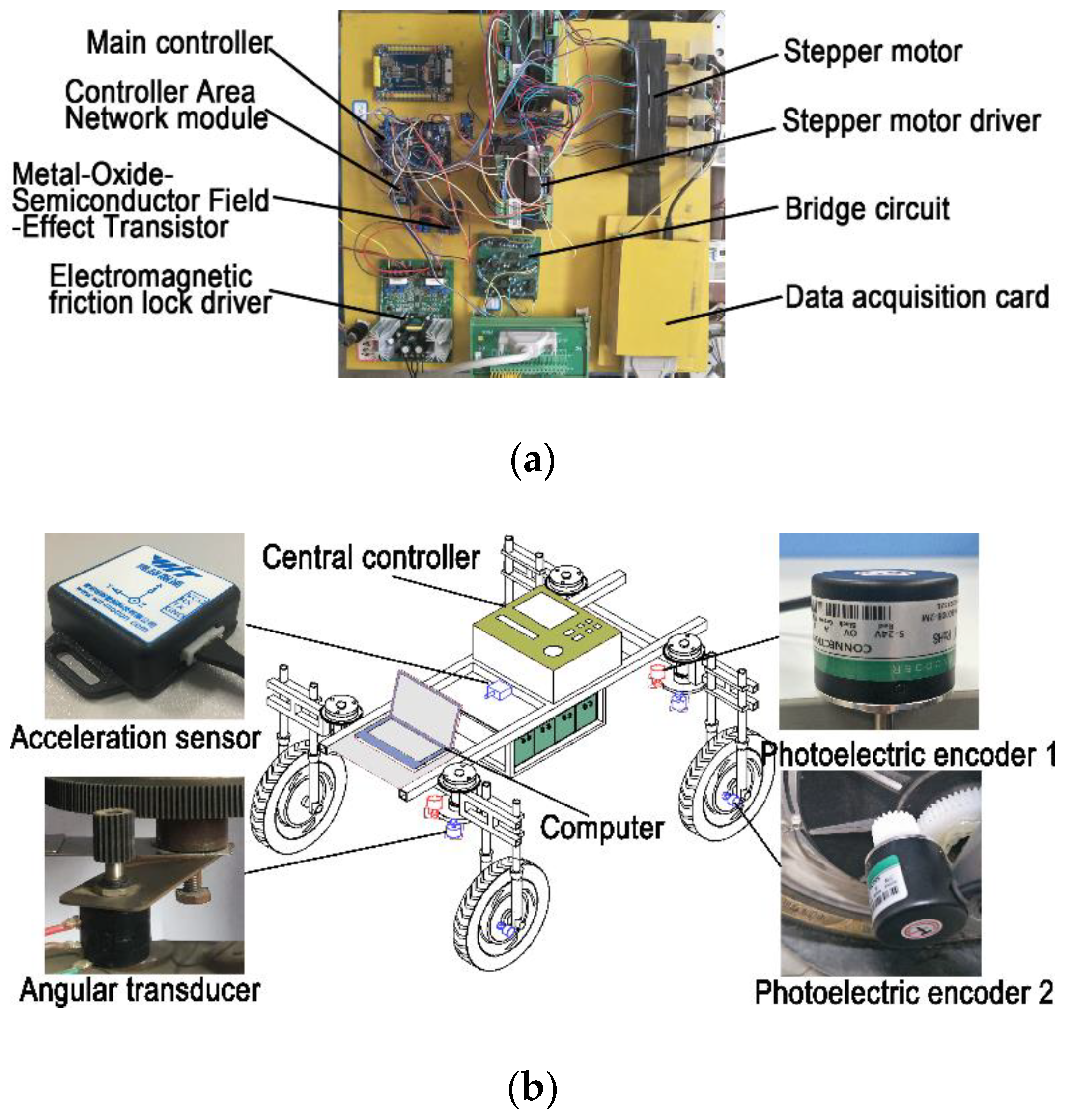
To further verify the effectiveness of the control strategy, the chassis system model was loaded from MATLAB into the MicroAutoBox real-time system. The embedded ECUs (Electronic Control Units) were implemented on STM32 units in order to perform tests on hard pavement. The control panel is shown in Figure 13a. The controller mainly included single-chip modules (STM32F103ZET6, STMicroelectronics, Geneva, Switzerland), stepper motors (YH42BYGH47-401A, Microstep, Bratislava, Slovakia) and their drivers, bridge circuit modules, and accessory circuits. Figure 13b shows the detailed configuration of the FC used for test. A photoelectric encoder (GTS06-OC-RA1000B-2M, pulse: 1000; Kasei Electronics Ltd., Tokyo, Japan) was used to acquire the speeds of in-wheel motors. The off-center arm steering angles were measured using a multi-turn potentiometer (22HP-10, 0–5 kΩ; Sakae Company, Tokyo, Japan). Acceleration sensors (WT61C232, Wit Technology Company, Dublin, Ireland) were used to detect the longitudinal and lateral FC acceleration rates. The duration of MMS was calculated by the clock integrated into the data acquisition equipment, which included a data acquisition card (USB7648B, Beijing Zhongtai Research Ltd., Beijing, China) and an industrial personal computer (610H, Advantech Technology Corporation, Beijing, China).

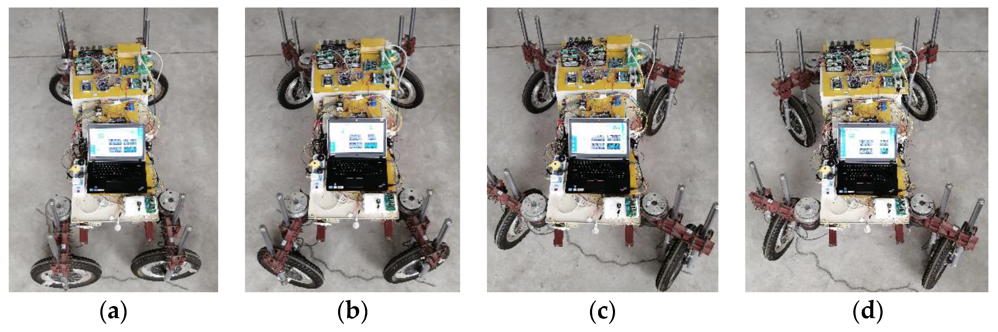
The FC MMS tests were performed as follows. First, we confirmed that all parts of the FC worked correctly. This included the mechanical connections, control lines, power supply lines, data acquisition system, etc. Second, we activated the data acquisition system and started CM mode switching under distribution control. After MMS was complete, we stopped saving data and restored the FC to its original state. Similar tests were performed using the coupling control method proposed in this study. Next, we used the method described above to conduct IR, DM, and SM MMS tests. Finally, we deactivated the controller, electric wheel power supply, and overall power supply in turn, and put the FC in standby mode. The tests were conducted on hard pavement on the north campus of Northwest A&F University. Images from various MMS tests are shown in Figure 14.

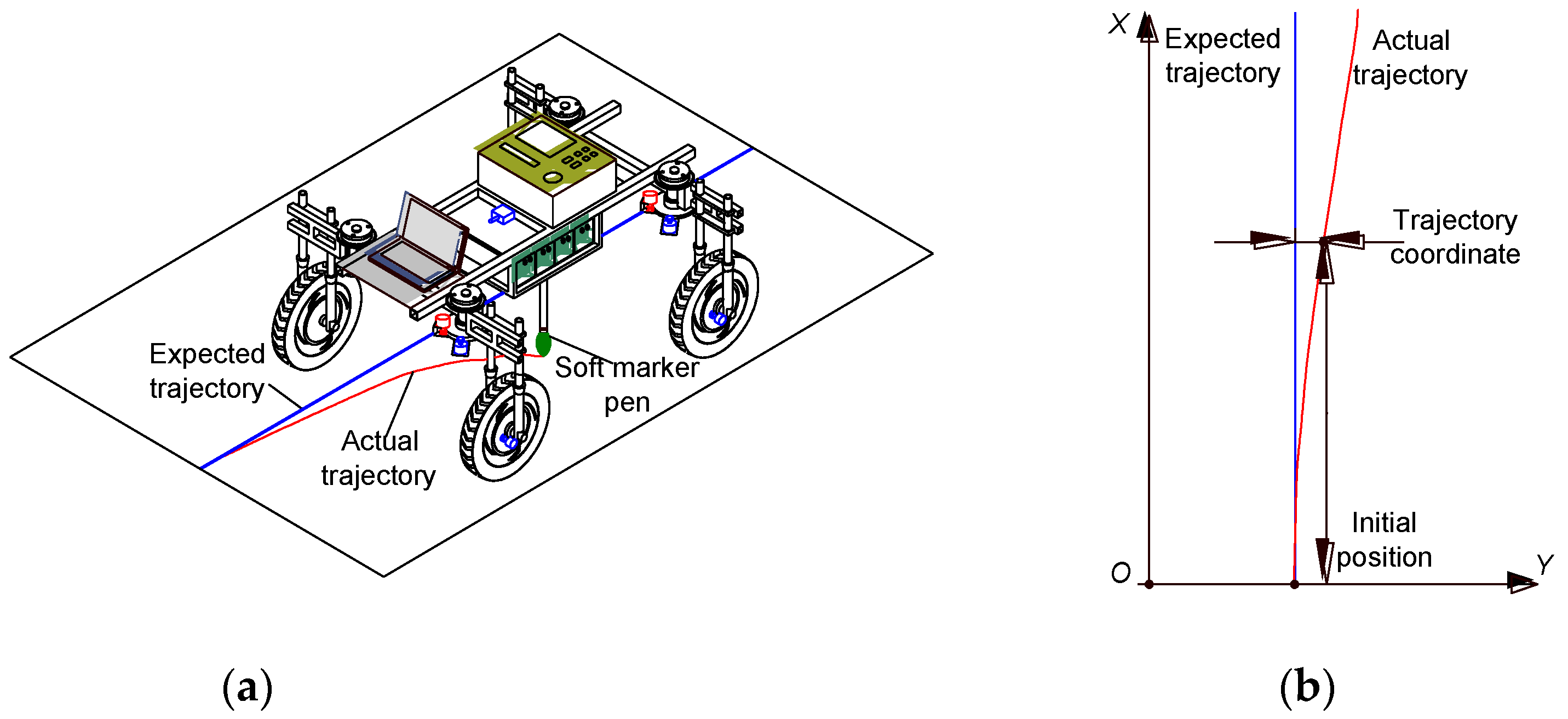
To further observe the effect of the proposed controller, we also tested the trajectory of the FC centroid. In this test, a soft marker pen fixed on the frame was used to obtain the trajectory of the FC (Figure 15a). The test was conducted when the FC moved with fixed posture after MMS was completed at the initial position (Figure 15b). The soft marker pen has a slight contact with the ground and the driving resistance of the FC was not affected by this pen. We created a coordinate system on the ground (Figure 15b). Through measuring the trajectory coordinate, the path behavior of the FC can be obtained.

5.2. Analysis of Results

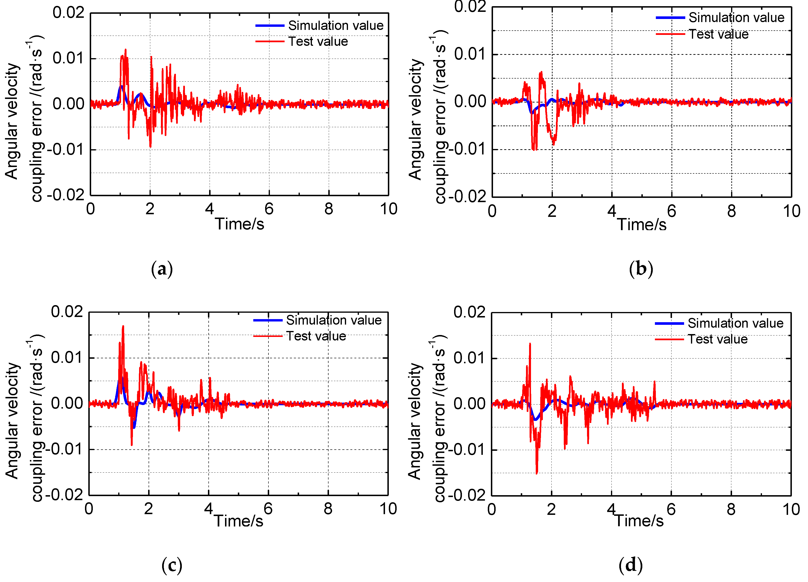
The CE test results are presented in Figure 16. The CE between wheel 1 and wheel 2 is still analyzed as an example. All of the experimental CEs are greater than those that were simulated CEs. The maximum experimental CE absolute values are 0.012 rad·s⁻¹, 0.01 rad·s⁻¹, 0.017 rad·s⁻¹, and 0.015 rad·s⁻¹ for CM, IR, DM, and CM mode switching, respectively. Although the experimental and simulated values are different, the CE change trends are consistent. In particular, large CE fluctuations occur as the MMS tests start. These gradually decay until they approach zero. Obviously, the proposed controller plays a role in MMS and the CEs are well controlled. These results prove that the proposed control method is effective.

The maximum and average acceleration rates are the main values used to evaluate longitudinal and lateral motion trends. Therefore, the results also focus on these two indices.

Table 3. Longitudinal and lateral acceleration of the flexible chassis centroid.

Motion Types	Longitudinal Acceleration		Lateral Acceleration
	Maximum Value/(m·s−2)	Average Value/(m·s−2)	Maximum Value/(m·s−2)	Average Value/(m·s−2)
Cross motion	0.057	0.007	0.056	0.005
In-place rotation	0.045	0.005	0.052	0.006
Diagonal motion	0.062	0.009	0.064	0.007
Steering motion	0.075	0.008	0.063	0.008

shows the longitudinal and lateral acceleration test results. As with the CEs, the experimental maximum absolute acceleration rates all exceed their simulated values, but are all in an acceptable range. The average absolute values are all quite small at approximately 9 to 12% of the maximum absolute value in most tests. This indicates that the changes in longitudinal and lateral FC directions are not notable. This shows that the proposed methodology can effectively guarantee FC stability during MMS.

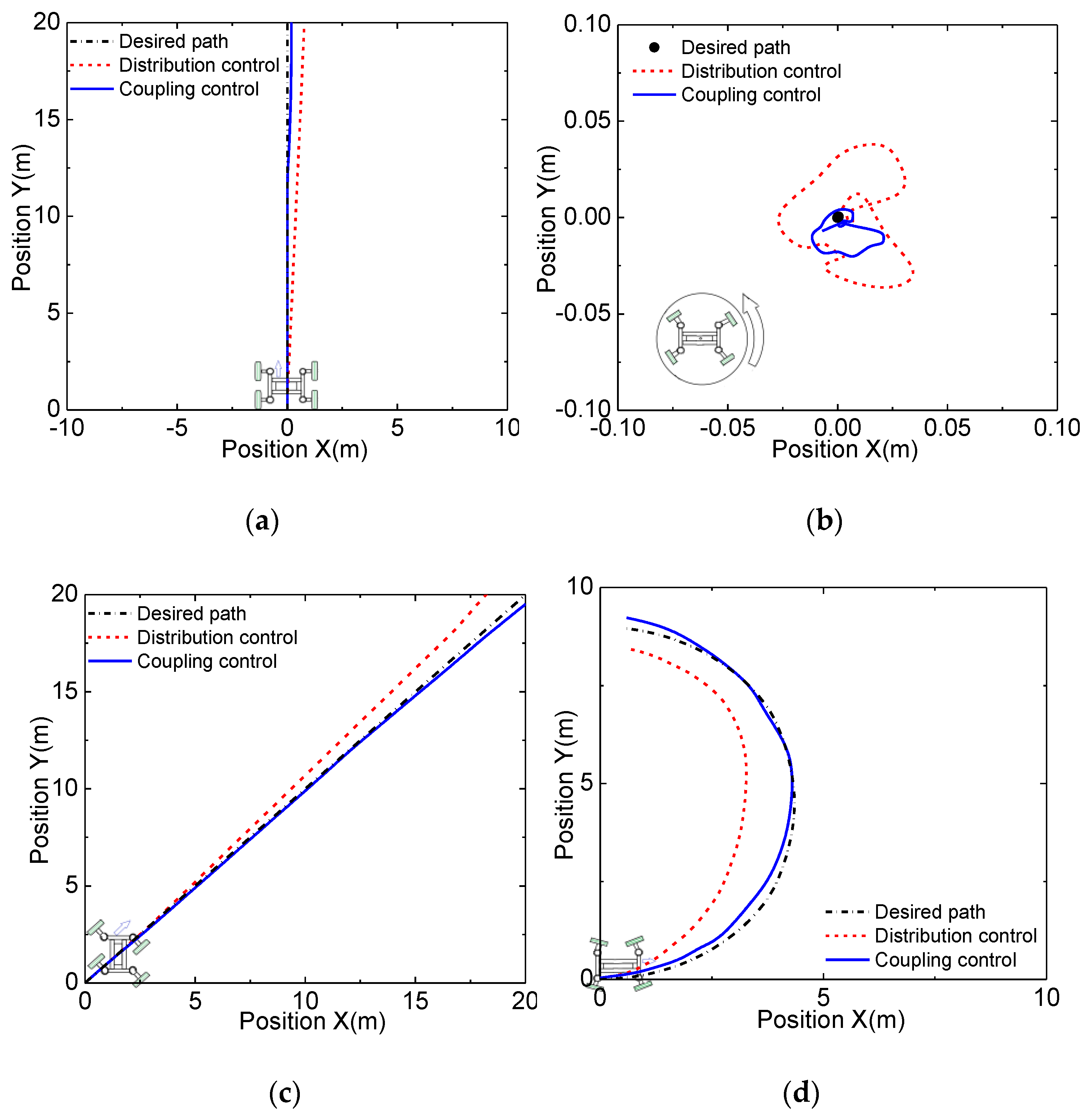
Figure 17 shows the centroid trajectory under distribution control and coupling control when the FC is moved in a fixed posture. Under the coupling control, the trajectory of the FC is more consistent with the expected trajectory. For the CM and DM process, the trajectory deviates early under distribution control. As the displacement increases, the trajectory deviation becomes more serious. In the coupling control, the trajectory does not shift slightly until the FC moves a large distance. In the IR process, the trajectory under distribution control is farther away from the desired center than coupling control. During the SM process, the trajectory deviates most from the expected path under distribution control. These results indicate that, under coupled control, the MMS effect is better, and the mode switching accuracy is higher than the distribution control.

6. Conclusions

This study presents a flexible chassis coupling control methodology designed to reduce coupling errors and improve motion mode switching stability and handling performance. A coupling error model was established for linkage control of an off-center steering mechanism based coupling control, and Lyapunov stability theory. A fuzzy PID controller was designed to compensate for the coupling error and a fuzzy PI method was employed to reduce off-center steering mechanism tracking errors as well. The proposed control methodology was examined by simulation and validated experimentally on hard pavement. Compared to the conventional distribution control method, the proposed approach could effectively reduce coupling errors and guarantee MMS control stability while substantially shortening response times. The coupling control method proposed in this study demonstrated better effectiveness and feasibility than distribution control. The results of the study show that the DM and SM MMS performance with regard to coupling error was not as good as the CM and IR performance. Thus, we should pay attention to the reasons for this performance difference. It is important to devise a strategy to improve FC MMS control.

References

- Lang, J.; Tian, J.; Zhou, Y.; Li, K.; Chen, D.; Huang, Q.; Xing, X.; Zhang, Y.; Chen, S. A high temporal-spatial resolution air pollutant emission inventory for agricultural machinery in China. J. Clean. Prod. 2018, 183, 1110–1120. [Google Scholar] [CrossRef]
- Ko, M.H.; Ryuh, B.S.; Kim, K.C.; Suprem, A.; Mahalik, N.P. Autonomous greenhouse mobile robot driving strategies from system integration perspective: Review and application. IEEE/ASME Trans. Mechatron. 2015, 20, 1705–1716. [Google Scholar] [CrossRef]
- Lovarelli, D.; Bacenetti, J. Exhaust gases emissions from agricultural tractors: State of the art and future perspectives for machinery operators. Biosyst. Eng. 2019, 186, 204–213. [Google Scholar] [CrossRef]
- Gonzalez-De-Soto, M.; Emmi, L.; Benavides, C.; Garcia, I.; Gonzalez-de-Santos, P. Reducing air pollution with hybrid-powered robotic tractors for precision agriculture. Biosyst. Eng. 2016, 143, 79–94. [Google Scholar] [CrossRef]
- Bechar, A.; Vigneault, C. Agricultural robots for field operations: Concepts and components. Biosyst. Eng. 2016, 149, 94–111. [Google Scholar] [CrossRef]
- Chang, C.; Song, G.; Lin, K.M. Two-stage guidance control scheme for high-precision straight-line navigation of a four-wheeled planting robot in a greenhouse. Trans. ASABE 2016, 59, 1193–1204. [Google Scholar] [CrossRef]
- Reina, G.; Milella, A.; Rouveure, R.; Nielsen, M.; Worst, R.; Blas, M.R. Ambient awareness for agricultural robotic vehicles. Biosyst. Eng. 2016, 146, 114–132. [Google Scholar] [CrossRef]
- Chen, B.; Kuo, C. Electronic stability control for electric vehicle with four in-wheel motors. Int. J. Autom. Technol. 2014, 15, 573–580. [Google Scholar] [CrossRef]
- Nam, K.; Fujimoto, H.; Hori, Y. Lateral stability control of in-wheel-motor-driven electric vehicles based on sideslip angle estimation using lateral tire force sensors. IEEE Trans. Veh. Technol. 2012, 61, 1972–1985. [Google Scholar] [CrossRef]
- Ghobadpour, A.; Boulon, L.; Mousazadeh, H.; Malvajerdi, A.S.; Rafiee, S. State of the art of autonomous agricultural off-road vehicles driven by renewable energy systems. Energy Procedia 2019, 162, 4–13. [Google Scholar] [CrossRef]
- Wang, Z.; Wang, Y.; Zhang, L.; Liu, M. Vehicle stability enhancement through hierarchical control for a four-wheel-independently-actuated electric vehicle. Energies 2017, 10, 947. [Google Scholar] [CrossRef] [Green Version]
- Zhai, L.; Hou, R.; Sun, T.; Kavuma, S. Continuous steering stability control based on an energy-saving torque distribution algorithm for a four in-wheel-motor independent-drive electric vehicle. Energies 2018, 11, 350. [Google Scholar] [CrossRef] [Green Version]
- Zhao, H.; Gao, B.; Ren, B.; Chen, H. Integrated control of in-wheel motor electric vehicles using a triple-step nonlinear method. J. Frankl. Inst. 2015, 352, 519–540. [Google Scholar] [CrossRef]
- Gat, G.; Gan-Mor, S.; Degani, A. Stable and robust vehicle steering control using an overhead guide in greenhouse tasks. Comput. Electron. Agric. 2016, 121, 234–244. [Google Scholar] [CrossRef]
- Tu, X.; Gai, J.; Tang, L. Robust navigation control of a 4WD/4WS agricultural robotic vehicle. Comput. Electron. Agric. 2019, 164, 1–9. [Google Scholar] [CrossRef]
- Kannan, P.; Natarajan, S.K.; Dash, S.S. Design and implementation of fuzzy logic controller for online computer controlled steering system for navigation of a teleoperated agricultural vehicle. Math. Probl. Eng. 2013, 2013, 1–10. [Google Scholar] [CrossRef] [Green Version]
- Ma, K.; Qi, T.Z. A human centred design of general purpose unmanned electric vehicle chassis for agriculture task payload. J. Comput. Inf. Sci. Eng. 2017, 17, 031004. [Google Scholar] [CrossRef]
- Qiu, Q.; Fan, Z.; Meng, Z.; Zhang, Q.; Cong, Y.; Li, B.; Wang, N.; Zhao, C. Extended Ackerman Steering Principle for the coordinated movement control of a four wheel drive agricultural mobile robot. Comput. Electron. Agric. 2018, 152, 40–50. [Google Scholar] [CrossRef]
- Wang, L.; Zhao, B.; Fan, J.; Hu, X.; Wei, S.; Li, Y.; Zhou, Q.; Wei, C. Development of a tomato harvesting robot used in greenhouse. Int. J. Agric. Biol. Eng. 2017, 10, 140–149. [Google Scholar] [CrossRef]
- Grimstad, L.; From, P.J. Thorvald II—A modular and re-configurable agricultural robot. IFAC Pap. OnLine 2017, 50, 4588–4593. [Google Scholar] [CrossRef]
- Chen, T.; Xu, X.; Li, Y.; Wang, W.; Chen, L. Speed-dependent coordinated control of differential and assisted steering for in-wheel motor driven electric vehicles. J. Autom. Eng. 2017, 14, 1–15. [Google Scholar] [CrossRef]
- Zhang, H.; Zhao, W. Decoupling control of steering and driving system for in-wheel-motor-drive electric vehicle. Mech. Syst. Signal Proc. 2018, 101, 389–404. [Google Scholar] [CrossRef]
- Oftadeh, R. Mechatronic design of a four wheel steering mobile robot with fault-tolerant odometry feedback. Mech. Syst. 2013, 13, 663–669. [Google Scholar] [CrossRef]
- Wang, C.; Zhao, W.; Luan, Z.; Gao, Q.; Deng, K. Decoupling control of vehicle chassis system based on neural network inverse system. Mech. Syst. Signal Proc. 2018, 106, 176–197. [Google Scholar] [CrossRef]
- Park, J.; Jeong, H.; Jang, I.G.; Hwang, S.H. Torque distribution algorithm for an independently driven electric vehicle using a fuzzy control method. Energies 2015, 8, 8537–8561. [Google Scholar] [CrossRef]
- Barbosa, R.S.; Machado, J.A.T.; Galhano, A.M. Performance of fractional PID algorithms controlling nonlinear systems with saturation and backlash phenomena. J. Vib. Control. 2007, 13, 1407–1418. [Google Scholar] [CrossRef] [Green Version]
- Nguyen, A.T.; Márquez, R.; Dequidt, A. An augmented system approach for LMI-based control design of constrained Takagi-Sugeno fuzzy systems. Eng. Appl. Artif. Intell. 2017, 61, 96–102. [Google Scholar] [CrossRef]
- Nguyen, A.T.; Sentouh, C.; Popieul, J.C. Fuzzy steering control for autonomous vehicles under actuator saturation: Design and experiments. J. Frankl. Inst. 355. 2018, 18, 9374–9395. [Google Scholar] [CrossRef]
- Perng, J.W.; Lai, Y.H. Robust longitudinal speed control of hybrid electric vehicles with a two-degree- of-freedom fuzzy logic controller. Energies 2016, 9, 290. [Google Scholar] [CrossRef] [Green Version]
- Wang, X.; Fu, M.; Ma, H.; Yang, Y. Lateral control of autonomous vehicles based on fuzzy logic. Control Eng. Pract. 2015, 34, 1–17. [Google Scholar] [CrossRef]
- Song, S.; Qu, J.; Li, Y.; Zhou, W.; Guo, K. Fuzzy control method for a steering system consisting of a four-wheel individual steering and four-wheel individual drive electric chassis. J. Int. Fuzzy Syst. 2016, 31, 2941–2948. [Google Scholar] [CrossRef]
- Song, S.; Li, Y.; Qu, J.; Zhou, W.; Guo, K. Design and test of flexible chassis automatic tracking steering system. Int. J. Agric. Biol. Eng. 2017, 10, 45–54. [Google Scholar] [CrossRef] [Green Version]
- Clapp, T.G.; Eberhardt, A.C.; Kelley, C.T. Development and validation of a method for approximating road surface texture-induced contact pressure in tire-pavement interaction. Tire Sci. Technol. 1988, 16, 2–17. [Google Scholar] [CrossRef]
- Vo, A.T.; Kang, H.J. An Adaptive Neural Non-Singular Fast-Terminal Sliding-Mode Control for Industrial Robotic Manipulators. Appl. Sci. 2018, 8, 2562. [Google Scholar] [CrossRef] [Green Version]
- Chen, Z.; Huang, J. A Lyapunov’s direct method for the global robust stabilization of nonlinear cascaded systems. Automatica 2008, 44, 745–752. [Google Scholar] [CrossRef]
- Rodriguez, J.; Herman, C.; Gordillo, J.L. Design of an Adaptive Sliding Mode Control for a Micro-AUV Subject to Water Currents and Parametric Uncertainties. J. Mar. Sci. Eng. 2019, 7, 445. [Google Scholar] [CrossRef] [Green Version]
- Kumar, N.S.; Sadasivam, V.; Prema, K. Design and Simulation of Fuzzy Controller for Closed Loop Control of Chopper Fed Embedded DC Drives. In Proceedings of the IEEE international conference, Singapore, 21–24 November 2004; pp. 613–617. [Google Scholar] [CrossRef]
- Nguyen, A.T.; Sentouh, C.; Zhang, H.; Popieul, J.C. Fuzzy Static Output Feedback Control for Path Following of Autonomous Vehicles with Transient Performance Improvements. IEEE Trans. Intell. Transp. Syst. 2019, 1–11. [Google Scholar] [CrossRef]
- Naranjo, J.E.; Sotelo, M.A.; Gonzalez, C.; García, R.; Pedro, T.D. Using fuzzy logic in automated vehicle control. IEEE Intell. Syst. 2007, 22, 36–45. [Google Scholar] [CrossRef]
- Qu, J.; Guo, K.; Li, Y.; Song, S.; Gao, H.; Zhou, W. Experiment and optimization of mode switching controlling parameters for agricultural flexible chassis. Trans. CSAM 2018, 49, 346–352. [Google Scholar] [CrossRef]
- Shrivastava, P.; Surendra, S.; Ranjan, R.K.; Shrivastav, A.; Priyadarshini, B. PI, PD and PID Controllers Using Single DVCCTA. Iran. J. Sci. Technol. Trans. Electr. Eng. 2019, 43, 673–685. [Google Scholar] [CrossRef]
- Coelho, L.D.S.; Pessoa, M.W. A tuning strategy for multivariable PI and PID controllers using differential evolution combined with chaotic Zaslavskii map. Expert Syst. Appl. 2011, 38, 13694–13701. [Google Scholar] [CrossRef]
Figure 1.
Overall flexible chassis structure and control system. Wheels 1, 2, 3, and 4 respectively denote left front, right front, left rear, and right rear wheel. R1, R2, R3, and R4 denote the four arms of the steering tracking bridge circuit. EFL, electromagnetic friction lock; OCA, off-center arm; M, driving motor of the bridge circuit arm; PWM, Pulse Width Modulation; d, off-center distance.
Figure 2.
Schematic diagram of flexible chassis (FC) motion mode models. O is the turning center. R is the FC steering motion turning radius. Blue represents direct switching between two motion modes, and the gray arrow indicates that it cannot be switched directly.
Figure 3.
Electric wheel model during acceleration. ua is the forward speed of the wheel; W is the total weight of electric wheel and its load; N is the supporting force.
Figure 4.
Simplified flexible chassis dynamics model. CG is the center of chassis gravity; lr and lf are the distances from the front and rear off-center shafts to CG, respectively; MZ represents the yaw moment generated by the four electric wheels; Fxi represents the longitudinal tire force of each wheel; Fyi is the lateral tire force of each wheel; and αyi is the slip angle of each wheel; γ is the yaw rate.
Figure 5.
Fuzzy proportional integral derivative (PID) control structure for coupled motion. ωi is the input angular velocity of each off-center steering mechanism (OSM). ωmi is the angular velocity of each electric wheel. ω′i the output angular velocity of each OSM.
Figure 6.
Membership function curve for (a) coupling error and (b) its rate. NB, negative big; NM, negative medium; NS, negative small; ZE, zero; PS, positive small; PM, positive medium; PB, positive big.
Figure 7.
Membership function curve for (a) steering angle error and (b) its rate.
Figure 8.
Fuzzy rules for control of steering tracking system: rule surface of (a) ΔKP and (b) ΔKI.
Figure 9.
Steering angle curves of four off-center arms during motion mode switching: (a) cross motion; (b) in-place rotation; (c) diagonal motion; (d) steering motion.
Figure 10.
Angular velocity curves of the four off-center arms during motion mode switching: (a) cross motion; (b) in-place rotation; (c) diagonal motion; (d) steering motion.
Figure 11.
Angular velocity coupling errors of motion mode switching: (a) cross motion; (b) in-place rotation; (c) diagonal motion; (d) steering motion.
Figure 12.
Longitudinal and lateral acceleration of four off-center arms during motion mode switching: (a) cross motion; (b) in-place rotation; (c) diagonal motion; (d) steering motion.
Figure 13.
Control panel for FC motion mode switching: (a) control panel; (b) configuration of flexible chassis used for test.
Figure 14.
Flexible chassis mode switching on hard pavement: (a) cross motion; (b) in-place rotation; (c) diagonal motion; (d) steering motion.
Figure 15.
Schematic diagram of flexible chassis trajectory measurement: (a) method of measurement; (b) example of trajectory.
Figure 16.
Figure 17.
Trajectories under (a) cross motion; (b) in-place rotation; (c) diagonal motion; (d) steering motion.