Experimental and Numerical Investigation of Wind Characteristics over Mountainous Valley Bridge Site Considering Improved Boundary Transition Sections

Featured Application

The results of research in this paper can provide a certain design basis for the correction of an inlet boundary for both wind tunnel test and CFD simulation over complex terrain. By adopting the improved transition sections recommended in this work, engineers will have access to more precise assessment of wind characteristics over mountainous terrain, which contributes to wind-related issues such as wind actions of long-span bridges, transmission lines, wind farm site selection, and the prediction of pollutant dispersion.

Abstract

To study wind characteristics over mountainous terrain, the Xiangjiang Bridge site was employed in this paper. The improved boundary transition sections (BTS) were adopted to reduce the influence of “artificial cliffs” of the terrain model on the wind characteristics at the bridge site over the mountainous terrain. Numerical simulation and experimental investigations on wind characteristics over mountainous terrain with/without BTS were conducted for different cases, respectively. The research results show that the cross-bridge wind speed ratios and wind attack angles at the main deck level vary greatly along the bridge axis, which can be roughly divided into three parts, namely the mountain (I, III) and central canyon areas (II). The cross-bridge wind speed ratios at the main deck level with BTS is generally larger than that without BTS in the central canyon area (II) for most cases, while the opposite trend can be found in wind attack angles. The longitudinal wind speed ratios of the terrain model with BTS at L/4, L/2, and 3L/4 of the bridge length are larger than that of the terrain model without BTS for most cases. In general, the maximum relative error between numerical results and experimental results is about 30% for most cases.

1. Introduction

Wind characteristics over mountainous valleys are critical to many wind-related issues, such as wind actions of long-span bridges and transmission lines, wind farm site selection, prediction of pollutant dispersion, and so on. In particular, wind characteristics at mountainous valley bridge sites such as design wind speed, wind yaw angles, wind attack angles, and turbulence spectra play a critical role in wind-resistant design of long-span bridges. The wind characteristics over complex mountainous terrain are significantly different from those of open areas. Therefore, reasonable determination of wind parameters at the bridge sites over mountainous terrain is important to the balance between wind-resistance safety and the economy of long-span bridges. However, the current wind-resistant design codes for bridges generally make simple corrections for mountain wind fields based on wind characteristics of flat terrain (Chock et al., [1]). Therefore, it is especially necessary to investigate wind characteristics over complex mountainous terrain precisely.

The main methods for studying the wind characteristics over complex mountainous terrain bridge sites include theoretical study, field measurement, experimental study, and numerical study. Theoretical studies were used to predict the wind speed-up effects over simple topographic features with slopes low enough to avoid flow separation (Jackson and Hunt [2]; Hunt et al. [3]), which cannot be adopted to study the wind characteristics over complex mountainous terrains. Field measurement is regarded as the most reliable approach to investigate the wind characteristics in the ABL (Li, et al. [4]), which can accurately measure the wind speed and direction data at different measurement points. During the past two decades, numerous field measurements of wind characteristics over mountainous valley were conducted (Harstveit [5]; Hannesen et al. [6]; Lubitz et al. [7]; Sharples et al. [8]; Abiven et al. [9]; Risan et al. [10]; Lystad et al. [11]; Peng et al. [12]; Zhang et al. [13]; Yu et al. [14]; Jing et al. [15]). However, field measurements of wind characteristics over mountainous bridge site are usually expensive, time-consuming, and can only provide wind data at a limited number of measurement points, which are easily affected by the terrain.

Experimental studies of wind characteristics over complex mountainous terrain were conducted by many researchers over the last three decades (Cermak [16], Chock et al. [1], and Xu et al. [17]; Kozmar et al. [18]; Yan et al. [19]; Mattuella et al. [20]; Muhammad et al. [21]; Kozmar et al. [22]; Chen et al. [23]; Flay et al. [24]). Bowen [25] pointed out that the geometric scales of complex terrain model should not be less than 1:2500~5000, and the Reynolds number should be larger than Re_h = 10⁵ (h is the model hill height) for wind tunnel tests. However, for engineering structures located at complex mountainous terrain, such as long-span bridges, power transmission towers, and wind turbines, it is especially important, and an urgent matter, to carry out numerical simulation of wind characteristics since complex terrain makes it difficult for scholars to propose a common wind characteristic model. When the wind tunnel test model or numerical simulation model are adopted to study wind characteristics of mountainous terrain, it is inevitable to take a certain range of areas from mountainous terrain, causing “artificial cliffs” (shown in Figure 1) on the edge of terrain models. These artificial cliffs can deviate practical wind characteristics at the inlet boundary from these of theoretical ones, such as wind speed, wind attack angles, and turbulence characteristics. To cope with the negative influence of an artificial cliff on wind tunnel tests, some scholars have put forward with different solutions. Maurizi et al. [26] and Pang et al. [27] used an inclined boundary transition section (BTS) to connect the ground and the top of the terrain model. Hu et al. [28] proposed a curved transition section for complex terrain and concluded that this kind of transition section has a better flow transition performance compared with the traditional inclined one. Li et al. [29] combined a terrain model with three-dimensional transition sections in the wind tunnel. Huang et al. [30] evaluated speed-up ratios, mean vertical attack angles, and mean exceeding turbulence intensities of different transition curves to determine the optimal transition section for terrain models. Hu et al. [31] established two different BTS in the computational domain for comparison purposes and the results show that the updated curved BTS has a better flow transition efficiency than those reported previously. Liu et al. [32] proposed an improved BTS to modify the inlet boundary by combining the Witozinsky curve and straight line.

With the development of computational fluid dynamics (CFD), many scholars (Uchida and Ohya [33]; Tong et al. [34]; Deleon et al. [35]; Risan et al. [10]; Tamura et al. [36] and Cassiani et al. [37]) investigated wind characteristics over complex terrain with CFD method. Maurizi et al. [26], Kim et al. [38] and Castellani et al. [39] confirmed the availability of the $k-\epsilon$ model and RNG $k-\epsilon$ model. Although there is some research focusing on wind characteristics over complex terrain by CFD simulation, few studies on transition sections on the edge of terrain models have been found recently. Due to diversity and complexity of complex terrain, it is necessary to conduct further research on the BTS of mountainous terrain models.

The Xiangjiang Bridge in Guizhou, China, was employed as an engineering example to study the wind characteristics at bridge site over complex terrain and effects of the improved BTS. The mid-span of the cable-stayed bridge was regarded as the origin. The terrain model with a geometric scale of 1:1500 (as suggested by Bowen [25]) was fabricated to simulate a region with a diameter of 8 km. Wind tunnel tests were conducted with and without the proposed BTS in order to investigate the BTS effects on wind characteristics (Liu et al. [32]). To verify the feasibility of the improved BTS numerically, wind characteristics over the scaled mountainous terrain model with and without the proposed BTS were predicted by CFD simulation. The wind characteristics, such as mean cross-bridge wind speed and wind attack angles at the main deck level, longitudinal wind speed profiles at L/4, L/2 and 3L/4 of the bridge length were studied in detail to verify the accuracy of CFD simulation and effects of improved BTS.

This paper is organized as follows: Section 2 introduces the numerical method, including governing equations of fluids, turbulence model, optimization of terrain model with BTS, the and numerical model. Section 3 describes the details of wind tunnel test setup. Section 4 investigates the cross-bridge wind speed ratios and wind attack angles at main deck level, longitudinal wind speed ratios profiles at L/4, L/2 and 3L/4 of bridge length of the terrain model with/without BTS under different cases. Section 5 presents conclusions of the study.

2. Numerical Method

2.1. Governing Equations of Fluids

Air flow passing through mountainous terrain can be approximately considered to be incompressible viscous fluid, which can be expressed based on the Reynolds-averaged Navier-Stokes (RANS) equations as follows:

$$\frac{\partial u_i}{\partial x_i}=0$$

(1)

$$\frac{\partial u_i}{\partial t}+u_j\frac{\partial u_i}{\partial x_j}=-\frac{1}{\rho }\frac{\partial p}{\partial x_i}+\frac{\partial }{\partial x_j}\left[\upsilon \left(\frac{\partial u_i}{\partial x_j}+\frac{\partial u_j}{\partial x_i}\right)-\overline{{u_i}^{\prime }{u_j}^{\prime }}\right]$$

(2)

where $t$ and $x_i$ are time and Cartesian coordinates, respectively; $u_i$ and ${u_i}^{\prime }$ are the time-averaged and fluctuating flow velocity components, respectively; $p$ is the time-averaged pressure; $\rho$ and $v$ are the fluid density and kinematic viscosity; $\overline{{u_i}^{\prime }{u_j}^{\prime }}$ is the Reynolds stress tensor.

2.2. Turbulence Model

The Large eddy simulation (LES) has inherent advantages over the steady-state and unsteady RANS turbulence models in physical simulation, and is well suited for the simulation of turbulence and nonlinear features of complex terrain wind. The use of LES for complex mountainous terrain requires large computing resources. However, for wind field modeling over complex terrain, RANS remains the main turbulence model adopted in CFD simulation up to present, where it is often being applied with a satisfactory degree of success. Many researchers (Bitsuamlak et al. [40]; Kim et al. [38]; Mohamed et al. [21]; Yassin, et al. [41] and Yan et al. [42]) found that results obtained by RNG $k-\epsilon$ agree well with these of experiments. Therefore, the RNG $k-\epsilon$ model is adopted to numerical simulation in this paper.

The transport equations for RNG $k-\epsilon$ model are given as follows,

$$\frac{\partial }{\partial t}(\rho k)+\frac{\partial }{\partial x_i}(\rho k{u}_i)=\frac{\partial }{\partial x_j}({\alpha }_k{\mu }_{eff}\frac{\partial k}{\partial x_j})+G_k-\rho \epsilon +S_k$$

(3)

$$\frac{\partial }{\partial t}(\rho \epsilon )+\frac{\partial }{\partial x_i}(\rho \epsilon u_i)=\frac{\partial }{\partial x_j}({\alpha }_{\epsilon }{\mu }_{eff}\frac{\partial \epsilon }{\partial x_j})+C_{1\epsilon }\frac{\epsilon }{k}{G}_k-C_{2\epsilon }\rho \frac{{\epsilon }^2}{k}-R_{\epsilon }+S_{\epsilon }$$

(4)

where $G_k$ is the turbulent kinetic energy caused by mean speed gradient whose definition is $G_k=-\rho \overline{u_i^{\prime }{u}_j^{\prime }}\partial u_j/\partial x_i$ and the equation is $G_k={\mu }_i{S}^2$ using Boussinesq hypothesis where $S$ is the strain rate tensor of mean speed, i.e., $S=\sqrt{2S_{ij}{S}_{ij}}$. ${\alpha }_k$ and ${\alpha }_{\epsilon }$ are reciprocals of turbulent kinetic energy, $k$ and dissipation rate, $\epsilon$ respectively. $S_k$ and $S_{\epsilon }$ are source terms defined by users. $R_{\epsilon }$ is the addition item of RNG $k-\epsilon$ model compared with $k-\epsilon$ model and its expression is

$$R_{\epsilon }=\frac{C_{\mu }\rho {\eta }^3(1-\eta /{\eta }_0)}{1+\beta {\eta }^3}\frac{{\epsilon }^2}{k}$$

(5)

where $\eta =Sk/\epsilon$ is the ratio of turbulence and mean flow time scale. ${\eta }_0$ is the typical value of $\eta$ in uniform shear flow. $C_{\mu }$ and $\beta$ are constants of the turbulence model. $\rho$ is the air density.

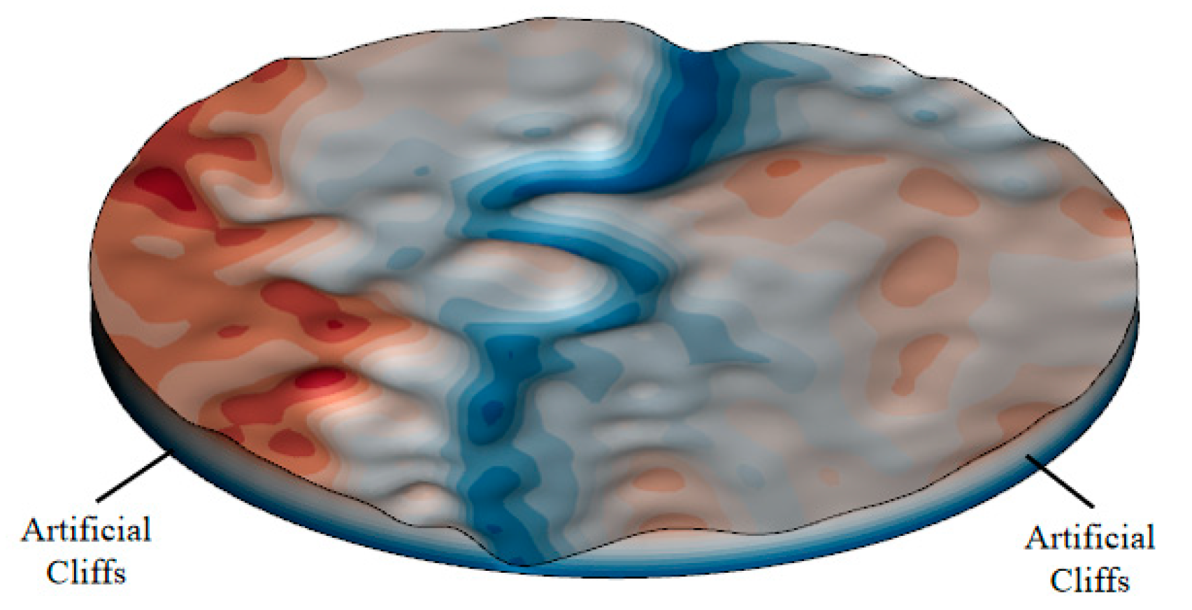
2.3. Optimization of Terrain Model BTS

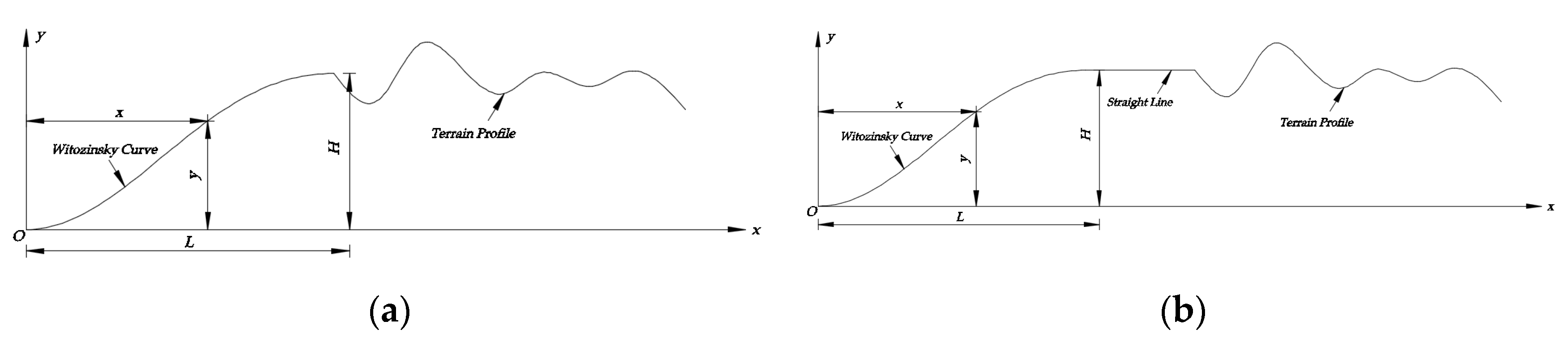
2.3.1. Form of Boundary Transition Section Curve

The Witozinsky curve was obtained in the case of an ideal axis of uncompressed axisymmetric flow. Wind tunnel operation results show that this kind of contraction curve can achieve good flow quality in test sections. Many low-speed wind tunnels constructed in 1960s by Chinese scholars were designed based on the Witozinsky formula (Wang et al. [43]). Evaluating the results of different contraction curves in terms of average wind speed reduction factors, vertical wind attack angles, and turbulence intensity, Huang et al. [44] drew a conclusion that the performance of the Witozinsky curve is the best and proposed an optimal curve expression of the Witozinsky curve at the same time. In his research, the terrain model boundary is directly connected to the BTS as shown in Figure 2a, which may lead to insufficient development of the inflow. In order to make the inflow develop fully, BTS in the present paper is improved by combining the Witozinsky curve with a horizontal line as shown in Figure 2b. The formula of the Witozinsky curve is shown as follows:

$$y=H\left\{1-\frac{{[1-{(x/L)}^2]}^2}{{[1+A{(x/L)}^2]}^3}\right\}$$

(6)

where $A=1/3$, H is the vertical distance from the highest point of the curve to the ground, $L$ is the horizontal projection length of the whole curve and the corresponding coordinates of any point on the curve is $(x,y)$.

2.3.2. Weight Allocation of Evaluation Indexes

Because the evaluation of BTS at the entrance of the terrain model mainly focuses on speed-up effect, the equivalent wind attack angle and the increase ratio of turbulence intensity, the specific evaluation indexes of effects of the terrain model BTS are defined as follows:

$$V_x={\displaystyle \sum _{k=1}^N\frac{v_k-v_{0k}}{v_{0k}}}\cdot \frac{\Delta h_k}{H_w}$$

(7)

$$A_x={\displaystyle \sum _{k=1}^N\frac{a_k\cdot \Delta h_k}{H_w}}$$

(8)

$$I_x={\displaystyle \sum _{k=1}^N\frac{I_k-I_{0k}}{I_{0k}}}\cdot \frac{\Delta h_k}{H_w}$$

(9)

where $N$ is the total amount of monitoring points. $v_k$ is the downward wind speed of the $k^{th}$ monitoring point from the ground and $v_{0k}$ is the wind speed at the $k^{th}$ monitoring point of the wind speed entrance. $\Delta h_k$ is the vertical distance between the $k^{th}$ monitoring point and the ${\left(k-1\right)}^{th}$ monitoring point. $H_w$ is the total height of the monitoring points. $a_k$ is the wind attack angle of the $k^{th}$ monitoring point from the ground. $I_k$ is the turbulence intensity at the $k^{th}$ monitoring point and $I_{0k}$ is the turbulent intensity at the $k^{th}$ monitoring point from the ground at the wind speed entrance.

The two-dimensional CFD simulation was used to optimize the parameters of the Witozinsky curve and horizontal line. For the indexes such as the speed-up ratio of wind speed, equivalent wind attack angle, and turbulence intensity increase ratio at the boundary of the terrain model, the weight allocation based on the correlation degree proposed by Tang (Tang et al. [45]) was adopted to determine the BTS curve parameters for a given total length of the transition section (Liu, et al. [32]).

There are $m=13$ schemes and $n=4$ indexes that have an influence on the comprehensive evaluation of each scheme. They can compose the matrix $X={(x_{ij})}_{m\times n}$. In this paper, the evaluation indexes are all cost indexes, which means that the smaller the index is, the better the result is. Standardize values in each column of $X={(x_{ij})}_{m\times n}$ using min-max standardization (shown in formula (10) to map each index of the matrix into [0,1]. After conversion, the dimensionless matrix is $X^{\prime }={(x_{ij})}_{m\times n}$. Then, select the maximum in each column of $X^{\prime }={(x_{ij})}_{8\times 6}$ to obtain the optimal objects $S_0^{+}$ and select the minimum in each column to get the worst object $S_0^{-}$. The correlation coefficient of each scheme with the optimal object and the worst object in each index can be calculated by Equations (11) and (12),

$$x^{\prime }=\frac{x-\min }{\max -\min }$$

(10)

$${\zeta }_{0^{+}i}(j)=\frac{1}{2{\Delta }_{0^{+}ij}+1}$$

(11)

$${\zeta }_{0^{-}i}(j)=\frac{1}{2{\Delta }_{0^{-}ij}+1}$$

(12)

where ${\Delta }_{0^{+}ij}=\left|x_{0^{+}j}-x_{ij}\right|$ and ${\Delta }_{0^{-}ij}=\left|x_{0^{-}j}-x_{ij}\right|$. The larger ${\zeta }_{0^{+}i}(j)$ is, the larger the correlation coefficient between scheme to be evaluated and the optimal scheme is in terms of index $j$. On the other hand, the performance of ${\zeta }_{0^{-}i}(j)$ is absolutely opposite.

Assume the weight vectors of $n$ indexes are $\omega =({\omega }_1,{\omega }_2,\dots \dots ,{\omega }_{n-1},{\omega }_n)$ respectively and $f(\omega )={\displaystyle \sum _{j=1}^n{\omega }_j^2}{[1-{\zeta }_{0^{+}i}(j)]}^2+{\displaystyle \sum _{j=1}^n{\omega }_j^2}{\zeta }_{0^{-}i}{(j)}^2$ represents the square sum of the weighted distance between the optimal solution and the worst one. Therefore, the smaller $f(\omega )$ is, the better scheme $i$ is. Establish the multi-objective programming model as follows:

$$\begin{array}{l}\min f(\omega )={(f_1(\omega ),f_2(\omega ),\dots \dots ,f_{m-1}(\omega ),f_m(\omega ))}^T\\ s.t.\{\begin{array}{l}{\displaystyle \sum _{i=1}^n{\omega }_j=1}\\ {\omega }_j\ge 0,j=1,2,\dots n-1,n\end{array}s.t.\{\begin{array}{l}\min {\displaystyle \sum _{i=1}^m{f}_i(\omega )}\\ {\displaystyle \sum _{i=1}^n{\omega }_j=1}\\ {\omega }_j\ge 0,j=1,2,\dots ,n-1,n\end{array}\end{array}$$

(13)

Since $f_i(\omega )\ge 0(i=1,2,\dots ,m-1,m)$, the multi-objective programming model is transformed into single-objective programming model. Establish Lagrange Function,

$$F(\omega ,\lambda )={\displaystyle \sum _{i=1}^m{\displaystyle \sum _{j=1}^n{\omega }_j^2\left\{{[1-{\zeta }_{0^{+}i}(j)]}^2+{\zeta }_{0^{-}i}{(j)}^2\right\}}}-\lambda ({\displaystyle \sum _{j=1}^n{\omega }_j-1})$$

(14)

$$\{\begin{array}{l}\frac{\partial F}{\partial {\omega }_j}=2{\omega }_j{\displaystyle \sum _{i=1}^m\left\{{[1-{\zeta }_{0^{+}i}(j)]}^2+{\zeta }_{0^{-}i}{(j)}^2\right\}}-\lambda =0\\ \frac{\partial F}{\partial \lambda }={\displaystyle \sum _{j=1}^n{\omega }_j-1=0}\end{array}$$

(15)

Solve Equation (15), the weight of $n$ indexes can be calculated by

$${\omega }_j=\frac{1}{u_j{\displaystyle \sum _{i=1}^n\frac{1}{u_j}}}$$

(16)

where $u_j$ is an intermediate variable and can be calculated by the following equation,

$$u_j={\displaystyle \sum _{i=1}^m\left\{{[1-{\zeta }_{0^{+}i}(j)]}^2+{\zeta }_{0^{-}i}^2(j)\right\}}$$

(17)

The final calculation results of all the wind profile positions are shown in

Table 1. Final results concerning weights at different wind profiles.

Horizontal Length (m)	Virtual Angle of BTS
	27°	30°	33°	36°	39°	42°	45°	48°	51°	54°	57°	60°	63°
0.0	1.06	0.89	1.46	1.51	1.56	1.62	1.98	1.7	1.75	1.79	1.89	1.98	2.17
0.2	0.88	0.92	0.96	0.99	1.01	1.05	1.74	1.1	1.12	1.15	1.22	1.3	1.51
0.4	0.6	0.64	0.66	0.68	0.7	0.73	1.14	0.76	0.78	0.8	0.83	0.88	1.03
0.6	0.36	0.38	0.4	0.41	0.43	0.45	0.7	0.46	0.47	0.49	0.51	0.53	0.6
0.8	0.2	0.22	0.23	0.24	0.25	0.26	0.44	0.27	0.28	0.29	0.3	0.31	0.34
1.0	−0.3	0.05	0.06	0.07	0.08	0.09	0.21	0.1	0.1	0.11	0.11	0.11	0.12

. The virtual angle is defined as the angle between the horizontal line and the line connecting the ground and the end of the Witozinsky curve. The horizontal length refers to the horizontal straight line length after the Witozinsky curve. Since the improved BTS proposed in this paper aims to provide an effective corrections for terrain models of wind tunnel test and CFD simulation, the total length of the improved BTS need to be sufficiently short to reduce blockage ratio while ensuring the accuracy of the wind characteristics over complex terrain; therefore, the total length of the improved BTS is regarded as the major consideration. If the total length of the horizontal projection is smaller than 1.0 m, the minimal final result is obtained at the combination of a virtual angle of 57° and a horizontal length of 0.8 m. Different optimal solutions can be obtained by changing the total horizontal projection length.

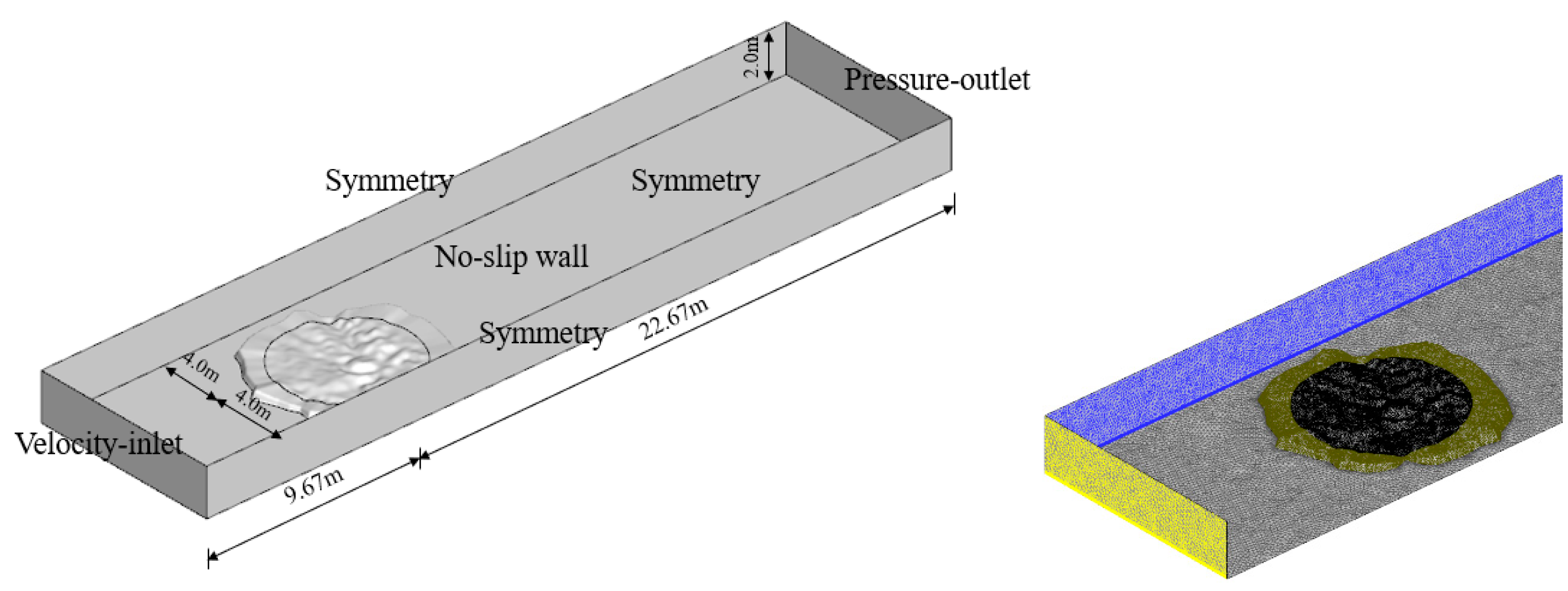
2.4. Numerical Terrain Model

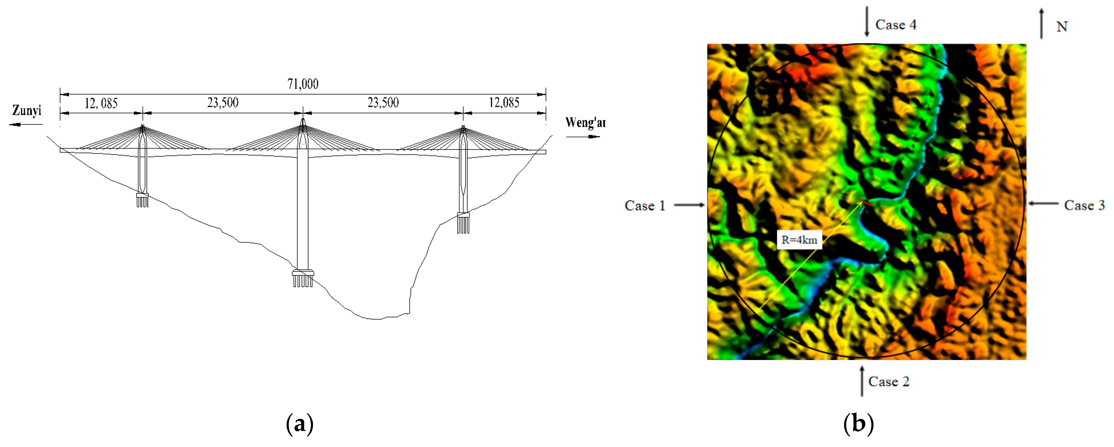
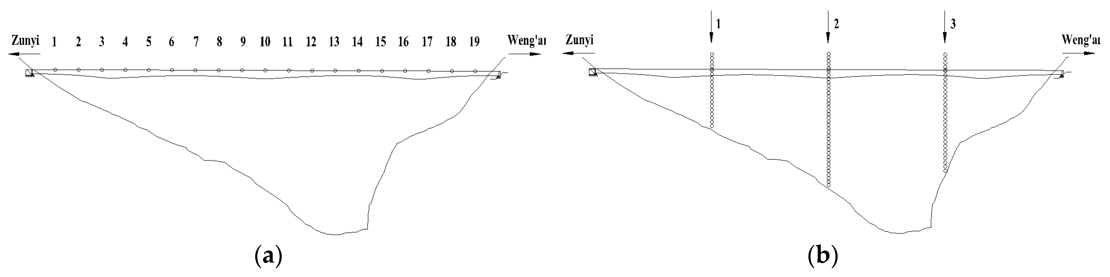
2.4.1. Survey of the Xiangjiang Bridge

The Xiangjiang Bridge is a four-span three-pylon cable-stayed bridge with span of 120 m + 235 m + 235 m + 120 m = 710 m. The main deck is 252.2 m above the bottom of the valley, as shown in Figure 3a. The balanced cantilever construction method are adopted to build the bridge, and the wind loads of the bridge with maximum double cantilever is the focus of wind-resistant design. Note that the bridge site is located in the mountainous terrain, as shown in Figure 3b. It can be seen from Figure 3b that the river approximately runs southwest to northeast, and the bridge is located in the center of the terrain. In order to determine the wind characteristics parameters for wind-resistant design of the bridge, numerical simulations and wind tunnel tests on wind characteristics over the mountainous terrain with/without BTS were carried out, respectively.

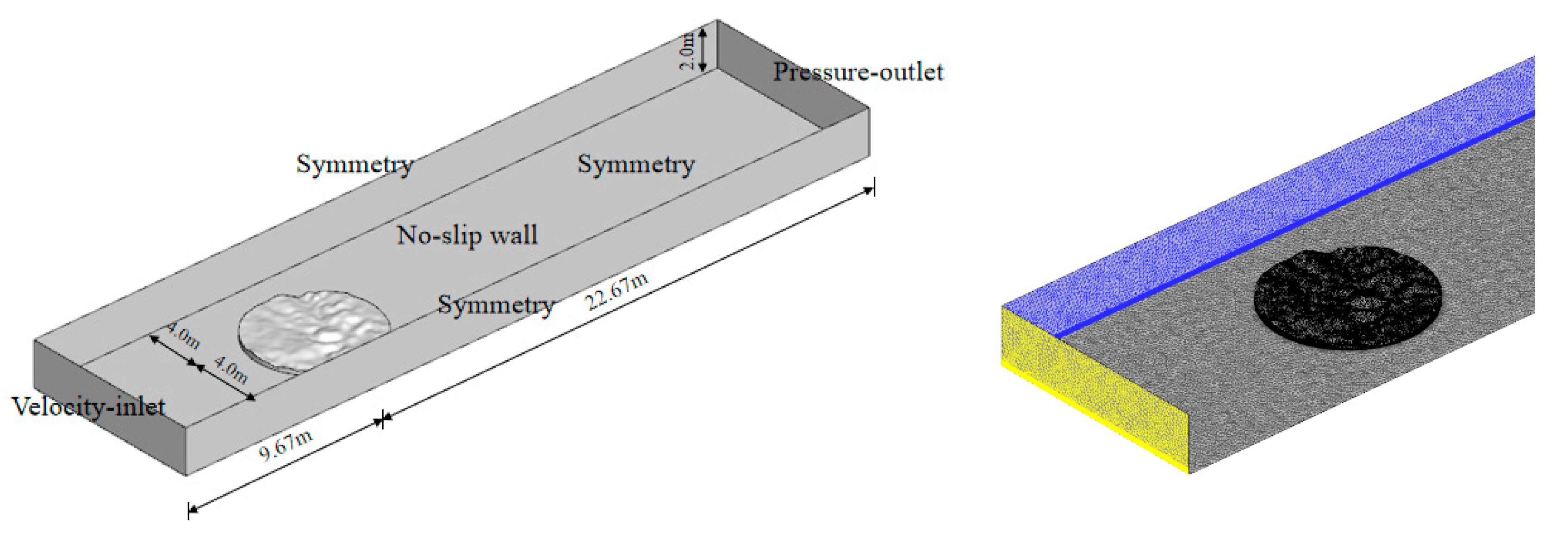
2.4.2. Terrain Model Construction

With reference to the existing literatures on mountainous terrain wind characteristics, as shown in

Table 2. Summary of main parameters of mountainous terrain models.

Number	Terrain Region	Geometry Scale Ratio	Methods and Domain	Authors
1	9.5 km × 7.3 km	-	CFD	Risan A., et al. [10]
2	D = 15 km	1:1000	Wind tunnel test: 36 m (L) × 22.5 m (B) × 4.5 m (H)	Li Y. et al. [29]
3	D = 12 km	1:1000	Wind tunnel test: 25 m(L) × 12.0 m(B) × 16.0 m (H)	Xu H. et al. [17]
4	D = 5.0 km	1:1500	Wind tunnel test	Pang J. et al. [27]
5	D = 9.0 km	1:1000	CFD: 15 m (L) × 15 m (B) × 4.5 m (H)	Hu P., et al. [31]
6	15 km × 14 km	-	CFD	Maurizi A., et al. [26]
7	D = 27.2 km	1:4000	Wind tunnel test: 14 m (L) × 15 m (B) ×2.0 m (H)	Chen F., et al. [23]

, the bridge site is taken as the center, and an area with a diameter of 8.0 km was selected to establish the mountainous terrain model. The computational domain with 32.34 m long, 8.0 m wide, 2.0 m high, and the geometry scale of 1:1500 were adopted according to the value of blockage ratio of the terrain model. The lowest elevation of the terrain model was taken as the bottom of the computational domain. The left side of the computational domain is defined as velocity-inlet boundary condition. The right side of the computational domain is defined as pressure-outlet boundary condition. The front, back, and top sides of the computational domain are defined as symmetry boundary conditions. The bottom of the computational domain is defined as non-slip wall boundary condition. The boundary conditions and computational domain of the terrain model without BTS are given in Figure 4. As can be seen in Figure 4, the distance between the center of the terrain model and the front and back walls of the computational domain is 4.0 m, respectively. The center of the terrain model is 9.67 m and 22.67 m away from the left and right sides of the computational domain.

The Power Law Profile Model is currently the only model of boundary layer wind profile [46]. The wind speed at the velocity inlet boundary after scaling of the computational domain are defined as follows:

$$\begin{array}{l}V(z)=V_{0.007}{\left(\frac{z}{0.007}\right)}^a,0\le z\le 0.233\mathrm{m}\\ V(z)=V_{ref},z>0.233\mathrm{m}\end{array}$$

(18)

where $z$ is the distance between the monitoring point and the ground; $a$ is the wind profile index and $a=0.16$ when the ground surface belongs to class-B wind field; $V(z)$ is the wind velocity of the monitoring point which is $z$ away from the ground; $V_{0.007}$ is the basic wind speed at the level of $z_0=0.007\mathrm{m}$ in the power law profile. $V_{ref}=V_{0.233}$ is the wind velocity when $z=0.233\mathrm{m}$.

In order to investigate the effects of the improved BTS on wind characteristics over mountainous terrain model, numerical simulation of the terrain model with/without BTS were conducted, respectively. With reference to the results of two-dimensional numerical simulation of the terrain model BTS, it is determined that the virtual inclination of the transition section is $\theta =57°$ and the length of the horizontal line is $L=0.80\mathrm{m}$ (Liu et al. [32]).

2.4.3. Grids of the Terrain Model

To ensure the numerical simulation accuracy of the terrain model grid, the grid independence checking was performed firstly. The mesh is divided into different parts. Unstructured prism was used to find grids near the ground, and the tetrahedral grid was adopted to reflect the undulating changes of the terrain. The near-wall grids of the terrain model are given in Figure 4. The detailed parameters of the three grids for independence checking are shown in

Table 3. Detailed setups of three grids of terrain model without BTS.

Grid	Mesh Size in Terrain Surface (m)	Mesh Size in Computation Domain (m)	Thickness of the First Boundary Layer Mesh (m)	Growth Rate of the Boundary Layer Mesh	Amount of Boundary Layer	Total Mesh Amount
G1	0.08	0.25	5	1.1	20	1,546,916
G2	0.07	0.20	5	1.1	20	3,881,449
G3	0.05	0.18	5	1.1	20	10,509,942

. The computational domain and grid arrangement of the terrain model with BTS are shown in Figure 5.

The flow solver used in this paper to simulate the wind characteristics over complex terrain is based on the finite-volume discretization in the space and the SIMPLEC (Semi implicit method for pressure linked equation consistent) pressure-correlation algorithm on a non-staggered grid arrangement (Kim, et al. [38]). The second-order cell-centered is adopted to deal with spatial discrete. The second-order upwind is used for time discrete. The time step is 0.015 s and the total amount of time steps is 10,000. According to the main parameters of wind-resistant design of the bridge, the mean cross-bridge wind speed and wind attack angles at the main deck level, longitudinal wind speed profiles at L/4, L/2 and 3L/4 of the bridge length were monitored to evaluate the calculation accuracy of different grids. The wind speed monitoring points are given in Figure 6.

The grid sensibility was conducted by taking case 1 without BTS as an example. Numerical results of mean cross-bridge wind speed and wind attack angles of grid G1, G2, and G3 at the main deck level over the terrain model without BTS are given in Figure 7a,b, respectively. The longitudinal wind speed profiles at L/4, L/2 and 3L/4 of the bridge length of grid G1, G2, and G3 over the terrain model without BTS are shown in Figure 7c. It can be found in Figure 7a that the mean cross-bridge wind speed of G2 agrees well with that of G3 with a relative error of 23% while the result of G1 departs from the results of the other two grid generations to a great extent with relative error 116%. Note that the same tendency can be found in Figure 7b (relative error 41% for terrain model with BTS while 160% without BTS) and (c), which means that relative sparse grid generation in the terrain model and computational domain will cause significant discrepancies in terms of average wind characteristics at bridge site. Therefore, the grid generation, G2, is considered to be the optimal grid since its amount of grids is less compared to G3 and the calculation accuracy can be guaranteed.

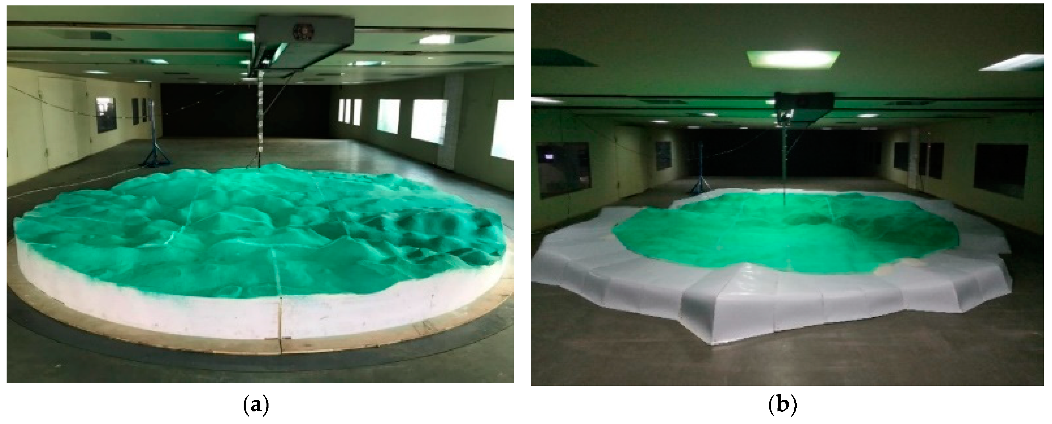
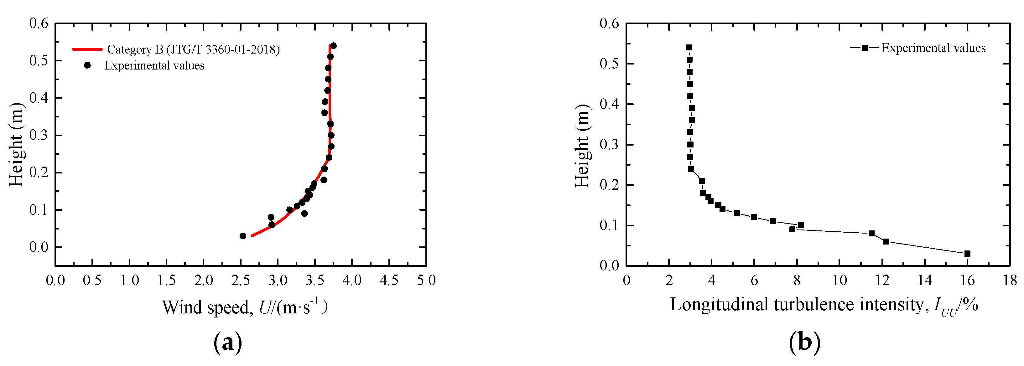
3. Wind Tunnel Test Set-Up

The wind tunnel tests were conducted in the third test section of HD-2 wind tunnel of Hunan University, Changsha, Hunan, China. HD-2 wind tunnel of Hunan University is 53 m long and 18 m wide, including three test sections. The first test section is 17 m long, 3 m wide, and 2.5 m high, and the wind speed of the test section was 0~58 m/s, which can be continuously adjusted. The second test section is 15 m long, 5.5 m wide and 4.4 m high, and the maximum wind speed was 18 m/s. The third test section was 15 m long, 8.5 m wide and 2 m high, and the maximum wind speed was 15 m/s. Considering the size of the third section of HD-2 wind tunnel, the terrain model centered on the mid-span of the bridge with a geometric scale of 1:1500 was designed and fabricated to simulate a region with a diameter of 8 km. The average height of the terrain model was roughly 0.2 m. The blockage ratio is defined as the ratio of cross-sectional area of the terrain model and the wind tunnel test section. If the blockage ratio of the terrain model is too large, the inflow cannot develop fully, leading to inaccurate prediction of the wind field over complex terrain. The blockage ratio of the terrain model is about 6.27%, which is within the range of 5.0% and 10% required in Design Rules for Aerodynamic Effects on Bridges published by British.

To investigate the BTS effects on wind characteristics over mountainous terrain model, the wind tunnel tests of terrain model with/without BTS were conducted, respectively. The geometric parameters of the BTS are consistent with these of the CFD simulation model. Figure 8 shows the terrain model with/without BTS.

Before the wind tunnel test of terrain model was carried out, the inflow wind speed and turbulence intensity profiles in the empty wind tunnel section was conducted first. The total height of the monitoring points was 0.6 m, and the interval between two adjacent monitoring points was 0.03 m. The first monitoring point was 0.03 m away from the bottom of the wind tunnel section. The wind speed was measured by Cobra probes from TFI (Turbulent Flow Instrumentation Pty Ltd., Victoria, Australia). Figure 9 shows the comparison of the wind profile of the incoming wind speed in the empty wind tunnel section and the wind profile of terrain category B suggested in wind-resistant design specification for highway bridges (JTG/T 3360-01-2018). As shown in Figure 9a, the measured inflow wind speed profile in the empty wind tunnel section was closed to the corresponding wind speed profile of category B. The main reason is that the geometric scale of the terrain model is 1:1500, the height of the boundary layer of the terrain category B was 0.233 m, which was approximately close to the boundary layer height in the wind tunnel test section under a uniform inflow condition. It can be seen from Figure 9b that the longitudinal turbulence intensity was about 3.0% when the height of the monitoring points is larger than 0.2 m.

To find out the influence of wind yaw angles on wind characteristics over mountainous terrain, four cases of wind from the west, south, east, and north were investigated by numerical simulations and wind tunnel tests, respectively. The wind yaw angle was 0° when the inflow enters the terrain model along the west. Counterclockwise rotation was positive for the wind yaw angle and the detailed test cases are shown in Figure 3b.

4. Verification of Improved BTS

Due to space limitations, only wind speed, turbulence kinetic energy, and wind attack angle of case 1 as well as 2, without and with improved BTS are compared to verify its effect.

It can be seen from Figure 10 that when there is improved BTS, wind speed distribution is more uniform and closer to that of the inflow wind speed profile. Besides, there is no flow separation near the boundary of the terrain model.

Turbulence kinetic energy (TKE) is a measure of the intensity of turbulence and determines the ability of the flow to maintain turbulence or become turbulence, thus indicating flow stability. From Figure 11, it can be concluded that at the inlet of the terrain model without improved BTS, the TKE with BTS is smaller than that of the terrain model without BTS, which indicates that the improved BTS is able to reduce turbulence intensity induced by artificial cliffs and uplift the inflow gradually.

Wind attack angles induced by artificial cliffs will have a significant influence on the wind attack angle at the bridge site, thus reducing wind attack angles at the inlet boundary hold a decisive place in wind characteristic prediction over complex terrain. As shown in Figure 12, the wind attack angle at the inlet boundary with the improved BTS is much smaller than that without BTS and is closer to zero, indicating that the improved BTS can reduce the wind attack angle caused by artificial cliffs to a great extent.

In conclusion, by comparing wind speed, turbulence kinetic energy, and wind attack angle near the inlet of the terrain model without and with improved BTS, the BTS can effectively reduce the impact of artificial cliffs on wind characteristics after the inlet boundary.

5. Numerical and Experimental Results

According to the wind-resistance design requirements of the bridge, the cross-bridge wind speed, wind attack angles at main deck level, and longitudinal wind speed profiles at L/4, L/2, and 3L/4 of the bridge length were analyzed for numerical and experimental cases. In this paper, the positive direction of cross-bridge wind is from southwest to northeast, and the positive of attack angle is from underside to upside of the main deck. Here, cross-bridge wind speeds are all normalized by the horizontal component of the gradient wind speed of inflow wind, namely

$${\overline{V}}_H=\frac{V_H}{V_{ref}\cdot \cos \beta }$$

(19)

where ${\overline{V}}_H$ is the non-dimensional cross-bridge wind speed, $V_H$ is the cross-bridge wind speed, $V_{ref}$ is the gradient wind speed of inflow above which the wind speed remains unchanged with the increase of altitude, $V_{ref}=3.70\mathrm{m}/\mathrm{s}$, and $\beta$ is the angle between inflow wind direction and perpendicular of the bridge axis.

Wind attack angle at the main deck level is defined as follows:

$$\alpha =\arctan \left(\frac{V_V}{V_H}\right)$$

(20)

where $\alpha$ is the wind attack angle at main deck level, $V_V$ is the vertical wind speed at main deck level, and $V_H$ is the cross-bridge wind speed at main deck level.

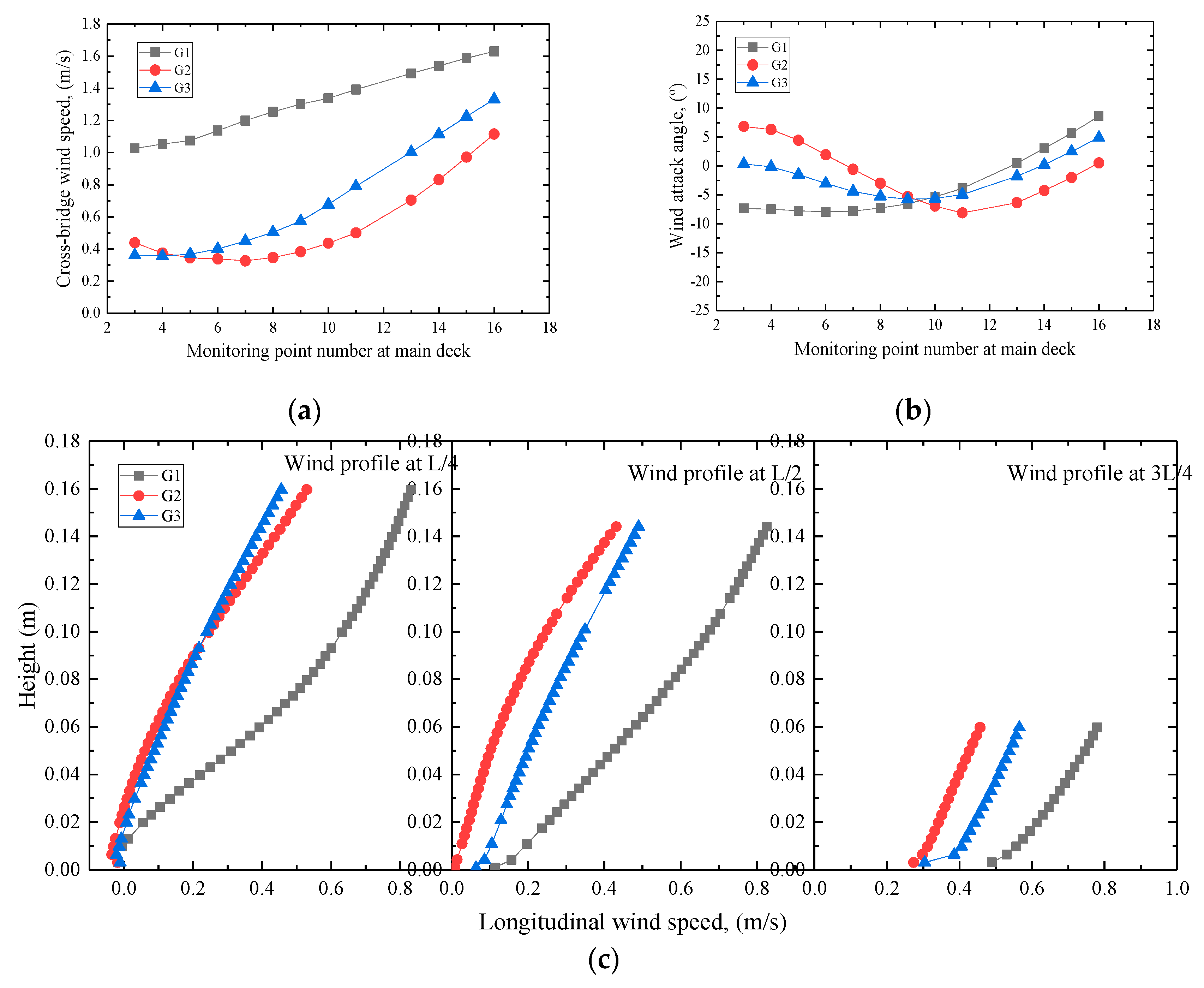
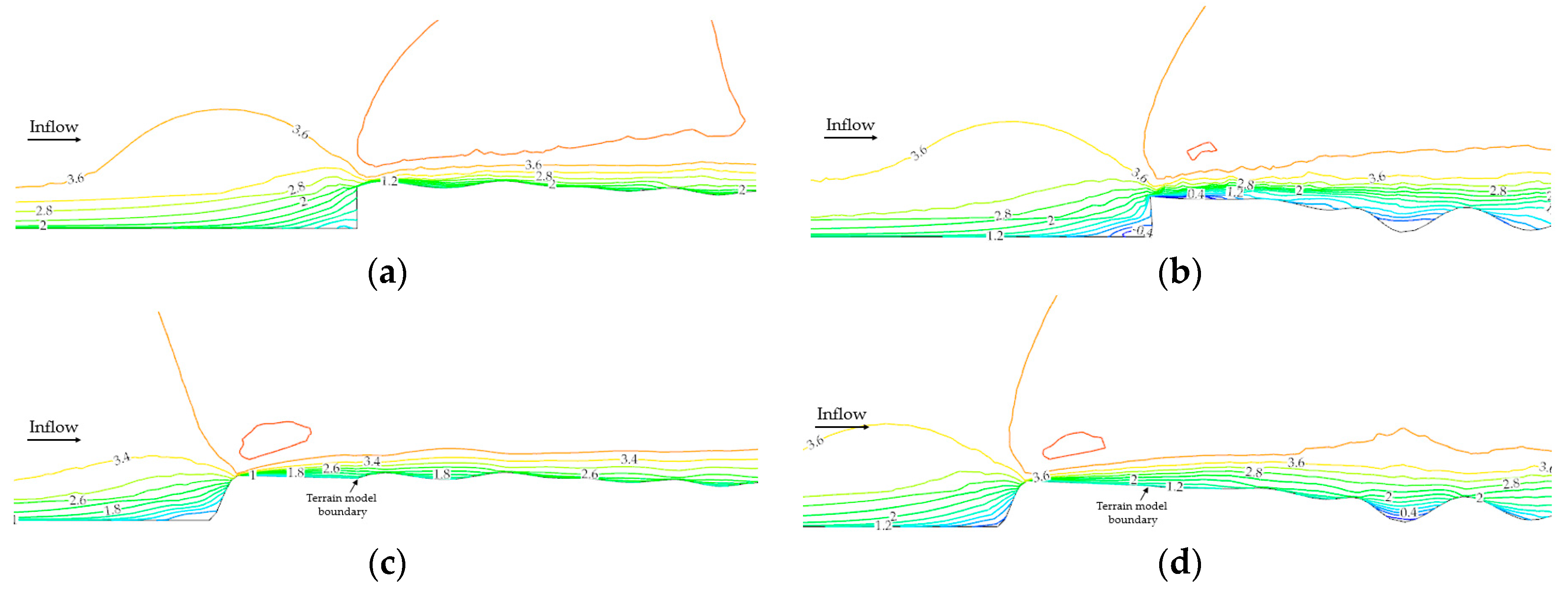
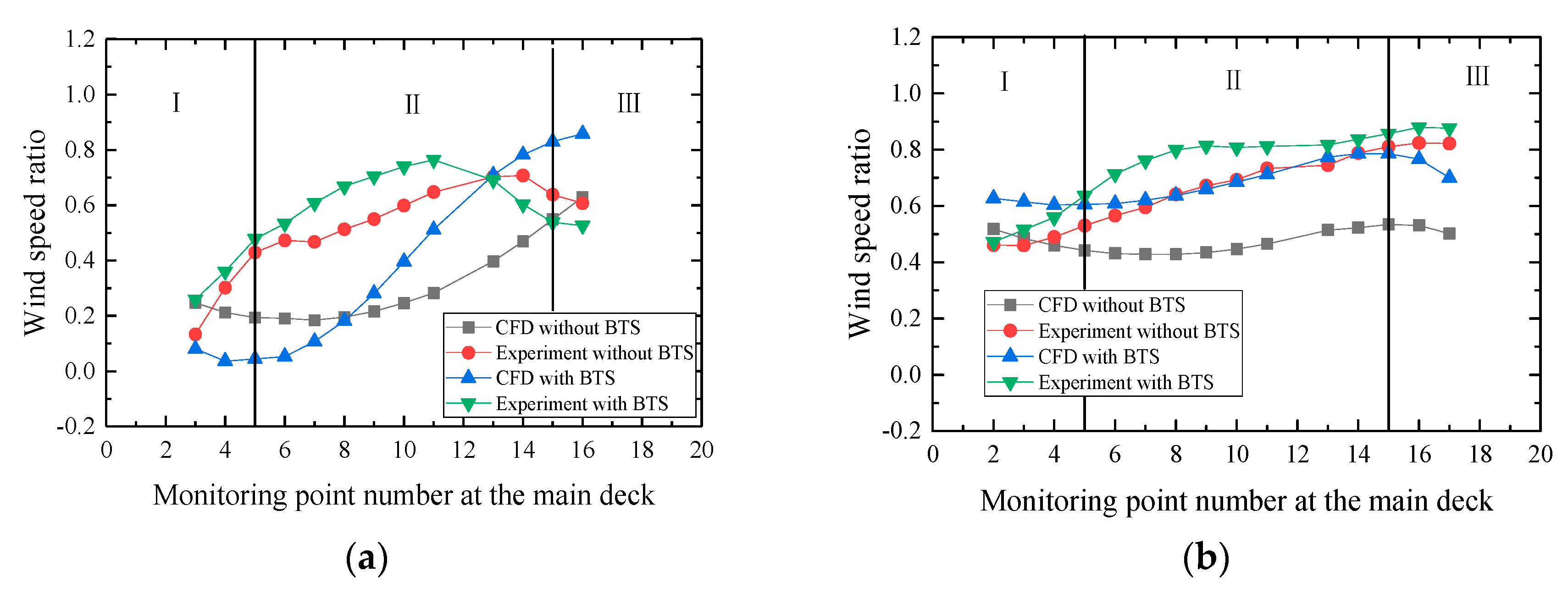
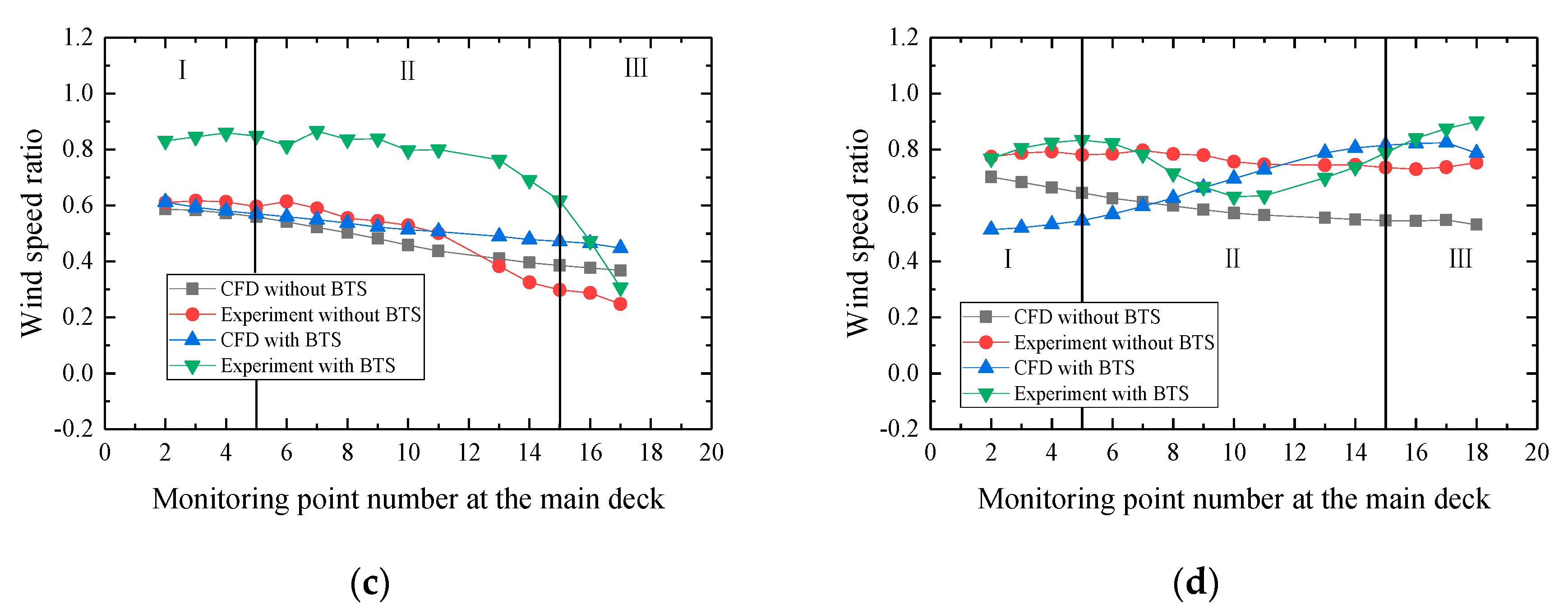
5.1. Cross-Bridge Wind Speed at Main Deck Level

The numerical and experimental results of the non-dimensional cross-bridge wind speed at main deck level under different cases are given in Figure 13. Considering the span layout characteristics large-span bridges, it can be roughly divided into three parts along bridge axis; namely, mountain areas (I, III) and the central canyon area (II).

From Figure 13a, it can be seen that for case 1 (wind blows from the west), the non-dimensional cross-bridge wind speed at the main deck level varies greatly along the bridge axis. The non-dimensional cross-bridge wind speed in part III was relatively large, while that in part I was relative small. For experimental results, the cross-bridge wind speed of the terrain model with BTS was generally larger than that of the terrain model without BTS. For case 1, due to the topographic effects, there was a certain deviation between the numerical simulation results of the cross-bridge wind speed at the main deck level and the experimental results.

From Figure 13b, it can be seen that for case 2 (wind blows from the south), the non-dimensional cross-bridge wind speed at the main deck level varies along the bridge axis. The non-dimensional cross-bridge wind speed in part III is relatively large, while the cross-bridge wind speed in part I was relative small. For experimental results, the cross-bridge wind speed of the terrain model with BTS was generally larger than that of the terrain model without BTS. The numerical simulation results also show the same trend.

From Figure 13c, it can be seen that for case 3 (wind blows from the east), the non-dimensional cross-bridge wind speed at the main deck level varies little along the bridge axis. The non-dimensional cross-bridge wind speed in part III was relatively large, while the non-dimensional cross-bridge wind speed in part I is relatively small. For both the experimental results and numerical results, the cross-bridge wind speed of the terrain model with BTS was generally larger than that of the terrain model without BTS. Besides, it can be seen from Figure 13c that little difference of the wind characteristics with and without improved BTS was found, which indicated that the effect of improved BTS depends on the inflow direction. The altitude in the east over the complex terrain was high. When the height difference between the inlet boundary and the bridge site is large, the flow separation is severe and the effect of the improved BTS on flow separation is limited. Thus, the relation between the height difference and the improved BTS can be evaluated in future research.

From Figure 13d, it can be seen that for case 4 (wind blows from the north), the non-dimensional cross-bridge wind speed at the main deck level varies little along the bridge axis. For experimental results, the cross-bridge wind speed of the terrain model with BTS is generally smaller than that of the terrain model without BTS in part II. For numerical simulation results, the cross-bridge wind speed of the terrain model with BTS was generally larger than that of the terrain model without BTS in part II.

In conclusion, in cases 1 to 3, the wind tunnel test results of the terrain model show that the cross-bridge wind speed ratio at the main deck level of the terrain model with the improved BTS was relatively larger than that of the terrain model without BTS. A similar tendency can be found from numerical results of the terrain model with/without BTS. Thus, if the there is no improved BTS in front of the terrain model, the cross-bridge design wind speed of the bridge deck may be underestimated. It is recommended to use the improved BTS for terrain model boundary correction.

The statistical values of numerical results and experimental results of non-dimensional cross-bridge wind speed at main deck level under different cases are shown in Figure 14. It can be seen from Figure 14 that though there are some discrepancies between the wind tunnel tests results and numerical simulation results, the majority of the data is located within relative errors of 30%. This kind of error is indeed unavoidable because the scale of terrain model was small which made it a challenge to place the model in the exact center of the test section and find the accurate monitoring point positions as CFD simulation did. Thus, the wind tunnel test results can be regarded as accurate ones, and the results from CFD simulations can be used for qualitative analysis.

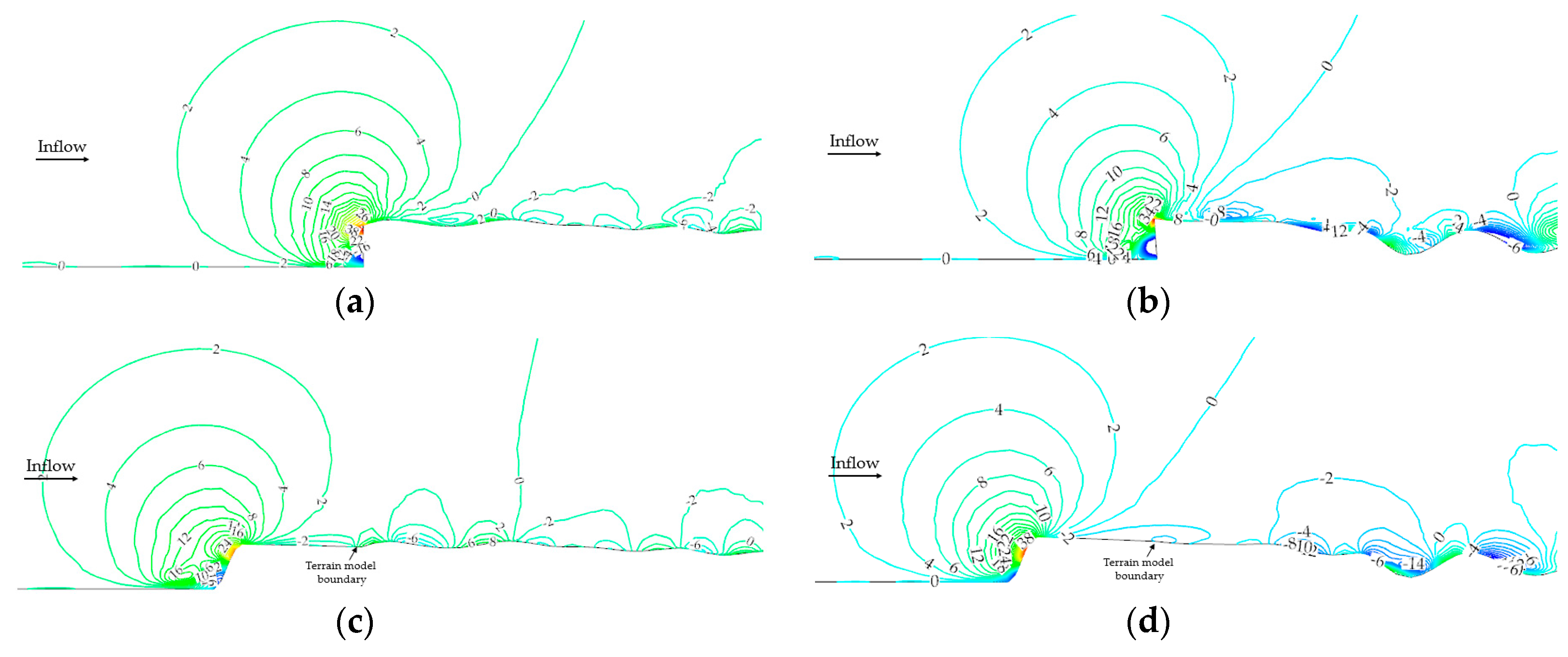
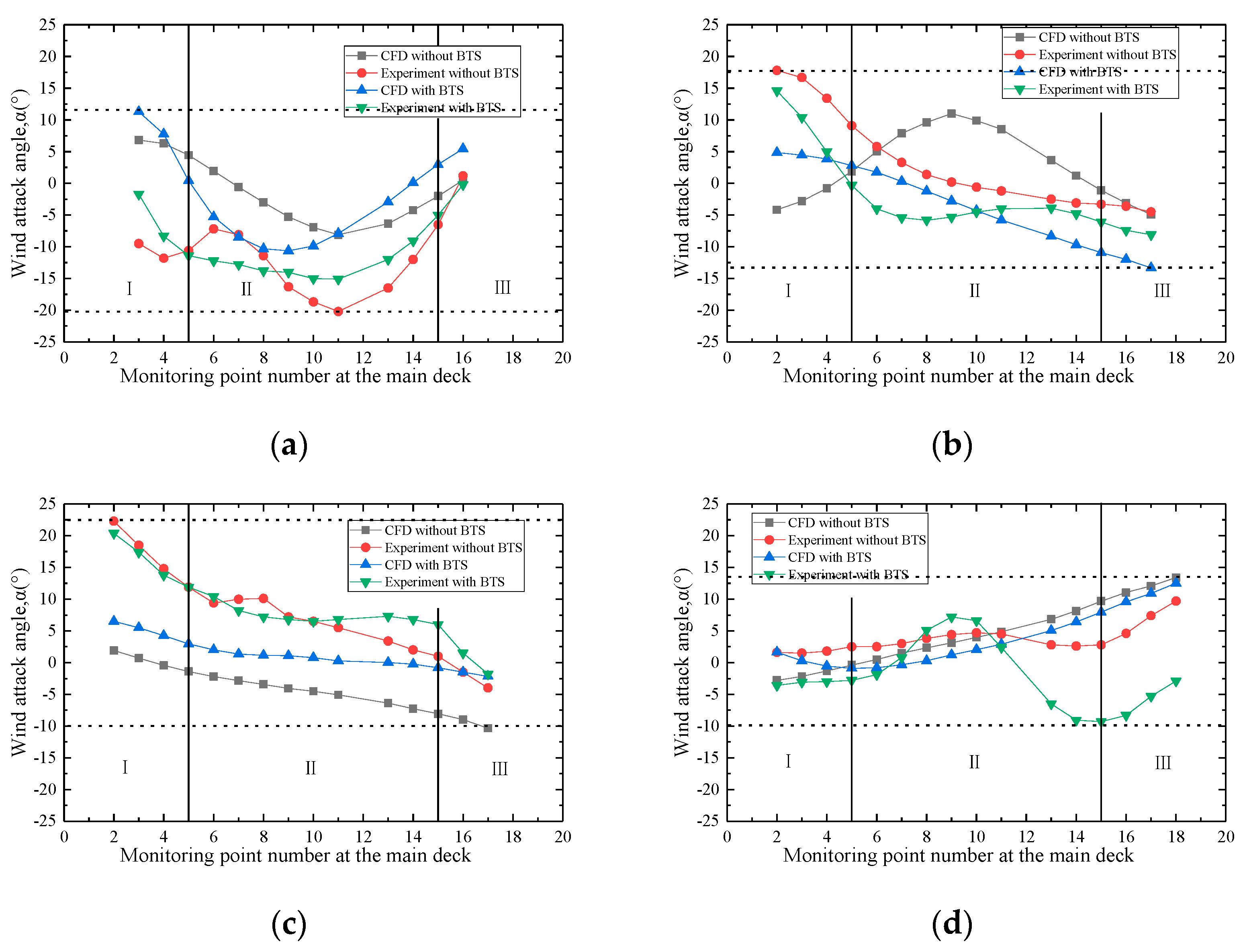
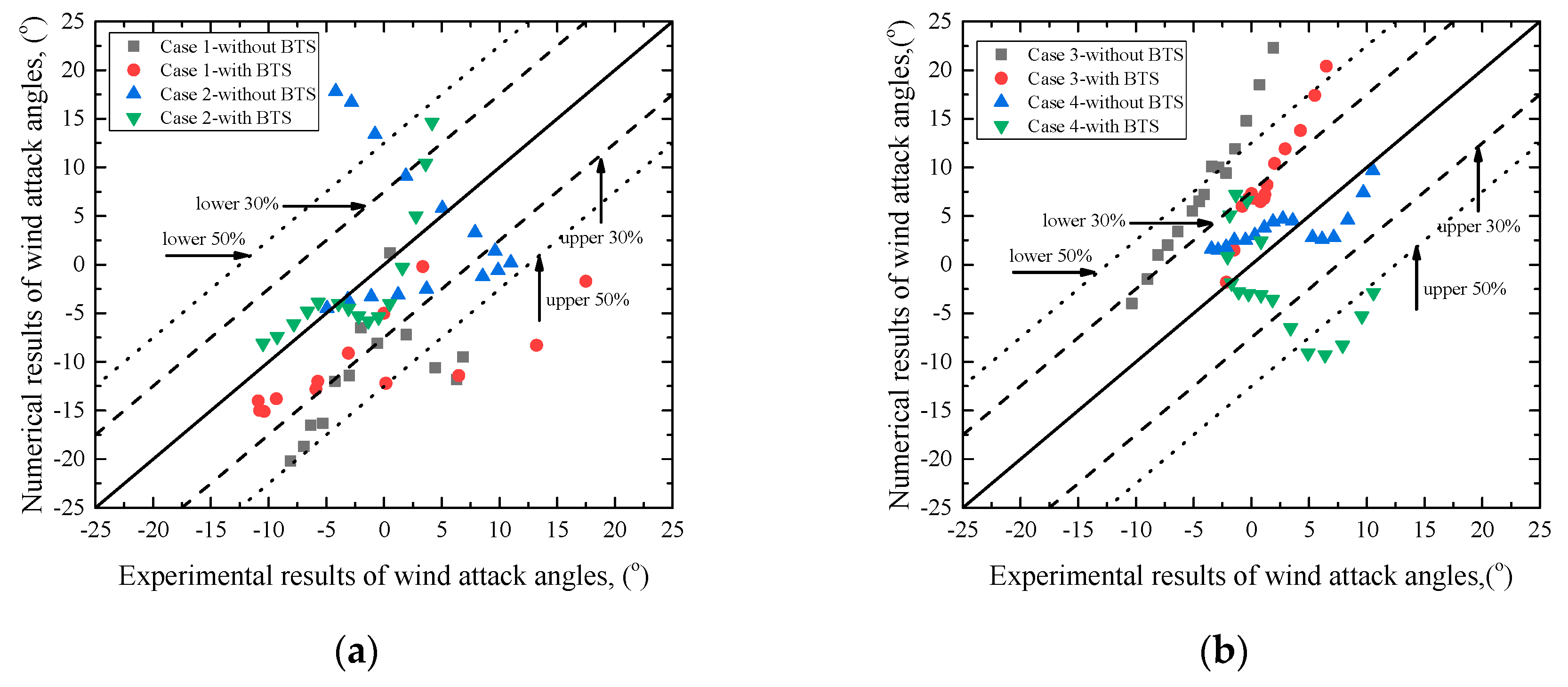
5.2. Wind Attack Angles at Main Deck Level

The numerical and experimental results of the wind attack angle at main deck level of the bridge for different cases are given in Figure 15. From Figure 15a, it can be seen that for case 1 (wind blows from the west), the wind attack angle at the main deck level of the bridge varied greatly along the bridge axis, which can be roughly divided into three parts; namely, mountain areas (I, III) and the central canyon area (II). For experimental results, the wind attack angles at the main deck level of the terrain model with BTS is about −15°~−10° in part II, while the wind attack angles at the main deck level of the terrain model without BTS is −20°~−5° in part II. For numerical results, the wind attack angles at the main deck level of the terrain model with BTS was about −10°~0°, while the wind attack angles at the main deck level of the terrain model without BTS was −7.5°~5°.

From Figure 15b, it can be seen that for case 2 (wind blows from the south), the wind attack angle at the main deck level of the bridge changes along the bridge axis. For experimental results, the wind attack angles at the main deck level of the terrain model with BTS was about −5°~0° in part II, while the wind attack angles at the main deck level of the terrain model without BTS was −5°~10° in part II. For numerical results, the wind attack angles at the main deck level of the terrain model with BTS was about −12°~2°, while the wind attack angles at the main deck level of the terrain model without BTS was about 0°~10°.

From Figure 15c, it can be seen that for case 3 (wind blows from the east), for experimental results, the wind attack angles at the main deck level of the terrain model with BTS were about 5°~12°in part II, while the wind attack angles at the main deck level of the terrain model without BTS were 1°~12° in part II. For numerical results, the wind attack angles at the main deck level of the terrain model with BTS are about 0°~3°, while the wind attack angles at the main deck level of the terrain model without BTS were about −7°~−2°.

From Figure 15d, it can be seen that for case 4 (wind blows from the north), the experimental results of the wind attack angles at the main deck level of the terrain model with BTS were about −10°~7°, while the wind attack angles at the main deck level of the terrain model without BTS were about 3°~ 5°. For numerical simulation results, the wind attack angles at the main deck level of the terrain model with BTS were about −0.5°~7.5°, while the wind attack angles at the main deck level of the terrain model without BTS were about −0.5°~10°.

In general, both numerical simulation and experimental results under different cases show that the range of the wind attack angles at the main deck level in part II with BTS is smaller than that of the terrain model without BTS. The reason is that the existence of the BTS effectively reduces the influence of artificial cliffs. Thus, the turbulence development of wind field with BTS is more sufficient than that without BTS; the wind attack angles with BTS are smaller than that without BTS.

The statistical values of numerical and experimental results of the wind attack angles at main deck level under different cases are shown in Figure 16. It can be seen from the Figure 16 that though there are some discrepancies between the wind tunnel tests and numerical simulation, the majority of the deviation is located within relative errors of 30%.

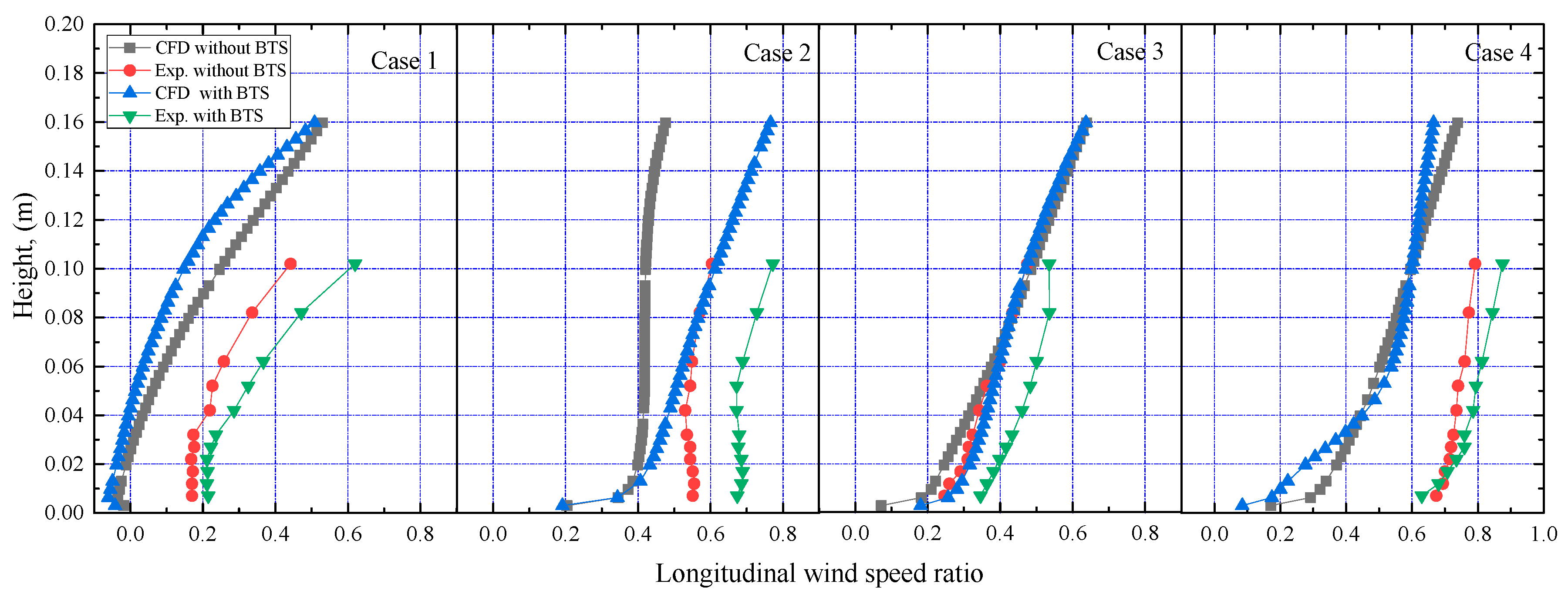
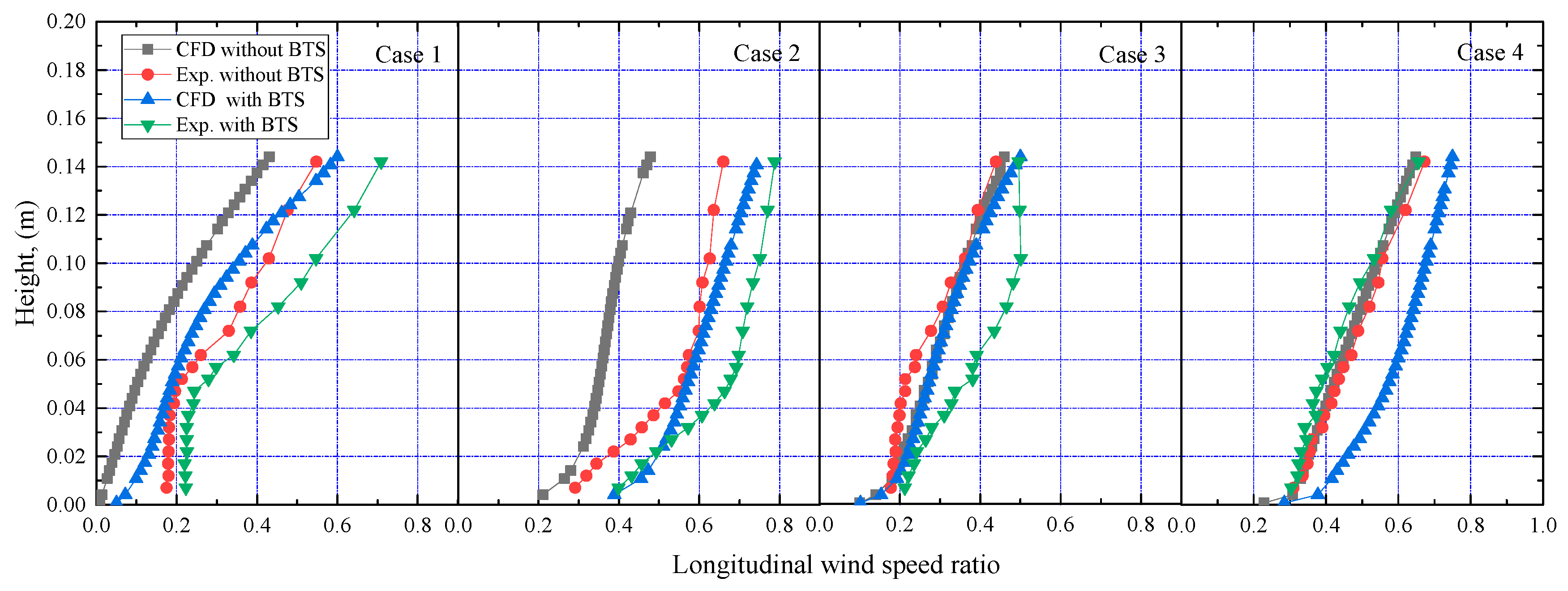
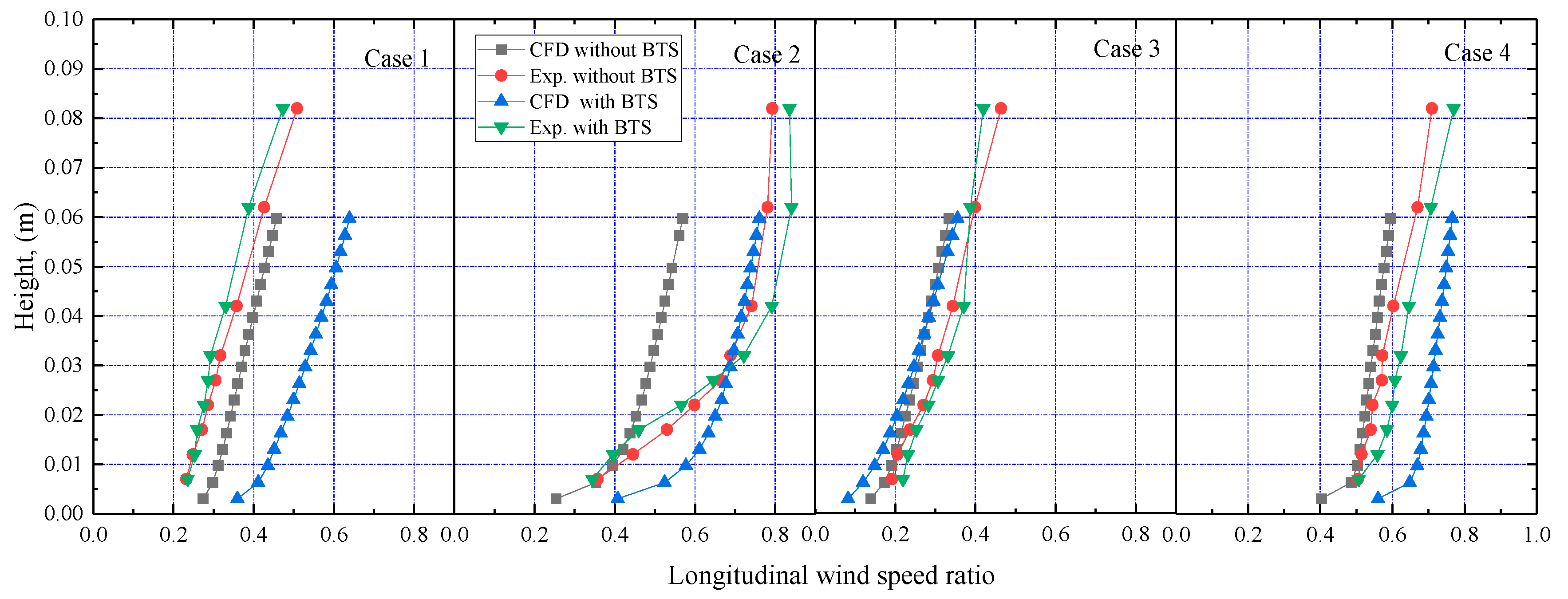
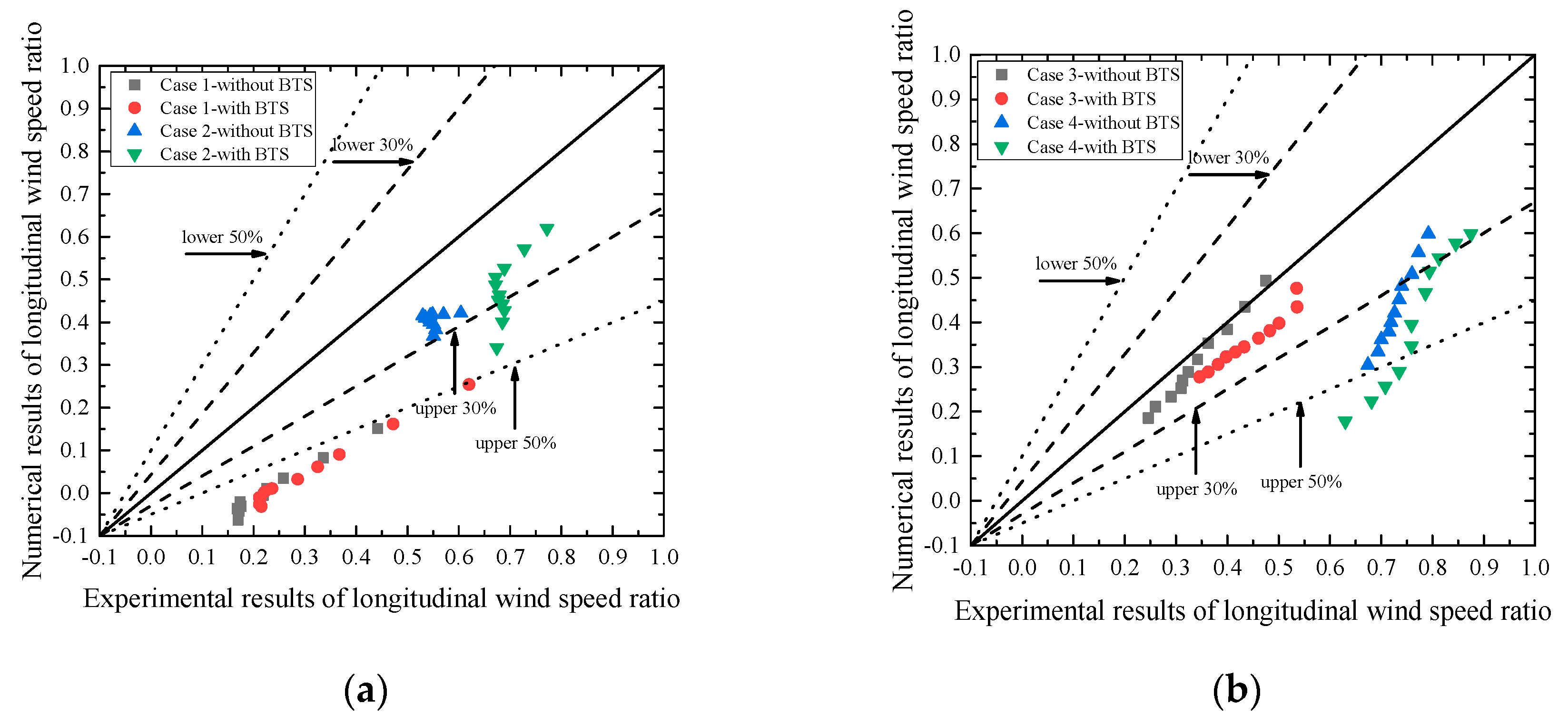
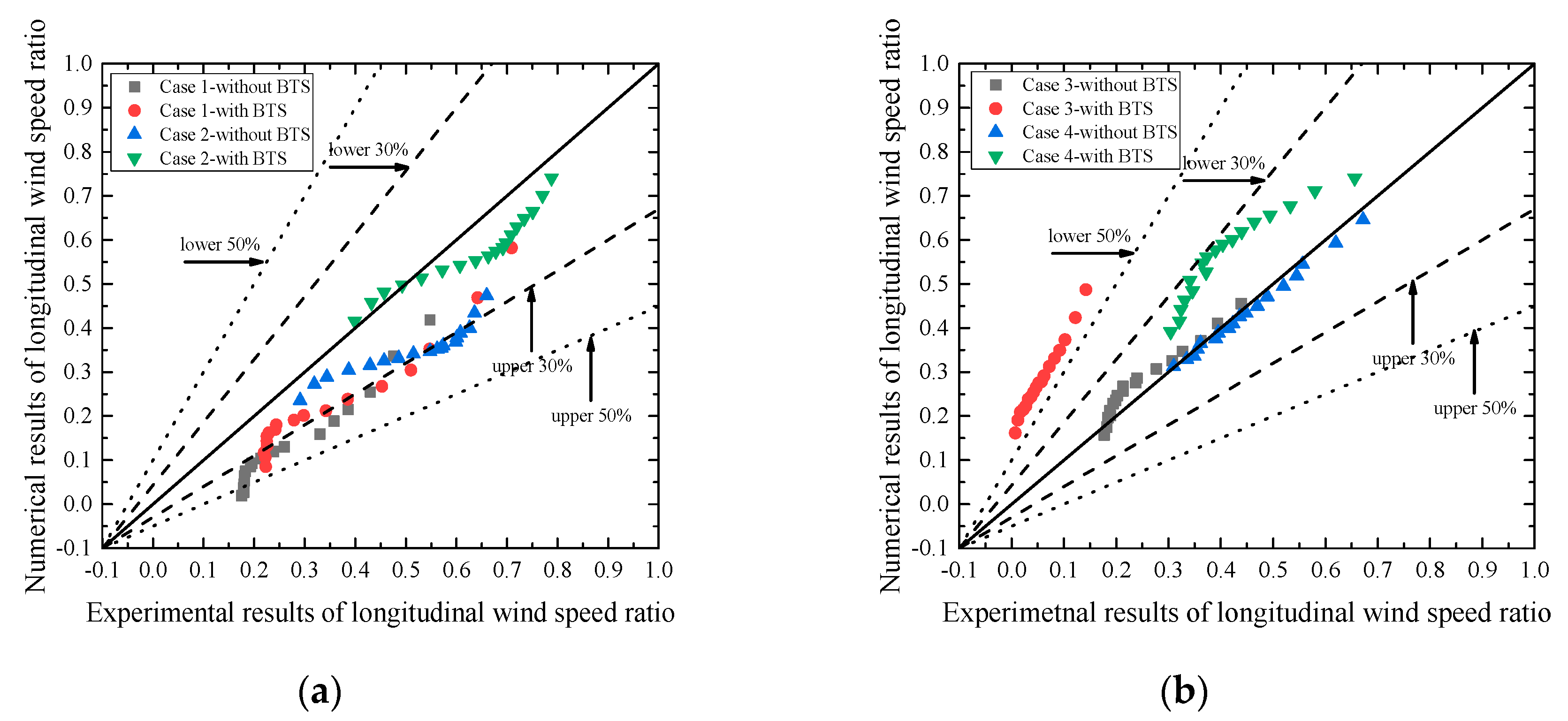
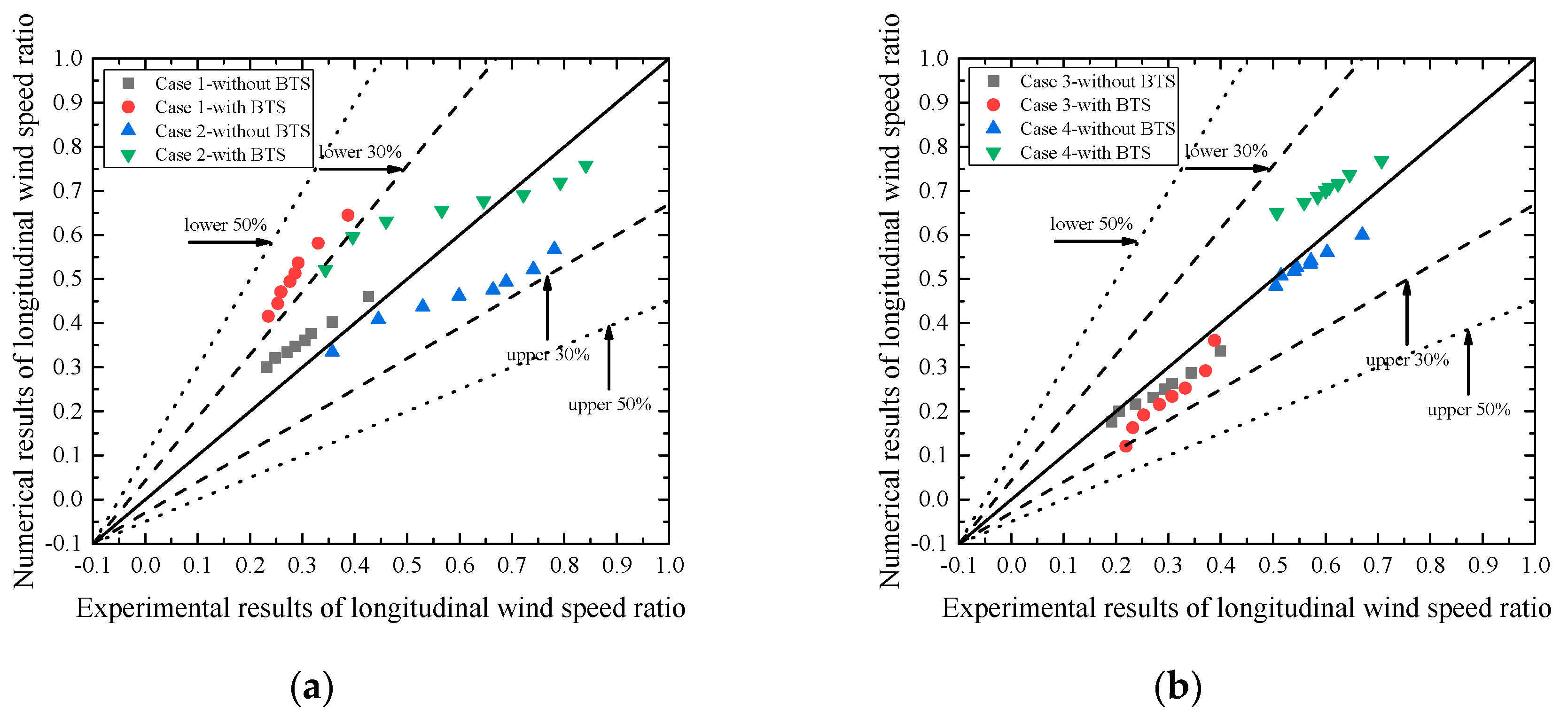
5.3. Wind Profiles at L/4, L/2 and 3L/4 of Bridge Length

The longitudinal wind speed ratio is defined as the measured longitudinal wind speed above the terrain model divided by longitudinal wind speed of the corresponding inflow boundary layer. The numerical and experimental results of longitudinal wind speed ratio profiles at L/4, L/2 and 3L/4 of the bridge length are given in Figure 17, Figure 18 and Figure 19. As shown in Figure 17, Figure 18 and Figure 19, the longitudinal wind speed ratio at different positions, namely L/4, L/2 and 3L/4 of the bridge length, generally increase with height.

As shown in Figure 17, the experimental results of longitudinal wind speed ratio were larger than the numerical results at L/4 of bridge length for case 1 (wind blows from the west) and case 4 (wind blows from the north), respectively. The experimental results of longitudinal wind speed ratio were slightly larger than the numerical results at L/4 of bridge length for case 2 (wind blows from the south) and case 3 (wind blows from the east), respectively. The experimental results of the longitudinal wind speed ratio at L/4 of the bridge length shows that the longitudinal wind speed ratio of terrain model with BTS were larger than that of the terrain model without BTS for different cases. The numerical results at L/4 of the bridge length shows that the longitudinal wind speed ratio of terrain model with BTS were slightly larger than that of terrain model without BTS under cases 2 to 4, except for case 1.

As shown in Figure 15, the experimental results of longitudinal wind speed ratio at L/2 of bridge length were larger than the numerical results for case 1 (wind blows from the west) and case 2 (wind blows from the north), respectively. The experimental results of longitudinal wind speed ratio were close to the numerical results for case 3 (wind blows from the east) and case 4 (wind blows from the north), respectively. The experimental results of the longitudinal wind speed ratio at L/2 of the bridge length shows that the longitudinal wind speed ratio of terrain model with BTS were larger than that of the terrain model without BTS for cases 1 to 3, except for case 4. The numerical results of the longitudinal wind speed ratio at L/2 of the bridge length shows that the longitudinal wind speed ratio of terrain model with BTS were slightly larger than that of terrain model without BTS under cases 1, 2, and 4, except for case 3.

As shown in Figure 16, the experimental results of longitudinal wind speed ratio at 3L/4 of bridge length are close to the numerical results for cases 2 to 4. The experimental results of longitudinal wind speed ratio at 3L/4 of bridge length were smaller than the numerical results for case 1. The experimental results shows that the longitudinal wind speed ratio of terrain model with BTS were slightly smaller than that of the terrain model without BTS for case 1 while the longitudinal wind speed ratios of the terrain model with BTS were slightly larger than that of the terrain model without BTS for cases 2 to 4.

The statistical values of the numerical and experimental results of longitudinal wind speed ratio at L/4, L/2 and 3L/4 under different cases are given in Figure 20, Figure 21 and Figure 22. From Figure 20a, it can be seen that the relative error between numerical and experimental results of longitudinal wind speed ratios at L/4 of the bridge length under case 1 with/without BTS were about 50%, while the relative error between numerical and experimental results of longitudinal wind speed ratios at L/4 of the bridge length under case 2 with/without BTS were about 30%. From Figure 20b, it can be seen that the relative error between numerical and experimental results of longitudinal wind speed ratio at L/4 of the bridge length under case 3 and 4 with/without BTS were about 30%. As shown in Figure 18, the relative error between numerical and experimental results of longitudinal wind speed ratios at L/2 of the bridge length under different cases with/without BTS were less about 30% except for case 3 with BTS. From Figure 22, the relative error between numerical and experimental results of longitudinal wind speed ratios at 3L/4 of the bridge length under different cases with/without BTS were less than 30%. In general, it can be seen from the Figure 20, Figure 21 and Figure 22 that though there were some discrepancies between the wind tunnel tests and numerical simulation, the majority of the data are located within relative errors of 30%.

6. Conclusions

To study the wind characteristics over mountainous terrain, the Xiangjiang Bridge site was employed in this paper. The improved boundary transition sections were adopted to reduce the influence of the artificial cliffs on the edge of the terrain model on the wind characteristics at the bridge site over the mountainous terrain. The mean cross-bridge wind speed and wind attack angles at the main deck level, longitudinal wind speed profiles at L/4, L/2, and 3L/4 of the bridge length were investigated in detail with the assistance of numerical simulations and wind tunnel tests. The main conclusions are summarized as follows:

• The cross-bridge wind speeds and wind attack angles at the main deck level of the bridge at mountainous terrain site vary greatly along the bridge axis. Considering the span layout characteristics large-span bridges, it can be roughly divided into three parts along bridge axis, namely, mountain areas (I, III) and central canyon area (II). The changes in wind characteristics near the mountain areas (I, III) were relatively large, while the changes in wind speed and wind attack angles in the central canyon area (III) were relatively small.
• Experimental and numerical results show that the cross-bridge wind speed at the main deck level of the mountainous terrain model with BTS was generally larger than that of the mountainous terrain model without BTS in the central canyon area (II) for most cases, which needs to be paid special attention in wind-resistance design of the bridge. If there is no improved BTS in front of the terrain model, the cross-bridge design wind speed of the bridge deck may be underestimated.
• In general, the range of wind attack angles at the main deck level of the mountainous terrain model with BTS within 1/4 to 3/4 of the bridge length; namely, in the central canyon area (II), are smaller than the range of wind attack angles of the mountainous terrain model without BTS. It is recommended to use the improved BTS for terrain model boundary correction.
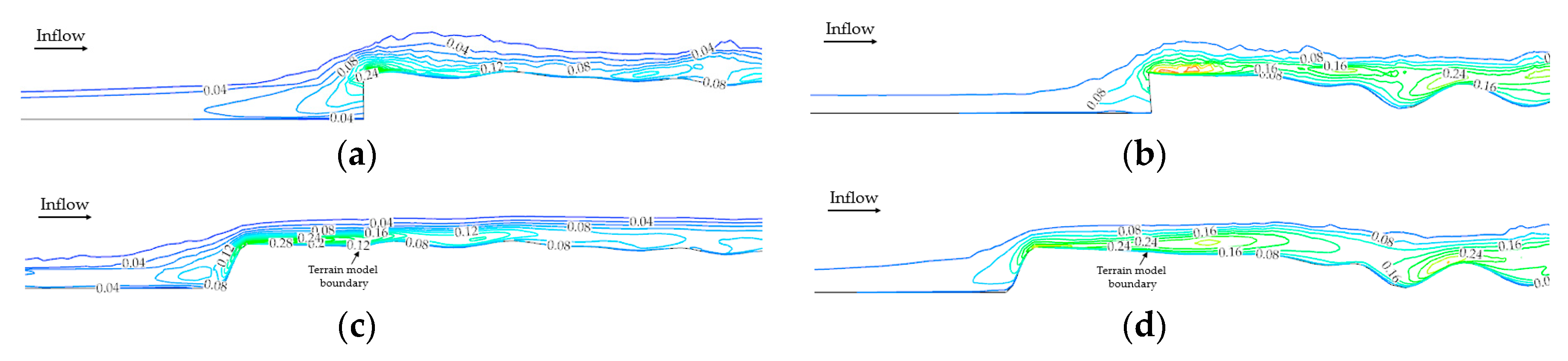
• The longitudinal wind speed ratio at different positions; namely, L/4, L/2 and 3L/4 of the bridge length, generally increase with height. The longitudinal wind speed ratio of the terrain model with BTS at L/4, L/2 and 3L/4 of the bridge length are larger than that of the terrain model without BTS for most cases.
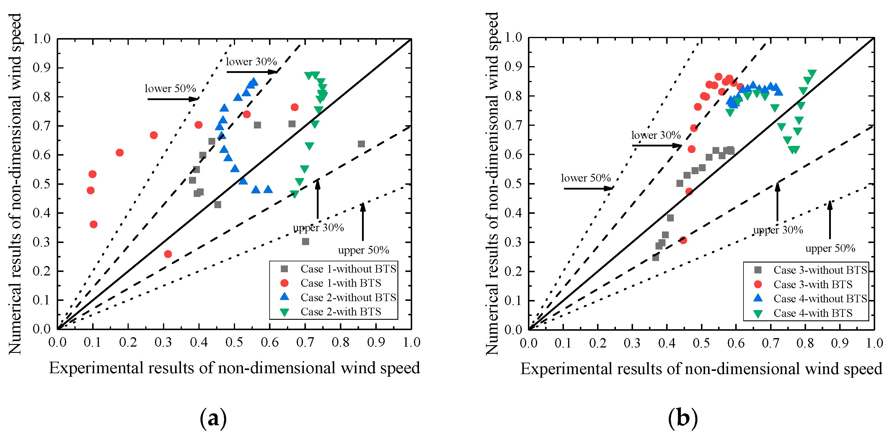
• In general, there are some discrepancies between the numerical results and wind tunnel tests results of wind characteristics, namely cross-bridge wind speed ratios, wind attack angles, and longitudinal wind speed ratios at L/4, L/2, and 3L/4 of the bridge length, but the maximum relative error between numerical and experimental results for most cases is about 30%.

References

1. Chock, G.Y.K.; Cochran, L. Modeling of topographic wind speed effects in Hawaii. J. Wind Eng. Ind. Aerodyn. 2005, 93, 623–638. [Google Scholar] [CrossRef]
2. Jackson, P.S.; Hunt, J.C.R. Turbulent wind flow over a low hill. Q. J. R. Meteorol. Soc. 1975, 101, 929–955. [Google Scholar] [CrossRef]
3. Hunt, J.C.R.; Leibovich, S.; Richards, K.J. Turbulent shear flows over low hills. Q. J. R. Meteorol. Soc. 1988, 114, 1435–1470. [Google Scholar] [CrossRef]
4. Li, Q.S.; Li, X.; He, Y.; Yi, J. Observation of wind fields over different terrains and wind effects on a super-tall building during a severe typhoon and verification of wind tunnel predictions. J. Wind Eng. Ind. Aerodyn. 2017, 162, 73–84. [Google Scholar] [CrossRef]
5. Harstveit, K. Full scale measurements of gust factors and turbulence intensity, and their relations in hilly terrain. J. Wind Eng. Ind. Aerodyn. 1996, 61, 195–205. [Google Scholar] [CrossRef]
6. Hannesen, R.; Dotzek, N.; Handwerker, J. Radar analysis of a tornado over hilly terrain on 23 July 1996. Phys. Chem. Earth Part B Hydrol. Ocean. Atmos. 2013, 25, 1079–2084. [Google Scholar] [CrossRef]
7. Lubitz, W.D.; White, B.R. Wind-tunnel and field investigation of the effect of local wind direction on speed-up over hills. J. Wind Eng. Ind. Aerodyn. 2007, 95, 639–661. [Google Scholar] [CrossRef]
8. Sharples, J.J.; Mcrae, R.H.D.; Weber, R.O. Wind characteristics over complex terrain with implications for bushfire risk management. Environ. Model. Softw. 2010, 25, 1099–1120. [Google Scholar] [CrossRef]
9. Abiven, C.; Palma, J.M.L.M.; Brady, O. High-frequency field measurements and time-dependent computational modelling for wind turbine siting. J. Wind Eng. Ind. Aerodyn. 2011, 99, 123–129. [Google Scholar] [CrossRef]
10. Risan, A.; Lund, J.A.; Chang, C.Y.; Sætran, L. Wind in complex terrain—Lidar measurements for evaluation of CFD simulations. Remote Sens. 2018, 10, 59. [Google Scholar] [CrossRef] [Green Version]
11. Lystad, T.M.; Fenerci, A.; Øiseth, O. Evaluation of mast measurements and wind tunnel terrain models to describe spatially variable wind field characteristics for long-span bridge design. J. Wind Eng. Ind. Aerodyn. 2018, 179, 558–573. [Google Scholar] [CrossRef]
12. Peng, Y.; Wang, S.; Li, J. Field measurement and investigation of spatial coherence for near-surface strong winds in Southeast China. J. Wind Eng. Ind. Aerodyn. 2018, 172, 423–440. [Google Scholar] [CrossRef]
13. Zhang, J.W.; Li, Q.S. Field measurements of wind pressures on a 600m high skyscraper during a landfall typhoon and comparison with wind tunnel test. J. Wind Eng. Ind. Aerodyn. 2018, 175, 391–407. [Google Scholar] [CrossRef]
14. Yu, C.; Li, Y.; Zhang, M.; Zhang, Y.; Zhai, G. Wind characteristics along a bridge catwalk in a deep-cutting gorge from field measurements. J. Wind Eng. Ind. Aerodyn. 2019, 186, 94–104. [Google Scholar] [CrossRef]
15. Jing, H.; Liao, H.; Ma, C.; Tao, Q.; Jiang, J. Field measurement study of wind characteristics at different measuring positions in a mountainous valley. Exp. Therm. Fluid Sci. 2020, 112, 1–18. [Google Scholar] [CrossRef]
16. Cermak, J.E. Physical modelling of flow and dispersion over complex terrain. Bound. Layer Meteorol. 1984, 30, 261–292. [Google Scholar] [CrossRef]
17. Xu, H.; He, Y.; Liao, H.; Ma, C.; Xian, R. Experiment of wind field in long-span bridge site located in mountainous valley terrain. J. Highw. Transp. Res. Dev. 2011, 7, 44–50. [Google Scholar]
18. Kozmar, H.; Allori, D.; Bartoli, G.; Borri, C. Complex terrain effects on wake characteristics of a parked wind turbine. Eng. Struct. 2016, 110, 363–374. [Google Scholar] [CrossRef]
19. Yan, B.W.; Li, Q.S. Coupled on-site measurement/CFD based approach for high-resolution wind resource assessment over complex terrains. Energy Convers. Manag. 2016, 117, 351–366. [Google Scholar] [CrossRef]
20. Mattuella, M.L.J.; Loredo-Souza, M.A.; Oliveira, G.K.M.; Petry, P.A. Wind tunnel experimental analysis of a complex terrain micrositing. Renewable Sustain. Energy Rev. 2016, 54, 110–119. [Google Scholar] [CrossRef]
21. Muhammad, J.C.; Horia, H. A hybrid approach for evaluating wind flow over a complex terrain. J. Wind Eng. Ind. Aerodyn. 2018, 175, 65–76. [Google Scholar] [CrossRef]
22. Kozmar, H.; Allori D.; Bartoli⁠, G.; Borri, G. Wind characteristics in wind farms situated on a hilly terrain. J. Wind Eng. Ind. Aerodyn. 2018, 174, 404–410. [Google Scholar] [CrossRef]
23. Chen, F.; Peng, H.; Chan, P.; Zeng, X. Low-level wind effects on the glide paths of the North Runway of HKIA: A wind tunnel study. Build. Environ. 2019, 164, 1–8. [Google Scholar] [CrossRef]
24. Flay, G.J.R.; King, A.B.; Revell, M.; Carpenter, P.; Turner, R.; Cenek, P.; Pirooz, A.A.S. Wind speed measurements and predictions over Belmont Hill, Wellington, New Zealand. J. Wind Eng. Ind. Aerodyn. 2019, 195, 1–18. [Google Scholar] [CrossRef]
25. Bowen, A.J. Modelling of strong wind flows over complex terrain at small geometric scales. J. Wind Eng. Ind. Aerodyn. 2003, 91, 1859–1871. [Google Scholar] [CrossRef]
26. Maurizi, A.; Palma, J.M.L.M.; Castro, F.A. Numerical simulation of the atmospheric flow in a mountainous region of the north of Portugal. J. Wind Eng. Ind. Aerodyn. 1998, 74–76, 219–228. [Google Scholar] [CrossRef]
27. Pang, J.; Song, J.; Lin, Z. Determination of design wind speed on bridge site over mountainous areas. China J. Highw. Transp. 2008, 21, 39–44. [Google Scholar]
28. Hu, P.; Li, Y.; Huang, G.; Kang, R.; Liao, H. The appropriate shape of the boundary transition section for a mountain gorge terrain model in a wind tunnel test. Wind Struct. 2015, 20, 15–36. [Google Scholar] [CrossRef]
29. Li, Y.; Hu, P.; Xu, X.; Qiu, J. Wind characteristics at bridge site in a deep-cutting gorge by wind tunnel test. J. Wind Eng. Ind. Aerodyn. 2017, 160, 30–46. [Google Scholar] [CrossRef]
30. Huang, G.; Cheng, X.; Peng, L.; Li, M. Aerodynamic shape of transition curve for truncated mountainous terrain model in wind field simulation. J. Wind Eng. Ind. Aerodyn. 2018, 178, 80–90. [Google Scholar] [CrossRef]
31. Hu, P.; Han, Y.; Xu, G.; Asce, M.A.; Li, Y.; Xue, F. Numerical Simulation of Wind Fields at the Bridge Site in Mountain-Gorge Terrain Considering an Updated Curved Boundary Transition Section. J. Aerosp. Eng. 2018, 31, 1–14. [Google Scholar] [CrossRef]
32. Liu, Z.; Chen, X.; Chen, Z. Optimization of Transition sections around terrain model at mountain canyon bridge site. China J. Highw. Transp. 2019, 32, 266–278. [Google Scholar]
33. Uchida, T.; Ohya, Y. Large-eddy simulation of turbulent airflow over complex terrain. J. Wind Eng. Ind. Aerodyn. 2003, 91, 219–229. [Google Scholar] [CrossRef]
34. Tong, H.; Walton, A.; Sang, J.; Chan, J.C.L. Numerical simulation of the urban boundary layer over the complex terrain of Hong Kong. Atmos. Environ. 2005, 39, 3549–3563. [Google Scholar] [CrossRef]
35. Deleon, R.; Sandusky, M.; Senocak, I. Simulations of turbulent flow over complex terrain using an immersed-boundary method. Bound. Layer Meteorol. 2018, 167, 399–420. [Google Scholar] [CrossRef]
36. Tamura, T.; Okuno, A.; Sugio, Y. LES analysis of turbulent boundary layer over 3D steep hill covered with vegetation. J. Wind Eng. Ind. Aerodyn. 2007, 95, 1463–1475. [Google Scholar] [CrossRef]
37. Cassiani, M.; Katul, G.G.; Albertson, J.D. The effects of canopy leaf area index on airflow across forest edges: Large-eddy simulation and analytical results. Bound. Layer Meteorol. 2008, 126, 433–460. [Google Scholar] [CrossRef] [Green Version]
38. Kim, H.G.; Patel, V.C.; Lee, C.M. Numerical simulation of wind flow over hilly terrain. J. Wind Eng. Ind. Aerodyn. 2000, 87, 45–60. [Google Scholar] [CrossRef]
39. Castellani, F.; Astolfi, D.; Burlando, M.; Terzi, L. Numerical modelling for wind farm operational assessment in complex terrain. J. Wind Eng. Ind. Aerodyn. 2015, 147, 320–329. [Google Scholar] [CrossRef]
40. Bitsuamlak, G.T.; Stathopoulos, T.; Bédard, C. Numerical evaluation of wind flow over complex terrain: Review. J. Aerosp. Eng. 2004, 17, 135–145. [Google Scholar] [CrossRef]
41. Yassin, M.F.; Al-Harbi, M.; Kassem, M.A. Computational fluid dynamics (CFD) simulations on the effect of rough surface on atmospheric turbulence flow above hilly terrain shapes. Environ. Forensics 2014, 15, 159–174. [Google Scholar] [CrossRef]
42. Yan, B.W.; Li, Q.S.; He, Y.C.; Chan, P.W. RANS simulation of neutral atmospheric boundary layer flows over complex terrain by proper imposition of boundary conditions and modification on the k-ε model. Environ. Fluid Mech. 2016, 16, 1–23. [Google Scholar] [CrossRef]
43. Wang, S.; Liu, X.; Lu, L. Simulation analysis of low-speed blow down wind tunnel with contraction curves. Mach. Tool Hydraul. 2012, 40, 100–104. [Google Scholar]
44. Huang, G.; Jiang, Y.; Peng, L.; Solari, G.; Liao, H.; Li, M. Characteristics of intense winds in mountain area based on field measurement: Focusing on thunderstorm winds. J. Wind Eng. Ind. Aerodyn. 2019, 190, 166–182. [Google Scholar] [CrossRef]
45. Tang, W. Quantitative techniques and weight allocation of evaluation indexes for complex systems. Sci. Technol. Process Policy 2009, 26, 116–118. [Google Scholar]
46. Ge, Y. Aerodynamic Design of Lupu Bridge in Shanghai. In Proceedings of the 3rd International Conference on Current and Future Trends in Bridge Design, Construction and Maintenance, Shanghai, China, 28–30 April 2003; pp. 69–80. [Google Scholar]
Figure 1. Schematic diagram of Artificial Cliffs.
Applsci 10 00751 g001
Figure 2. Terrain model BTS with/without horizontal straight line (Liu, et al., 2019). (a) BTS without horizontal straight line; (b) BTS with horizontal straight line.
Applsci 10 00751 g002
Figure 3. Elevation of the Xiangjiang Bridge and the mountainous terrain (Unit: cm). (a) Elevation of the Xiangjiang Bridge; (b) Complex terrain at the bridge site.
Applsci 10 00751 g003
Figure 4. Computational domain, boundary conditions, and grid of terrain model without BTS.
Applsci 10 00751 g004
Figure 5. Computational domain, boundary conditions and grid of terrain model with BTS.
Applsci 10 00751 g005
Figure 6. Schematic diagram of monitoring points. (a) Monitoring points at the main deck level; (b) Monitoring points profiles at L/4, L/2 and 3L/4 of the bridge length.
Applsci 10 00751 g006
Figure 7. Comparisons for average wind characteristics with different grid generations. (a) Mean cross-bridge wind speed at main deck level; (b) Wind attack angle at main deck level; (c) Longitudinal wind speed profiles at L/4, L/2 and 3L/4 of the bridge length.
Applsci 10 00751 g007
Figure 8. Mountainous terrain model with/without BTS in wind tunnel. (a) Terrain model without BTS; (b) Terrain model with BTS.
Applsci 10 00751 g008
Figure 9. Wind speed and turbulence intensity profiles at different height. (a) Wind speed profile; (b) Longitudinal turbulence intensity profile.
Applsci 10 00751 g009
Figure 10. Wind speed distribution along the inflow direction near the inlet of the terrain model without or with improved BTS from CFD simulation (unit: m/s). (a) Case 1 without BTS; (b) Case 2 without BTS; (c) Case 1 with BTS; (d) Case 2 with BTS.
Applsci 10 00751 g010
Figure 11. Turbulence kinetic energy distribution along the inflow direction near the inlet of the terrain model without or with improved BTS from CFD simulation (unit: m2s−2). (a) Case 1 without BTS; (b) Case 2 without BTS; (c) Case 1 with BTS; (d) Case 2 with BTS.
Applsci 10 00751 g011
Figure 12. Wind attack angle distribution along the inflow direction near the inlet of the terrain model without or with improved BTS from CFD simulation (unit: °). (a) Case 1 without BTS; (b) Case 2 without BTS; (c) Case 1 with BTS; (d) Case 2 with BTS.
Applsci 10 00751 g012
Figure 13. Non-dimensional cross-bridge wind speed at main deck level under different cases. (a) Case 1; (b) Case 2; (c) Case 3; (d) Case 4.
Applsci 10 00751 g013aApplsci 10 00751 g013b
Figure 14. Numerical results vs. experimental results of non-dimensional cross-bridge wind speed at main deck level under different cases. (a) Case 1 and 2; (b) Case 3 and 4.
Applsci 10 00751 g014
Figure 15. Wind attack angle at main deck level of wind tunnel tests and CFD simulation. (a) Case 1; (b) Case 2; (c) Case 3; (d) Case 4.
Applsci 10 00751 g015
Figure 16. Numerical results vs. experimental results of wind attack angles at main deck level under different cases. (a) Case 1 and 2; (b) Case 3 and 4.
Applsci 10 00751 g016
Figure 17. Numerical and experimental results of longitudinal wind speed ratio profiles at L/4.
Applsci 10 00751 g017
Figure 18. Numerical and experimental results of longitudinal wind speed ratio profiles at L/2.
Applsci 10 00751 g018
Figure 19. Numerical and experimental results of longitudinal wind speed ratio profiles at 3L/4.
Applsci 10 00751 g019
Figure 20. Numerical results vs. experimental results of longitudinal wind speed ratio at L/4 under different cases. (a) Case 1 and 2; (b) Case 3 and 4.
Applsci 10 00751 g020
Figure 21. Numerical results vs. experimental results of longitudinal wind speed ratio at L/2 under different cases. (a) Case 1 and 2; (b) Case 3 and 4.
Applsci 10 00751 g021
Figure 22. Numerical results vs. experimental results of longitudinal wind speed ratio at 3L/4 under different cases. (a) Case 1 and 2; (b) Case 3 and 4.
Applsci 10 00751 g022