Calibration of Large-Scale Spatial Positioning Systems Based on Photoelectric Scanning Angle Measurements and Spatial Resection in Conjunction with an External Receiver Array

Abstract

Positioning systems providing high-precision real-time measurements over very large spatial scales are urgently required for large-scale industrial manufacturing applications. While large-scale positioning systems (LSPSs) employing laser transmitter stations have been employed in engineering practice, the introduction of an LSPS into an existing industrial manufacturing setting must first solve the problems of docking with existing control points and external parameter calibration. However, calibrating the external parameters of a measurement system is very difficult under extreme and complicated working conditions due to the limited visibility of transmitter stations and the measurement distances involved. This problem is addressed in this paper by proposing a single transmitter station calibration method based on a photoelectric scanning multi-angle resection positioning model that combines photoelectric scanning angle measurements and spatial resection in conjunction with an external receiver array. Positioning information is obtained by solving the unknown parameters of the model according to a nonlinear optimization approach using the Levenberg–Marquardt least-squares fitting algorithm. The feasibility and spatial positioning accuracy of the proposed method are verified experimentally. The experimental results demonstrate that the principles of the proposed method are correct, and the method can achieve millimeter measurement accuracy, which meets the requirements of measurement tasks in engineering applications.

1. Introduction

Conventional metrology systems employed in industrial engineering applications typically provide real-time three-dimensional (3D) measurements over a range from millimeters to 10 m with precisions ranging from microns to sub-millimeters. In contrast, the standard measurement range of metrology systems employed in the fields of surveying and mapping is at least 100 m with precisions that are generally on the scale of millimeters or centimeters [1,2]. This discrepancy between the measurement ranges and precisions of these two metrology systems is acceptable when the scope of industrial engineering applications is limited in size to the measurement ranges provided by conventional metrology systems employed in industrial settings. However, the scope of industrial engineering applications has greatly expanded in recent years to include applications conducted within large uncontrollable spaces, such as aircraft assembly and large ship manufacturing, which has provided urgent motivation for the development of relatively high-precision metrology systems applicable to very large measurement spaces [3]. Meanwhile, the metrology systems employed in the fields of surveying and mapping have been developing progressively to facilitate automation and real-time measurements with increased precision. Accordingly, the measurement range and precision and other capabilities of these two metrology systems have been increasingly approaching each other over time based on similar measurement methodologies, resulting in a growing trend toward integration [4,5,6].

Recently, large-scale positioning systems (LSPSs), such as indoor global positioning systems (iGPSs) and workshop measuring and positioning systems (wMPSs), have been developed to provide 3D real-time dynamic industrial measurements based on photoelectric scanning [7,8]. These systems employ multiple laser transmitter stations distributed in the measurement space and several receivers located at the target points to be measured. Accordingly, these systems can simultaneously perform parallel measurements of multiple targets in a manner similar to that of the GPS resection principle. Moreover, the measurement range can be expanded by simply increasing the number of laser transmitter stations. Many LSPSs have been used in engineering practice at present. For example, the iGPS produced by Nikon provides indoor space measurements with an accuracy of 0.2 mm [9,10]. In addition, a concrete realization scheme and calibration method for wMPSs were proposed by Zhu et al. [11,12,13]. Meanwhile, the influence of wMPS network layout on location error was investigated by Zhi et al. [14], and the hardware and measurement algorithm employed in wMPSs have been optimized by Lao et al. [15,16].

While LSPSs employing laser transmitter stations have been employed in engineering practice, the introduction of an LSPS into an existing industrial manufacturing setting must first solve the problems of docking with existing control points and external parameter calibration. At present, the layout methods include the calibration of reference scale and calibration of control points. Both methods require two or more launch stations to complete the calibration [17,18]. There are three key factors to consider in layout; the first is effective measurement distance, the second is to ensure the rendezvous angles between launch stations, and the last is to ensure that all of the launch stations are visible to the target. However, in the local complex field measurement tasks, especially in the construction process, the site environment is complex, and it is difficult to ensure that multiple launch stations and the target point can be seen, which brings great inconvenience to the actual measurement. In addition, the layout calibration process of distributed measurement method is time-consuming and difficult. Therefore, aiming at the above problems, this paper takes a wMPS system as the research platform and proposes a flexible, single-station method for coordinate measurement. This method combines photoelectric scanning angle measurement sensing technology with the principle of spatial resection in photogrammetry in conjunction with an external receiver array [5,19]. Accordingly, the proposed calibration method avoids the limitations associated with a multi-station layout. Positioning information is obtained by solving the unknown parameters of the model according to a nonlinear optimization approach using the Levenberg–Marquardt least-squares fitting algorithm [20,21].

The remainder of this article is organized as follows. Section 2 presents the working principles and mathematical model of the wMPS. Section 3 presents a single station calibration model based on a combination of photoelectric scanning angle measurements and single image space resection in conjunction with an external receiver array, and the objective function solution process is discussed. The proposed approach is verified experimentally in Section 4. Finally, a brief overview of the work, concluding remarks, and a discussion of future research are presented in Section 5.

2. Laser Transmitter Measurement System

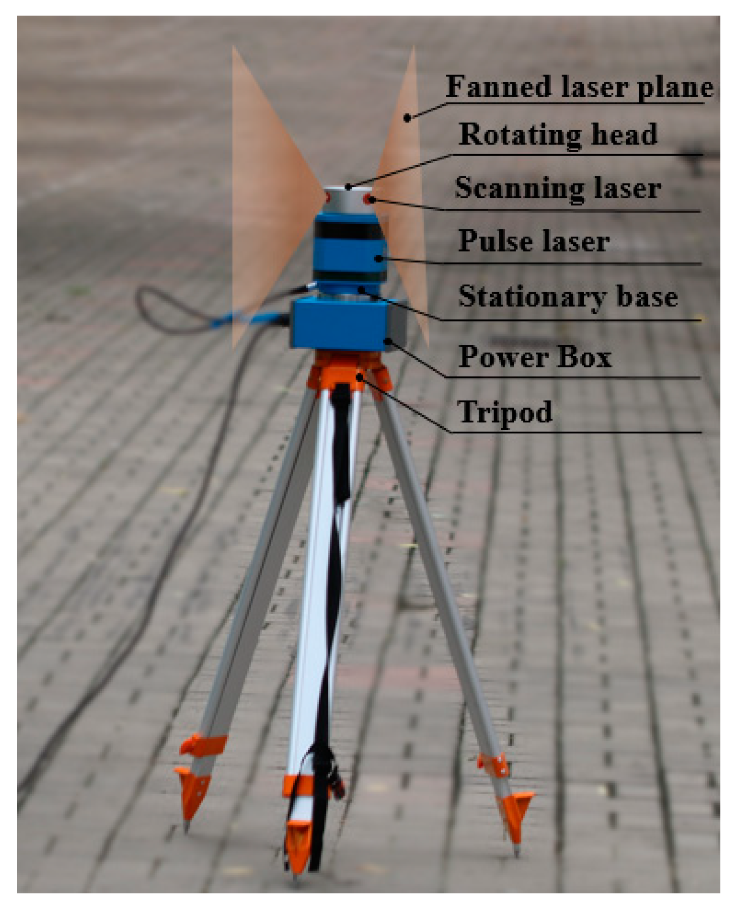
2.1. System Composition and Measurement Principles

A laser transmitter measurement system is primarily composed of a rotary-laser transmitter, a photoelectric receiver, and a terminal computer. As shown in Figure 1, the transmitter consists of a rotating head and a stationary base, where two laser modules capable of emitting fan-shaped laser beams are fixed on the rotating head at 90° angles, such that the optical axes of the laser modules are perpendicular to each other, and the tilt angles of the two planar laser beams relative to the rotating shaft are designed as +45° and −45°, respectively. The rotating head spins at a predefined rate in the anticlockwise direction, and the lasers accordingly scan the measurement space around the transmitter. Meanwhile, a pulsed laser is mounted on the stationary base, and emits a cyclical omnidirectional laser strobe synchronously as the head rotates to a predefined position each cycle. The photoelectric receiver is fixed at the target point, where it captures the synchronous laser strobe.

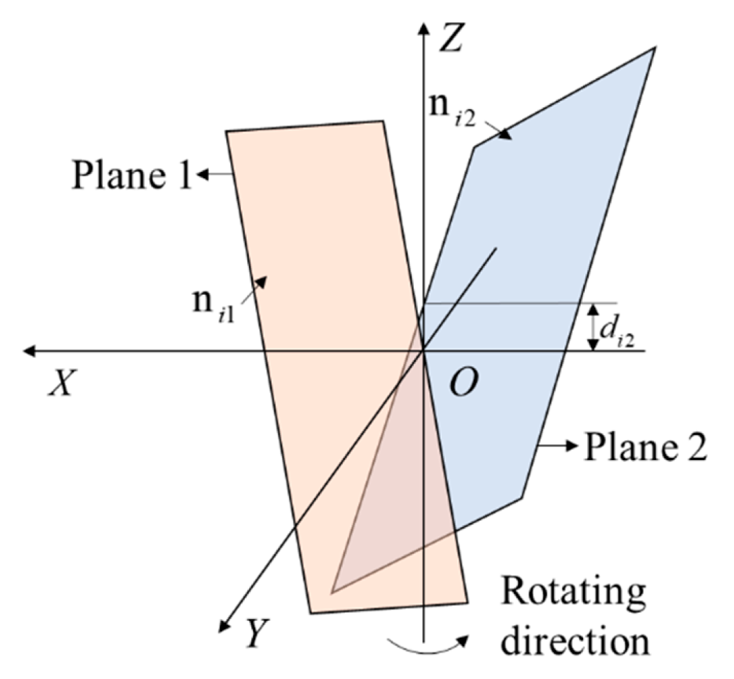
2.2. Single Transmitter Station Angle Measurement Model

As shown in Figure 2, the coordinate measurement model of the wMPS can be simplified into two rotary-laser fan-shaped planes 1 and 2, where the rotation axis of the two scanning laser planes is given as the Z axis, the intersection of plane 1 and the Z axis is defined as the origin O, the X axis initially lies in laser plane 1 and is perpendicular to the Z axis. The direction of the Y axis then follows from the standard right-hand rule of a Cartesian coordinate system.

The internal parameters of the transmitter (i.e., the initial plane parameters) are calibrated after the instrument is assembled, where the initial normal vectors of plane 1 and plane 2 are given as n_i1 = [a_i1 b_i1 c_i1]^T and n_i2 = [a_i2 b_i2 c_i2]^T, respectively, where i (i = 1, 2,…, N) is the transmitter number, and represents the position of the head at the first pulse signal, and $d_{i2}$ is the deviation between the two laser planes along the Z axis (Figure 2), which is caused by laser module assembly errors. Here, a_i1² + b_i1² + c_i1² = a_i2² + b_i2² + c_i2² = 1, such that n_i1 and n_i2 are both unit vectors. Accordingly, the equations of plane 1 and plane 2 can be expressed as follows.

$$\{\begin{array}{c}{a}_{i1}X+b_{i1}Y+c_{i1}Z+d_{i1}=0\\ a_{i2}X+b_{i2}Y+c_{i2}Z+d_{i2}=0\end{array}$$

(1)

When any laser plane sweeps across the receiver at position $M\left(X,Y,Z\right)$ over time, the relationship between the current plane parameters $\left(a_{ij}^{\prime },b_{ij}^{\prime },c_{ij}^{\prime },d_{ij}^{\prime }\right)$, where j is an integer ranging from 1 to 2, and represents the times when the receiver at $M\left(X,Y,Z\right)$ receives signals from planes 1 and 2, respectively, and the initial plane parameters can be expressed as follows.

$$\left[\begin{array}{c}{a}_{ij}^{\prime }\\ b_{ij}^{\prime }\\ c_{ij}^{\prime }\\ d_{ij}^{\prime }\end{array}\right]=\left[\begin{array}{cc}R\left({\theta }_j\right)& 0\\ 0& 1\end{array}\right]\left[\begin{array}{c}{a}_{ij}\\ b_{ij}\\ c_{ij}\\ d_{ij}\end{array}\right]$$

(2)

$$R\left({\theta }_j\right)=\left[\begin{array}{ccc}\cos \left({\theta }_j\right)& -\sin \left({\theta }_j\right)& 0\\ \sin \left({\theta }_j\right)& \cos \left({\theta }_j\right)& 0\\ 0& 0& 1\end{array}\right]$$

(3)

here, ${\theta }_j$ is the angle of rotation of the plane from its initial position to the receiver, which is calculated as follows. When the head returns to its initial position, the receiver receives the pulse signal at a time recorded as $t_0$. When the head rotates to ${\theta }_1$, the receiver receives the signal from laser plane 1 and records the time as $t_1$. When the head rotates to ${\theta }_2$, the receiver receives the light signal from laser plane 2 and records the time as $t_2$. Finally, when the head again rotates to its initial position, the time is recorded as $t_0^{\prime }$. As a result, $T=t_0^{\prime }-t_0$ is the rotational period of the transmitter, which has been calibrated at the time of manufacture. Assuming that the head rotates with an angular velocity ω, ${\theta }_j$ will be obtained as follows:

$${\theta }_j=\omega (t_j-t_0)=\frac{2\pi (t_j-t_0)}{(t_0^{\prime }-t_0)}$$

here, $t_{1j}=t_j-t_0$ is the minimum time interval from the initial position to the receiver. Therefore, ${\theta }_j$ can be expressed according to t_1j and T as follows:

$${\theta }_j=\frac{t_{1j}}{T}\times 2\pi$$

(4)

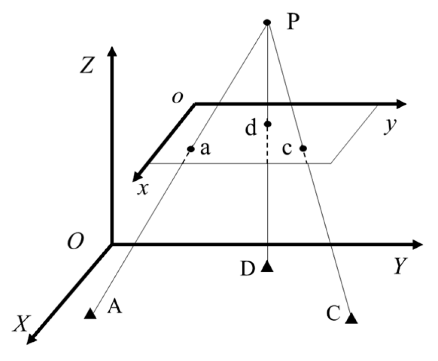
2.3. Space Resection

The principle of space resection, which is also denoted as single image space resection, is illustrated in Figure 3. Here, the points a, b, and c in the image coordinate system respectively correspond with the predetermined ground coordinates of control points A, B, and C on the ground, and the exterior orientation element of the image at the moment of aerial photography is solved according to the collinear conditional Equation [22].

3. Single Transmitter Station Calibration Method

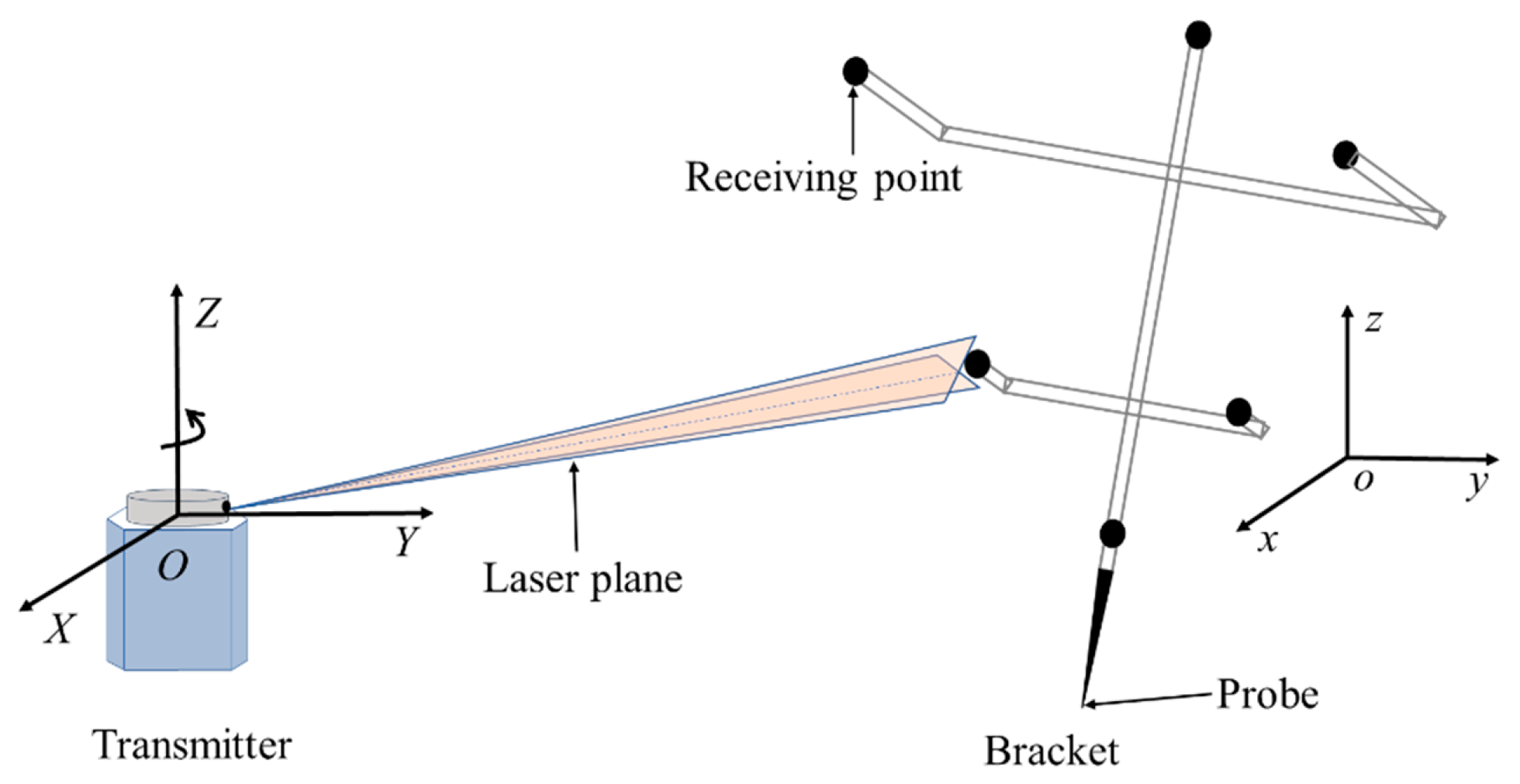
3.1. Photoelectric Scanning Multi-Angle Resection Positioning

The positioning of a single laser transmitter can be calibrated based on a combination of photoelectric scanning angle measurements and single image space resection using a pre-designed receiver array, as illustrated in Figure 4. Here, the laser transmitter can be regarded as a fixed position camera, and the receiver array includes a fixed number of photoelectric receivers mounted at known positions within a receiver array coordinate system o-xyz with its origin (i.e., the probe point) placed in constant contact with a known measurement point within the transmitter station coordinate system O-XYZ. These receivers serve as control points in the array coordinate system with corresponding points in the transmitter station coordinate system. Then, the photoelectric scanning multi-angle resection positioning equation can be established according to the scanning angle information measured by each receiver on the receiver array. A sufficient number of control points on the receiver array provide for a sufficient number of spatial geometric constraints to solve the rotational and translational relationships between array coordinate system o-xyz and transmitter station coordinate system O-XYZ to achieve spatial positioning.

The array coordinate frame o-xyz can be regarded as a coordinate frame lying intermediate with the transmitter coordinate frame O-XYZ defined in Figure 2, and the origin of the array frame and the coordinates of the control points in o-xyz are known structural parameters. The rotation of the transmitter station head then yields the scanning angle information measured for each receiver on the receiver array in the O-XYZ coordinate frame based on Equation (1). A similar scanning angle equation can also be obtained for each receiver mounted on the receiver array. Therefore, the photoelectric scanning multi-angle resection positioning model of the O-XYZ frame and the o-xyz frame can be established by combining the above measurement information. The model is then applied to obtain positioning information based on a least-squares optimization approach.

3.2. Positioning Optimization Equation

The coordinates of receivers at any point within the O-XYZ frame are denoted as (X, Y, Z), the corresponding coordinates in the o-xyz frame are denoted as (x, y, z), and R and T are the respective rotation and translation matrices that relate (x, y, z) to (X, Y, Z) as follows.

$$\left[\begin{array}{c}X\\ Y\\ Z\end{array}\right]=R\cdot \left[\begin{array}{c}x\\ y\\ z\end{array}\right]+T$$

(5)

$$R=\left[\begin{array}{ccc}{r}_1& r_2& r_3\\ r_4& r_5& r_6\\ r_7& r_8& r_9\end{array}\right]$$

(6)

$$T=\left[\begin{array}{c}{t}_1\\ t_2\\ t_3\end{array}\right]$$

(7)

In addition, we note that R in Equation (6) is an orthogonal matrix. Substituting Equation (5) into Equation (1) yields the following.

$$\left[{\begin{array}{ccc}{a}_{ij}& b_{ij}& c\end{array}}_{ij}\right]\cdot \left[\begin{array}{c}{r}_{1}x+r_{2}y+r_{3}z+t_1\\ r_{4}x+r_{5}y+r_{6}z+t_2\\ r_{7}x+r_{8}y+r_{9}z+t_3\end{array}\right]+d_{ij}=0$$

(8)

The scanning process of the two fan-shaped lasers on the head provide two plane Equations (8) for each control point. Therefore, N control points obtain 2N plane equations given by Equation (8). Accordingly, this includes nine rotation parameters r_l, l = 1, 2, …, 9, and three translation parameters t₁, t₂, and t₃, resulting in a total of 9 + 3 = 12 unknown parameters. Obtaining these 12 parameters would yield the coordinates of the individual receivers mounted on the array in the O-XYZ frame. This solution process is configured as follows.

Setting the distance between the control point and the two laser planes as $e_{ij}$, yields the following.

$$e_{ij}=\frac{a_{ij}X+b_{ij}Y+c_{ij}Z+d_{ij}}{\sqrt{a_{ij}{}^2+b_{ij}{}^2+c_{ij}{}^2}}$$

(9)

This can be rewritten according to Equations (5) and (8) as follows.

$$e_{ij}=\left[{\begin{array}{ccc}{a}_{ij}& b_{ij}& c\end{array}}_{ij}\right]\cdot \left[\begin{array}{c}{r}_{1}x+r_{2}y+r_{3}z+t_1\\ r_{4}x+r_{5}y+r_{6}z+t_2\\ r_{7}x+r_{8}y+r_{9}z+t_3\end{array}\right]+d_{ij}$$

(10)

Then, Formula (10) can be expanded for the k-th receiver, k = 1, 2, …, N, mounted on the receiver array as follows.

$$\begin{array}{l}{e}_{ijk}=a_{ij}{r}_1{x}_k+a_{ij}{r}_2{y}_k+a_{ij}{r}_3{z}_k+a_{ij}{t}_1+b_{ij}{r}_4{x}_k+b_{ij}{r}_5{y}_k\\ +b_{ij}{r}_6{z}_k+b_{ij}{t}_2+c_{ij}{r}_7{x}_k+c_{ij}{r}_8{y}_k+c_{ij}{r}_9{z}_k+c_{ij}{t}_3+d_{ij}\end{array}$$

(11)

However, in practical applications, determining R by this method does not in general satisfy the orthogonal constraint condition. Therefore, we adopt a nonlinear method to determine R and T. In this method, the elements in Equation (11) satisfy the following orthogonal constraint conditions.

$$\{\begin{array}{l}{f}_1=r_1^2+r_2^2+r_3^2-1=0\\ f_2=r_4^2+r_5^2+r_6^2-1=0\\ f_3=r_7^2+r_8^2+r_9^2-1=0\\ f_4=r_1{r}_4+r_2{r}_5+r_3{r}_6=0\\ f_5=r_1{r}_7+r_2{r}_8+r_3{r}_9=0\\ f_6=r_4{r}_7+r_5{r}_8+r_6{r}_9=0\end{array}$$

(12)

Accordingly, we obtain the unknown elements in R and T by employing (12) as penalty constraints in the following nonlinear optimization algorithm:

$$F=\min \left\{{\displaystyle \sum {\displaystyle \sum e_{ijk}^2+\mu {\displaystyle \sum _{m=1}^6{f}_m^2}}}\right\}$$

(13)

where $\mu$ is a penalty factor. The solution of Equation (13) yields (X, Y, Z) from Equation (5) based on the known values of (x, y, z).

3.3. Optimization Solution Method and Initial Value Estimates

Because Equation (13) is nonlinear, the solution to the objective function is considered to be an unconstrained nonlinear optimization problem. In addition, a least-squares equation of these 12 unknown parameters can be solved when N ≥ 6. The Levenberg–Marquardt algorithm is considered one of the most effective nonlinear least squares algorithms available owing to its advantages of rapid convergence and high stability. Therefore, this algorithm is employed in the present work to solve Equation (13). Because the Levenberg–Marquardt algorithm is a least-squares fitting method, its calculation process first selects appropriate initial values of the 12 unknown parameters, and then calculates their values step by step according to established iteration rules until their true values are approached to within an established tolerance.

Defining the vectors J₉ = [r₁ r₂ r₃ r₄ r₅ r₆ r₇ r₈ r₉ t₁ t₂ t₃]^T and J₃ = [r₇ r₈ r₉]^T allows Equation (8) to be expressed as in the following matrix form:

$$U{J}_9+V{J}_3+D=0$$

(14)

where U is a 2N × 9 matrix, V is a 2N × 3 matrix, and D is a 2N × 1 matrix, which are defined as follows.

$$U=\left[\begin{array}{ccccccccc}{a}_{11}{x}_k& a_{11}{y}_k& a_{11}{z}_k& b_{11}{x}_k& b_{11}{y}_k& b_{11}{z}_k& a_{11}& b_{11}& c_{11}\\ a_{12}{x}_k& a_{12}{y}_k& a_{12}{z}_k& b_{12}{x}_k& b_{12}{y}_k& b_{12}{z}_k& a_{12}& b_{12}& c_{12}\\ ⋮& ⋮& ⋮& ⋮& ⋮& ⋮& ⋮& ⋮& ⋮\\ ⋮& ⋮& ⋮& ⋮& ⋮& ⋮& ⋮& ⋮& ⋮\\ a_{N1}{x}_k& a_{N1}{y}_k& a_{N1}{z}_k& b_{N1}{x}_k& b_{N1}{y}_k& b_{N1}{z}_k& a_{N1}& b_{N1}& c_{N1}\\ a_{N2}{x}_k& a_{N2}{y}_k& a_{N2}{z}_k& b_{N2}{x}_k& b_{N2}{y}_k& b_{N2}{z}_k& a_{N2}& b_{N2}& c_{N2}\end{array}\right]$$

$$V=\left[\begin{array}{ccc}{c}_{11}{x}_1& c_1{y}_1& c_1{z}_1\\ c_{12}{x}_1& c_2{y}_1& c_2{z}_1\\ ⋮& ⋮& ⋮\\ ⋮& ⋮& ⋮\\ c_{N1}{x}_k& c_{N1}{y}_k& c_{N1}{z}_k\\ c_{N2}{x}_k& c_{N2}{y}_N& c_{N2}{z}_k\end{array}\right]$$

$$D={\left[d_{i1},d_{i2},\dots d_{i1},d_{i2}\right]}^{\mathrm{T}}$$

Because plane 1 passes through O, we know that $d_{i1}=0$. In addition, $d_{i2}$ is relatively small owing to laser module assembly adjustment. Therefore, the initial values of the elements of D can be set to 0. This simplifies Equation (14) as

$$U{J}_9+V{J}_3=0$$

(15)

It is also known from constraints (12) that r₇, r₈, and r₉ satisfy the constraint condition $f_3=r_7^2+r_8^2+r_9^2-1=0$, which indicates that

$$J_3^{\mathrm{T}}{J}_3-1=0$$

(16)

Therefore, the initial values of the 12 unknown parameters in Equation (13) can be selected as

$$F_0={\left(U{J}_9+V{J}_3\right)}^{\mathrm{T}}\left(U{J}_9+V{J}_3\right)+\lambda \left(J_3^T{J}_3-1\right)$$

(17)

where $\lambda$ is the Lagrange multiplier. Minimization over successive iterations is determined by obtaining the partial derivatives of F₀ with respect to J₉ and J₃, and setting $\frac{\partial F_0}{\partial J_9}=0$ and $\frac{\partial F_0}{\partial J_3}=0$. This yields the following set of matrix equations:

$$\left(Q-\lambda I\right)J_3=0$$

(18)

where

$$Q=V^{\mathrm{T}}\left(I-U{\left(U^{\mathrm{T}}U\right)}^{-1}{U}^{\mathrm{T}}\right)V$$

(19)

and

$$J_9=-{\left(U^{T}U\right)}^{-1}{U}^{\mathrm{T}}V{J}_3$$

(20)

It is known from Equation (19) that Q is a positive definite matrix. In addition, it is known from Equation (18) that $\lambda$ is the minimum eigenvalue of Q, while it is known from Equations (16) and (18) that J₃ is the eigenvector of Q corresponding to $\lambda$. Finally, J₉ can be obtained from Equation (20).

4. Verification Experiments

4.1. Experimental Setup

The feasibility and measurement accuracy of the proposed positioning method was validated by arranging a single laser transmitter station in an outdoor space with dimensions of about 30 m × 30 m. The structural parameters (internal parameters) of the transmitter station used in the experiments are listed in

Table 1. Parameters of the laser planes of the transmitter station employed for verification testing, where a_j, b_j, c_j, and d_j are the parameters of Equation (1).

Plane NO.	1				2
Parameter	a1	b1	c1	d1	a2	b2	c3	d2
Value	0	−0.432757	0.901510	0	−0.757457	0.00227	0.652880	0.166872

. The multipoint receiver array employed during verification testing is shown in Figure 5.

The receiver positions (i.e., control points) and probe position of the receiver array must be calibrated in advance. Considering that a millimeter precision level is sufficient in engineering applications, the receiver array can be calibrated using the positional parameters obtained from the wMPS. However, the probe coordinates cannot be measured by directly installing the receiver. Therefore, the distance constraint method was used to measure the probe coordinates. This can be conducted with a high degree of precision by keeping the probe in contact with a fixed target point and changing the posture of the receiver array multiple times to obtain the coordinates of the control points in different postures. Accordingly, the multiple different coordinates can be used in the least square method under over-determined conditions to obtain the spatial 3D coordinates of the probe and control points based on the fact that the distances between the control points and the probe are constant. The obtained positions of the control points in the o-xyz frame are listed in

Table 2. Calibration results of the receiver array in Figure 5 (unit: mm). Here, the probe point is defined as the origin of the o-xyz frame. The direction from the probe to P0 is defined as the z axis. A line perpendicular to the z axis and passing through P1 is defined as the x axis. The direction of the y axis is defined according to the right-hand rule.

Point ID	x	y	z
P0	0.00	0.00	−943.99
P1	356.30	0.00	−771.45
P2	−221.69	−277.46	−771.68
P3	193.48	−9.92	−442.30
P4	−112.68	−157.93	−441.85
P5	0.41	−0.05	−371.92
Probe	0.00	0.00	0.00

based on the probe point being defined as the origin, where the direction from the probe to P₀ is defined as the z axis, a line perpendicular to the z axis and passing through P₁ is defined as the x axis, and the direction of the y axis is defined according to the right-hand rule.

4.2. Estimation and Analysis of the Experimental Data

To verify the feasibility and measurement accuracy of the positioning method, two schemes are adopted to verify the model. The first method is to self-verify the measurement results under different attitude of the same target point, and the second is to use total station to verify the measured data.

4.2.1. Self-verification the Measurement Results

The accuracy of the proposed method was evaluated by acquiring multiple measurements of a single target point in a known position relative to the transmitter station with the receiver array held in constant contact under four different postures. Theoretically, the coordinate values in the O-XYZ frame obtained in this process should be equivalent for all postures because the position of the probe never changes.

The values of the conversion parameters r_l, l = 1, 2, …, 9, and t₁, t₂, and t₃ obtained with the receiver array held in the four different postures are listed in

Table 3. Conversion parameters for transforming between the o-xyz frame and the O-XYZ frame with the shaped receiver array held in four different postures.

Posture	1	2	3	4
r1	−0.87051125	−0.79116910	−0.77006598	−0.71680738
r2	0.45422411	0.45022282	0.51670999	0.58164049
r3	0.18944815	0.41394549	−0.37417830	−0.38455397
r4	0.32510523	0.53599181	0.61074966	0.68063671
r5	0.81972864	0.83638869	0.76657725	0.70342008
r6	−0.47154174	0.11474707	−0.19835402	−0.20477787
r7	−0.36948175	−0.29455764	0.18434507	0.15139587
r8	−0.34889166	0.31265615	−0.38127457	−0.40852700
r9	−0.86125362	−0.90304030	−0.90589527	−0.90010200
t1	7862.72	7366.73	6177.68	5561.38
t2	−4845.74	−6228.05	−7190.85	−7774.33
t3	3074.98	1337.52	−2220.50	−1858.96

. As expected, these values generally vary considerably for the different array postures adopted. The coordinate values of the target point in the O-XYZ frame obtained with the receiver array held in the four different postures and their deviations from the true coordinate values are listed in

Table 4. Measured X, Y, and Z coordinate values (unit: mm) and their deviations from the true values with the external receiver array held in four different postures. Here, ΔL = √(ΔX² + ΔY² + ΔZ²).

Posture	X	Y	Z	∆X	∆Y	∆Z	∆L
1	9556.1	1473.6	−1126.2	−2.5	−0.4	0.3	2.6
2	9560.5	1474.2	−1126.9	1.7	0.3	−0.5	1.8
3	9558.4	1473.7	−1126.3	−0.1	−0.3	0.2	0.4
4	9559.5	1474.4	−1126.6	0.9	0.5	−0.1	1.0
Average	9558.6	1474.0	−1126.5	1.3	0.4	0.3	1.5

, where $\mathsf{\Delta }L=\sqrt{\mathsf{\Delta }{X}^2+\mathsf{\Delta }{Y}^2+\mathsf{\Delta }{Z}^2}$ is the spatial difference between the true and measured target points. It can be seen from the table that the single transmitter station system using the external receiver array generally obtains a greater error in the X-axis direction than in the other directions, and the maximum error obtained was 2.5 mm, while ΔL was not greater than 2.6 mm.

Because the positions of each control point were directly obtained using the wMPS, and the precision is sub-millimeter [18], we can then consider that the error of the single transmitter station system is mainly caused by calibration error.

4.2.2. Accuracy Verification Experiment

A Leica TCL1201+ electronic total station (with the accuracy of angle measurement of ±1 and that of distance measurement of ± (1 mm + 1.5 × 10⁻⁶ D)) were installed to verify the measured data. Two sets of data were obtained by measuring 14 control points in the test site with total station (RTS) and receiver array single station system (RASS). Three points were selected to obtain the transformation parameters (see

Table 5. Conversion parameters from the receiver array single station system (RASS) coordinate system to the total station (RTS) coordinate system, where ∆X, ∆Y, and ∆Z are translation parameters, and ∆α, ∆β, and ∆γ are rotation parameters; K is a scale factor.

Parameter	∆X	∆Y	∆Z	∆α	∆β	∆γ	K
Value	113,526.6	97,152.5	8704.9	−0.0240148	−0.028201	0.889006	0.99880

) from the coordinate system of the launching station to that of the total station. The other 11 points measured by the single transmitting station were changed to the coordinate system of the total station as the verification points by transforming the parameters.

Comparison results are shown in

Table 6. Coordinate differences of verification points from (RTS) and (RASS) (mm), where DX, DY, and DZ are the differences of coordinates. Here, ΔL = √(ΔX² + ΔY² + ΔZ²).

Point Name	Method	X	Y	Z	DX	DY	DZ	ΔL
1	RTS	106,367.8	103,597.0	10,061.9	0.8	1.5	−1.6	2.3
	RASS	106,367.0	103,595.5	10,063.5
2	RTS	106,166.7	105,443.3	10,060.8	−1.5	1.9	1.6	2.9
	RASS	106,168.2	105,441.4	10,059.2
3	RTS	106,156.3	106,285.1	10,071.0	−0.7	1.5	−2.1	2.7
	RASS	106,157.0	106,283.6	10,073.1
4	RTS	108,045.9	108,595.1	10,092.2	2.0	2.5	1.9	3.7
	RASS	108,043.9	108,592.6	10,090.3
5	RTS	109,667.7	107,222.4	10,097.9	0.9	−2.8	−0.9	3.1
	RASS	109,666.8	107,225.2	10,098.8
6	RTS	108,026.8	105,480.6	10,086.4	−0.6	1.6	−2.0	2.6
	RASS	108,027.4	105,479.0	10,088.4
7	RTS	112,321.8	104,221.2	10,079.4	−1.3	1.1	−1.8	2.5
	RASS	112,323.1	104,220.1	10,081.2
8	RTS	122,829.8	93,402.2	10,026.6	0.0	0.8	1.0	1.3
	RASS	122,829.8	93,401.4	10,025.6
9	RTS	126,278.7	96,203.8	10,097.0	1.9	2.4	−2.4	3.9
	RASS	126,276.8	96,201.4	10,099.4
10	RTS	110,704.1	102,478.5	10,061.2	1.7	0.6	1.8	2.5
	RASS	110,702.4	102,477.9	10,059.4
11	RTS	110,464.1	105,179.0	10,084.5	1.2	−1.7	−1.2	2.5
	RASS	110,462.9	105,180.7	10,085.7
	Average				0.4	0.8	−0.5	2.7

, where DX, DY, and DZ are the differences of coordinates, ∆L denotes the location difference, and $\mathsf{\Delta }L=\sqrt{\mathsf{\Delta }{X}^2+\mathsf{\Delta }{Y}^2+\mathsf{\Delta }{Z}^2}$ represents the average value of absolute value of each difference. It can be seen from the Table 6 that the single transmitter station system using the external receiver array generally obtained a greater error at points 4 and 9, both of which are farthest from the launch site, and the maximum error obtained was −2.8 mm, while ∆L was not greater than 3.9 mm. That means, with increasing distance from the target to the launch station, the accuracy of the receiver array single station system becomes lower. This is consistent with the measurement error distribution of wMPS.

Therefore, the experimental results clearly demonstrate that the single station calibration method based on the receiver array proposed in this paper is entirely feasible, and the proposed solution method of the measurement model is correct and effective.

5. Conclusions

While LSPSs employing laser transmitter stations have been employed in engineering practice, the introduction of an LSPS into an existing industrial manufacturing setting must first solve the problems of docking with existing control points and external parameter calibration. However, calibrating the external parameters of a measurement system is very difficult under extreme and complicated working conditions due to the limited visibility of transmitter stations and the measurement distances involved. This problem was addressed here by proposing a single transmitter station calibration method based on a photoelectric scanning multi-angle resection positioning model that combines photoelectric scanning angle measurements and spatial resection in conjunction with an external receiver array. Positioning information is then obtained by solving the unknown parameters of the model according to a nonlinear optimization approach using the Levenberg–Marquardt least-squares fitting algorithm. Two approaches were used to verify the feasibility and measurement accuracy of the positioning method. The experimental results demonstrated that the principles of the proposed method are correct, and the method can achieve millimeter measurement accuracy, which meets the requirements of measurement tasks in engineering applications. Compared with existing photoelectric scanning multi-station calibration methods, the proposed single transmitter station method avoids the limitations associated with a multi-station layout. The introduction of a local positioning system into the engineering metrology field proposed in this paper is of great practical significance because it inherits the characteristics of multi-tasking, high precision, and real-time measurements inherent in photoelectric scanning technology. Additional research is required in the future, such as developing a method for improving the measurement precision and reducing the effect of external receiver array attitude on the measurement accuracy.

References

1. Shenghua, Y.E.; Zhong, W.; Xinghua, Q. Review and prospect of precision inspection. China Mech. Eng. 2000, 11, 262–263. [Google Scholar]
2. Xiong, C.B.; Bai, H.Z.; Li, L.; Zhu, J.G. Self-location method of regional positioning system in engineering survey application. J. Tongji Univ. Nat. Sci. 2017, 45, 1879–1886. [Google Scholar]
3. Li, W.; Fang, W.; Hongwen, X. Implementation of measurement method for large scale roomage. J. Nanjing Univ. Aeronaut. Astronaut. 2012, 44, 48. [Google Scholar]
4. Ye, S.H.; Zhu, J.G.; Zhang, Z.L.; Zhou, H.; Guo, L. Status and development of large-scale coordinate measurement research. ACTA Metrol. Sin. 2008, 29, 1–6. [Google Scholar]
5. Cuypers, W.; Gestel, N.V.; Voet, A.; Kruth, J.P.; Mingneau, J.; Bleys, P. Optical measurement techniques for mobile and large-scale dimensional metrology. Opt. Lasers Eng. 2009, 47, 292–300. [Google Scholar] [CrossRef] [Green Version]
6. Peggs, G.N.; Maropoulos, P.G.; Hughes, E.B.; Forbes, A.B.; Robson, S.; Ziebart, M.; Muralikrishnan, B. Recent developments in large-scale dimensional metrology. J. Eng. Manuf. B 2009, 223, 571–595. [Google Scholar] [CrossRef]
7. Maisano, D.A.; Jamshidi, J.; Franceschini, F.; Maropoulos, P.G.; Mastrogiacomo, L. Indoor GPS: System functionality and initial performance evaluation. Int. J. Manuf. Res. 2008, 3, 335–349. [Google Scholar] [CrossRef]
8. Yang, L.; Yang, X.; Zhu, J.; Duan, M.; Lao, D. Novel method for spatial angle measurement based on rotating planar laser beams. Chin. J. Mech. Eng. Engl. Ed. 2010, 6, 758. [Google Scholar] [CrossRef]
9. Maisano, D.A.; Jamshidi, J.; Franceschini, F.; Maropoulos, P.G.; Mastrogiacomo, L.; Mileham, A.R.; Owen, G.W. A comparison of two distributed large-volume measurement systems: The mobile spatial co-ordinate measuring system and the indoor global positioning system. Proc. Inst. Mech. Eng. Part B J. Eng. Manuf. 2009, 223, 511–521. [Google Scholar] [CrossRef]
10. Wang, Z.; Mastrogiacomo, L.; Franceschini, F.; Maropoulos, P. Experimental comparison of dynamic tracking performance of iGPS and laser tracker. Int. J. Adv. Manuf. Technol. 2011, 56, 205–213. [Google Scholar] [CrossRef] [Green Version]
11. Xiong, Z.; Zhu, J.G.; Zhao, Z.Y.; Yang, X.Y.; Ye, S.H. Workspace measuring and positioning system based on rotating laser planes. Mechanika 2012, 18, 94–98. [Google Scholar] [CrossRef] [Green Version]
12. Lao, D.; Yang, X.; Zhu, J.; Yang, L. Study on calibration technology of network laser scan space positioning system. J. Mech. Eng. 2011, 47, 1–6. [Google Scholar] [CrossRef]
13. Zhao, Z.; Zhu, J.; Xue, B.; Yang, L. Optimization for calibration of large-scale optical measurement positioning system by using spherical constraint. JOSA A 2014, 31, 1427–1435. [Google Scholar] [CrossRef] [PubMed]
14. Zhi, X.; Zhu, J.; Lei, G.; Geng, L.; Ren, Y.; Yang, X.Y.; Ye, S.H. Verification of angle measuring uncertainty for workspace measuring and positioning system. Chin. J. Sens. Actuat. 2012, 25, 229–235. [Google Scholar]
15. Lao, D.B.; Yang, X.Y.; Zhu, J.G.; Ye, S.H. Optimization of calibration method for scanning planar laser coordinate measurement system. Opt. Precis. Eng. 2011, 19, 870–877. [Google Scholar]
16. Guo, S.; Lin, J.; Ren, Y.; Shi, S.; Zhu, J. Application of a self-compensation mechanism to a rotary-laser scanning measurement system. Meas. Sci. Technol. 2017, 28, 115007. [Google Scholar] [CrossRef] [Green Version]
17. Yang, L.H.; Zhu, J.G.; Zhang, G.J.; YE, S.H. Orientation method for workspace measurement positioning system based on scale bar. J. Tianjin Univ. 2012, 45, 814–819. [Google Scholar]
18. Zhao, Z.; Zhu, J.; Lin, J.; Yang, L.; Xue, B.; Xiong, Z. Transmitter parameter calibration of the workspace measurement and positioning system by using precise three-dimensional coordinate control network. Opt. Eng. 2014, 53, 084108. [Google Scholar] [CrossRef]
19. Zhang, X.; Zhu, Z.; Yuan, Y.; Li, L.; Sun, X.; Yu, Q.; Ou, J. A universal and flexible theodolite-camera system for making accurate measurements over large volumes. Opt. Lasers Eng. 2012, 50, 1611–1620. [Google Scholar] [CrossRef]
20. Levenberg, K. A method for the solution of certain non-linear problems in least squares. J. Heart Lung Transplant. Off. Publ. Int. Soc. Heart Transplant. 1944, 31, 436–438. [Google Scholar] [CrossRef] [Green Version]
21. Marquardt, D.W. An algorithm for least-squares estimation of nonlinear parameters. J. Soc. Ind. Appl. Math. 1963, 11, 431–441. [Google Scholar] [CrossRef]
22. Easa, S.M. Space resection in photogrammetry using collinearity condition without linearisation. Surv. Rev. 2010, 42, 40–49. [Google Scholar] [CrossRef]
Figure 1. Image illustrating the design of a standard laser transmitter station.
Applsci 10 00925 g001
Figure 2. Schematic illustrating the scanning angle measurement of a laser transmitter station, where plane 1 and plane 2 are the two fan-shaped laser planes that rotate about the Z axis at a fixed rotational frequency.
Applsci 10 00925 g002
Figure 3. Principle of single image space resection, where A, B, and C are known control points on the ground, and a, b, and c are corresponding points in the image.
Applsci 10 00925 g003
Figure 4. Schematic illustrating the photoelectric scanning multi-angle resection positioning method using an external receiver array. The receiver array includes a fixed number of photoelectric receivers mounted within a known array coordinate system o-xyz with its origin (i.e., the probe point) located at a known measurement point within the transmitter station coordinate system O-XYZ. These receivers serve as control points in the o-xyz frame with corresponding points in the O-XYZ frame obtained by laser scanning.
Applsci 10 00925 g004
Figure 5. Multipoint (N = 6) receiver array employed for verification testing of the proposed calibration method, where the probe is docked with the target point to be measured.
Applsci 10 00925 g005