A Novel Digital Modulation Recognition Algorithm Based on Deep Convolutional Neural Network


1
The Higher Educational Key Lab for Measuring & Control Technology and Instrumentations of Heilongjiang, Harbin University of Science and Technology, Harbin 150080, China
2
Department of Computer Science, Chubu University, Aichi 487-8501, Japan
*
Author to whom correspondence should be addressed.
Appl. Sci. 2020, 10(3), 1166; https://0-doi-org.brum.beds.ac.uk/10.3390/app10031166
Submission received: 3 January 2020
/
Revised: 29 January 2020
/
Accepted: 6 February 2020
/
Published: 9 February 2020
(This article belongs to the Special Issue Wireless Sensor Networks in Smart Environments)
Abstract
:The modulation recognition of digital signals under non-cooperative conditions is one of the important research contents here. With the rapid development of artificial intelligence technology, deep learning theory is also increasingly being applied to the field of modulation recognition. In this paper, a novel digital signal modulation recognition algorithm is proposed, which has combined the InceptionResNetV2 network with transfer adaptation, called InceptionResnetV2-TA. Firstly, the received signal is preprocessed and generated the constellation diagram. Then, the constellation diagram is used as the input of the InceptionResNetV2 network to identify different kinds of signals. Transfer adaptation is used for feature extraction and SVM classifier is used to identify the modulation mode of digital signal. The constellation diagram of three typical signals, including Binary Phase Shift Keying(BPSK), Quadrature Phase Shift Keying(QPSK) and 8 Phase Shift Keying(8PSK), was made for the experiments. When the signal-to-noise ratio(SNR) is 4dB, the recognition rates of BPSK, QPSK and 8PSK are respectively 1.0, 0.9966 and 0.9633 obtained by InceptionResnetV2-TA, and at the same time, the recognition rate can be 3% higher than other algorithms. Compared with the traditional modulation recognition algorithms, the experimental results show that the proposed algorithm in this paper has a higher accuracy rate for digital signal modulation recognition at low SNR.
1. Introduction
After a long time in development, wireless communication technology has derived a variety of types of signal modulation methods for different application scenarios, mainly divided into analog modulation and digital modulation. With the gradual popularization of the digital signal, digital modulation has become the main research topic in this field. Therefore, this paper focuses on the identification of digital signal modulation methods. The modulation recognition of digital signals is divided into two cases: cooperative conditions and non-cooperative conditions. In a non-cooperative environment, modulation recognition is a technology between signal detection and signal demodulation. Its main purpose is to determine the modulation method of the signal to be detected, which is also the subsequent estimation of the parameters of the signal to be detected (carrier frequency, symbol rate and so on). The modulation and identification of signals under non-cooperative conditions has a wide range of applications in the civilian and military fields. In the civilian field, modulation identification of signals is mainly used for signal confirmation, interference identification and interference confirmation for radio spectrum management. In the military field, it is mainly used for radio communication countermeasures in software radio technology and electronic countermeasures. Therefore, the identification of digital signal modulation modes under non-cooperative conditions has important research significance.
Weaver et al. pointed out that the identification of signal modulation is essentially a pattern recognition problem [1]. Traditional modulation recognition algorithms are mainly divided into average likelihood ratio detection, generalized likelihood ratio detection and mixed likelihood ratio detection [2]. In order to reduce the complexity of average likelihood ratio detection and mixed likelihood ratio detection, quasi-average likelihood ratio detection and quasi-mixed likelihood ratio detection were derived [3,4]. The main problem for traditional algorithms lies in the low recognition accuracy of digital signal modulation at low signal-to-noise ratio (SNR). With the gradual application of machine learning in various fields, the idea of introducing machine learning into the modulation and recognition of signals has gradually become a research hotspot in this field. Therefore, researchers try to use machine learning to solve the problem that traditional algorithms have—low recognition accuracy at a low SNR.
Researchers in this field use machine learning-related algorithms to identify digital signal modulation. Some researchers use support vector machines (SVM) to identify the modulation of digital signals. For example, Li et al. proposed to use cyclic cumulants as feature parameters and apply SVM to map classification features to high-dimensional space for constructing the optimal classification hyperplane, which can automatically recognize a variety of digital modulation signals, and the recognition effect is good [5]. Feng et al. proposed that using high-order cyclic cumulants as the feature parameter, the SVM classifier can effectively identify multiple types of digital modulation signals [6]. Feng et al. proposed that the application of wavelet transform features combined with SVM can have a better recognition rate for digitally modulated signals [7]. Li et al. proposed to use the signal’s singular spectral entropy, power spectral entropy and wavelet energy entropy as features to identify the six modulation modes of Phase Modulation (PM), Amplitude Modulation (AM), Frequency Modulation (FM), Binary Frequency Shift Keying (2FSK), Binary Amplitude Shift Keying (2ASK) and BPSK. The average recognition rate is higher [8].
Tan et al. have proposed using random forest (RF) as a classifier and combined the extracted feature parameters to identify low-order digital modulation signals, which has a good recognition effect [9]. Similarly, Gao et al. proposed a decision tree-based radio signal modulation identification method, which has improved stability compared with traditional methods [10]. Zhang et al. proposed a modulation parameter estimation algorithm based on a generalized circular autocorrelation function. This method realizes modulation identification and parameter estimation of OFDM signals [11].
In recent years, deep learning was introduced into the research of the modulation recognition of digital signals. Niu et al. proposed a modulation recognition technology combining the back propagation (BP) neural network algorithm with the decision tree, which has a high average recognition rate [12]. Huang et al. achieved modulation and recognition of communication signals by constructing a deep belief network [13]. Hou et al. proposed a deep learning-based modulation and recognition method for communication signals. This method solves the end-to-end signal recognition problem by designing a deep neural network model, which simplifies the tedious process of artificial feature extraction [14]. Peng et al. proposed to represent the data in the form of grid topology, which is combined with CNN to complete the modulation signal classification [15]. Wang et al. proposed a CNN recognition algorithm based on constellation diagrams to identify modulation modes of different signals [16]. Peng proposed a modulation recognition method based on deep neural network. This method preprocesses the received signal to generate a constellation map, and uses the shape of the constellation map as the input of the deep convolutional neural network. According to the trained network, the model classifies and identifies the modulated signal [17].
In addition, Yang et al. used a clustering algorithm to extract and optimize the feature parameters of the signal, trained the support vector machine through the hierarchical algorithm, improved the convergence speed and improved the recognition performance at a low SNR to achieve signal modulation recognition [18]. Yang et al. proposed a modulation recognition method that uses a clustering algorithm to extract the feature parameters of a signal, and trains a neural network through a variable gradient correction algorithm to achieve modulation recognition of the signal [19]. Xu proposed a fuzzy classification method based on constellation diagrams, which took the signal constellation diagram as input, and processed it through a fuzzy logic analysis and processing system to achieve modulation recognition of various digital signals [20].
The common problem of the above algorithms is that the recognition rate is low at a low SNR. Therefore, this paper introduces the idea of transfer adaptation into the InceptionResNetV2 network, called as InceptionResnetV2-TA, which fully extracts the input features through deep and parallel network structures to identify the modulation mode of digital signal, and improves the recognition accuracy of the signal in a low-SNR environment.
2. Identification of Digital Signal Modulation Based on InceptionResNetV2
2.1. Algorithm Structure
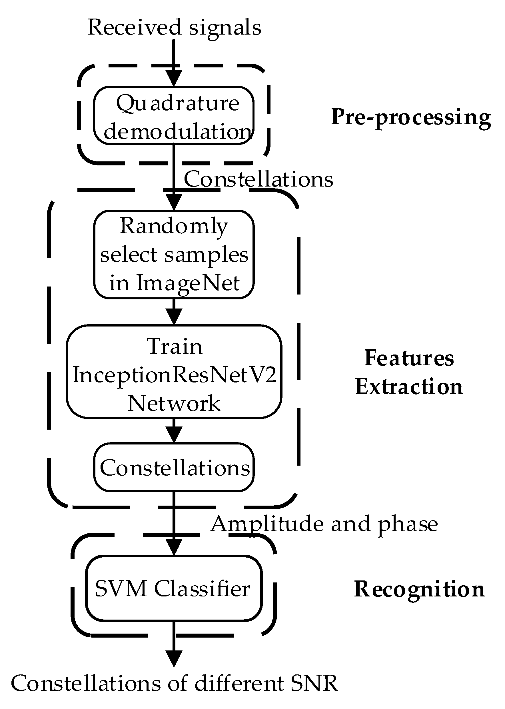
The proposed InceptionResnetV2-TA algorithm consists of three steps: pre-processing, features extraction and recognition. The block diagram of the InceptionResnetV2-TA algorithm is shown in Figure 1. In the pre-processing operation, the signal constellation is obtained by orthogonally demodulating the signal to be detected. In the feature extraction operation, the idea of transfer adaptation is used to randomly select 12 types of image samples from the ImageNet dataset and send them to the InceptionResNetV2 network to complete the training. Then the training weights are saved, and finally, the constellation map is sent to the network that stores the weights for further training, which are used to get the effective features in the constellation. In the recognition operation, the effective features learned by the network are sent to the classifier, and the recognition of the modulation mode of the digital signal is completed. SVM is used to classify the features extracted from the constellation diagram of digital signals to the classifier, so as to achieve the correct recognition of the three signal modulation modes. Because of the particularity of the constellation chart data set used in this paper, it is different from the common image data set.
2.2. Preprocessing
The analog signal at the transmitting end is converted into a baseband signal through three processes of sampling, quantization and encoding, and then reaches the receiving end through a frequency band transmission. Because the signal carries noise during transmission, the signal obtained at the receiving end is a noisy signal, which is written as follows:
is the amplitude value of the m-th symbol, Ts is the symbol interval, ejθm is a constellation point, fc is the carrier frequency of the signal, θi is the carrier phase difference and g(t) is a rectangular pulse function. N is the number of symbols in the observation time T, and n(t) is noise.
In digital communication, the constellation diagram is the most direct way to observe the amplitude and phase of a signal. It is obtained by orthogonally demodulating the received signal. After receiving the signal s(t), the receiver divides the signal into two channels and multiplies them with two carriers with a phase difference of π/2, and then filters the high-frequency components through a low-pass filter. Finally, two relatively independent components are obtained: the in-phase (I) component and quadrature (Q) component. The two components are orthogonal to each other and are irrelevant. These two components are usually expressed in complex form as , corresponding to a point on the complex plane, which is called a constellation point. Moreover, each type of amplitude-phase modulation signal has a corresponding point set used to represent such a modulation method, and these point sets form a constellation diagram representing the signal. The modulus indicates the amplitude change of the signal, and the phase indicates the phase change of the signal. Finally, the constellation map is sent to the InceptionResNetV2 network to complete the feature extraction operation.
2.3. Transfer Learning
Transfer learning, as an important branch of machine learning, aims to use the similarity between data, tasks or models to transfer the knowledge learned from the source project to the target project. Compared with machine learning, the advantages of transfer learning are: in the data distribution, it can obey different distributions; in the data annotation, a large number of data annotations are not needed; in the model, the features and weights obtained from the training model can be used to train new models and complete new tasks [21,22,23].
Transfer learning is mainly divided into four categories: sample-based, feature-based, model-based and relationship-based ones [24,25,26]. In this paper, the InceptionResNetV2 network is combined with feature-based transfer learning; that is to say, the weight matrix can be shared from the ImageNet dataset and the constellation map to implement the fine tuning, and the transfer adaptation method is applied to the network.
Feature-based transfer adaptation methods are further divided into edge distribution adaptation and conditional distribution adaptation. In the edge distribution adaptation, in order to reduce the difference between the edge distributions and , the empirical maximum mean difference (MMD) is used to measure the adaptation degree of different probability distributions. Minimize the distance between and for adaptation. MMD is defined as follows:
is an infinite-order, nonlinear feature map in kernel space. According to Taylor’s theorem, can be expanded into an infinite-order polynomial series, so it has the ability to adapt to statistics of different orders with different probability distributions.
In the conditional distribution adaptation, minimizing the difference between the conditional distributions and is extremely important to the robustness of the distribution adaptation. Direct annotation learning is used to obtain the pre-labeling in the constellation diagram and then obtain conditional distribution distance. When the classifier is unknown, the class posterior probabilities and are difficult to fit. Then, the moments of the class conditional distribution and are matched. Using the pre-labeled dB values in the constellation map and the actual label in the ImageNet dataset, each class in the constellation map can be used to obtain class conditional distributions and . Among them, the distance between the metric conditional distributions and can be obtained by the extension of Equation (2):
is an image collection belonging to the category in the ImageNet dataset, and is the actual label of the image ; are a set of images whose dB values belong to the category in the constellation map, and y(xj) is the dB value of the constellation map xj. Combine Equations (2) and (3) to get the adapted regular term as follows:
By minimizing the regular term, any order moment estimation of these two distributions can be adapted in infinite order nonlinear feature maps. Now, given the labeled ImageNet dataset and unlabeled constellation , satisfy , , , . Because there are 12 types of images in the constellation diagram, 12 types of images are randomly selected in the ImageNet dataset and sent to the InceptionResNetV2 network to complete the training task. According to the transfer adaptation principle, the weight matrix obtained by training is applied to the constellation. InceptionResNetV2 network, while learning feature F or classification model f, minimizes the difference between the edge distributions and , and minimizes the difference between the conditional distribution and . Finally, the classifier can be accurately generalized into the constellation after training on the ImageNet dataset [27,28,29,30,31,32]. Compared to using the ImageNet dataset to train the network directly, this article selects the same number of images in the constellation map to complete the training task. The obtained weight matrix is then used to train the constellation map. Finally, the correct classification of the constellation map is used to improve the recognition accuracy of the digital signal modulation method.
3. InceptionResNetV2-TA Network
The InceptionResNetV2 network is from GoogLeNet. The traditional neural network structures all improve the training effect by increasing the network depth, but increasing the number of layers will cause overfitting, gradient disappearance, gradient explosion and so on. The solution is to change the full connection to a sparse connection, but the hardware optimizes the dense matrix, so the dense local matrix structure is calculated for the optimal local sparse structure to obtain the Inception structure. Inception uses the computing resources more efficiently, and can extract more features under the same calculation amount to improve the training result. Through the concatenate operation, feature maps with different kernel scales are aggregated to increase the network’s adaptability to the scale and the network width, and improve resource utilization. Since all the convolution kernels take the output of the previous layer as input, and the calculation of the 5 × 5 convolution kernel is too large, the output of the previous layer is combined to the network in network (NIN) method.
The Inception module uses a 1 × 1 convolution for two purposes: one is to superimpose more convolutions on the receptive fields of the same size to extract richer features in the constellation map; the other is to reduce the dimensions and the computational complexity. The 1 × 1 convolution in the network before the 3 × 3 and 5 × 5 convolutions is used for dimensionality reduction. Secondly, the aggregation operation is performed on convolutions of multiple sizes. It is calculated by decomposing a sparse matrix into a dense matrix to improve the convergence speed.
In a traditional convolution layer, the input is convolved with a convolution kernel of one scale (such as 3 × 3), the output data is a fixed dimension (such as 256 features), and the features are evenly distributed on the 3 × 3 scale. The Inception module extracts the effective features in the constellation map on multiple different scales, which are no longer evenly distributed. Instead, the features with high correlation are grouped together, and the features with low or irrelevance are weakened, making the output feature redundancy relatively small and the convergence speed faster. Besides the Inception module, the fully connected layer was replaced by global average pooling to reduce parameters. At the same time, the network also adds a batch normalization (BN) layer. When the BN layer acts on a layer of the neural network, it can normalize each mini-batch constellation map to avoid gradient disappearance [33].
is the training set of any given constellation, and is the set of constellations. In the back-propagation algorithm, we also need to calculate Jacobians:
For any dimension input , after normalization, it can be written as follows:
This normalization operation can speed up training. For any activation value , and parameters , , the normalized values after translation and scaling are written as follows:
During training, the gradient of loss ℓ can be obtained through the back-propagated chain rule:
Stochastic gradient descent (SGD) is used in the network to optimize the network parameter and minimize the loss . When the input distribution of each layer changes (that is, covariate shift), gradient disappearance can be solved by the BN layer.
and are arbitrary transformations, and the loss is minimized by learning the network parameters and . At the same time, two 3 × 3 convolution kernels are used instead of 5 × 5 convolution kernels, and three 3 × 3 convolution kernels are used instead of 7 × 7 convolution kernels. Because it is more difficult to locally process high-dimensional features, and aggregation operations in low-dimensional space will not reduce the model’s ability to express, the n × n convolution kernel is decomposed into 1 × n and n × 1 convolution kernel.
This asymmetric convolution can obtain richer spatial features, improving feature diversity and model expression ability. At the same time, the number of parameters can be reduced, the calculation speed can be improved and overfitting can be reduced. For any one constellation, the probability that belongs to a different SNR is calculated by Equation (16):
is the training sample,
is an arbitrary label and is the logarithm. The cross-entropy loss function is written as follows:
Among them, represents the probability distribution of the true dB value; is the probability distribution of the dB value predicted by the trained model; and the cross-entropy loss function can measure the similarity between the two distributions. The lower the cross-entropy value, the closer the predicted distribution will be to the true distribution.
In addition, the network adds a residual structure on the original basis; that is, directly connected channels are added to the network, allowing the original input information in the constellation diagram to be directly transmitted to the subsequent layers, thereby speeding up training, preventing gradient dispersion, reducing network complexity and ensuring network depth while not degrading performance [34]. ReLU is used as the activation function, and the last layer of the model is connected to SVM to replace softmax.
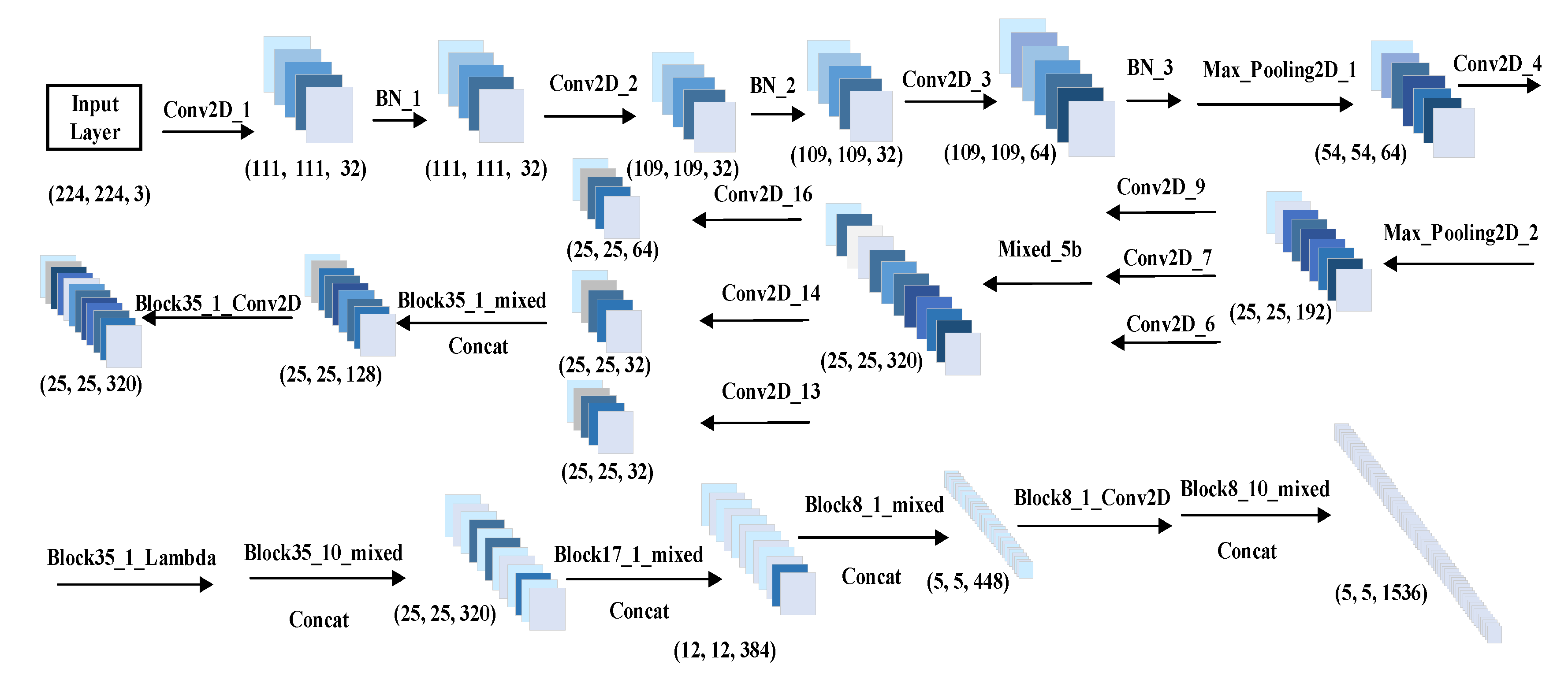
The idea of a kernel function is used to map the non-linear samples to high-dimensional space to be linearly separable, and then to maximize the classification interval between symbols in the constellation diagram to determine the optimal segmentation hyperplane. Unsupervised learning is used to extract the high-level features of the constellation map, which is input the SVM model to achieve the best classification accuracy and improve the recognition accuracy of digital signal modulation methods. InceptionResNetV2-TA network architecture is shown in Figure 2.
4. Experimental Results and Analysis
4.1. Recognition Performance Comparison
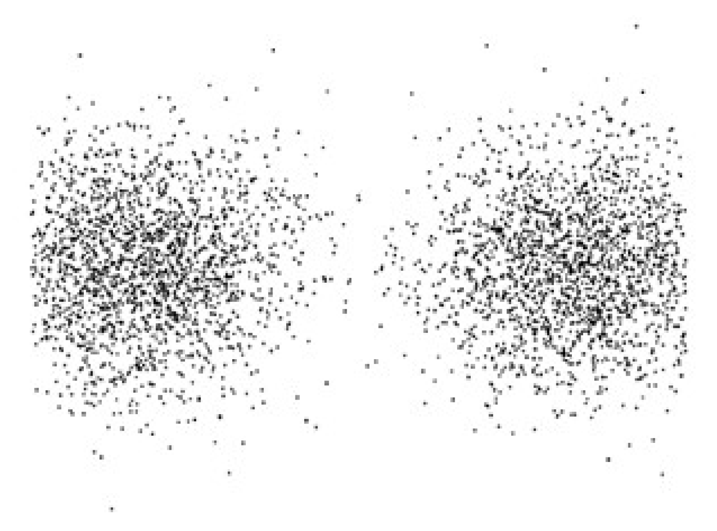
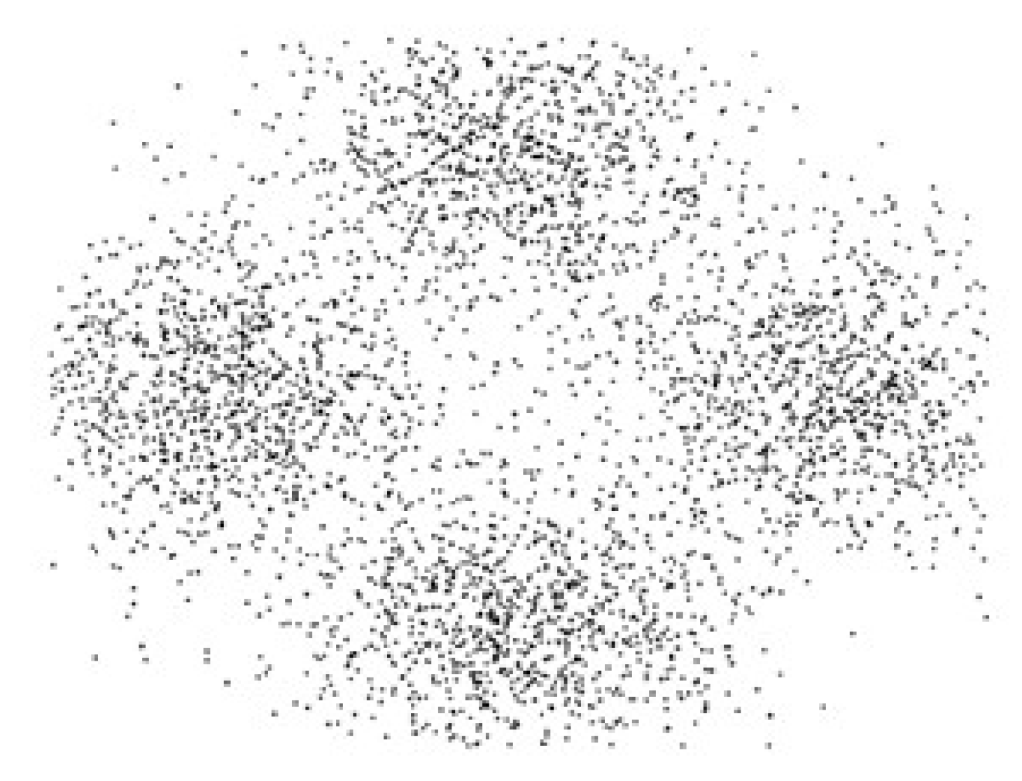
In order to verify the effectiveness of the algorithm, this paper uses Matlab to simulate phase-shift keying signals in digital communication systems to obtain the constellation diagrams of BPSK, QPSK and 8PSK at six low SNRs, which range from 1 to 12 dB. Figure 3, Figure 4 and Figure 5 are the constellation diagrams of the three signals when the SNR is 6 dB. The symbol rate of each signal is 1200 Bd, the number of symbols is 4000, the carrier frequency is 4800 Hz and the sampling frequency is 16 × 4800 Hz. Gaussian white noise is added to simulate the transmission of three signals on the Gaussian channel. At the same time, a Tensorflow-1.8.0+Keras-2.2.4 framework was built to train the InceptionResNetV2-TA network. The data set required for the experiments includes a training set and a test set. There are 9000 constellation maps in the training dataset and 2250 constellation maps in the test dataset. By training the network, it is able to classify the constellation diagrams of the three signals at low SNR, so as to correctly identify the digital signal modulation method.
In this paper, the InceptionResNetV2-TA algorithm is used to identify the modulation method of digital signals. At the same time, InceptionResNetV2, InceptionV3, ResNet50 and quasi hybrid likelihood ratio test-upper bound (QHLRT-UB) [35] are selected as comparison methods. The evaluation indicators required for the experiments are the recognition rates of the constellation diagrams of the three signals at low SNR; the five algorithms correspond to the overall recognition accuracy of the three data sets. The experimental results are shown in the figures below.
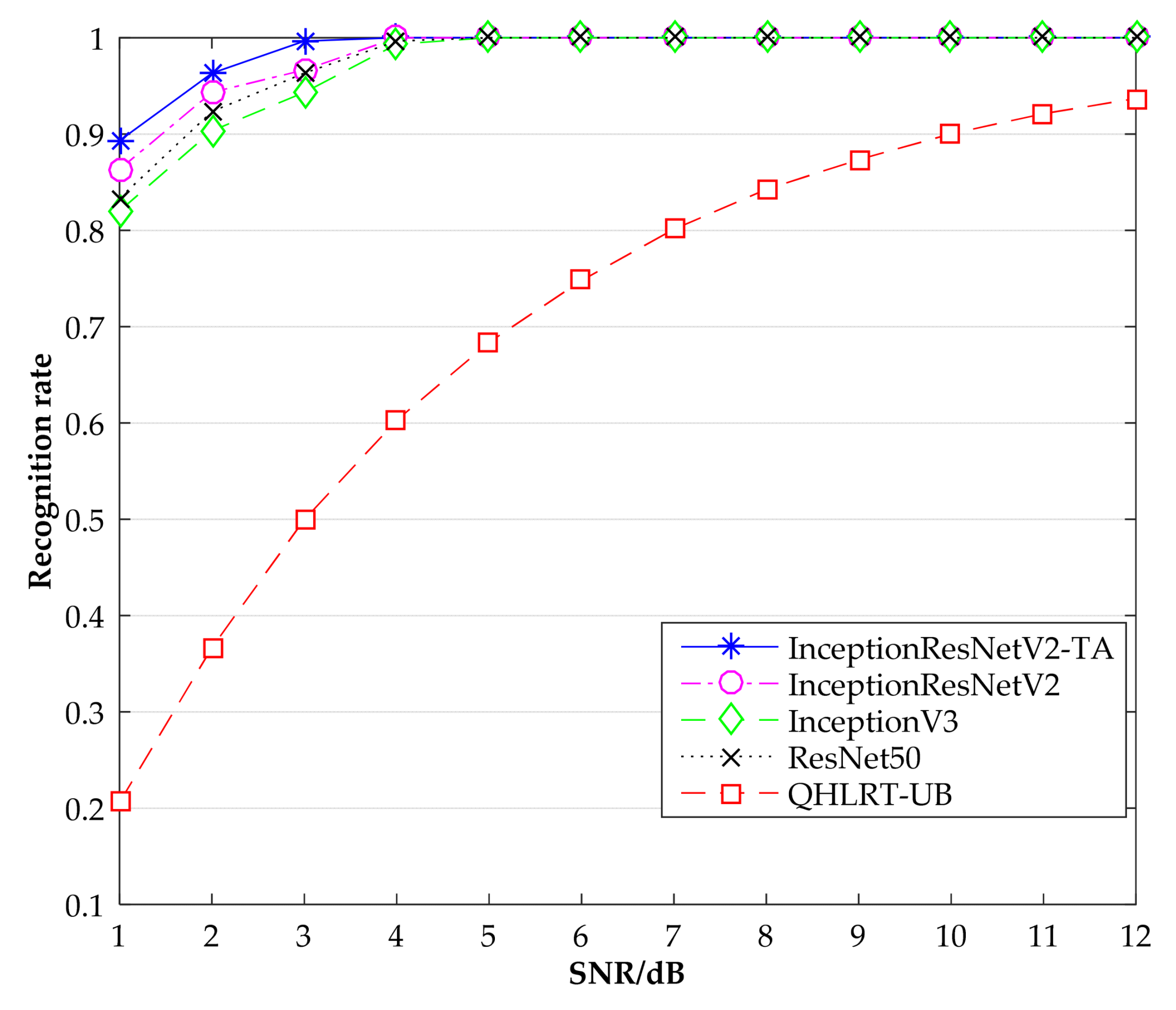
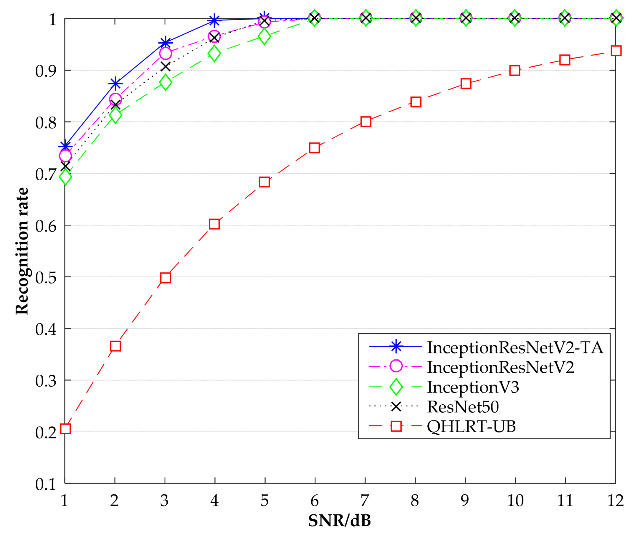
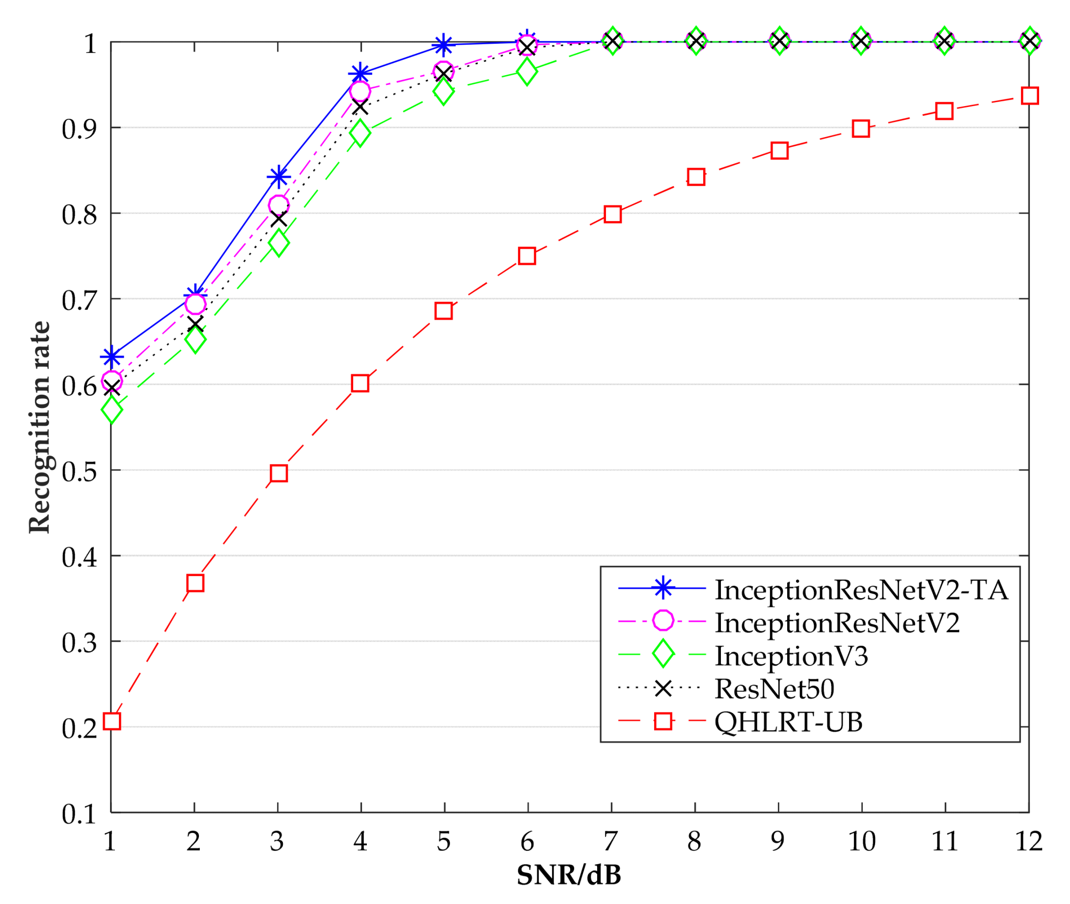
Figure 6, Figure 7 and Figure 8 show the recognition rates of the constellation diagrams of the three signals, BPSK, QPSK and 8PSK, at different SNRs. It can be seen from the figures that the recognition rate of each signal becomes larger as SNR increases. The algorithm proposed in this paper is significantly higher in recognition rate than the other three comparison algorithms.
Table 1 shows the specific results of the recognition rates of the three signals obtained by the five algorithms, including InceptionResNetV2-TA, InceptionResNetV2, InceptionV3, ResNet50 and QHLRT-UB. It can be seen that the InceptionResNetV2-TA algorithm has the highest recognition rate of the constellation diagrams of the three signals, followed by the InceptionResNetV2 algorithm. In Table 1, when SNR is 3 dB, the recognition rate of BPSK reaches 99.66%, which is 3% higher than the InceptionResNetV2 algorithm. When SNR is 4 dB, the recognition rate of QPSK reaches 99.66%. Compared with the InceptionResNetV2 algorithm, the recognition rate is improved by 3%. When SNR is 5 dB, the recognition rate of 8PSK reaches 99.66%, which is 3.33% higher than that of InceptionResNetV2 algorithm. When SNR was greater than 7 dB, the recognition rate of the four neural networks for the three signals reached 100%, while the recognition rate of QHLRT-UB algorithm was only about 80%. This shows that the recognition rate of digital signal modulation by neural network is higher than that by classical algorithm.
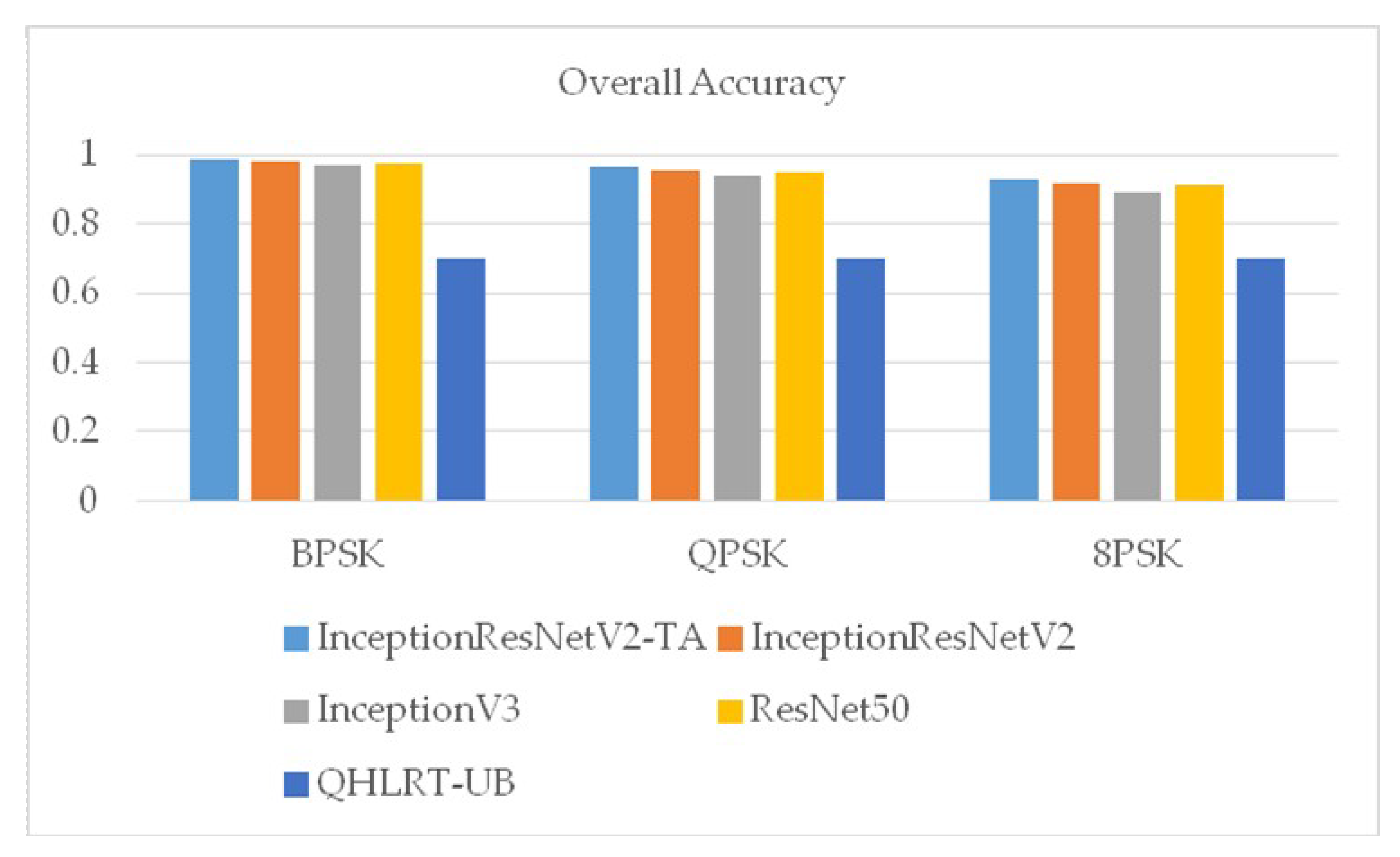
Figure 9 shows the overall recognition rates of the three signals of BPSK, QPSK and 8PSK by the five algorithms. It can be seen from the figure that the overall recognition rates of the three signals by InceptionResNetV2-TA algorithm proposed in this paper were the highest.
When SNR is higher than 4 dB, the recognition rate of the four algorithms for BPSK reaches the highest and remains stable, and the recognition rate is always 100%.When SNR is higher than 5 dB, the recognition rate of the four algorithms for QPSK reaches 100%.When SNR is higher than 6 dB, the recognition rate of the four algorithms for 8PSK is 100%.This indicates that as SNR gets higher and higher, the recognition accuracy of various algorithms for three digital signal modulation modes will gradually increase and remain stable under a certain SNR.
4.2. Analysis of Computational Complexity
The proposed algorithm of the paper and the comparison algorithms are based on convolutional neural networks. The complexity of a convolutional neural network is divided into time complexity and space complexity. The time complexity includes the number of convolutional layers and channels in the network (i.e., the number of convolutional kernels), and the overall time complexity is the sum of the time complexity of all convolutional layers. The space complexity includes the total number of parameters and the characteristic graph of each layer.
The number of parameters refers to the weighted parameters of all convolutional layers with parameters (i.e., the volume of the network model), and the characteristic graph refers to the size of the output characteristic graph calculated by each layer during the real-time operation of the network. The total number of parameters is only related to the size of the convolution kernel, the number of channels and the number of layers, not to the size of the input data. The output characteristic graph is the multiplication of the space size and the number of channels. The time complexity determines the training time and testing time of the model. If the complexity is too high, the training and prediction of the model will cost a lot of time, and fast prediction cannot be achieved.
The space complexity determines the number of parameters of the network model. The more parameters in the network, the more data required for training, which will easily lead to the model overfitting. The spatial complexity of the full connection layer is closely related to the size of the input image. The larger the size of the input image, the larger the size of the model. The parameters of the full connection layer will become larger and larger, and the complexity of the network will increase. In the inceptionresnetv2-ta network, the time complexity is reduced by using 1 × 1 convolution to reduce dimension. In addition, 3 × 3 convolution is used instead of 5 × 5 convolution, which can effectively reduce the complexity of time and space, and use these complexities to improve the depth and width of the model, so that the network model has a larger capacity.
Compared the classical methods, the complexity of InceptionResNetV2-TA algorithm depends on the transfer adaptation part. In most cases, the constellation diagram of digital signals is directly classified when it is identified. The constellation map is sent to the neural network and the amplitude and phase features are extracted, and then the features are sent to the classifier to complete the classification task. In this paper, the method of transfer adaptation is adopted. Before constellation images are sent to the neural network, the number of images to be recognized is first determined, and then images with the same number of categories are selected from ImageNet and sent to the neural network for pre-training. The weights of the trained network will be optimized, and then the optimized network will be used to classify the constellation diagram. Finally, the accuracy of this network is higher than that of the neural network without transfer adaptation. It should also be noted that the number of categories of images selected in ImageNet must be the same as that of the constellation to be recognized; otherwise, the recognition rate will be reduced. Compared with the complexity of the classical algorithm, the algorithm proposed in this paper is better. Additionally, the recognition accuracy of digital signal modulation can be comparable to that of classical algorithms.
5. Conclusions
This paper proposed the InceptionResNetV2-TA algorithm, which improves the recognition accuracy of digital signal modulation by combining transferring adaptation with InceptionResNetV2. Experiments showed that the algorithm has good recognition performance in the recognition of the modulation method of the phase shift keying signal. Especially at different SNRs, the recognition rate of the three signal modulation modes of BPSK, QPSK and 8PSK is higher than in the other three comparison algorithms. Future work will focus on identifying more types of digital signals at low SNRs.
Author Contributions
This article was completed by all authors. K.J. and A.W. designed and implemented the classification algorithm. J.Z. did an experimental analysis of the algorithm. H.W. and Y.I. participated in the writing of the paper. All authors have read and agreed to the published version of the manuscript.
Funding
This research was funded by National Natural Science Foundation of China (NSFC-61671190).
Acknowledgments
The authors would like to thank the support of the laboratory and university.
Conflicts of Interest
The authors declare no conflict of interest.
References
- Weaver, C.S.; Cole, C.A.; Krumland, R.B. The Automatic Classification of Modulation Types by Pattern Recognition; Technical Report No.1829-2; Stanford Electronics Laboratories, Stanford University: Stanford, CA, USA, 1969. [Google Scholar]
- Yang, J.; Wang, X.; Cheng, N. Research on Signal Modulation Recognition Algorithm Based on Feature Parameter Extraction. Comput. Eng. Softw. 2018, 39, 180–184. [Google Scholar]
- Shi, Q.; Gong, Y.; Guan, Y. Modulation Classification for Asynchronous High-Order QAM Signals. Wirel. Commun. Mob. Comput. 2011, 11, 1415–1422. [Google Scholar] [CrossRef]
- Dobre, O.A.; Abdi, A.; Bar-Ness, Y.; Su, W. Survey of Automatic Modulation Classification Techniques: Classical Approaches and New Trends. Commun. IET 2007, 1, 137–156. [Google Scholar] [CrossRef] [Green Version]
- Li, J.; Feng, X. Modulation classification algorithm based on support vector machines and cyclic cumulants. Syst. Eng. Electron. Technol. 2007, 29, 520–523. [Google Scholar]
- Feng, X.; Yuan, H. Hierarchical Modulation Classification Algorithm Based on Higher-order Cyclic Cumulants and Support Vector Machines. Telecommun. Eng. 2012, 52, 878–882. [Google Scholar]
- Feng, X.; Luo, F.; Yang, J.; Hu, Z. Automatic Modulation Recognition Using Support Vector Machines Based on Wavelet Transform. J. Electron. Meas. Instrum. 2009, 23, 87–92. [Google Scholar]
- Li, Y.; Ge, J.; Lin, Y. Modulation Recognition Using Entropy Features and SVM. Syst. Eng. Electron. 2012, 34, 1691–1695. [Google Scholar]
- Tan, Z.; Shi, J.; Hu, J. Low-Order Digital Modulation Recognition Algorithm based on Random Forest. Commun. Technol. 2018, 51, 527–532. [Google Scholar]
- Gao, Y.; Chen, T. Cognitive Radio Signal Modulation Recognition based on Decision Tree. Commun. Technol. 2019, 52, 1563–1568. [Google Scholar]
- Zhang, J.; Wang, B.; Wang, Y.; Liu, M. An Algorithm for Recognition and Parameters Estimation of OFDM in Alpha Stable Distribution Noise. Acta Electron. Sin. 2018, 46, 1391–1396. [Google Scholar]
- Niu, G.; Yao, X.; Yan, Y.; Wang, C. Modulation Recognition Algorithm of Digital and Analog Mixed Signal Based on Work. Comput. Eng. 2016, 42, 101–104. [Google Scholar]
- Huang, Y.; Jia, Z.; Zhou, X.; Lu, J. Demodulation with Deep Learning. Telecommun. Eng. 2017, 57, 741–744. [Google Scholar]
- Hou, T.; Zheng, Y. Communication Signal Modulation Recognition Based on Deep Learning. Radio Eng. 2019, 49, 796–800. [Google Scholar]
- Peng, S.; Jiang, H.; Wang, H. Modulation Classification Based on Signal Constellation Diagrams and Deep Learning. IEEE Trans. Neural Netw. Learn. Syst. 2019, 30, 718–727. [Google Scholar] [CrossRef] [PubMed]
- Wang, Y.; Liu, M.; Yang, J.; Guan, G. Data-Driven Deep Learning for Automatic Modulation Recognition in Cognitive Radios. IEEE Trans. Veh. Technol. 2019, 68, 4074–4077. [Google Scholar] [CrossRef]
- Peng, C.; Diao, W.; Du, Z. Digital Modulation Recognition Based on Deep Convolutional Neural Network. Comput. Meas. Control 2018, 26, 222–226. [Google Scholar]
- Yang, F.; Yang, L.; Wang, D.; Qi, P.; Wang, H. Method of Modulation Recognition Based on Combination Algorithm of K-means Clustering and Grading Training SVM. IEEE Trans. China Commun. 2018, 15, 55–63. [Google Scholar]
- Li, Z.; Yang, F.; Li, H.; Huang, H.; Pan, Z. Method of Neural Network Modulation Recognition Based on Clustering and Polak-Ribiere Algorithm. IEEE Trans. J. Syst. Eng. Electron. 2014, 25, 742–747. [Google Scholar]
- Cui, X.; Xiong, G. Digital Modulation Recognition based on Constellation Diagram Fuzzy Analysis. Commun. Technol. 2016, 49, 1155–1158. [Google Scholar]
- Hsiao, P.; Chang, F.; Lin, Y. Learning Discriminatively Reconstructed Source Data for Object Recognition with Few Examples. IEEE Trans. Image Process. 2016, 25, 3518–3532. [Google Scholar] [CrossRef]
- Shao, L.; Zhu, F.; Li, X. Transfer Learning for Visual Categorization: A Survey. IEEE Trans. Neural Netw. Learn. Syst. 2015, 26, 1019–1034. [Google Scholar] [CrossRef]
- Yang, L.; Jing, L.; Yu, J.; Ng, M.K. Learning Transferred Weights From Co-Occurrence Data for Heterogeneous Transfer Learning. IEEE Trans. Neural Netw. Learn. Syst. 2016, 27, 2187–2200. [Google Scholar] [CrossRef] [PubMed]
- Long, M.; Wang, J.; Cao, Y.; Sun, J.; Yu, P.S. Deep Learning of Transferable Representation for Scalable Domain Adaptation. IEEE Trans. Knowl. Data Eng. 2016, 28, 2027–2040. [Google Scholar] [CrossRef]
- Shao, K.; Zhu, Y.; Zhao, D. StarCraft Micromanagement with Reinforcement Learning and Curriculum Transfer Learning. IEEE Trans. Emerg. Top. Comput. Intell. 2019, 3, 73–84. [Google Scholar] [CrossRef] [Green Version]
- Long, M.; Wang, J.; Sun, J.; Yu, P.S. Domain invariant transfer kernel learning. IEEE Trans. Knowl. Data Eng. 2015, 27, 1519–1532. [Google Scholar] [CrossRef]
- Pan, S.J.; Tsang, I.W.; Kwok, J.T.; Yang, Q. Domain adaptation via transfer component analysis. IEEE Trans. Neural Netw. 2011, 22, 199–210. [Google Scholar] [CrossRef] [Green Version]
- Si, S.; Tao, D.; Geng, B. Bregman divergence-based regularization for transfer subspace learning. IEEE Trans. Knowl. Data Eng. 2010, 22, 929–942. [Google Scholar] [CrossRef]
- Chalmers, E.; Contreras, E.B.; Robertson, B.; Luczak, A.; Gruber, A. Learning to Predict Consequences as a Method of Knowledge Transfer in Reinforcement Learning. IEEE Trans. Neural Netw. Learn. Syst. 2018, 29, 2259–2270. [Google Scholar] [CrossRef]
- Ding, Z.; Shao, M.; Fu, Y. Incomplete Multisource Transfer Learning. IEEE Trans. Neural Netw. Learn. Syst. 2018, 29, 310–323. [Google Scholar] [CrossRef]
- Ding, Z.; Fu, Y. Deep Transfer Low-Rank Coding for Cross-Domain Learning. IEEE Trans. Neural Netw. Learn. Syst. 2019, 30, 1768–1779. [Google Scholar] [CrossRef]
- Wang, J.; Zhao, P.; Hoi, S.C.H.; Jin, R. Online feature selection and its applications. IEEE Trans. Knowl. Data Eng. 2014, 26, 698–710. [Google Scholar] [CrossRef] [Green Version]
- Ioffe, S.; Szegedy, C. Batch normalization: Accelerating deep network training by reducing internal covariate shift. In Proceedings of the 32nd International Conference on Machine Learning, Lille, France, 7–9 July 2015; Volume 37, pp. 448–456. [Google Scholar]
- He, K.; Zhang, X.; Ren, S.; Sun, J. Deep Residual Learning for Image Recognition. IEEE Trans. CVPR 2016, 1, 770–778. [Google Scholar]
- Hameed, F.; Dobre, O.; Popescu, D. On the likelihood-based approach to modulation classification. IEEE Trans. Wirel. Commun. 2009, 8, 5884–5892. [Google Scholar] [CrossRef]
Figure 1.
The block diagram of InceptionResnetV2-TA Algorithm.

Figure 2.
InceptionResNetV2-TA network architecture.

Figure 3.
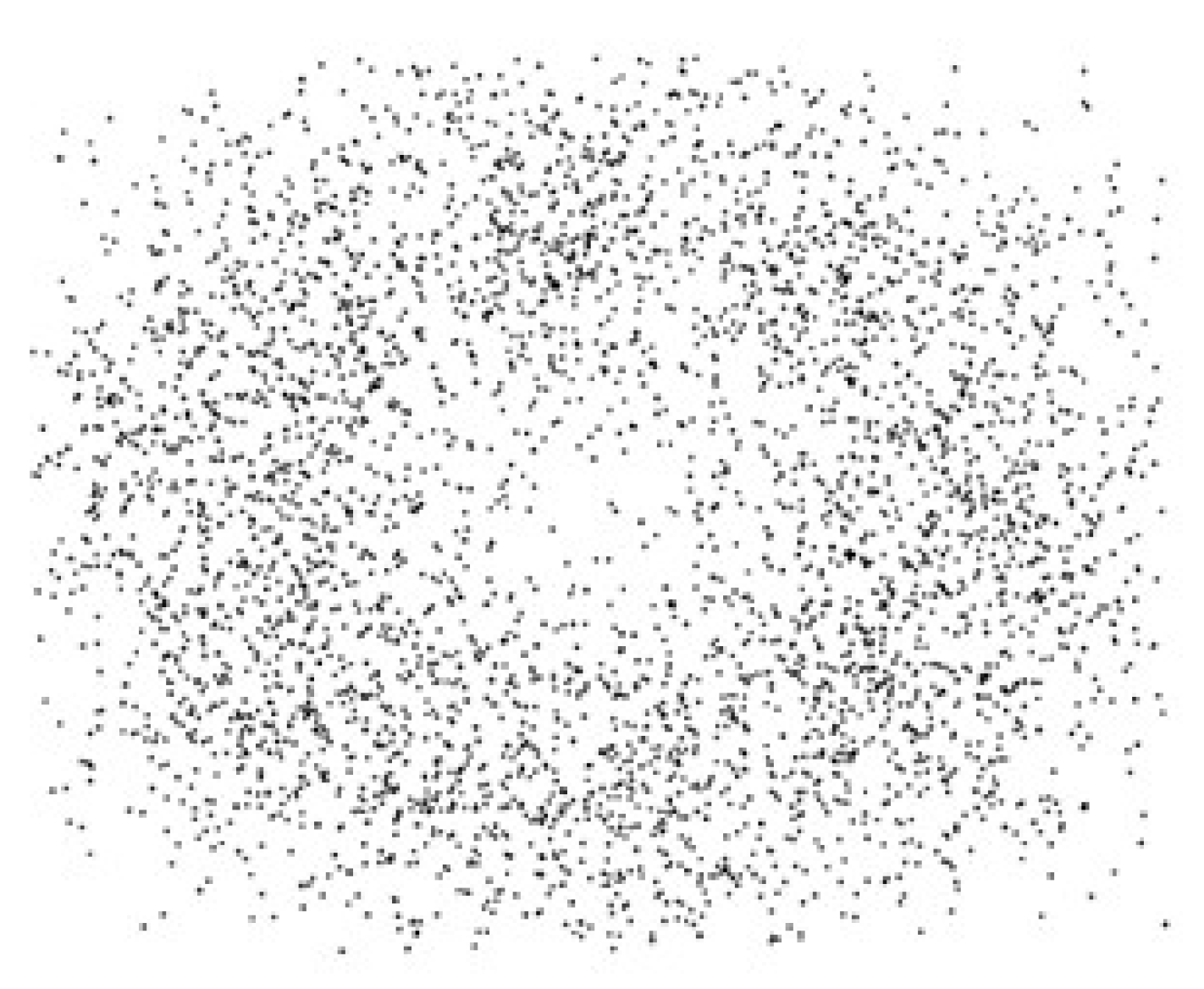
BPSK (SNR = 6 dB).

Figure 4.
QPSK (SNR = 6 dB).

Figure 5.
8PSK (SNR = 6 dB).

Figure 6.
Recognition rate comparison of BPSK by different methods.

Figure 7.
Recognition rate comparison of QPSK by different methods.

Figure 8.
Recognition rate comparison of 8PSK by different methods.

Figure 9.
Overall recognition rates for the three signals.


Table 1.
Recognition rate comparison of BPSK, QPSK and 8PSK at different SNRs.
| Recognition Rate | InceptionResNetV2-TA | InceptionResNetV2 | Inceptio-nV3 | ResNet50 | QHLRT-UB | |
|---|---|---|---|---|---|---|
| BPSK | 1 dB | 0.8933 | 0.8633 | 0.82 | 0.8333 | 2060 |
| 2 dB | 0.9633 | 0.9433 | 0.9033 | 0.9233 | 0.3667 | |
| 3 dB | 0.9966 | 0.9666 | 0.9433 | 0.9633 | 0.4997 | |
| 4 dB | 1 | 1 | 0.9933 | 0.9966 | 0.6027 | |
| 5 dB | 1 | 1 | 1 | 1 | 0.6838 | |
| 6 dB | 1 | 1 | 1 | 1 | 0.748 | |
| 7 dB | 1 | 1 | 1 | 1 | 0.8012 | |
| 8 dB | 1 | 1 | 1 | 1 | 0.8425 | |
| 9 dB | 1 | 1 | 1 | 1 | 0.8735 | |
| 10 dB | 1 | 1 | 1 | 1 | 0.9003 | |
| 11 dB | 1 | 1 | 1 | 1 | 0.9212 | |
| 12 dB | 1 | 1 | 1 | 1 | 0.9369 | |
| QPSK | 1 dB | 0.7533 | 0.7333 | 0.6933 | 0.7133 | 0.2055 |
| 2 dB | 0.8733 | 0.8433 | 0.8133 | 0.8333 | 0.3658 | |
| 3 dB | 0.9533 | 0.9333 | 0.8766 | 0.9066 | 4989 | |
| 4 dB | 0.9966 | 0.9666 | 0.9333 | 0.9633 | 0.6033 | |
| 5 dB | 1 | 0.9933 | 0.9666 | 0.9966 | 0.6834 | |
| 6 dB | 1 | 1 | 1 | 1 | 0.7506 | |
| 7 dB | 1 | 1 | 1 | 1 | 0.8011 | |
| 8 dB | 1 | 1 | 1 | 1 | 0.8396 | |
| 9 dB | 1 | 1 | 1 | 1 | 0.8736 | |
| 10 dB | 1 | 1 | 1 | 1 | 0.9 | |
| 11 dB | 1 | 1 | 1 | 1 | 0.9206 | |
| 12 dB | 1 | 1 | 1 | 1 | 0.9367 | |
| 8PSK | 1 dB | 0.6333 | 0.6033 | 0.57 | 0.5966 | 0.2055 |
| 2 dB | 0.7033 | 0.6933 | 0.6533 | 0.67 | 0.3691 | |
| 3 dB | 0.8433 | 0.81 | 0.7666 | 0.7933 | 0.4971 | |
| 4 dB | 0.9633 | 0.9433 | 0.8933 | 0.9233 | 0.6019 | |
| 5 dB | 0.9966 | 0.9633 | 0.9433 | 0.9633 | 0.6864 | |
| 6 dB | 1 | 0.9966 | 0.9666 | 0.9933 | 0.7503 | |
| 7 dB | 1 | 1 | 1 | 1 | 0.799 | |
| 8 dB | 1 | 1 | 1 | 1 | 0.8416 | |
| 9 dB | 1 | 1 | 1 | 1 | 0.8743 | |
| 10 dB | 1 | 1 | 1 | 1 | 0.8988 | |
| 11 dB | 1 | 1 | 1 | 1 | 0.9203 | |
| 12 dB | 1 | 1 | 1 | 1 | 0.937 | |
© 2020 by the authors. Licensee MDPI, Basel, Switzerland. This article is an open access article distributed under the terms and conditions of the Creative Commons Attribution (CC BY) license (http://creativecommons.org/licenses/by/4.0/).
Share and Cite
MDPI and ACS Style
Jiang, K.; Zhang, J.; Wu, H.; Wang, A.; Iwahori, Y. A Novel Digital Modulation Recognition Algorithm Based on Deep Convolutional Neural Network. Appl. Sci. 2020, 10, 1166. https://0-doi-org.brum.beds.ac.uk/10.3390/app10031166
AMA Style
Jiang K, Zhang J, Wu H, Wang A, Iwahori Y. A Novel Digital Modulation Recognition Algorithm Based on Deep Convolutional Neural Network. Applied Sciences. 2020; 10(3):1166. https://0-doi-org.brum.beds.ac.uk/10.3390/app10031166
Chicago/Turabian StyleJiang, Kaiyuan, Jiawei Zhang, Haibin Wu, Aili Wang, and Yuji Iwahori. 2020. "A Novel Digital Modulation Recognition Algorithm Based on Deep Convolutional Neural Network" Applied Sciences 10, no. 3: 1166. https://0-doi-org.brum.beds.ac.uk/10.3390/app10031166
Note that from the first issue of 2016, this journal uses article numbers instead of page numbers. See further details here.