1. Introduction
Tomato (
Lycopersicon esculentum) occupies a prominent place in the Mexican agricultural economy. In fact, Mexico is the world’s leading supplier of tomatoes, with an international market share of 25.11% of the value of world exports [
1]. According to the
Servicio de Información Agroalimentaria y Pesquera (SIAP), it is estimated that tomato exports will grow up to 3.84 million tons in 2024.
Healthy plants need to be protected from diseases to guarantee the quality and quantity of crop since they are highly affected by diseases which cause dramatic losses in agricultural economy [
2,
3].
It is important to mention that providing early monitoring is essential for choosing the correct treatment and stopping the disease from spreading [
4]. Commonly, the detection and identification of diseases is achieved by experts by simple observation [
4]. However, this task needs continuous monitoring by experts [
5] since it can be erroneously diagnosed by farmers because they usually judge the symptoms by their experience; thus, a precise recognition technology is essential for this task.
Deep Learning (DL) is taking major advances in solving problems because the adaptability of computer vision techniques tan can be adapted, and its results outperform the state-of-the-art in several topics [
6]. According to Ferentinos [
7], DL refers to the use of artificial neural networks (ANNs) architectures that contain a quite large number of processing layers, as opposed to “shallower” architectures of more traditional ANN methodologies. The main advantage of DL is the ability to exploit directly raw data without using hand-crafted features [
3].
In DL, Convolutional Neural Networks (CNNs) are a class of deep ANN, and they have many applications, including complex tasks, such as image classification and object recognition, which lead to a significant improvement in image classification in several topics, such as agriculture. Motivated by the DL breakthrough and the rapid development of CNNs, many powerful architectures have emerged, such as AlexNet [
8], GoogleNet [
9], Inception V3 [
10], Residual Network (ResNet) 50, and ResNet 18 [
11].
In this work, the architectures previously mentioned are used to classify tomato diseases, in order to develop a comparison between these CNN architectures performance, supporting in the selection of an automatic system that allows the extension of its the applications in the field of agriculture. The main contribution of this paper focuses on a detailed description of the operation of each ANN, in addition to its implementation to be applied in a database composed of a series of images related to diseased tomato plants and, in this way, to be able to objectively know through a direct comparison the behavior of the different ANNs for future applications. On the other hand, with the aim of determining which is the architecture that best models the problem and achieves a good classification of tomato plant diseases and validating it through different statistical metrics, the CNN models can be implemented in this way as an automated system designed to identify plant diseases, which could be of great help to technicians and experts in agriculture.
The rest of this paper is organized as follows:
Section 2 presents an overview of related work.
Section 3 introduces the five state-of-the-art CNN architectures and the experiments.
Section 4 shows the results.
Section 5 holds the discussion and, finally,
Section 6 reports the final conclusions.
2. Related Work
In recent years, the research of agricultural plant disease classification has been a relevant topic. Developing a reliable system that is applicable for a large number of classes is a very challenging task. Due to this, several studies have been using CNNs for classification and detection of diseases. In the case of Kawasaki et al. [
12], it is proposed the use of CNNs to distinguish healthy cucumbers from unhealthy by using images of leaves. The authors introduced a CNN architecture, which uses the Caffe framework [
13], including convolutional layers, pooling layers, and local contrast normalization layers. They achieved an accuracy of 94.9% under the 4-fold cross-validation strategy.
Another approach for cucumber leaf diseases classification is that proposed by Fujita et al. [
14], which presents a CNN composed by four convolutional layers, pooling, and local response normalization (LRN) operations. The parameters of the LRN were the same parameters from AlexNet architecture. At last, their classification system attained an average of 82.3% accuracy under the 4-fold cross validation strategy.
Sladojevic et al. [
15] developed a plant disease recognition model, based on leaf image classification, by the use of CNNs. Their developed model is able to recognize 13 different types of plant diseases. In addition, they use Caffe as the DL framework. The experimental results showed a precision between 91% and 98%, and the final overall accuracy of the trained model was 96.3%.
On the other hand, Mohanty et al. [
16] evaluated well-known architectures of CNNs, AlexNet and GoogleNet, to identify 14 crops species and 26 diseases by using the PlantVillage dataset [
17]. They used different training-test distributions to measure the CNN performance: 80–20, 60–40, 50–50, 40–60, and 20–80%. Finally, the performance of their models was based on the ability to predict the correct crop diseases pair. The best performing model achieves a mean F1 score of 0.9934 (overall accuracy of 99.35%).
Moreover, Nachtigall et al. [
18] made use of CNNs to detect and classify nutritional deficiencies and damage on apple trees. AlexNet was used as CNN architecture, so they made a comparison between Multilayer Perceptron (MLP) and the CNN, which was compared with seven volunteer experts. The results showed an accuracy of 97.3% obtained by CNN, while the human experts had 96%, and the MLP obtained the lowest accuracy at 77.3%.
Furthermore, Brahimi et al. [
3] introduced CNN as a learning algorithm for classifying tomato diseases. They used the standard architectures, AlexNet and GoogleNet, and they concluded that DL outperforms other classification techniques (e.g., Random Forest, Support Vector Machine). For comparison purposes, they computed accuracy, macro precision, macro recall, and macro F-score. They obtained results reaching 99.18% accuracy.
DeChant et al. [
19] applied a CNN architecture to classify northern leaf blight lesions on images of maize plants. From the total number of images, 70% were used for training, 15% for validation, and 15% for testing. Their proposed system achieved 96.7% accuracy on test set images not used in training. Additionally, Lu et al. [
20] presented a novel rice diseases identification method based on CNNs techniques; the architecture used to identify 10 common rice diseases was AlexNet, and finally, the model achieved an accuracy of 95.48% under 10-fold cross validation.
In addition, Brahimi et al. [
6] tested multiple state-of-the-art CNN (AlexNet, DenseNet 169 [
21], Inception V3, ResNet 34 [
11], SqueezeNet 1.1 [
22], and Visual Geometry Group (VGG) 13 [
23]) for plant diseases classification using three different strategies. Two of these are based on transfer learning, and the last one was based on shallow strategy. The dataset was divided into 80% for training and 20% for evaluation. The final model accuracy reached was 99.76%, and they concluded that the most successful learning strategy was transfer learning. It is important to note that one of the main differences between this work and the one proposed here are the ANNs implemented for comparison since, based on the results of this work, the selection of an ANN was limited to only three of those that were used, including GoogleNet and other versions of ResNet, that presented significant results in the literature.
Moreover, Wang et al. [
24] proposed a DL approach to estimate disease severity. The best model was VGG 16 trained with transfer learning, which yields an overall accuracy of 90.4% on the hold-out test set. On the other hand, Wang et al. [
25] introduced a method for crop disease images classification by combining CNN and transfer learning. Their CNN with five convolutional layers reached 90.84% and demonstrated that the combination of CNN and transfer learning strategy is effective for classification of various crop diseases.
Rangarajan et al. [
26] used AlexNet and VGG 16 for classifying six different diseases and a healthy class of tomato. The performance was evaluated by modifying the number of images, setting different batch sizes, and varying the weight and bias learning rate. They concluded that AlexNet provides a better accuracy with the minimum execution time compared to VGG 16. It should be noted that, taking into account that this work is also aimed at the classification of diseases present in tomato plants, the development of the proposed methodology is based on the results reported by this comparison, allowing support in the delimitation of the work and selection of architectures to implement, while being able to discard the implementation of VGG 16 due to the disadvantages that it presents in comparison with AlexNet, especially in the computational cost.
Finally, Khandelwal and Raman [
27] detected plant diseases using different state-of-the-art approaches. In this work, their model was able to attain a high average accuracy of 99.374% using transfer learning.
Table 1 summarizes the studied approaches and methodologies that use DL models for plant diseases classification, where the results are based on accuracy, as well as the metrics that they used and the final results that are based on accuracy.
Based on these related works, it was decided to limit the inclusion of the ANN: AlexNet, GoogleNet, Inception V3, ResNEt 18, and ResNet 50, to carry out the comparison proposed in this work. These ANN were selected due to the significant behavior with which they have been reported, supported by their results.
3. Materials and Methods
This section describes the details of the CNNs implemented for plant disease classification of tomato plant leaves in this work. This study concentrates on finding the most appropriate pre-trained CNN model. The entire procedure is divided into 4 basic steps: data acquisition, data training, data classification, and data evaluation, which are detailed below.
3.1. Data Acquisition
The
PlantVillage - Dataset is an open repository that contains 54,323 images of 14 crops and 38 kinds of plant diseases [
17]. From this dataset, only images of tomato leaves were extracted.
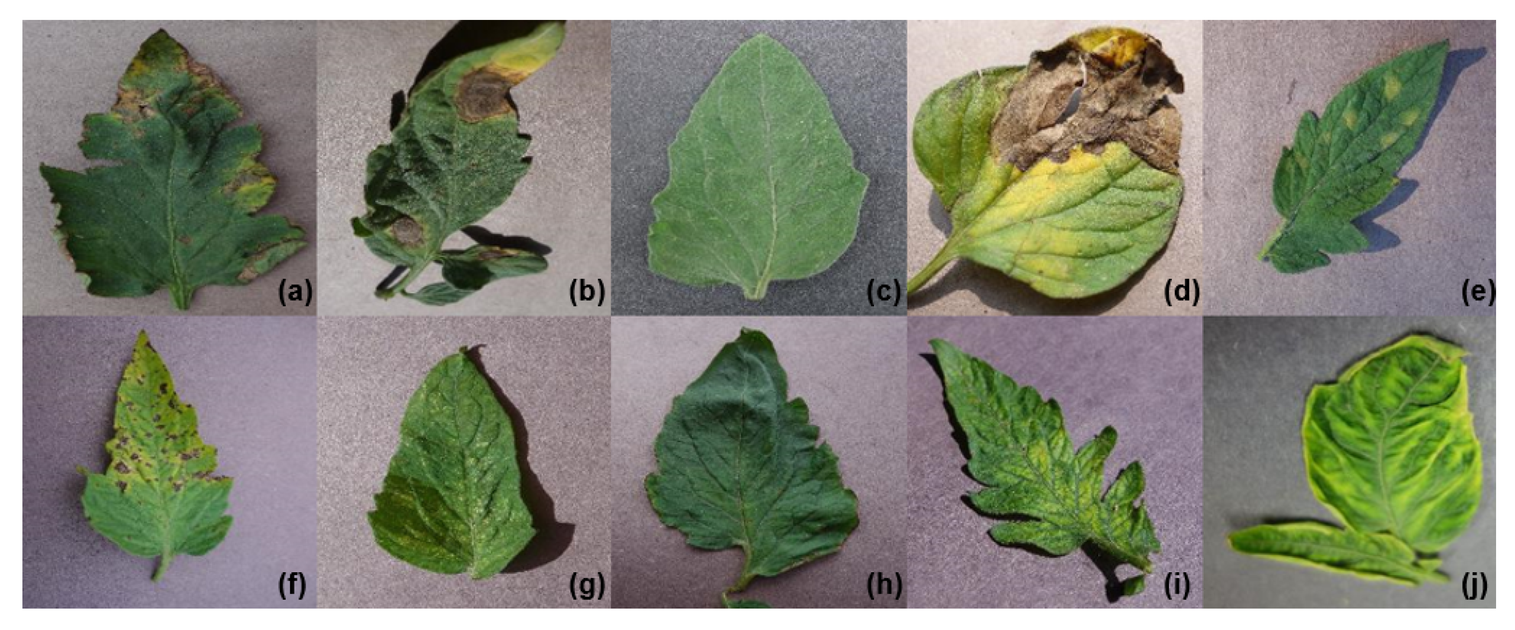
Figure 1 shows one example of each sample class, and
Table 2 gives a summary of our dataset. The total number of images in our dataset is 18,160, divided into nine diseases and a healthy class. All the images used in this work were already cropped to be 224 × 224 or 299 × 299, according to the network input size. Finally, the data was separated into two sets, containing 80% of the data in the training set and the remaining 20% in the testing set. The choice of the split is based on Mohanty et al.’s proposal [
16].
3.2. Data Training
In this phase, the training of the CNNs was carried out through the dataset, ImageNet (contained by 1.2 million images belonging to 1000 categories), with the objective of initializing the weights before the training on this tomato dataset. On the next stage, we took the advantage of Transfer Learning [
28], which aims to transfer knowledge from one or more domains and apply the knowledge to another domain with a different target task. The fine-tuning is a transfer learning concept, which consists on replacing the pre-trained output layer with a layer containing the number of classes of the tomato dataset.
For this work, the last three layers are replaced: a fully-connected layer, a softmax layer, and a classification output layer. The main purpose of using pre-trained CNN models is related to the fast and easy training of a CNN using randomly initialized weights [
29], as well achievement of lower training error than ANNs that are not pre-trained [
30].
The performance of the following CNN architectures have been evaluated for the tomato plant classification problem.
Next, the CNNs assessed will be described.
3.2.1. AlexNet
AlexNet was proposed by Alex Krizhevsky et al. [
8]. In 2012, the CNN model won the most difficult challenge, where ImageNet Large Scale Visual Recognition (ILSVRC) [
31] evaluates algorithms for object detection and image classification at large scale. AlexNet, which has 60 million parameters and 650,000 neurons, consists of five convolutional layers and three fully-connected layers. The first two convolutional layers are followed by normalization and a max-pooling layer, the third and fourth are connected directly, and the fifth convolutional layer is followed by a max-pooling layer. The output goes into a series of two fully-connected layers, in which the second fully-connected layer feed into a softmax classifier. In order to prevent overfitting in the fully-connected layers, the authors employed a regularization method called “dropout” with a ratio of 0.5 [
32]. Another feature of the AlexNet model is the use of Rectified Linear Unit (ReLU), which is applied to each of the first seven layers. The authors mentioned that using ReLU Nonlinearity could train much faster than using the saturating activation functions of Tanh and Sigmoid.
3.2.2. GoogleNet
GoogleNet is presented in the work of Szegedy et al. [
9] and was the winner of ILSVRC in 2014. GoogleNet possesses seven million parameters and contains nine inception modules, four convolutional layers, four max-pooling layers, three average pooling layers, five fully-connected layers, and three softmax layers for the main auxiliary classifiers in the network [
33]. In addition, it uses dropout regularization in the fully-connected layer and applies ReLU activation in all of the convolutional layers. However, this network is much deeper and wider, with 22 total layers, but has a much lower number of network parameters compared to AlexNet. A more detailed explanation of all the relevant parameters of GoogleNet model can be found in the original paper [
9].
3.2.3. Inception V3
Inception V3 [
10] is a deep convolutional architecture widely used for classification tasks. The model concept was introduced by Szegedy in the GoogleNet architecture, where Inception V3 was proposed by updating the inception module [
34]. The Inception V3 network has multiple symmetric and asymmetric building blocks, where each block has several branches of convolutions, average pooling, max-pooling, concatenated, dropouts, and fully-connected layers. This network has 42 total layers and possesses 29.3 million parameters, which means that the computational cost is only about 2.5 higher than GoogleNet. Finally, the authors concluded that the combination of lower parameter count and additional regularization with batch normalized auxiliary classifiers label smoothing allows training of a high quality network on a relatively modest-sized training sets [
10].
3.2.4. Residual Network (ResNet)
The ResNet models, which are based on deep architectures that have shown good convergence behaviors and compelling accuracy, were developed by He et al. [
11]. Based on this, they won first place in the ILSVRC and Common Objects in Context (COCO) classification challenge in 2015. ResNet was built by several stacked residual units and developed with many different numbers of layers: 18, 34, 50, 101, 152, and 1202. However, the number of the operations can be varied depending on the different architectures [
11]. For all of the above, the residual units are composed of convolutional, pooling, and layers. ResNet is similar to VGG net [
23], but ResNet is about eight times deeper than VGG [
34]. The ResNet 18 represents a good compensation between the depth and performance, and this network is composed by five convolutional layers, one average pooling, and a fully-connected layer with a softmax. ResNet 50 contains 49 convolutional layers and a fully-connected layer at the end of the network. Finally, for saving computing resources and training time, ResNet 18 and ResNet 50 were chosen for the development of this work.
3.2.5. CNN Settings
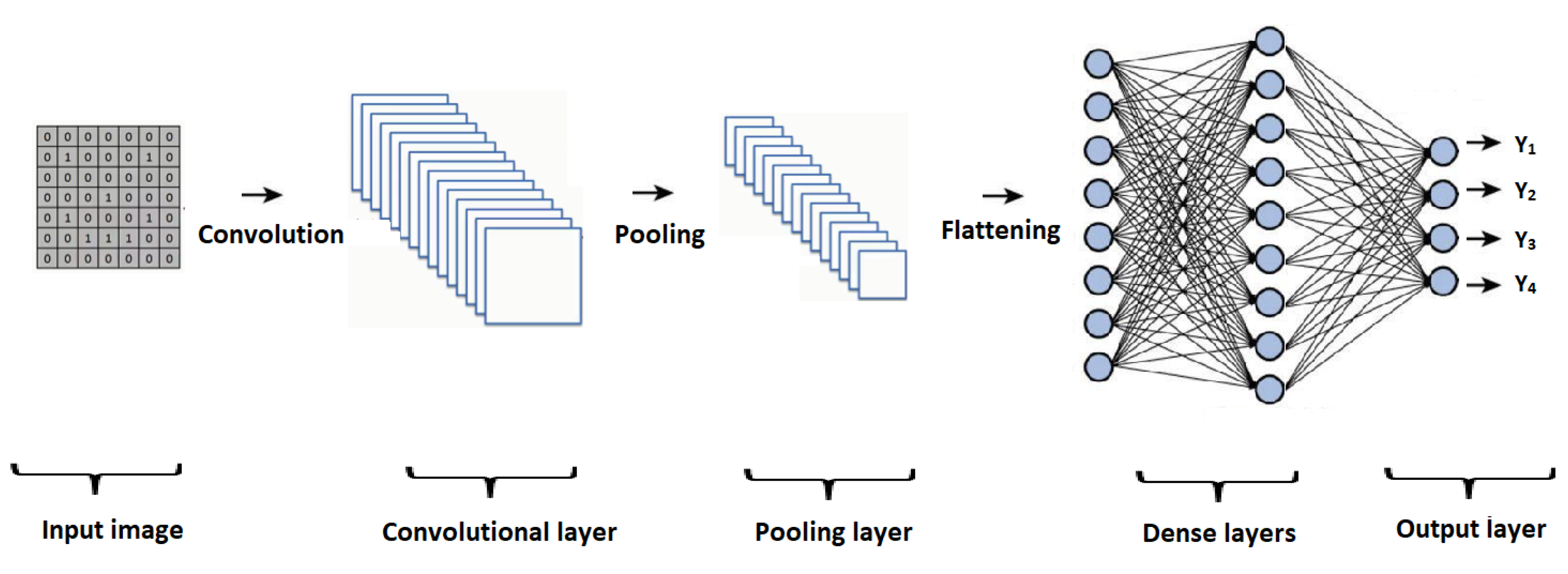
The CNN settings usually consist of a series of specific elements, which are the ones that present the variations in the different architectures.
Figure 2 graphically presents the general architecture of a CNN, with its main elements, such as the input layer, convolutional layer, pooling layer, and a process of flattening, where the information is entered into a set of dense layers, representing the result obtained in the output layer.
Therefore, the characteristics of the architectures used are described in the
Table 3.
To allow a fair comparison between the experiments, an attempt to standardize the hyper-parameters across the experiments was also made, using the following hyper-parameters, which are described in
Table 4.
DL has significantly advanced in many research areas. Stochastic Gradient Descent (SGD) has become the dominant optimization algorithm, proved to be an appropriate trade off between the accuracy and efficiency [
35]. The SGD is simple and effective, and it requires a tuning of the model hyper-parameters, particularly the initial learning rate, which is used in the optimization since it determines how fast the weights are adjusted in order to get a local or global minimum of the loss function. The momentum helps to accelerate SGD in the suitable direction and dampens oscillations [
36]. In addition, the regularization is a very important technique to prevent the overfitting. The most common type of regularization is L2 Regularization, where the combination with SGD results in weight decay, in which each update the weights are scaled by a factor lightly smaller than one [
37]. Each experiment runs a total of 30 epochs, where each epoch is the number of the training iteration. The choice was made due to the results of Mohanty et al.’s proposal [
16] because of its consistently converging after the first step down in the learning rate. Finally, all the CNNs are trained with the batch size of 32.
Training these CNN architectures is extremely computationally intensive. Therefore, all the experiments are carried out on a workstation, presenting the details summarized in
Table 5. The training process was conducted by MATLAB 2018b with Deep Learning (DL) Toolbox, which provides a framework to design and implement CNNs, where applications and graphics help to visualize network activations and monitor the progress of network training. Meanwhile, the statistical analysis of each architecture was carried out with the free software R (version 3.5.2) with its pROC and caret package.
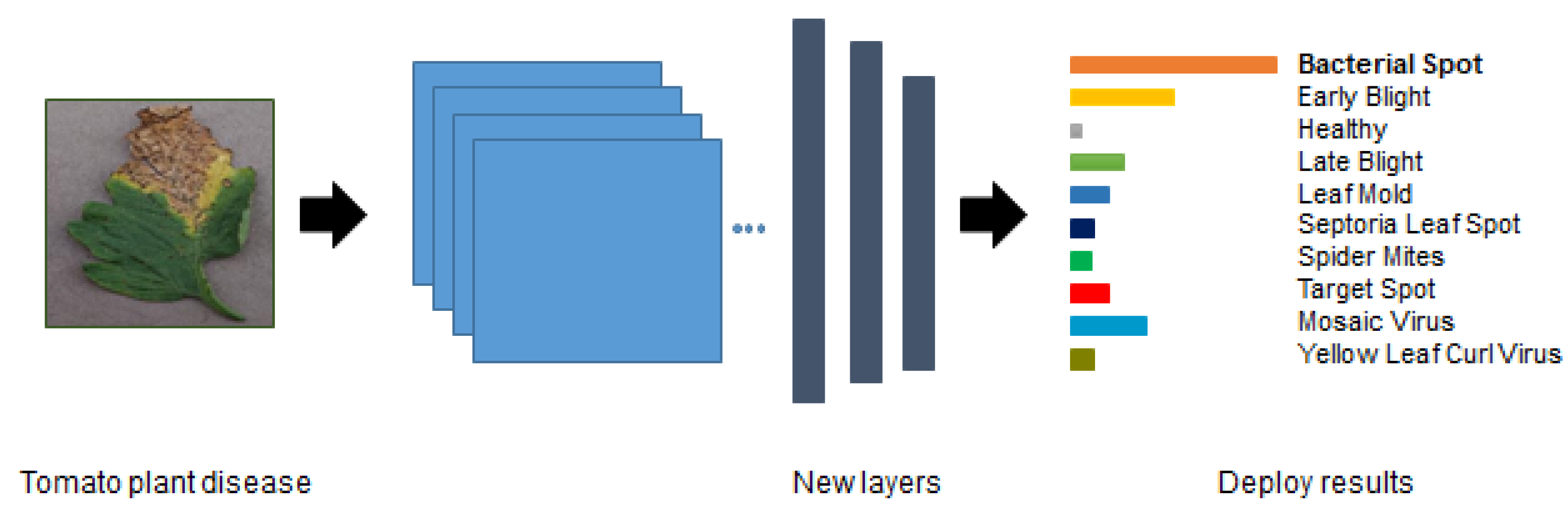
3.3. Data Classification
The number of the classification output layer is equal to the number of the classes. Then, each output has a different probability for the input image because these kind of models have the ability to automatically learn features during the training stage; then, the model picks the highest probability as its prediction of the the class. Finally, this phase determines which disease is present in the leaf using the pre-trained set.
Figure 3 shows an example of the fine-tuning process where the three final layers were replaced by our classification task.
3.4. Evaluation
The performance of the proposed method is evaluated by comparing the pre-trained models with different metrics. The quality of the learning algorithms is generally evaluated by analyzing how well they perform on a test data [
38]. The first one is the Receiver Operating Characteristic Curve (ROC), known as Area Under the Curve (AUC), which is a widely used performance measure in the supervised classification, and it is based on the relation between sensitivity and specificity [
39]. For this work, was used a generalization of the AUC for multiple classes. This function defined by Hand and Till [
40] performs multiclass AUC, and it is composed by the mean of several AUC values. A data frame passes as predictor, and the columns have to be named according to the levels of the response.
The sensitivity or recall corresponds to the accuracy of positive examples, and it refers to how many examples of the positive classes were labeled correctly; this can be calculated with Equation (
1), where
refers to the true positives, which are the number of instances that are positive and are correctly identified, and
represents the false negatives, which are the number of positive cases that are mis-classified as negative.
Specificity corresponds to the conditional probability of true negatives given a secondary class, which means that it approximates the probability of the negative label being true; it is represented by Equation (
2), where
is the number of true negatives or negative cases that are negative and classified as negative, and
is the number of false positives, defined by the negative instances that are incorrectly classified as positive cases.
In general, sensitivity and specificity evaluates the effectiveness of the algorithm on a single class, positive and negative respectively.
Commonly, accuracy is the most used metric to evaluate the classification performance. In the evaluation stage, the accuracy was calculated every 20 iterations. This metric calculates the percentage of samples that are correctly classified, and it is represented in Equation (
3):
Precision, defined as the number of true positives divided by the number of true positives plus the number of false positives, is given by Equation (
4). This measure is about correctness, i.e., it evaluates the predictive power of the algorithm. Precision is how “precise” the model is out of those predicted positive and how many of them are actually positive.
F-score is determined as the harmonic mean precision and recall, as shown in Equation (
5). It focuses on the analysis of positive class. A high value of this metric indicates that the model performs better on the positive class.
4. Results
In this study, an assessment of state-of-the-art pre-trained models for the task of classification of tomato plant diseases using images was done. The objective of this research was to compare the CNN models evaluating the accuracy, precision, sensitivity, specificity, F-Score, and AUC by fine-tuning. The results are shown in
Table 6.
All of the models showed a similar and statistically significant performance. Starting with the AUC, Inception V3 and ResNet 18 had the lower results with 99.2%, followed closely by AlexNet with 99.28%, ResNet 50 with 99.55%, and the best AUC result with GoogleNet, which obtained 99.72%, representing an almost excellent classification. On the other hand, in the accuracy metric, Inception V3 obtained the lower result with 98.65%, followed by AlexNet, ResNet 18, and ResNet 50 with 98.93%, 99.06%, and 99.1 5%, respectively, and the highest result was obtained by GoogleNet with 99.39%. In the same way, the order of the precision results were equal to the previous measure, where the lower percentage was obtained by Inception V3 with 98.28% and the highest by GoogleNet with 99.26%. Finally, in the sensitivity, specificity, and F-score measurements, the new Inception V3 performance was poor with 97.84%, 99.84%, and 98.05%, correspondingly, in opposition to GoogleNet, which got the best percentage in the previous metrics with 99.12%, 99.93%, and 99.20%, respectively. Indeed, as is shown, all of them achieved statistically significant performance in each measure, but the GoogleNet implementation achieved the highest percentage. In addition, based on the processing time it took for each CNN to carry out the classification process, AlexNet showed the best performance by taking the shortest time, which implies a better efficiency compared to the other architectures, remarking that its disadvantage in statistical measures is not significant compared to the results of the other CNNs, so it could be considered to sacrifice a minimum decrease in accuracy in exchange for greater processing efficiency.
Furthermore,
Table 7 presents the confusion matrix of the model with the best outcome based on the performance measures, which is GoogleNet. Depending on the results, it is possible to visually evaluate the performance of the classifier and to determine which classes are highlighted by the neurons of the GoogleNet model. The rows are related with the output class, while the columns are related to the true class. The diagonal cells are associated to the observations that are correctly classified, and the off-diagonal cells correspond to the incorrectly classified observations.
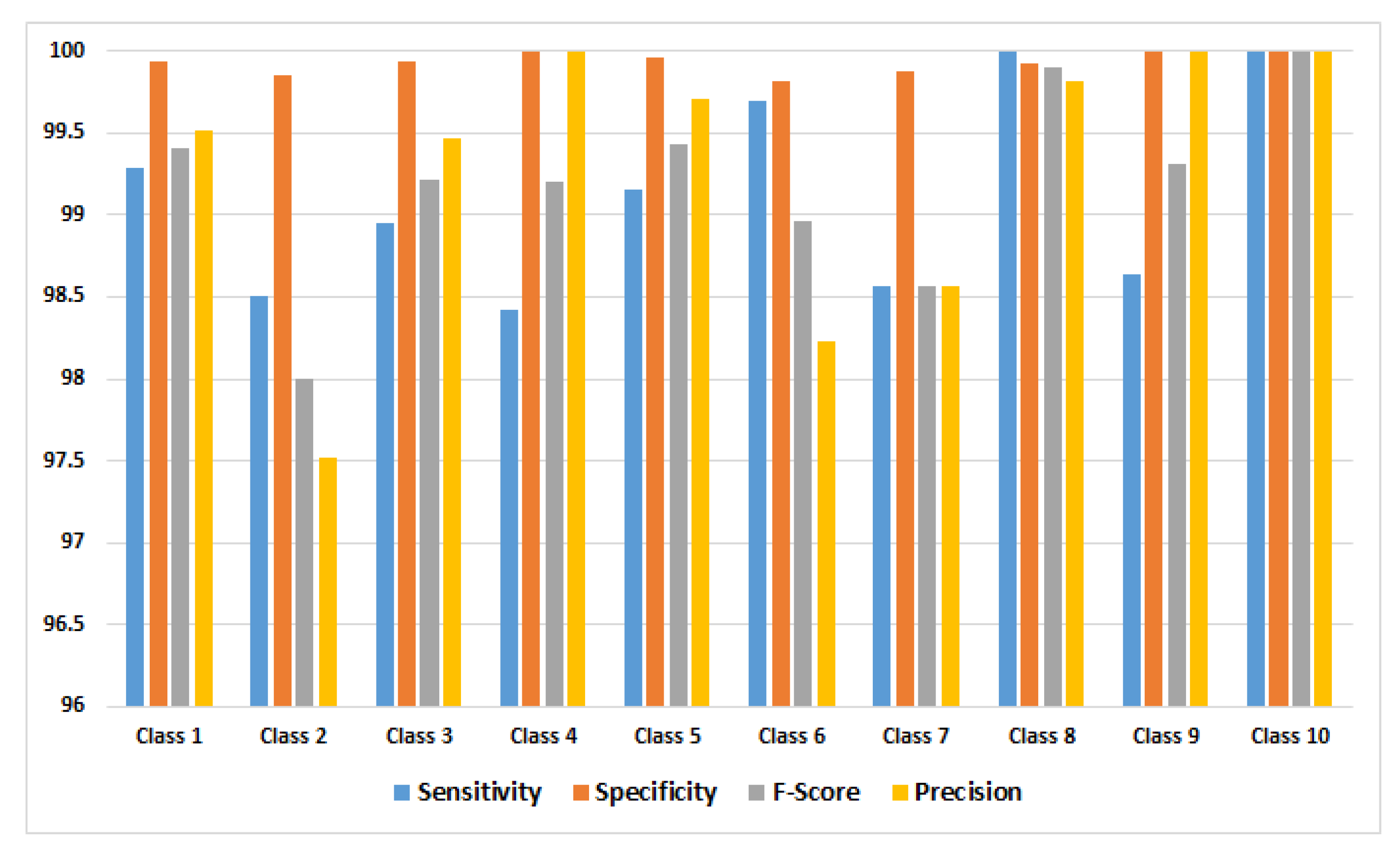
Among the ten classes, two to ten produced 100% correct classification results since those diseases have distinctive appearance and features when compared to the other classes, which are mosaic virus and the healthy class.
Accordingly, the performance measures were calculated for each class, and the obtained results using GoogleNet model are shown in
Figure 4.
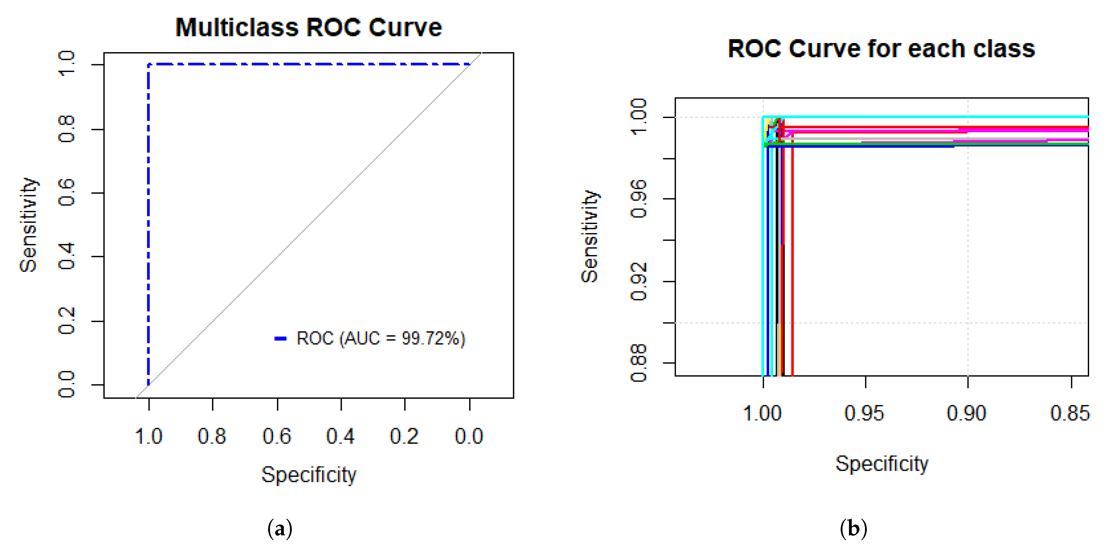
Figure 5a presents the multiclass ROC curve obtained based on the performance of the GoogleNet model with an AUC value of 99.72%. On the other hand,
Figure 5b shows the performance of each class; as shown in the Figure, each class presents a higher fitness.
5. Discussion
DL presents an opportunity to extend research and the application of the basis for classification of plant diseases using digital images. The rapid and accurate models are required to detect the diseases on time. For this work, the dataset used presents nine classes of tomato diseases and a healthy class, which have a total of 18, 160 images. The dataset was divided into 80–20% (training–testing). Therefore, five-state-of-the-art pre-trained models, namely AlexNet, GoogleNet, Inception V3, ResNet 18, and ResNet 50, were trained by the concept of fine-tuning, which consists of replacing the last three layers, where the final output layer has to be compatible with the number of classes.
All of these pre-trained models were evaluated by various metrics: accuracy, precision, sensitivity, specificity, F-Score, and AUC, using the same hyper-parameters. Based on
Table 6, which shows a general result performance, GoogleNet achieved better results than the other architectures. In addition, Inception V3, which is one of the deepest CNN models, shows low performance in
Table 3.
Firstly, a confusion matrix (
Table 7) was achieved, and it shows that two of ten classes produced a 100% rate of correct classifications, representing mosaic virus and the healthy class. Secondly, the performance measures were calculated for each class, in order to know which class obtained lower percentage of the lowest error, based on: sensitivity, specificity, F-Score, and precision, which is because these measurements represent the model performance; it is possible to determine that the classes with the smallest error were: leaf mold, mosaic virus, and the healthy class; the class with greatest error was early blight. All of these were based on the precision metric.
Figure 5 shows that the performance of the GoogleNet model is excellent by the multiclass ROC curve, and it achieves a statistically significant AUC value of 99.72%, which means that the model presented a sensitivity and specificity rate that is able to classify the data with only 0.28% error.
On the other hand, one of the limitations of this work was related to the number of images used. It could be interesting to test the model on a set of images taken under controlled conditions or being able to classify images of diseases as it presents itself on the plant.
In addition, it could be beneficial to create a mobile application that implements the GoogleNet model for an automated diagnosis of tomato plant diseases, so users or farmers with a little or no knowledge can use it to perform their work effectively in the detection of tomato plant diseases.
It is important to mention that training of the models takes a lot of time (around one or two hours on a high performance CPU computer), while the classification is very fast on a Graphics Processing Unit (GPU).
6. Conclusions
This paper proposed a DL method by combining CNN pre-trained models and fine-tuning for the classification of tomato plant diseases. The aim of this work concentrated on comparing the performance of AlexNet, GoogleNet, Inception V3, ResNet 18, and ResNet 50 with different performance metrics. The comparison of these types of models presents the advantages, which are that CNNs do not require any tedious pre-processing, and they have a faster convergence rate and a profitable training performance.
The goal was to find the more suitable model for the task. So, every model used in this work was capable to classify nine diseases in tomato leaves from the healthy class, where the GoogleNet model with 22 layers can reach 99.72% classification of tomato diseases using the training mechanism of transfer learning, which is highly statistically significant and demonstrates the effectiveness of classifying crop diseases with the combination of CNN and fine-tuning adjustment.
On the other hand, Inception V3 obtained the lowest performance compared to the other architectures, presenting a poor architecture despite its large number of layers. It is expected that the proposed method will make an important contribution to the agriculture area.
Author Contributions
Conceptualization, C.E.G.-T. and C.A.O.-O.; Data curation, V.M.-G., C.E.G.-T. and J.M.C.-P.; Formal analysis, V.M.-G., C.E.G.-T. and L.A.Z.-C.; Funding acquisition, C.A.O.-O.; Investigation, C.E.G.-T.; Methodology, V.M.-G., C.E.G.-T. and H.L.-G.; Project administration, C.E.G.-T. and C.A.O.-O.; Resources, J.M.C.-P. and H.G.-R.; Software, V.M.-G., H.G.-R., H.L.-G., R.M.-Q. and C.A.G.M.; Supervision, J.I.G.-T. and C.A.G.M.; Validation, V.M.-G., C.E.G.-T., L.A.Z.-C. and J.I.G.-T.; Visualization, C.E.G.-T. and H.L.-G.; Writing—original draft, V.M.-G., C.E.G.-T., L.A.Z.-C., J.M.C.-P., J.I.G.-T., H.G.-R. and R.M.-Q.; Writing—review & editing, C.E.G.-T., L.A.Z.-C., J.M.C.-P., J.I.G.-T. and H.G.-R. All authors have read and agreed to the published version of the manuscript.
Funding
This research received no external funding.
Conflicts of Interest
The authors declare no conflict of interest.
References
- SAGARPA. Planeación Agrícola Nacional 2017–2030. Available online: https://www.gob.mx/sagarpa/documentos/planeacion-agricola-nacional-2017-2030 (accessed on 15 December 2018).
- Hanssen, I.M.; Lapidot, M. Major tomato viruses in the Mediterranean basin. In Advances in Virus Research; Academic Press: Oxford, UK, 2012; Volume 84, pp. 31–66. [Google Scholar]
- Brahimi, M.; Boukhalfa, K.; Moussaoui, A. Deep learning for tomato diseases: classification and symptoms visualization. Appl. Artif. Intell. 2017, 31, 299–315. [Google Scholar] [CrossRef]
- Barbedo, J.G. Factors influencing the use of deep learning for plant disease recognition. Biosyst. Eng. 2018, 172, 84–91. [Google Scholar] [CrossRef]
- Al-Hiary, H.; Bani-Ahmad, S.; Reyalat, M.; Braik, M.; ALRahamneh, Z. Fast and accurate detection and classification of plant diseases. Int. J. Comput. Appl. 2011, 17, 31–38. [Google Scholar] [CrossRef]
- Brahimi, M.; Arsenovic, M.; Laraba, S.; Sladojevic, S.; Boukhalfa, K.; Moussaoui, A. Deep Learning for Plant Diseases: Detection and Saliency Map Visualisation. In Human and Machine Learning; Springer International Publishing: Cham, Switzerland, 2018; pp. 93–117. [Google Scholar]
- Ferentinos, K.P. Deep learning models for plant disease detection and diagnosis. Comput. Electron. Agric. 2018, 145, 311–318. [Google Scholar] [CrossRef]
- Krizhevsky, A.; Sutskever, I.; Hinton, G.E. Imagenet classification with deep convolutional neural networks. In Advances in Neural Information Processing Systems; Curran Associates, Inc.: New York, NY, USA, 2012; pp. 1097–1105. [Google Scholar]
- Szegedy, C.; Liu, W.; Jia, Y.; Sermanet, P.; Reed, S.; Anguelov, D.; Erhan, D.; Vanhoucke, V.; Rabinovich, A. Going deeper with convolutions. In Proceedings of the IEEE Conference on Computer Vision and Pattern Recognition, Boston, MA, USA, 7–12 June 2015; pp. 1–9. [Google Scholar]
- Szegedy, C.; Vanhoucke, V.; Ioffe, S.; Shlens, J.; Wojna, Z. Rethinking the inception architecture for computer vision. In Proceedings of the IEEE Conference on Computer Vision and Pattern Recognition, Las Vegas, NV, USA, 26 June–1 July 2016; pp. 2818–2826. [Google Scholar]
- He, K.; Zhang, X.; Ren, S.; Sun, J. Deep residual learning for image recognition. In Proceedings of the IEEE Conference on Computer Vision and Pattern Recognition, Las Vegas, NV, USA, 26 June–1 July 2016; pp. 770–778. [Google Scholar]
- Kawasaki, Y.; Uga, H.; Kagiwada, S.; Iyatomi, H. Basic study of automated diagnosis of viral plant diseases using convolutional neural networks. In International Symposium on Visual Computing; Springer: Cham, Switzerland, 2015; pp. 638–645. [Google Scholar]
- Jia, Y.; Shelhamer, E.; Donahue, J.; Karayev, S.; Long, J.; Girshick, R.; Guadarrama, S.; Darrell, T. Caffe: Convolutional architecture for fast feature embedding. In Proceedings of the 22nd ACM international conference on Multimedia, Orlando, FL, USA, 3–7 November 2014; pp. 675–678. [Google Scholar]
- Fujita, E.; Kawasaki, Y.; Uga, H.; Kagiwada, S.; Iyatomi, H. Basic investigation on a robust and practical plant diagnostic system. In Proceedings of the 2016 15th IEEE International Conference on Machine Learning and Applications (ICMLA), Anaheim, CA, USA, 18–20 December 2016; pp. 989–992. [Google Scholar]
- Sladojevic, S.; Arsenovic, M.; Anderla, A.; Culibrk, D.; Stefanovic, D. Deep neural networks based recognition of plant diseases by leaf image classification. Comput. Intell. Neurosci. 2016, 2016, 3289801. [Google Scholar] [CrossRef] [Green Version]
- Mohanty, S.P.; Hughes, D.P.; Salathé, M. Using deep learning for image-based plant disease detection. Front. Plant Sci. 2016, 7, 1419. [Google Scholar] [CrossRef] [Green Version]
- Hughes, D.; Salathé, M. An open access repository of images on plant health to enable the development of mobile disease diagnostics. arXiv 2015, arXiv:1511.08060. [Google Scholar]
- Nachtigall, L.G.; Araujo, R.M.; Nachtigall, G.R. Classification of apple tree disorders using convolutional neural networks. In Proceedings of the 2016 IEEE 28th International Conference on Tools with Artificial Intelligence (ICTAI), San Jose, CA, USA, 6–8 November 2016; pp. 472–476. [Google Scholar]
- DeChant, C.; Wiesner-Hanks, T.; Chen, S.; Stewart, E.L.; Yosinski, J.; Gore, M.A.; Nelson, R.J.; Lipson, H. Automated identification of northern leaf blight-infected maize plants from field imagery using deep learning. Phytopathology 2017, 107, 1426–1432. [Google Scholar] [CrossRef] [Green Version]
- Lu, Y.; Yi, S.; Zeng, N.; Liu, Y.; Zhang, Y. Identification of rice diseases using deep convolutional neural networks. Neurocomputing 2017, 267, 378–384. [Google Scholar] [CrossRef]
- Huang, G.; Liu, Z.; Van Der Maaten, L.; Weinberger, K.Q. Densely connected convolutional networks. In Proceedings of the IEEE Conference on Computer Vision and Pattern Recognition, Honolulu, HI, USA, 21–26 July 2017; pp. 4700–4708. [Google Scholar]
- Iandola, F.N.; Han, S.; Moskewicz, M.W.; Ashraf, K.; Dally, W.J.; Keutzer, K. Squeezenet: Alexnet-level accuracy with 50x fewer parameters and <0.5 mb model size. arXiv 2016, arXiv:1602.07360. [Google Scholar]
- Simonyan, K.; Zisserman, A. Very deep convolutional networks for large-scale image recognition. arXiv 2014, arXiv:1409.1556. [Google Scholar]
- Wang, G.; Sun, Y.; Wang, J. Automatic image-based plant disease severity estimation using deep learning. Comput. Intell. Neurosci. 2017, 2017, 2917536. [Google Scholar] [CrossRef] [PubMed] [Green Version]
- Wang, J.; Chen, L.; Zhang, J.; Yuan, Y.; Li, M.; Zeng, W. CNN Transfer Learning for Automatic Image-Based Classification of Crop Disease. In Chinese Conference on Image and Graphics Technologies; Springer: Singapore, 2018; pp. 319–329. [Google Scholar]
- Rangarajan, A.K.; Purushothaman, R.; Ramesh, A. Tomato crop disease classification using pre-trained deep learning algorithm. Procedia Comput. Sci. 2018, 133, 1040–1047. [Google Scholar] [CrossRef]
- Khandelwal, I.; Raman, S. Analysis of Transfer and Residual Learning for Detecting Plant Diseases Using Images of Leaves. In Computational Intelligence: Theories, Applications and Future Directions-Volume II; Springer: Singapore, 2019; pp. 295–306. [Google Scholar]
- Pan, S.J.; Yang, Q. A survey on transfer learning. IEEE Trans. Knowl. Data Eng. 2010, 22, 1345–1359. [Google Scholar] [CrossRef]
- Deniz, E.; Şengür, A.; Kadiroğlu, Z.; Guo, Y.; Bajaj, V.; Budak, Ü. Transfer learning based histopathologic image classification for breast cancer detection. Health Inf. Sci. Syst. 2018, 6, 18. [Google Scholar] [CrossRef] [PubMed]
- Dahl, G.E.; Yu, D.; Deng, L.; Acero, A. Context-dependent pre-trained deep neural networks for large-vocabulary speech recognition. IEEE Trans. Audio Speech Lang. Process. 2012, 20, 30–42. [Google Scholar] [CrossRef] [Green Version]
- Russakovsky, O.; Deng, J.; Su, H.; Krause, J.; Satheesh, S.; Ma, S.; Huang, Z.; Karpathy, A.; Khosla, A.; Bernstein, M.; et al. ImageNet Large Scale Visual Recognition Challenge. Int. J. Comput. Vis. (IJCV) 2015, 115, 211–252. [Google Scholar] [CrossRef] [Green Version]
- Zhang, K.; Wu, Q.; Liu, A.; Meng, X. Can Deep Learning Identify Tomato Leaf Disease? Adv. Multimed. 2018, 2018, 6710865. [Google Scholar] [CrossRef] [Green Version]
- Ghazi, M.M.; Yanikoglu, B.; Aptoula, E. Plant identification using deep neural networks via optimization of transfer learning parameters. Neurocomputing 2017, 235, 228–235. [Google Scholar] [CrossRef]
- Too, E.C.; Yujian, L.; Njuki, S.; Yingchun, L. A comparative study of fine-tuning deep learning models for plant disease identification. Comput. Electron. Agric. 2018, 161, 272–279. [Google Scholar] [CrossRef]
- Kleinberg, R.; Li, Y.; Yuan, Y. An Alternative View: When Does SGD Escape Local Minima? arXiv 2018, arXiv:1802.06175. [Google Scholar]
- Ruder, S. An overview of gradient descent optimization algorithms. arXiv 2016, arXiv:1609.04747. [Google Scholar]
- van Laarhoven, T. L2 regularization versus batch and weight normalization. arXiv 2017, arXiv:1706.05350. [Google Scholar]
- Japkowicz, N.; Shah, M. Evaluating Learning Algorithms: A Classification Perspective; Cambridge University Press: Cambridge, UK, 2011. [Google Scholar]
- Hanley, J.A.; McNeil, B.J. The meaning and use of the area under a receiver operating characteristic (ROC) curve. Radiology 1982, 143, 29–36. [Google Scholar] [CrossRef] [PubMed] [Green Version]
- Hand, D.J.; Till, R.J. A simple generalisation of the area under the ROC curve for multiple class classification problems. Mach. Learn. 2001, 45, 171–186. [Google Scholar] [CrossRef]
© 2020 by the authors. Licensee MDPI, Basel, Switzerland. This article is an open access article distributed under the terms and conditions of the Creative Commons Attribution (CC BY) license (http://creativecommons.org/licenses/by/4.0/).


 ,
, 


