Research on Short-Term Wind Power Forecasting by Data Mining on Historical Wind Resource

1
Key Laboratory of Intelligent Manufacturing Technology, Ministry of Education, Shantou University, Shantou 515063, China
2
Institute of Energy Science, Shantou University, Shantou 515063, China
*
Author to whom correspondence should be addressed.
Appl. Sci. 2020, 10(4), 1295; https://0-doi-org.brum.beds.ac.uk/10.3390/app10041295
Submission received: 11 January 2020
/
Revised: 11 February 2020
/
Accepted: 11 February 2020
/
Published: 14 February 2020
(This article belongs to the Special Issue Machine Learning for Energy Forecasting)
Abstract
:In order to enhance the accuracy of short-term wind power forecasting (WPF), a short-term wind power forecasting method based on historical wind resources by data mining has been designed. Firstly, the spoiled data resulting from wind turbine and meteorological monitoring equipment is eliminated, and the missing data is added by the Lomnaofski optimization model, which is based on the temporal-spatial correlation of meteorological data. Secondly, the wind characteristics are analyzed by the continuous time similarity clustering (CTSC) method, which is used to select similar samples. To improve the accuracy of deterministic prediction and prediction error, the radial basis function neural network (RBF) deterministic forecasting model was built, which can approximate nonlinear solutions. In addition, the wind power interval prediction method, combining fuzzy information granulation and an Elman neural network (FIG-Elman), is proposed to acquire forecasting intervals. The deterministic prediction of the RBF-CTSC model has high accuracy, which can accurately describe the randomness, fluctuation and nonlinear characteristics of wind speed. Additionally, the mean absolute error (MAE) and root mean square error (RMSE) are reduced by the new model. The interval prediction of FIG-Elman results show that the interval width decreased by 18.85%, and the coverage probability of interval increased by 10.94%.
1. Introduction
With the rapid development and large-scale integration of wind power, accurate and reliable wind power forecasting (WPF) plays a key role in helping power system operators and market operators to schedule and trade wind generation at various spatial and temporal scales. Highly penetrated and correlated wind power integrated into the power system implies great uncertainties and technical challenges for system operators. Therefore, short-term WPF is one of the most important solutions to promote the development of wind energy, with the advantages of helping electric dispatching and restraining the impact of fluctuations of wind power effectively.
Most of the existing WPF methods have been optimized by hybrid different algorithms in recent years. Reference [1] evaluated the effectiveness of autoregressive moving average–generalized autoregressive conditional heteroscedasticity (ARMA–GARCH) approaches for modeling the mean and volatility of wind speed. Reference [2] analyzed the Kalman filter to the configuration for wind speed and wind power forecast, while reference [3] proposed a real-time forecasting method of wind speed based on spatio-temporal correlation and the BP neural network, which improved the prediction accuracy. Besides, in the literature [4,5,6,7], the optimization and combination of the neural network algorithm, empirical mode decomposition and regression vector machine were used to predict wind power. Even though the combination forecasting model improved forecasting accuracy to some extent, the results were still unsatisfactory. After in-depth research, we find scholars have been paying attention to researching WPF while screening the similar set as prediction samples referring to the data mining and fine-analysis of samples. According to the analysis principles, the existing analysis methods based on data mining and identifying similar samples are divided into three:
- Predicting periodicity based on monthly or quarterly historical meteorological conditions [8];
- Classification of meteorological data by clustering algorithms according to similar wind conditions, weather patterns and output patterns [9]; and
- Application of distance function and entropy correlation based on the characteristics of wind speed to obtain similar samples [10].
While most works have looked at how to predict wind power generation at a given site or for a given portfolio, only few have considered the spatio-temporal correlation in their power generation. Research on the methods above indicate that the training samples are mostly selected from historical data, with a definite aim and limited number to study a similar set. However, there are lots of redundant data in samples, on account of ignoring the diversity of meteorological data changes and the continuity of wind speed in a short time. The problem we have outlined deals largely with the study of data pre-processing. It is necessary to combine the variability of actual weather conditions and the continuity of short times to obtain the accurate sample data, so as to improve the accuracy of forecasting through the intentionally screened and fine-analysis of historical data.
In this paper, we focus on original data preprocessing, which includes removing redundant data and supplementing missing data. This is not because redundant data will lead to much more calculational burden and slow down the calculation speed, but because missing data may cause the loss of effective information and reduce the prediction accuracy. To improve the accuracy of WPF, it is important to consider the spatio-temporal correlation between the meteorological data in the same time series when supplementing the missing data.
To solve these problems, we present a short-term WPF approach based on the data mining of historical wind sources. The paper is organized as follows. Section 2 describes the structure of the Lomnaofski optimization model, which is used to pre-process the data. The continuous time similarity clustering method (CTSC) is introduced in Section 3. The numeral case of single point prediction solved by the RBF network and interval prediction solved by the FIG-Elman model are presented and discussed in Section 4 and Section 5, respectively, followed by the conclusion. The results show that the short-term prediction accuracy of wind power has improved.
2. Lomnaofski Optimization Model
In this section, we describe the improved Lomnaofski model for data pre-processing. The power output of wind turbines is stochastic, which is determined by wind and wind turbine generators. At the same time, the bad points and missing values of historical wind sources will be produced by wind turbines and meteorological monitoring equipment. It is necessary to effectively eliminate the spoiled data and supplement missing data in order to fully study the correlation between meteorological data and power data.
The Lomnaofski norm is a criterion to distinguish the singular point of measured data, which can establish basic composite numerical statistical analysis theory and eliminate abnormal data. Considering the characteristics of wind speed and correlation of time series, the Lomnaofski norm is selected to preprocess meteorological data such as wind speed.
The Lomnaofski norm is based on the measurements conformed to the t-distribution. In a certain number of measurements, n, the equal-precision measurement obtains a group of data, . If there is spoiled data, , which needs to be supplemented after eliminating, then delete it. The optimization model is discriminated and processed as follows:
- Remove the spoiled data, , then calculate the arithmetic average in the measurements without . is written as:
- Calculate the standard deviation , except the residuals of , which is expressed as:
- The coefficient value, , is obtained from the t distribution table according to the selected significant level A and the number of measurements n, .
- If , then is determined to be an abnormal point and should be eliminated; if , it means that is normal data and should be retained.
- The data which is eliminated or missed is supplemented by using the value before and after the spoiled data in the same sequence, which is expressed as . If the value before and after the spoiled data is also missed, then it is supplemented according to the spatial correlation sequence obtained by the synchronization monitoring, which is expressed as , where is the correlation coefficient of two spatial sequences, and is the corresponding point of the spatial correlation sequence.
Wind speed and wind direction data sequences are mainly preprocessed in this paper. The preprocessed data obtained by the optimized model is shown in Figure 1. As can be seen in Figure 1, the wind farm has obvious characteristics of randomness, fluctuation and nonlinearity. The samples can be preprocessed effectively by the Lomnaofski optimization model.
3. Similar clustering Analysis Method Based on Continuous Periods
Most of existing articles which have considered the diurnal similarity of wind speed changes are shown below. Reference [11] used the extreme difference method to analyze the similarity of the main parameters affecting wind power, and established a Chebyshev neural network model for power prediction whose accuracy was higher than that of only using a neural network. In reference [12], a neural network model was constructed based on principal component analysis, which had the advantage of eliminating the relationship among the factors affecting the original wind power. The results showed that the prediction accuracy had been improved. Reference [13] established a variety of prediction models according to the meteorological conditions, and the prediction effect was better when the meteorological conditions were stable. In reference [14], the meteorological data of predicted time points were used as the core of the gray correlation method to cluster similar days, and meteorological parameters were analyzed to reduce dimension, obtain independent factors and establish a prediction model. Reference [15] established the Elman prediction model based on determining the optimal length of similar time intervals after analyzing historical data and combining the K-means clustering method for power clustering.
The foregoing methods just cluster historical data on similar days monthly or quarterly, so the timescale is long when using historical data for short-term power prediction, which does not consider the continuity of meteorological data in short-time scales such as wind speed, as well as the fluctuation of wind speed, or the mutation and trend of wind speed series. A continuous-time similarity clustering analysis method (CTSC) is proposed in this paper, which uses the similar wind speed series in the same period of N-day as the clustering set, and then selects the time series with high similarity as training samples. The prediction accuracy has been significantly improved due to the high similarity between data samples and prediction sets such as wind speed and wind direction.
There are two points that need to be taken into consideration when selecting continuous periods. The first is the similarity analysis of daily characteristics, which mainly rely on similarities between the parameters of the training set and historical data. The output of wind turbines is affected by wind direction, wind speed, air temperature and air pressure, etc. The relationship of the influence factors can be expressed as follows
where , , , , , are the time of minimum and maximum speed, the time of lowest and highest temperature, and the lowest and highest temperature, respectively. is the average pressure. and are cosine and sinusoidal values of wind direction.
The gray correlation method is used to identify similar days. Let the eigenvectors of the prediction day be . The wind speed association on the j-th day can thus be expressed as
where represents the resolution coefficient, which is generally 0.5.
The eigenvectors of the predicted day and the correlation coefficients of wind direction, , air pressure, , and temperature, , on the j-th day are obtained, and so on. The weight ratio is used to weigh the eigenvector components of similar days. The weight ratio is expressed as follows
where represents the similarity coefficient.
The similar samples are selected from the data samples of the approaching half-month to be predicted during the forecasting.
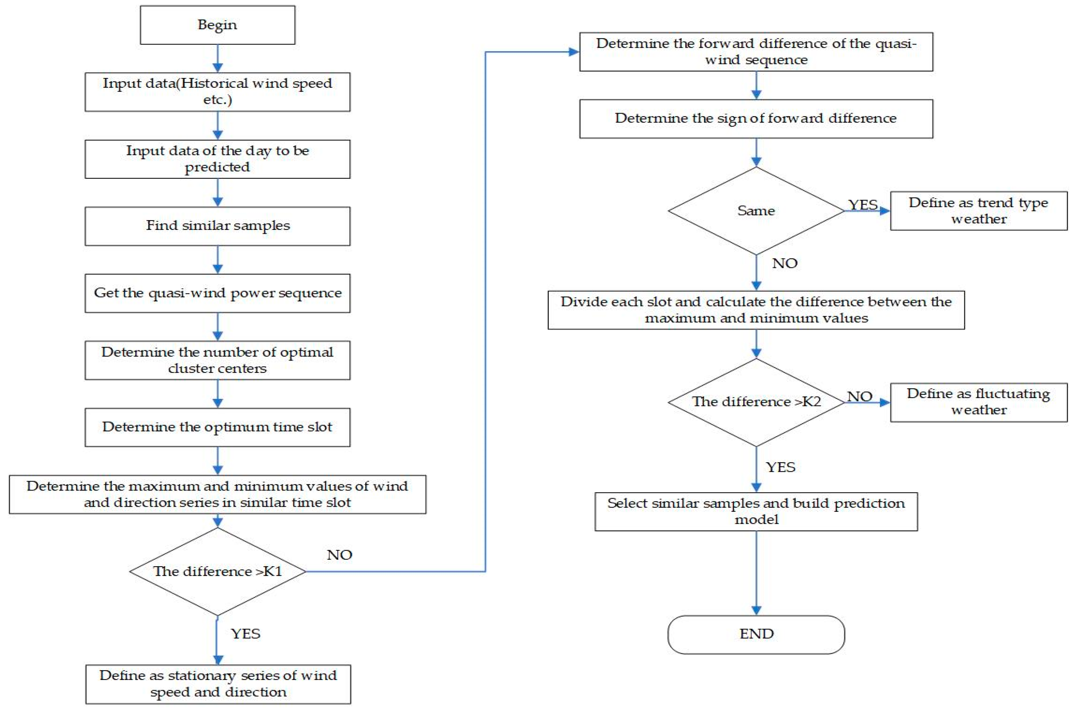
Then, the similar samples obtained after preliminary screening should be finely analyzed according to the shape and similarity of development trends, combined with the number of samples. The days to be predicted are divided into time periods, and the final period length is determined on the premise of meeting the training sample number. The specific methods are as follows:
- Determine the number of the best clustering centers so that they can cover all the samples.
- Determine the length of period, preliminarily by the similarity of shape and development trend of similar days.
- Optimal period length is obtained, and the samples with the above similar characteristics are selected from the similar days, according to the number of clustering centers, and the development trends of the wind speed and wind direction.
- On the premise of meeting the number of training samples, the final length of period is determined.
Different shapes and development trends can be classified into the following categories, considering different states of meteorological changes.
If the input eigenvectors, such as wind speed and wind direction, have few changes in the continuous period, we define it as a stationary stage. The expression is as follows:
If the input eigenvectors, such as wind speed and wind direction, have obvious trend changes in the continuous period, it can be regarded as a trend change. The expression is as follows:
If the input eigenvectors, such as wind speed and wind direction, have continued volatility in the continuous period, it can be regarded as a continuous fluctuation. The expression is as follows
where is the quasi-wind power sequence by cubic operation of the wind speed, , are the maximum and minimum in and is the difference between the maximum and minimum values in the slot. , are the respective set thresholds.
The expressions of and are as follows
where , and are the beginning and the end of , is the maximum point of , is the number of and are the threshold coefficient, which are determined according the specific wind conditions of the wind form. Additionally, is set to 0.5, and is set to 1.
The procedure of partitioning continuous periods based on wind characteristics is shown in Figure 2.
4. Numeral Case of Deterministic Prediction
The establishment of the wind speed prediction model is mainly divided into four parts: data processing; establishing a hybrid model; establishing a comparison model; and verifying the effectiveness of the hybrid model. In this section, we introduce a numeral case of deterministic prediction using the RBF network, considering the characteristics of randomness, fluctuation and nonlinearity of wind speed, and because the RBF network can approximate arbitrary nonlinear functions and has good generalization ability. The RBF neural network has strong nonlinear fitting ability and can map any complex nonlinear relationship. RBF has a three-layer structure, including the input layer, hidden layer and output layer. This paper will not go into detail due to limited space. In this section, we will compare the prediction results of the RBF network and BP neural network.
In order to verify the applicability of the model, the sampling time interval is 10 minutes and the monitoring period is 2018.01.01–2018.08.30. The sampling variables include wind speed, as well as six factors: sinusoidal wind direction (); cosine wind direction (); temperature (T); air pressure (P); humidity (H); and motor speed (M). The data of the first three quarters of the month will be used as a training set, and the remaining data as a testing set after preprocessing. Here, the statistical analysis of data samples excludes extreme weather such as typhoons during the monitoring period. One day is divided into four continuous periods, with each period containing 400 minutes, and one day having 144 measured values of [0–40], [41–80], [80–120] and [120–144], with the corresponding times being [0:00–6:40], [6:40–13:20], [13:20–20:00] and [20:00–24:00]. The forecasting day is 7 February 2019. Firstly, according to the above continuous time similarity clustering method (CTSC), the simultaneous data similar to the test samples are selected and used as the training samples to conduct the training network. The prediction results are shown in Figure 3.
In this section, an RBF network model based on continuous time similarity clustering (CTSC) is proposed, and the results of RBF are better than that of the BP neural network, as shown in Figure 3. In Figure 3a,c, compared with primitive model and the RBF-CTSC model, all have strong fluctuation. The predicted results of the primitive model are far from the measured values. In Figure 3b, the prediction results of the RBF-CTSC model are significantly closer to the measured wind power values than the primitive model. In Figure 3d, compared with the measured values, the prediction results of the primitive model without CTSC lack fluctuation characteristics, and do not reflect the trend of the original series. As we can see from Figure 3, the RBF model is mainly applied to reflect the nonlinear characteristic of wind speed, while the time series model is used to reflect the linear characteristic of wind speed. As can be seen in Figure 3, both models can reflect the fluctuation trends of some actual values, but the prediction results of the RBF network are more approximate to actual values, and the validity of the model is proven. Table 1 is the accuracy analysis of the prediction model, in which MAE and RMSE are the error indexes. The less MAE or RMSE there are, the greater the prediction accuracy is. Comparing the average absolute error (MAE) and root mean square error (RMSE) of these two models, these error indexes of the BP model and RBF-CTSC model show a decreasing trend in order. We also find that even though the wind speed and direction present a randomness and volatility fluctuation range in the training data, the results of the new method still have a good performance. Based on the deterministic WPF, the randomness, fluctuation and nonlinear characteristics of wind power can be described accurately, which can help to optimize the grid scheduling plan and improve the reliability of the wind power grid.
5. Numeral Case of Interval Prediction
At present, we learn that most of WPF methods focus on deterministic prediction. There is a drawback of deterministic prediction, in which the error between the predicted and the measured still exists, so that it is important to study the interval prediction of wind power by which the instability of wind power caused by wind uncertainty can be better described.
In the study of the interval prediction method, reference [16] explored a forecasting method combined empirical mode decomposition and extreme machine learning. Additionally, the forecasting results show that the interval prediction effect is good. Reference [17] proposed an interval prediction model based on the wavelet neural network, optimized by a multi-objective intelligent algorithm. Compared with traditional multi-objective methods, this method has better performance. However, most of the existing forecasting models only output point or interval forecasting separately; it does not provide more detailed information for related staff, which is helpless to the development demand of the energy, Internet and power market [18]. Researchers begin to apply fuzzy information granulation to power prediction, as the maximum and minimum values of the interval prediction can be obtained by such methods. The deterministic and interval prediction results of complex nonlinear time series can be obtained at the same time, which provides a technical support for dispatching [19].
Major existing wind power interval prediction methods have disadvantages such as complex calculation, slow convergence speed and low efficiency. For example, the choice of the Hessian matrix and derivative operations will increase the computational complexity of the model. The Elman neural network belongs to the feedforward neural network, which can approximate any nonlinear function under the given kernel function condition. The estimation of the upper and lower limits of the neural network interval is based on the parameters of the optimized neural network, and does not need prior knowledge and hypothesis estimation, i.e., the lower-upper bound estimation method (LUBE). This paper establishes the Elman neural network wind power interval prediction model based on continuous time similarity clustering.
5.1. LUBE-Elman Interval Prediction
The network structure of the Elman neural network (ENN) is divided into four parts—an input layer, a hidden layer, an undertaking layer and an output layer—as illustrated in Figure 4. The input layer can be used to transmit the raw data; the imported weighted data are mapped linearly or nonlinearly through the transfer function of the hidden layer; and finally, the processed data are performed by the linear weighted method in the output layer. The framework of the LUBE-Elman interval prediction is shown in Figure 4. For the multi-input and dual-output Elman model, the weights and thresholds in the model can be given arbitrarily and selected optimally.
According to the previous method, we obtained similar continuous time intervals from the training samples. The training set is expressed as , where represents the input parameters of the model, including the historical wind speed, wind direction, temperature and pressure, and is the historical wind power. The testing set is expressed as , and then determined given the confidence interval and confidence probability of , where represents confidence, and it is 0.9 in this paper. The prediction interval is .
where means the lower limit of the prediction interval, and means the upper limit of the prediction interval.
The training set and testing set are normalized, and the normalized interval is (0, 1). The normalized expression is as follows:
There are four input eigenvectors and one output vector in the model. Where , and are the weight of the first stage, the weight of the second stage and the weight from the hidden layer to the output layer, respectively. , i = 1,2,3,4, represents the input eigenvector, including wind speed, direction, pressure and temperature. is the K-th value of the eigenvector. is the transfer function of the middle layer neural network. The expression is as follows:
The final output value is the weighted summation of each eigenvector, as follows:
In the training process, the weights and thresholds of the given hidden layer will not be changed, but the parameters of the output layer will be changed. The prediction interval will be obtained from optimal weights based on the calculation by the least square method.
5.2. Interval Prediction Model Based on FIG-Elman
This paper innovatively combines the advantages of the FIG and Elman neural network, including short-term memory function, high sensitivity and dynamic modeling ability. Compared with other WPF methods, the main outstanding points are the point forecasting results, and the interval forecasting results can be obtained simultaneously with quick calculating speed and high working efficiency. Figure 5 is the flow chart of the WPF model, based on FIG-Elman.
The triangular granulation function is used to calculate the content in this paper, with the expression as follows:
5.3. Prediction Interval Evaluation Indicators
The prediction interval indicators include mean absolute percentage error, forecasting interval coverage percentage, forecasting interval width.
- Indicator 1: Mean absolute percentage error (MAPE) is used to evaluate the error between measured and predicted value [20]. The smaller the value, the higher the prediction accuracy. Its expression is as followswhere n represents the number of test samples, represents the measured power value and represents the predicted value.
- Indicator 2: Forecasting interval coverage percentage (FICP) is used to express the probability of the measured value in the prediction interval. A more measured value falls into the interval when the value of is larger, and the reliability of the interval prediction is higher. Its expression is as followswhere , , or .
- Indicator 3: Forecasting interval average width (FIAW) is used to test the appropriateness of the predictive interval width, which used to prevent excessive interval width. The smaller the value is, the narrower the interval is, as followswhere represents the upper limit of the prediction interval of the first prediction sample. denotes the lower limit of the prediction interval of the first prediction sample.
5.4. Results and Discussion
The data is from 1500W wind turbines running in the NanAo Wind Turbine Testing and Certification Site of Shantou University on 2018.01.01–2018.01.31. The original data of historical wind series is preprocessed by the optimized Lomnaofski norm model, and then divided the training sat and testing set. The data of 2018.01.01–2018.01.29 is used as training set, and the data of 2018.01.30 12:00 a.m.–12:30 p.m. is used as test set of short-term interval WPF. The prediction results are shown in Figure 6.
Figure 6 shows the predictive value of LUBE-Elman model and FIG-Elman model. Both have good applicability after analyzing and researching. Based on the uncertainty WPF, the fluctuation range of wind speed can be effectively predicted, which is conductive to quantify the intermittent risk of a wind turbine. The performance of the model is evaluated by the interval prediction assessment indicators, and the good performance should have narrower width and higher coverage probability of the interval prediction. The greater the coverage is, the stronger is the reliability of interval prediction. The smaller the interval width is, stronger too is the sensitivity. We can conclude that the interval width and the coverage probability of the LUBE-Elman model is worse than the FIG-Elman model under the same conditions, and besides, the MAPE of predictive value is higher in Table 2. The evaluating values show that the interval width of the FIG-Elman method decreases by 18.85%, and the coverage probability of interval increases by 10.94%. The results are obtained by Equations (17) and (18) respectively. Additionally, the FIG-Elman model is better than the LUBE-Elman model.
where represents the result of decreased interval width, represents the result of the increased coverage probability of interval, and , , and represent the results of LUBE-Elman and FIG-Elman respectively.
6. Conclusions
A data preprocessing method is proposed based on the optimized Lomnaofski model, considering the temporal-spatial correlation of wind speed series. The experimental and computational results show that this approach is effective and feasible.
The prediction results are compared with those based on common similar day clustering. It can be seen that the results that the model put forward in this paper are better than those of the model based on the similar day clustering, and the average absolute error and root mean square error of the prediction results are reduced, which proves the validity of the model. When the wind speed and direction present a randomness and volatility fluctuation range in the training data, the results of the new method still show a good performance.
We proposed a FIG-Elman wind power interval prediction method based on continuous-time similarity clustering analysis, which would be combined with data preprocessing and data classification. It has the advantage of dealing with small sample data and high-dimensional nonlinear problems. The performance of the model is evaluated by the interval prediction assessment indicators. By comparing the predictive value with the measured value, the prediction accuracy of the FIG-Elman wind power interval prediction method is significantly higher than that of the LUBE-Elman method, as well as more efficient.
Author Contributions
Methodology, B.T. and Q.C.; software, B.T.; writing—review and editing, B.T., Q.C. and M.S.; project administration, Y.C. All authors have read and agreed to the published version of the manuscript.
Funding
This research was funded by Science and Technology Planning Project of Guangdong Province, grant number 2015B020240003, the National Natural Science Foundation of China, grant number 51976113, the National High-tech R&D Program of China (863 Program), grant number 2012AA051301.
Acknowledgments
The authors thank the anonymous referees for the thoughtful and conductive suggestions that led to a considerable improvement of the paper. This research is supported by Science and Technology Planning Project of Guangdong Province(2015B020240003), National Natural Science Foundation of China(51976113), National High-tech R&D Program of China(2012AA051301).
Conflicts of Interest
The authors declare no conflict of interest.
References
- Liu, H.; Eedem, E.; Shi, J. Comprehensive evaluation of ARMA-GARCH(-M) approaches for modeling the mean and volatility of wind speed. Appl. Energy 2011, 88, 724–732. [Google Scholar] [CrossRef]
- Cassola, F.; Burlando, M. Wind speed and wind energy forecast through Kalman filtering of Numerical Weather Prediction model output. Appl. Energy 2012, 99, 154–166. [Google Scholar] [CrossRef]
- Liu, X.; Zheng, W.S. Research on the real-time wind speed prediction method based on SPTC-BP. J. Sol. Energy 2015, 36, 1799–1805. [Google Scholar]
- Wang, S.; Li, M.; Zhao, L.; Jin, C. Short-term wind power prediction based on improved small-world neural network. Neural Comput. Appl. 2018, 31. [Google Scholar] [CrossRef]
- Yang, D.; Cai, G. Short-term wind speed prediction of wind farms based on empirical mode decomposition and least squares support vector machine. J. Autom. 2015, 35, 44–49. [Google Scholar]
- Hu, Q.; Zhang, R.; Zhou, Y.C. Transfer learning for short-term wind speed prediction with deep neural networks. Renew. Energy 2016, 85, 83–95. [Google Scholar] [CrossRef]
- Lee, D.; Baldick, R. Short-term wind power ensemble prediction based on gaussian processes and neural networks. IEEE Trans. Smart Grid 2014, 5, 501–510. [Google Scholar] [CrossRef]
- Huang, R.; Du, W.J.; Wang, H.F. Short-term prediction of wind power considering turbulence intensity. Power Grid Technol. 2019. [Google Scholar] [CrossRef]
- Geng, H.; Sun, F.; Yang, H.W.; Yang, X.H.; Zhang, Y.L.; Zhang, J.; Gao, Y.c. Wind power ultra-short-term prediction considering power data correlation. Jilin Electr. Power 2019, 47, 18–21. [Google Scholar]
- Wang, C.; Lu, Z.; Qiao, Y. Modeling of Wind Pattern and Its Application in Wind Speed Forecasting. In Proceedings of the 2009 International Conference on Sustainable Power Generation and Supply, Nanjing, China, 6–7 April 2009. [Google Scholar]
- Luan, L.; Yang, Y.Q.; Kuan, W.L. Study on short-term prediction of wind power based on similar days and artificial neural networks. Energy Environ. Prot. 2018, 40, 140–146. [Google Scholar]
- Zhang, M.L.; Yang, X.L.; Teng, Y.; Xu, J.Y.; Lin, X. Wind farm output power prediction based on principal component analysis and forward feedback propagation neural network. Power Grid Technol. 2011, 35, 183–188. [Google Scholar]
- Wang, B.; Feng, S.L.; Liu, C. Wind power forecasting method based on weather classification. Power Grid Technol. 2014, 38, 93–99. [Google Scholar]
- Wen, M.; Wang, Z.Z.; Zheng, Y.H.; Jiang, H.; Peng, J.C. Short-term wind power prediction method based on Meteorological similarity aggregation. Electr. Meas. Instrum. 2016, 53, 74–79. [Google Scholar]
- Peng, W.; Xie, F.Y.; Zhang, Z.Y. Short-term wind power prediction algorithm considering similar time period clustering. J. Power Syst. Autom. 2019. [Google Scholar] [CrossRef]
- Zhang, Y.C.; Liu, K.P.; Qin, L.; Fang, R.C. Wind power multi-interval prediction based on clustering empirical mode decomposition sample entropy and optimization limit learning machine. Power Grid Technol. 2016, 40, 2045–2051. [Google Scholar]
- Chen, J.; Shen, Y.X.; Lu, X.; Ji, Z.C. A multi-objective intelligent optimization prediction method for wind power probability interval. Power Grid Technol. 2016, 40, 2281–2287. [Google Scholar]
- Fan, L.; Wei, Z.N.; Li, Z.J.; Kwok, W.; Sun, G.Q.; Sun, Y.H. Short-term wind speed interval prediction based on variational mode decomposition and bat algorithm correlation vector machine. Electr. Power Autom. Equip. 2017, 37, 93–100. [Google Scholar]
- Wang, H.; Hu, Z.J.; Zhang, M.L. Combination forecasting model of wind power fluctuation range based on fuzzy information granulation and least square support vector machine. J. Electr. Technol. 2014, 29, 218–224. [Google Scholar]
- Li, Z.Y.; Ding, J.Y.; Wu, D.; Wen, F.S. Inheritance Limit Learning Machine Method for Power Load Interval Prediction. J. North China Electr. Power Univ. 2014, 41, 78–88. [Google Scholar]
Figure 1.
2018-1-12 Data pretreatment by the Lomnaofski optimization model. (a) The data graph of original data; and (b) the data graph after being processed by the Lomnaofski optimization model.
Figure 1.
2018-1-12 Data pretreatment by the Lomnaofski optimization model. (a) The data graph of original data; and (b) the data graph after being processed by the Lomnaofski optimization model.

Figure 2.
The process of partitioning continuous periods based on the wind characteristics.

Figure 3.
All-day deterministic power forecasting results on February 7, 2019. (a) [00:00–6:40] Prediction Chart. (b) [6.40:00–13:20] Prediction Chart. (c) [13:20–20:00] Prediction Chart. (d) [20:00–24:00] Prediction Chart.
Figure 3.
All-day deterministic power forecasting results on February 7, 2019. (a) [00:00–6:40] Prediction Chart. (b) [6.40:00–13:20] Prediction Chart. (c) [13:20–20:00] Prediction Chart. (d) [20:00–24:00] Prediction Chart.

Figure 4.
The network of Elman interval prediction.

Figure 5.
Flow chart of wind power prediction interval model based on FIG-Elman method.

Figure 6.
1500 W Wind Turbine Power Interval Prediction Results. (a) 2018.01.30 12:00 a.m.–12:30 a.m. LUBE-Elman forecasting chart; (b) 2018.01.30 12:00 a.m.–12:30 a.m. FIG-Elman forecasting chart.
Figure 6.
1500 W Wind Turbine Power Interval Prediction Results. (a) 2018.01.30 12:00 a.m.–12:30 a.m. LUBE-Elman forecasting chart; (b) 2018.01.30 12:00 a.m.–12:30 a.m. FIG-Elman forecasting chart.


Table 1.
Experimental results of two models.
| Model | MAE (%) | |||
| Part one | Part two | Part three | Part four | |
| Primitive model | 20.05 | 13.51 | 3.85 | 5.09 |
| The new model | 8.57 | 5.06 | 2.56 | 3.87 |
| Model | RMSE (%) | |||
| Part one | Part two | Part three | Part four | |
| Primitive model | 23.99 | 14.83 | 4.48 | 6.93 |
| The new model | 16.09 | 7.29 | 3.58 | 5.09 |
Table 2.
Experimental results of two models.
| LUBE-Elman | (%) | (%) | |
| 2018.01.30 | 12.58 | 81.11 | 228.31 |
| FIG-Elman | (%) | (%) | |
| 2018.01.30 | 10.64 | 89.89 | 185.26 |
© 2020 by the authors. Licensee MDPI, Basel, Switzerland. This article is an open access article distributed under the terms and conditions of the Creative Commons Attribution (CC BY) license (http://creativecommons.org/licenses/by/4.0/).
Share and Cite
MDPI and ACS Style
Tang, B.; Chen, Y.; Chen, Q.; Su, M. Research on Short-Term Wind Power Forecasting by Data Mining on Historical Wind Resource. Appl. Sci. 2020, 10, 1295. https://0-doi-org.brum.beds.ac.uk/10.3390/app10041295
AMA Style
Tang B, Chen Y, Chen Q, Su M. Research on Short-Term Wind Power Forecasting by Data Mining on Historical Wind Resource. Applied Sciences. 2020; 10(4):1295. https://0-doi-org.brum.beds.ac.uk/10.3390/app10041295
Chicago/Turabian StyleTang, Bin, Yan Chen, Qin Chen, and Mengxing Su. 2020. "Research on Short-Term Wind Power Forecasting by Data Mining on Historical Wind Resource" Applied Sciences 10, no. 4: 1295. https://0-doi-org.brum.beds.ac.uk/10.3390/app10041295
Note that from the first issue of 2016, this journal uses article numbers instead of page numbers. See further details here.