Application of SLIPI-Based Techniques for Droplet Size, Concentration, and Liquid Volume Fraction Mapping in Sprays

Abstract

Structured laser illumination planar imaging (SLIPI)-based techniques have been employed during the past decade for addressing multiple light scattering issues in spray imaging. In this article, SLIPI droplet sizing based on the intensity ratio of laser-induced fluorescence (LIF) over Mie scattering (SLIPI-LIF/Mie) and SLIPI-Scan for extinction-coefficient (µ_e) mapping are applied simultaneously. In addition, phase Doppler anemometry (PDA) and numerical calculations based on the Lorenz–Mie theory are also employed in order to extract the droplets Sauter mean diameter (SMD), the droplets number density (N), and the liquid volume fraction (LVF) in a steady asymmetric hollow cone water spray. The SLIPI-LIF/Mie ratio is converted to droplets SMD by means of a calibration procedure based on PDA measurements. The droplet SMD for the investigated spray varies from 20 µm to 60 µm, the N values range from 5 to 60 droplets per mm³, and the LVF varies between 0.05 × 10⁻⁴ and 5.5 × 10⁻⁴ within the probed region of the spray. To generate a series of two-dimensional images at different planes, the spray scanning procedure is operated in a “bread slicing” manner by moving the spray perpendicularly to the light sheet axis. From the resulting series of images, the procedure described here shows the possibility of obtaining three-dimensional reconstructions of each scalar quantity, allowing a more complete characterization of droplet clouds forming the spray region.

1. Introduction

Atomizing sprays are used for many industrial processes such as in internal combustion engines, crop treatment in agriculture, spray painting, production of powder in the food and pharmaceutical industry, etc. [1,2]. Based on their applications, spray systems must have a given global structure, which is characterized by several parameters including, spray angle, penetration distance, droplets size distribution, droplets evaporation rate, droplets number density (N), and liquid volume fraction (LVF) [1,3]. Spray quantities such as droplets SMD (Sauter mean diameter) give the information on the active surface area of the spray, while the LVF provides the spatial distribution of liquid in the spray. Therefore, measuring SMD, N, and LVF from a droplet cloud, is very important for the understanding of the fuel-air mixing process used in internal combustion engines [4]. Simultaneous measurement of these quantities could be very helpful for correlation studies in sprays. Owing to their non-intrusive nature, optical methods have been widely used for the measurement of spray quantities in a point-wise manner, as well as in three dimensions [5]. As a point-measurement optical method, phase Doppler anemometry (PDA) is one of the most reliable methods to extract droplets mean diameters, droplets sphericity, droplets number density, and droplet velocity in sprays [6]. However, in optically dense sprays, PDA measurements are restricted by effects from multiple light scattering and laser extinction [6]. Furthermore, point-wise approaches require longe measurement times for fully mapping the spray.

For two-dimensional (2D) mapping of a large cross-section of the spray, laser sheet imaging is commonly employed [5]. The method can easily be extended to three-dimensional (3D) imaging by means of “slicing” the spray in several 2D layers [7]. There are a variety of quantities that can be extracted using laser sheet imaging, for example, Pastor et al. [8] reported on the fuel concentration mapping of self-fluorescent diesel by exploiting its laser-induced fluorescence signal. The velocity vectors of droplets in a plane can be deduced using particle image velocimetry [9]. The fuel distributions in terms of liquid and vapor phases have been extracted by means of the exciplex-LIF (laser-induced fluorescence) [10]. The SMD of droplets in a plane of the spray has been reported using the ratio of laser-induced fluorescence (LIF) and Mie scattering (Mie) light intensity, known as LIF/Mie ratio or planar droplet sizing (PDS) method [11]. For the LVF mapping in sprays, Deshmukh and Ravikrishna [12] used planar laser-induced fluorescence combined with particle and droplet image analysis. In this method, backlight illumination microscopic imaging-based calibration of LVF was implemented on macroscopic planar LIF and Mie images (recorded one after another; not simultaneously). However, in optically dense sprays, the planar imaging techniques are limited by effects from multiple light scattering and light extinction [13]. The extinction effects can be compensated for based on the exponential decay of transmitted light according to the Beer–Lambert’s law [14]. Nevertheless, the light extinction is accurately deduced only under the single scattering regime (when a maximum of one interaction between photon and droplets is occurring in average; optical depth or OD ≤ 1) and the suppression of the light intensity contribution from multiple scattering becomes very important in the intermediate and multiple scattering regimes (when the averaged number of interaction between photon and droplets is larger than one) [15,16].

The suppression of multiple scattering intensity in planar imaging of sprays can be done using structured laser illumination planar imaging (SLIPI) [17,18,19]. The virtue of the SLIPI method is that it utilizes the intensity modulation (usually a sinusoidal) on the laser sheet as a “fingerprint” to distinguish between the singly and multiply scattered photons reaching the detector after droplet/photon interaction in sprays [17]. Considering that a sinusoidal pattern is superimposed upon the light sheet, consequently, after the droplet/photon interaction, the resulting image intensity $I\left(x,y\right)$ of the probed spray is described as:

$$I\left(x,y\right)=I_C\left(x,y\right)+I_S\left(x,y\right)·\sin \left(2\pi x\nu +\varphi \right)$$

(1)

where $\nu$ represents the spatial frequency of the modulation and $\varphi$ is the spatial phase, $I_C\left(x,y\right)$ is the non-modulated intensity component and $I_S\left(x,y\right)$ is the modulated intensity component. Here, $I_C\left(x,y\right)$ is equivalent to the intensity recorded with a conventional homogeneous light sheet, while $I_S\left(x,y\right)$ is the amplitude of the spatial modulation corresponding to the desired SLIPI signal. The $I_C\left(x,y\right)$ consists of both multiply and singly scattered intensities, while $I_S\left(x,y\right)$ represents the intensity mostly from singly scattered photons. Therefore, if there was no modulation superimposed on the laser sheet, then, all the intensity components in Equation (1) would be defined only by $I_C\left(x,y\right)$ and it is not possible to differentiate between singly and multiply photons.

To extract $I_S\left(x,y\right)$ a triplet of modulated sub-images $I_0$, $I_{120}$ and $I_{240}$ are recorded, having a spatial phase $\varphi$ of 0°, 120°, and 240°, respectively. The change of $\varphi$ is achieved by shifting the “line pattern” one-third of the spatial period between each recording. Using these sub-images, a SLIPI image is constructed from the root-mean-square of the differences between sub-image pairs, described mathematically as:

$$I_S=\frac{\sqrt{2}}{3}·{[{\left(I_0-I_{120}\right)}^2+{\left(I_0-I_{240}\right)}^2+{\left(I_{120}-I_{240}\right)}^2]}^{\frac{1}{2}}$$

(2)

Note that an image equivalent to a homogeneous illumination can be reconstructed by averaging the three modulated images and is usually termed as ‘’conventional’’ image. Numerical Monte Carlo simulations have been used in the past in [19], to quantify the suppression of the intensity contribution from multiple light scattering intensity when applying Equation (2). Figure 1 summarizes the results of the study presented by the authors in [19] where it can be observed that the SLIPI image (Figure 1d) reconstructed from Equation (2) shows a similar light intensity distribution as the one corresponding to single scattering detection (Figure 1c). Here, the simulation is performed via a validated Monte Carlo code in association with a ray-tracing approach, to simulate the propagation of the incident laser radiation in the spray, the collection of the light by the camera lens, and the image formation on a matrix simulating the camera sensor. The light transmission is set to 5% near the nozzle tip and 27% in the dilute region, with a droplet size distribution ranging from 8 to 68 μm. From these numerical calculations, it is observed that the resultant SLIPI signal tends to be closer to the pure single scattering signal when reducing the spatial period of the incident modulated light, as shown in Figure 1e. However, the remaining differences between SLIPI and only single scattering detection are mostly due to the highly forward scattering lobe of the scattering phase function. Nevertheless, it is observed that the technique is capable of suppressing 90% of the unwanted light intensity which is detected in the “conventional” planar imaging detection scheme. Similar Monte Carlo simulation studies of the SLIPI process can be found in [20] but in the case of homogeneous spray medium.

The combination of SLIPI with LIF/Mie ratio was reported in 2014 for the 2D mapping of droplets absolute SMD in a steady hollow-cone water spray [21]. In the investigation, LIF/Mie maps from both SLIPI and “conventional” detection approaches were compared. The conventional approach was found to be affected by errors introduced by multiple light scattering even in spray defined as optically dilute (optical depth or OD ~1). In contrast, in SLIPI-LIF/Mie, the multiple scattering effects were addressed, and calibration of LIF/Mie ratio was possible in this case. The 2D maps of droplets SMD extracted with SLIPI were found in good agreements with the PDA measurements. However, it is worth highlighting that the intensity contribution from the multiply scattered light is very difficult to predict and the observed differences between conventional and SLIPI showed in [21] can change with the collection angle, optical turbidity, droplets size, distribution of the droplets in the spray, etc. Nevertheless, the results reported in [21], have been further demonstrated for absolute droplet SMD mapping in air blast atomizer [22], hollow-cone sprays [23], and direct injection sprays [7,24]. In another study, SLIPI-scan was used for 2D and 3D mapping of the local µ_e in an air-assisted spray system with a maximum optical depth OD ~3 [25]. The method was first verified on a cuvette containing a homogenous solution of scattering particles of known µ_e = 0.13 mm⁻¹. In a similar study, the SLIPI-scan method has been verified using milk solutions of controlled concentrations [26]. In this article, SLIPI-LIF/Mie [21] and SLIPI-scan [25,26] are combined to simultaneously record the following:

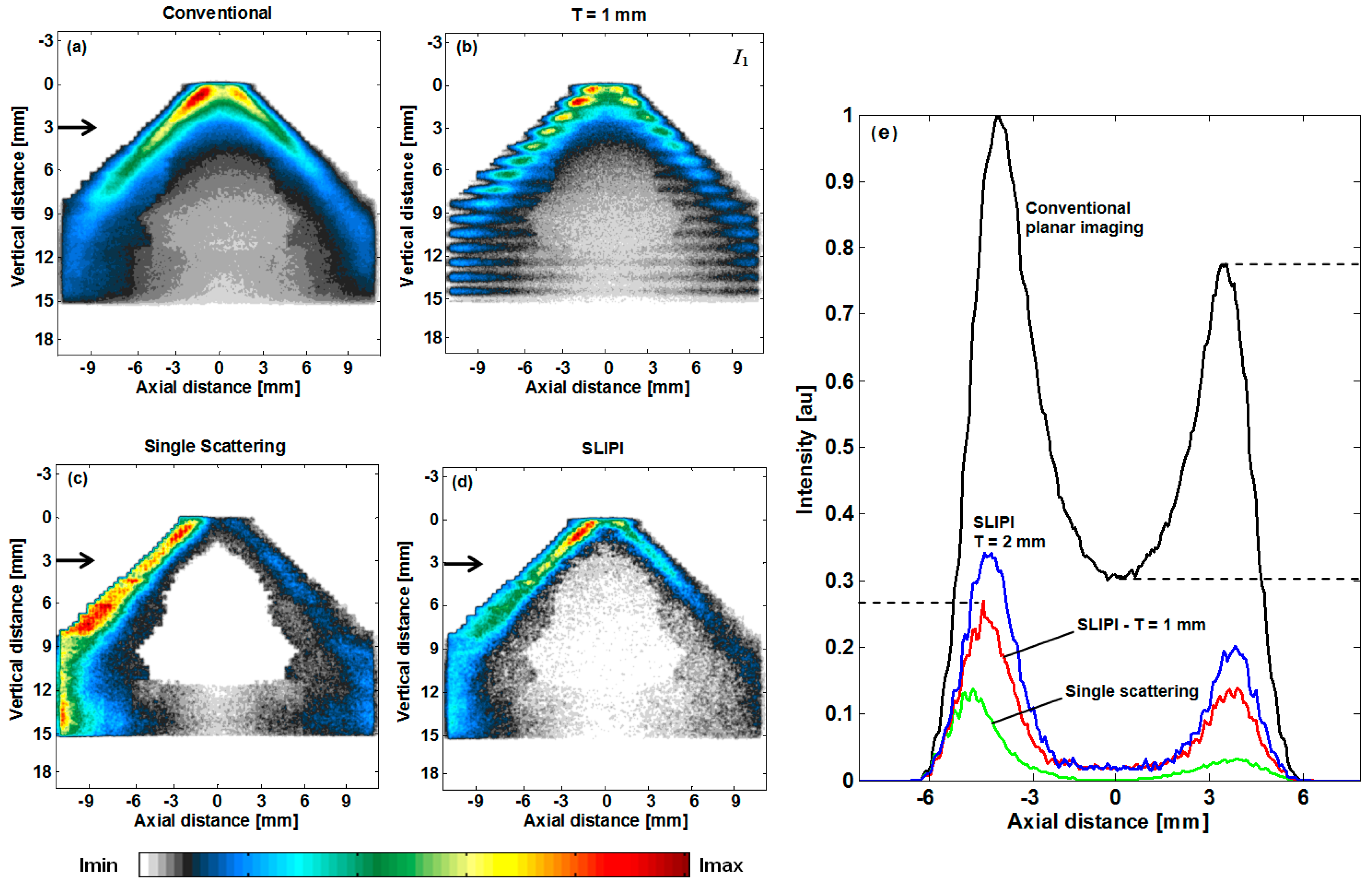
• The fluorescence signal from droplets located in the spray region;
• The Mie scattering signal from droplets located in the spray region;
• The light intensity transmitted through the spray; using a cuvette containing a fluorescing liquid.

The simultaneous recording ensures that the generated images of LIF/Mie signals and transmission imaging are from identical spray operating conditions. This significantly reduces the time it would usually take as compared with two measurements performed sequentially. Furthermore, the same area is viewed on the camera providing the same spatial resolution. Finally, the PDA measurements are utilized for the calibration, and therefore, are not simultaneous with SLIPI-based measurements. Unlike the method to deduce 2D maps of droplets LVF from backlight-illumination based microscopic setup shown in [12], here, PDA calibration and numerical calculations are implemented for LVF calculations. The PDA calibration is preferred over microscopic setup due to its larger dynamic range (smallest droplet diameter measured is up to 3 µm) as compared with the microscopic method (smallest diameter ≥10 µm).

Therefore, this study demonstrates the combination of three optical methods supported by numerical calculations to measure droplets SMD, droplets N, and LVF from the same spray section probed by the laser sheet. The method is extended for intersecting the spray in several 2D layers by means of laser sheet scanning (with a step size of Z = 500 µm). Finally, it is shown that several 2D layers can be combined to generate a 3D map of each individual spray quantity.

2. Description of the Experiment

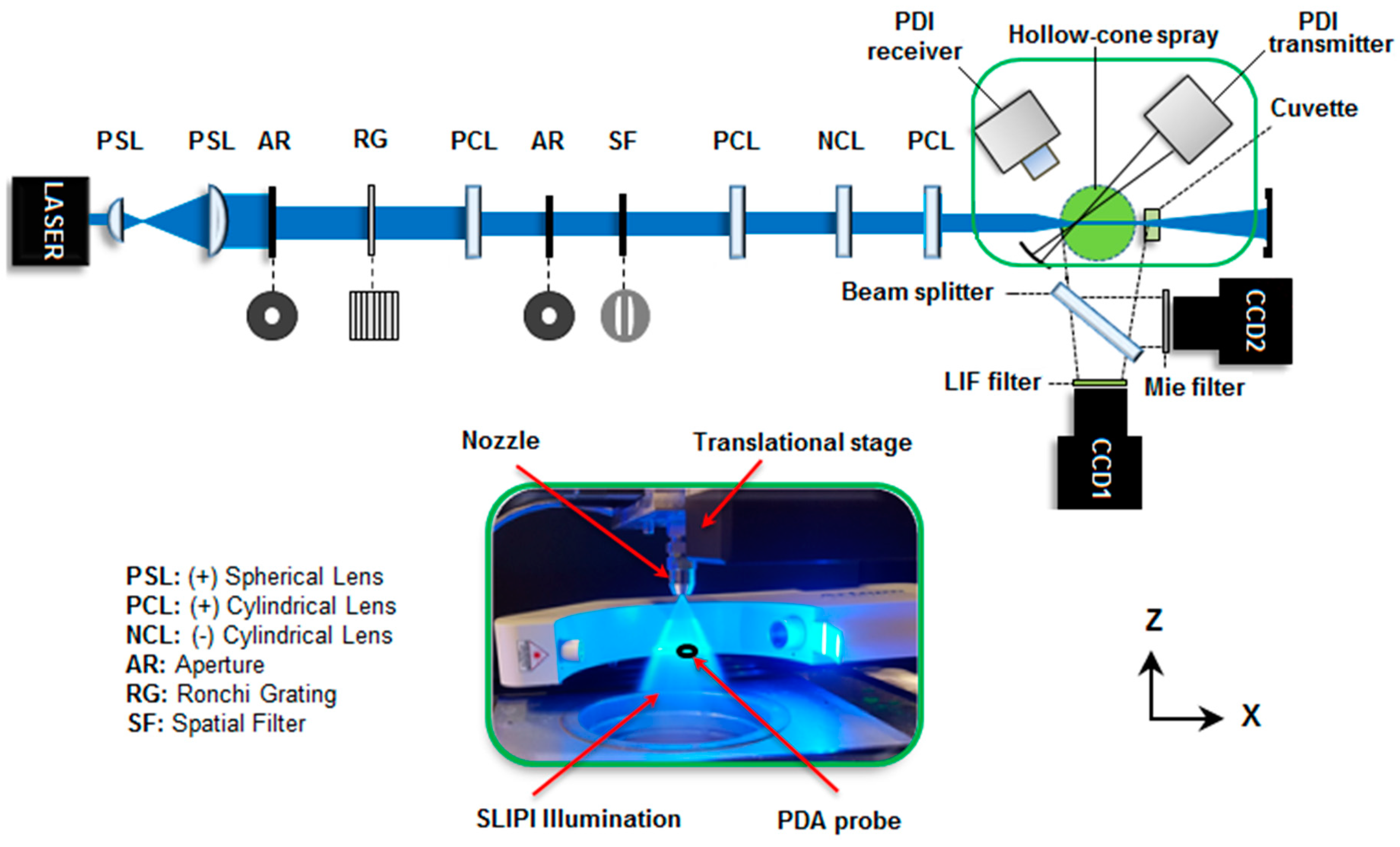
2.1. Combined SLIPI-LIF/Mie and SLIPI-Scan Optical Setup

The schematic of the combined SLIPI-LIF/Mie and SLIPI-scan optical setup is shown in Figure 2. A damaged nozzle of the orifice diameter of 1 mm is used to generate an asymmetric and steady hollow-cone water spray. The liquid is continuously injected at 50 bars injection pressure at room temperature and atmospheric conditions. The defiled nozzle (Order no. 216.324, Lechler Inc., St. Charles, IL, USA) produced completely different droplet size distribution (much larger) and spray pattern (asymmetric) as previously reported with the same nozzle [21]. An asymmetric 3D map of droplets SMD produced with this nozzle is also reported in [23]. In this work, the injected liquid was a solution of water containing fluorescein dye. The dye is excited at 447 nm wavelength using a CW laser (LRD-0447 Series, Laserglow Technologies Inc., Toronto, ON, Canada) producing a broadband LIF signal, which is peaking at 517 nm.

The structured light sheet is generated using the same optical setup as presented in reference [21] and is detailed in Figure 2. The vertically modulated light sheet was around 58 mm in height and approximately 0.25 mm thick. The laser power at the incident wavelength was ~28 mW. A phase Doppler instrument (PDI-TK2 model, Artium Technologies Inc., Sunnyvale, CA, USA) was used, here, for calibration purposes and its measurement probe volume overlapped with the structured light sheet. For the scanning procedure, the spray nozzle was displaced using a translation stage (Standa Ltd., Vilnius, Lithuania) while keeping the illumination and detection systems fixed. The transmission measurements were done using a fluorescing solution contained in glass cuvette located on the laser exit side of the spray. The cuvette and the spray were both contained within the field-of-view of the cameras. A beam splitter was used to simultaneously record the LIF and Mie signals into two identical EM-CCD cameras (Luca R604, Andor Technologies Ltd., Belfast, United Kingdom—1004 × 1002 pixels) denoted as “CCD1” and “CCD2”, respectively, each equipped with individual bandpass filters. The LIF filter was a broadband optical filter centered at 510 nm with 94 nm FWHM (full width at half maximum), while the Mie filter was a narrow-band filter of 447 nm central wavelength with 10 nm FWHM (Edmund Optics Ltd., York, United Kingdom). An identical field-of-view was ensured at a pixel level after calibration using a dotted test pattern. The “CCD1” recorded an image of the LIF signal generated from spray droplets, as well as from the dyed cuvette, while the “CCD2” recorded the Mie signal scattered from the spray droplets only. All images had an exposure time of 0.08 seconds and an accumulation of 20 images was operated for each modulated sub-image corresponding to 60 images, for the 3 sub-images, used for the reconstruction of the SLIPI image. Using SLIPI-scan, the spray was sectioned into a total number of 31 layers (in a “bread slicing” manner), with a step difference of 500 µm corresponding to a depth of 15 mm. The spray was probed at 37 mm below the nozzle tip and on its periphery to ensure the presence of spherical droplets only. Under such conditions, the optical depth (OD) was ~1 only.

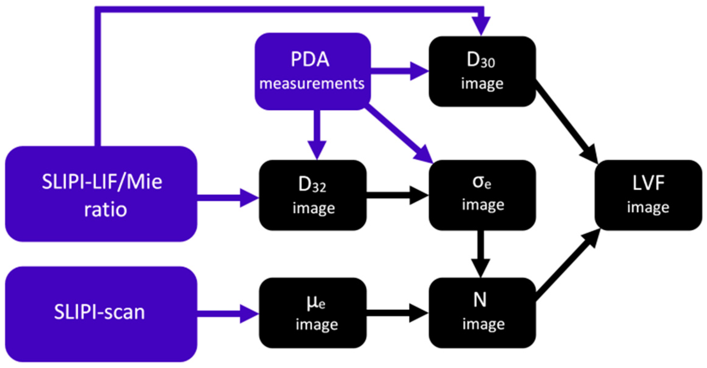
2.2. Process to Extract Scalar Quantities

A flow chart showing the process to extract the spray quantities is given in Figure 3. A general description of the process in steps is as follows:

Step 1 Conversion of SLIPI-LIF/Mie ratio to droplets mean diameters using PDA measurements

The 2D matrix of SLIPI-LIF/Mie ratio is converted to two independent spray quantities, 2D maps of droplets SMD (D₃₂) and droplets volume mean diameter (D₃₀). This is performed according to the calibration between the SLIPI-LIF/Mie ratio and PDA measurements. At a given measurement point, PDA records droplet size distribution, which can be used for the calculation of various mean diameters of droplets, for example, mean diameters D₃₂ and D₃₀ are deduced, here, according to the reference [27].

Step 2 Conversion of SLIPI-LIF/Mie ratio matrix to σ_e maps using PDA data and numerical calculations

As mentioned above, the PDA measurements, performed at a point in the spray, provide the droplet size distribution. Here, the size distribution from PDA is used to calculate the corresponding averaged σ_e (in mm²) according to Lorenz–Mie theory [28]. A Mie calculator developed by the authors, here, based on the algorithm proposed by Bohren and Huffman in [29]. Consequently, each PDA measurement point of size distribution can be converted to averaged σ_e of spray droplets. Therefore, now, the calibrated SLIPI-LIF/Mie ratio matrix (or droplets SMD) is converted to droplet extinction cross-section σ_e.

Step 3 Conversion of SLIPI-LIF/Mie ratio matrix to droplet volume

As previously mentioned, the SLIPI-LIF/Mie ratio is converted to D₃₀ maps using the PDA calibration. Now, the matrix of the volume mean diameter is converted to droplet volume (V) using the formula of volume of a sphere [30].

Step 4 Calculation of droplet local µ_e from SLIPI-scan

The local µ_e of droplets in the spray is calculated using the transmitted light intensity which is recorded from the light fluorescing from a glass cuvette located on the other side of the spray. A light sheet scanning procedure starting from the outside of the spray toward its center is performed. The corrections of light extinction effects over the three-dimensional spray volume lead to the measurement of the local µ_e in mm⁻¹, a technique named SLIPI-scan [25,26]. A detailed description of the SLIPI-scan is given in Section 4.

Step 5 Calculation of droplets N using µ_e and σ_e

To calculate droplets number density (N), two spray quantities, µ_e and σ_e, are required because calculating the ratio µ_e/σ_e, droplets N (#/mm³) can be deduced. The process to calculate µ_e is given in Step 4, while σ_e calculation is discussed in Step 2.

Step 6 Calculation of droplets LVF

Finally, to calculate the LVF of droplets, two quantities, droplets volume (V) and droplets N are required. The LVF is extracted from the pixel-wise multiplication between V and N. The process to deduce droplets V and N is given in Step 3 and Step 5, respectively.

Therefore, using the simultaneously recorded SLIPI-LIF/Mie and SLIPI-scan data in the post-processing described in Figure 3, various scalar quantities of the spray can be calculated. Note that those calculations are made on each pixel of the spray images allowing 2D, as well as 3D mapping of the spray.

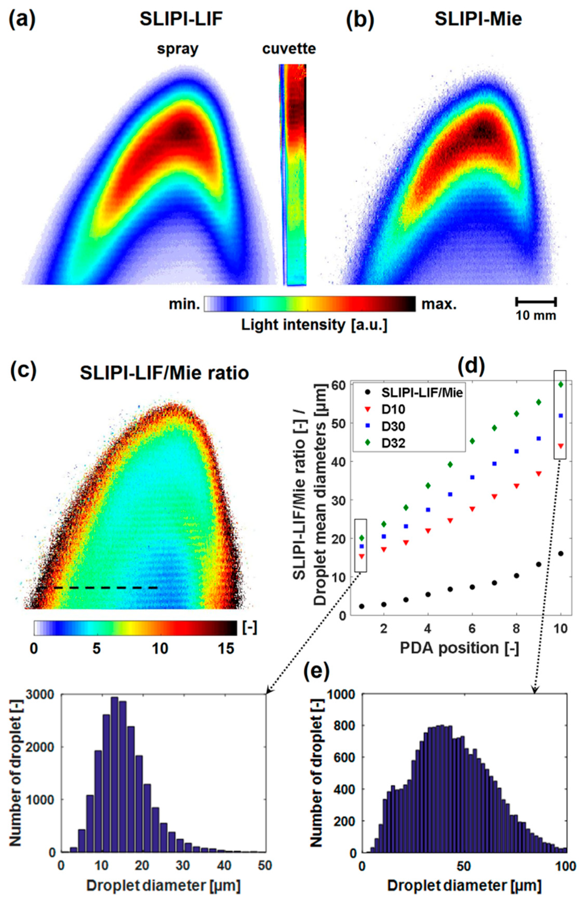
3. SLIPI-LIF/Mie Ratio Method for Droplet SMD and Extinction Cross-Section (σ_e) Mapping

3.1. Description of LIF/Mie Droplet Sizing

The SMD of an ensemble of the spherical droplets in sprays can be calculated from the ratio of their LIF/Mie optical signals simultaneously measured from the same probe location [11,24,31]. The method assumes that the fluorescence from the liquid phase, $I_{LIF}$, is proportional to the droplet volume, $d^3$, and the Mie scattered light intensity, $I_{Mie}$, from the same droplet is proportional to its surface, $d^2$, [32,33,34]. Apart from this assumption, three important conditions must be respected. First, the technique is only valid for spherical droplets and it does not withstand for non-spherical liquid structures and ligaments [24,31]. Second, the fluorescence from the gas phase must be excluded [35]. Third, all photons reaching the camera should have experienced only one scattering event prior to detection [16]. If those conditions are respected, the resulting intensity ratio, $R_{LIF/Mie}$, is then proportional to SMD of droplets as:

$$R_{LIF/Mie}=\frac{I_{LIF}}{I_{Mie}}=\frac{K_{LIF}}{K_{Mie}}·\frac{{{\displaystyle \sum }}_{i=0}^n{N}_i·d_i^3}{{{\displaystyle \sum }}_{i=0}^n{N}_i·d_i^2}=K·SMD$$

(3)

where $K_{LIF}$ and $K_{Mie}$ are coefficients related to dye concentration, laser power, signal collection angle, detector response, and scattering efficiency, etc. Here $K$ defines the calibration curve which is equal to the ratio $K_{LIF}/K_{Mie}$. The calibration curve can be either deduced by using the calibration of LIF/Mie ratio with the absolute SMD measured by the PDA system [21,22] or calibrating the ratio by means of monodisperse droplet generated by a droplet generator [24,36].

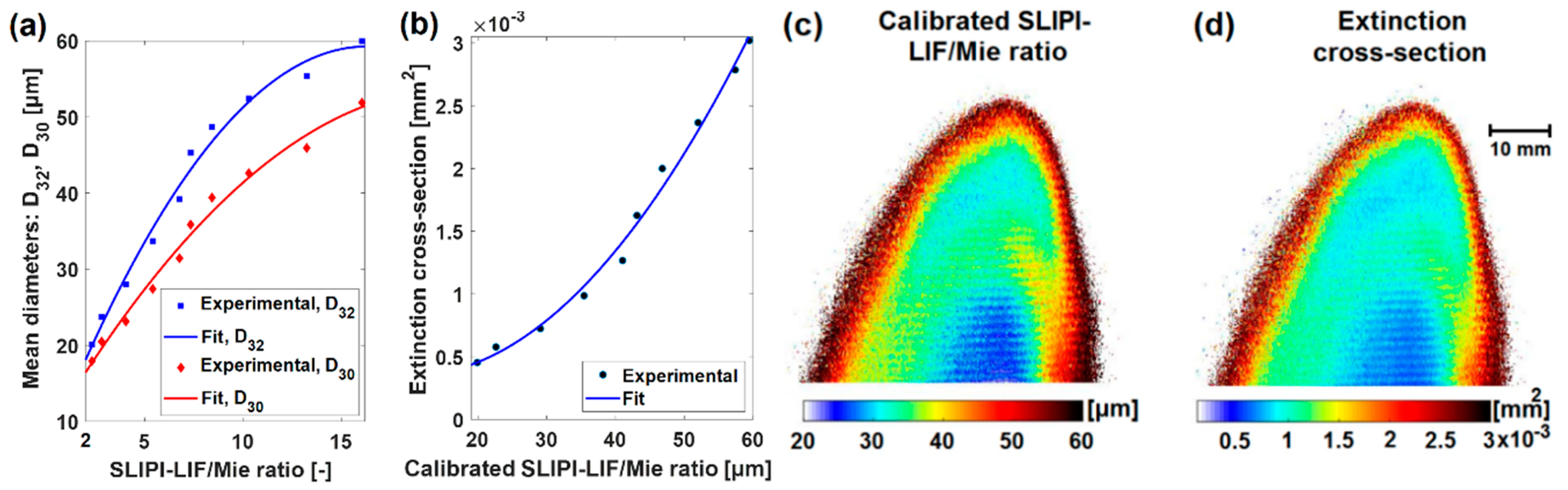
3.2. Calibration of SLIPI-LIF/Mie Ratio and Extinction Cross-Section (σ_e) Images

Figure 4 is an example of results at layer number m = 30 which corresponds to the depth position Z = 15 mm. In (a) the SLIPI-LIF image of the spray is shown together with the transmitted light from the fluorescing liquid in the cuvette. The Mie image and the intensity ratio, SLIPI-LIF/Mie are given in (b) and (c), respectively. These images are recorded using the experiments described in Section 2.1. Some residual stripes are seen on the processed SLIPI images. These artifacts can be reduced by averaging the data over a larger number of images, effectively reducing the intensity variations between the three sub-images. Other reasons for their occurrence are given in [16,20] together with some suppression strategy.

The black dashed line in Figure 4c corresponds to the location where PDA measurements are performed. For each location, 20,000 validated droplet size measurements are recorded by the PDA instrument. In all measurements, the percentage of validation rate was above 96%, confirming a good sphericity of the droplets at a distance 7.5 cm below the nozzle tip without unwanted multi-occupancy effects. Figure 4d shows the SLIPI-LIF/Mie ratio and various mean diameters, D₁₀, D₃₀, and D₃₂ plotted against the PDA measurement position. Those mean diameters are calculated by using the droplet distribution histogram shown in Figure 4e for measurement positions X = 1 and X = 10. From mean diameters, it is seen that arithmetic mean diameter (D₁₀) is the lowest mean diameter while SMD, D₃₂, is the largest. The size distribution histograms are shown in Figure 4e or a similar distribution can also be utilized for deducing several other mean diameters, as given in reference [13,27].

Figure 5a shows the plots of SLIPI-LIF/Mie ratio against droplets D₃₂ and D₃₀. Both the experimental data and the calibration fit for correlating the ratio with mean diameters are seen. In a recent study, Corber et al. [37] extensively investigated the SLIPI-LIF/Mie ratio and the PDA calibration in a simple pressure atomizer. A calibration curve similar to Figure 5a in this study is also reported by the authors in [37]. Figure 5b shows the plot of calibrated SLIPI-ratio (droplets SMD) against the corresponding droplets σ_e. To deduce the averaged σ_e, the histogram of the droplets size distribution (see Figure 4e) for each measured SMD value is used as input data to the Lorenz–Mie calculator software developed by the authors. The input incident wavelength is set, here, to 447 nm, while the refractive indices are set to 1 for air and 1.33 for the water droplets. The entire medium is assumed to be non-absorbing. Figure 5c shows the calibrated SLIPI-LIF/Mie ratio maps representing droplet SMD extracted using the calibration curve given in Figure 5a, while Figure 5d shows the droplets σ_e maps obtained from the calibration curve shown in Figure 5b. It is observed in Figure 5c that the largest droplets corresponding to approximately SMD = 60 µm are located at the spray edge, while the smallest droplets of approximately SMD = 25 µm are in the spray center. It is seen in Figure 5d that the σ_e varies from 0.5 × 10⁻³ mm² in the center of the spray to 3 × 10⁻³ mm² at the outermost edges of the spray.

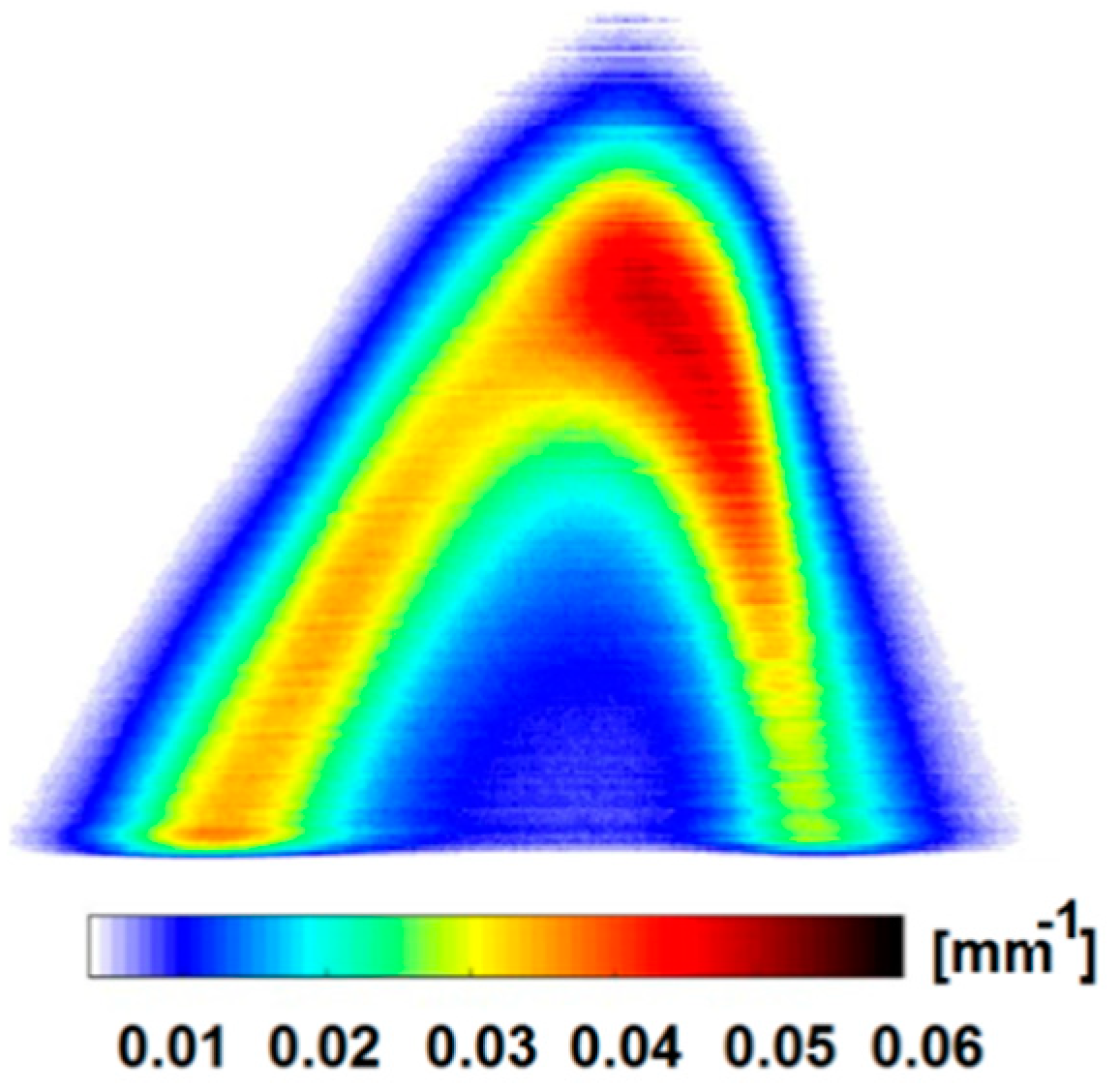
4. SLIPI-Scan for Extinction Coefficient (µ_e) Mapping

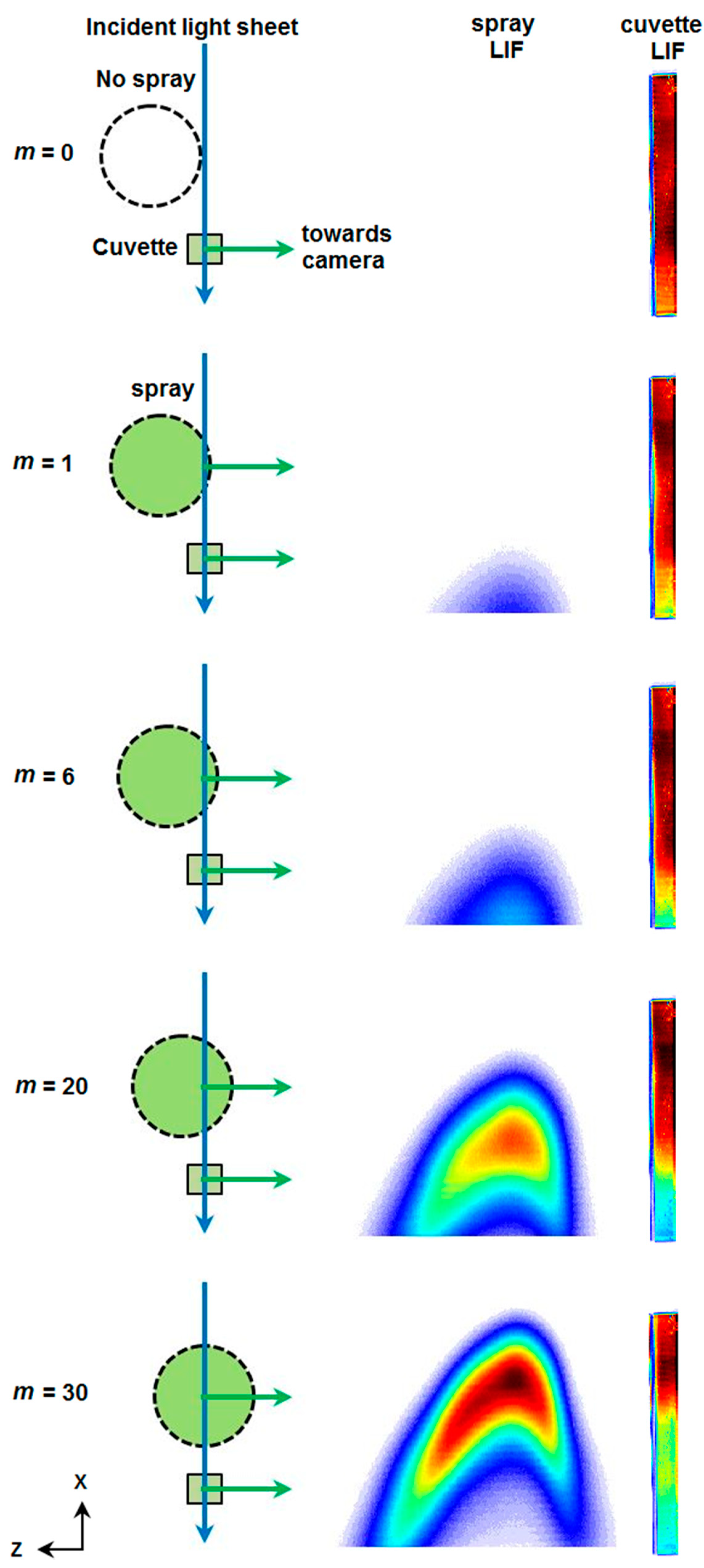
4.1. Description of the SLIPI-Scan Technique

The SLIPI-scan technique is used to extract the µ_e by imaging the sample in a “bread slicing” manner by means of a laser sheet with sinusoidal intensity modulation (see Section 2.1). For each slice (layer), three sub-images with a 120° phase shift are acquired and the corresponding SLIPI image is constructed according to Equation (2). In order to correct for the light extinction between the laser sheet and the camera, also known as signal attenuation, a scanning procedure starting from the outside of the spray towards its center is performed [25,26]. By stepwise acquisition of SLIPI images at different depths in the sample, one obtains a stack of 2D SLIPI images taken at different planes (m) of the sample, as is illustrated in a top view in Figure 6. At plane m = 0, i.e., before the introduction of the spray, the light sheet is incident on the reference cuvette only. The amount of fluorescence signal emitted towards the camera by the reference solution is captured in the first image of the stack. The acquired image at this plane m = 0 serves as a reference to measure the intensity incident on the spray for all subsequent planes. At plane m = 1, the lower part of the laser sheet is incident on the outermost edge of the spray. In the corresponding SLIPI image, both fluorescence signals from the edge of the spray, as well as from the reference cuvette, are now being detected. One notices that the recorded intensity from the reference cuvette has decreased at the bottom part at a height corresponding to the height where the laser sheet interacts with the spray. Following this manner, the spray is scanned in a total of 31 planes, separated by 500 μm each, until the middle of the spray is reached.

4.2. SLIPI-Scan Realization in Sprays

The recorded stack of 2D-SLIPI images (see Figure 6) can be described as a 3D matrix of voxels defined by the number of pixels in the X- and Y-direction and the number of planes, m, in the Z-direction. Along with any row $l$ through the spray in a given plane m, the irradiance $I$ follows the Beer–Lambert’s law:

$$I\left(k+1,l,m\right)=I\left(k,l,m\right)e^{-{\mu }_e\left(k,l,m\right)dx}$$

(4)

where $k$ denotes the column and $dx$ its corresponding width in the image. For the first column in each plane, incident irradiance is determined from the reference image at plane m = 0. Alternatively, the irradiance in each voxel in the spray can be expressed as the difference between the incident irradiance in the previous voxel along the direction of propagation and the irradiance lost through scattering (or LIF in this case) $I_s$ in that previous voxel:

$$I\left(k+1,l,m\right)=I\left(k,l,m\right)-I_s\left(k,l,m\right)$$

(5)

The combination of Equations (4) and (5) yields:

$${\mu }_e\left(k,l,m\right)=-ln\left(\frac{(I\left(k,l,m\right)-I_s\left(k,l,m\right)}{I\left(k,l,m\right)}\right)\frac{1}{dx}$$

(6)

The scattered irradiance, $I_s$, is calculated as given in references [25,26]:

$$I_s\left(k,l,m\right)=\frac{S\left(k,l,m\right)\left(I_i\left(l,m\right)-I_f\left(l,m\right)\right)}{\left(1-a\left(k,l,m\right)\right){{\displaystyle \sum }}_{k=1}^{k_{max}}\frac{S\left(k,l,m\right)}{\left(1-a\left(k,l,m\right)\right)}}$$

(7)

where $S$ is the detected SLIPI signal in the images; $I_i$ and $I_f$ are the incident and final irradiance obtained from the images of the reference cuvette at plane m = 0 and the corresponding plane m, respectively; and $a$ describes the signal attenuation that signal, from a particular voxel $\left(k,l,m\right)$, experiences on its way to the camera. It is calculated as:

$$a\left(k,l,m\right)=1-exp\left(-{\displaystyle \sum }_{m^{\prime }}^{m-1}{\mu }_e\left(k,l,m^{\prime }\right)dz\right)$$

(8)

For the calculation of $I_s\left(k,l,1\right)$, it is assumed that the signal attenuation is negligible for that plane, i.e., $a\left(k,l,1\right)=0$ For the calculation of $I_s\left(k,l,1\right)$, it is assumed that the signal attenuation is negligible for that plane, i.e., $a\left(k,l,1\right)=0$ [25,26]. Hence, all parameters in Equation (7) are available and the extinction coefficient can be calculated according to Equation (6) for the first plane of the sample. Then, the μ_e determined in the first plane is used to calculate the signal attenuation $a\left(k,l,2\right)$ in the second plane. From there, $I_s\left(k,l,2\right)$ can be calculated according to Equation (7), which in return allows calculation of ${\mu }_e\left(k,l,2\right)$ according to Equation (6). Continuing this iterative process in a plane-wise manner allows the calculation of μ_e for all planes of the spray imaged. Figure 7 shows the resulting 2D image of local μ_e deduced at plane m = 30 (Z = 15 mm).

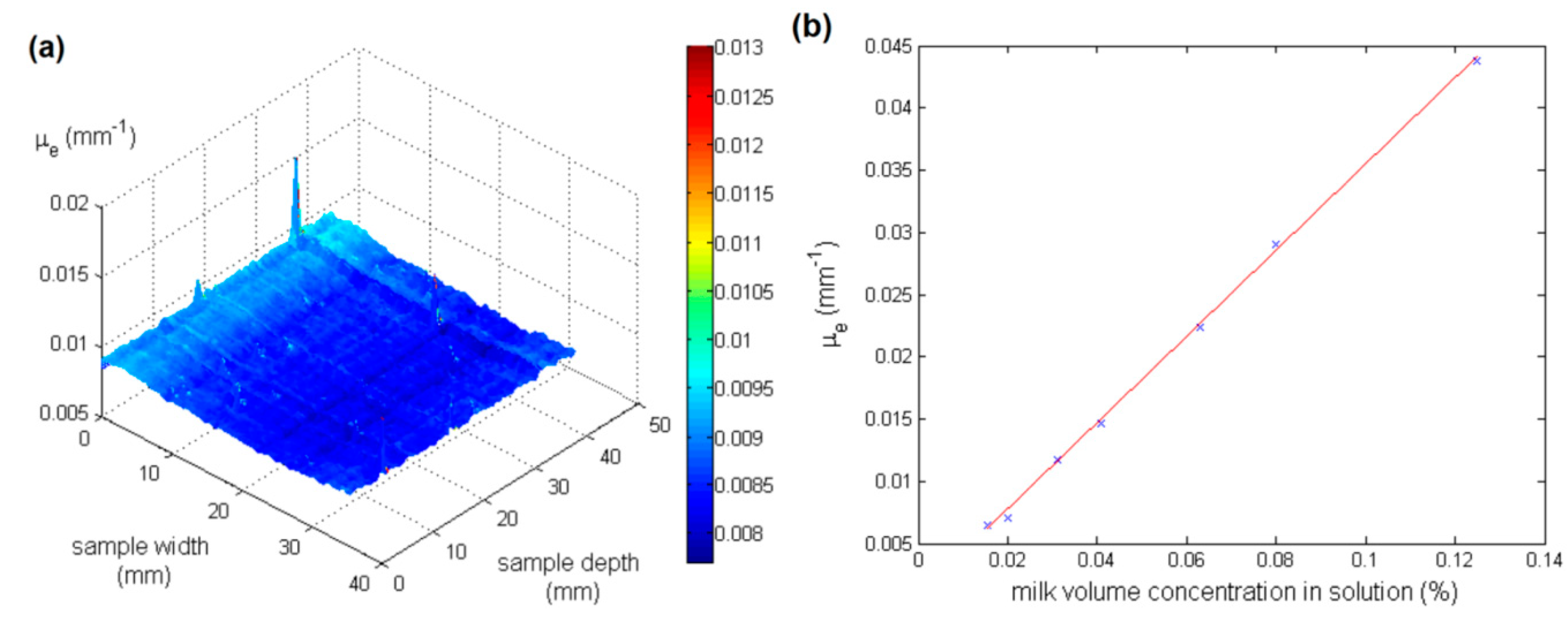
4.3. Verifiaction of SLIPI-Scan Algorithm on a Homogeneous Medium

The SLIPI-scan approach algorithm has been verified previously and the details of the experiment can be found in [25,26]. Figure 8 shows the example of SLIPI-scan measurement on the diluted homogeneous milk samples (adapted from [26])). In Figure 8a, a fairly constant extinction coefficient, as expected, of 0.0085 mm⁻¹ is measured. The few noticeable spikes were attributed to signal distortion from scratches or dirt on the container surface. In Figure 8b, several diluted milk solutions (in %) were used to measure the extinction coefficient at various milk concentration. It is seen that the measured extinction coefficient remains linear with the milk concentration, as expected. These observations confirm the reliable 3D estimation of the extinction coefficient when using SLIPI-scan.

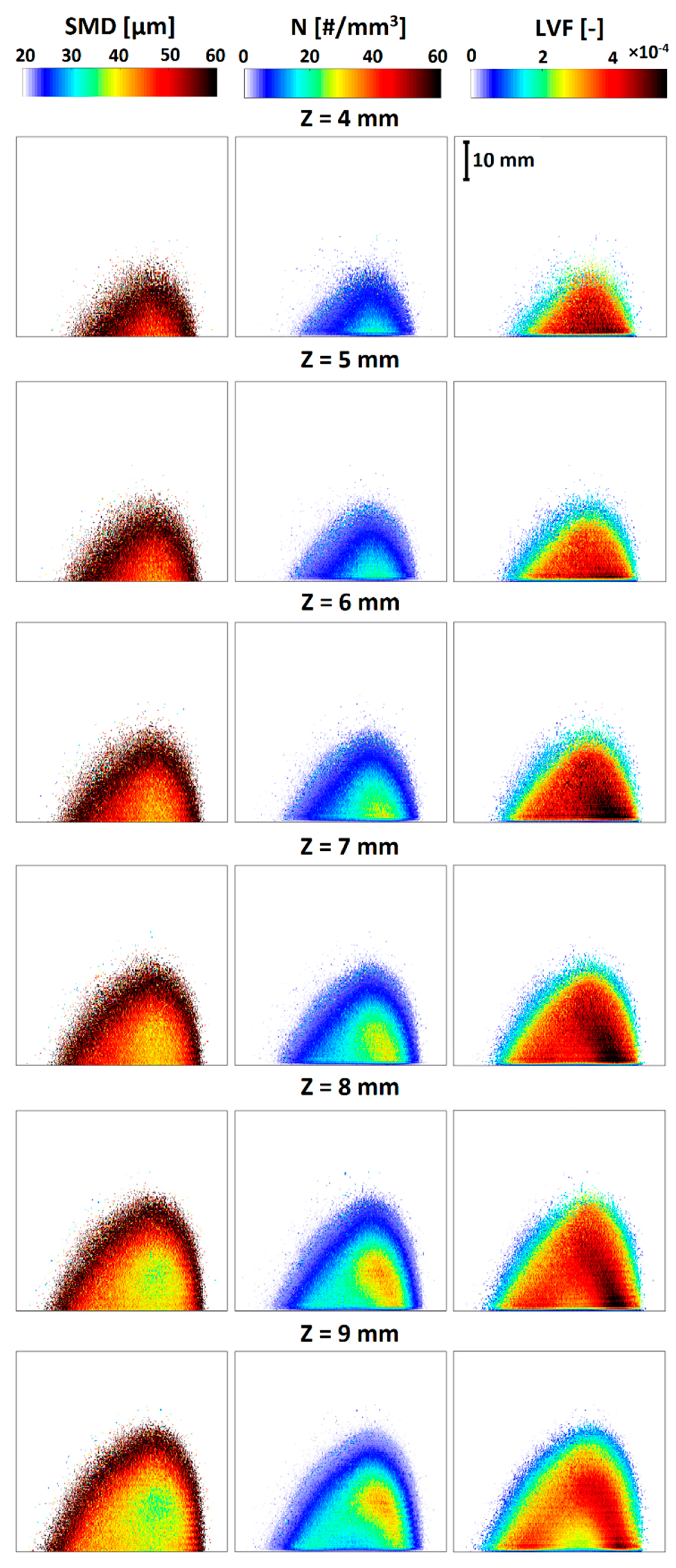
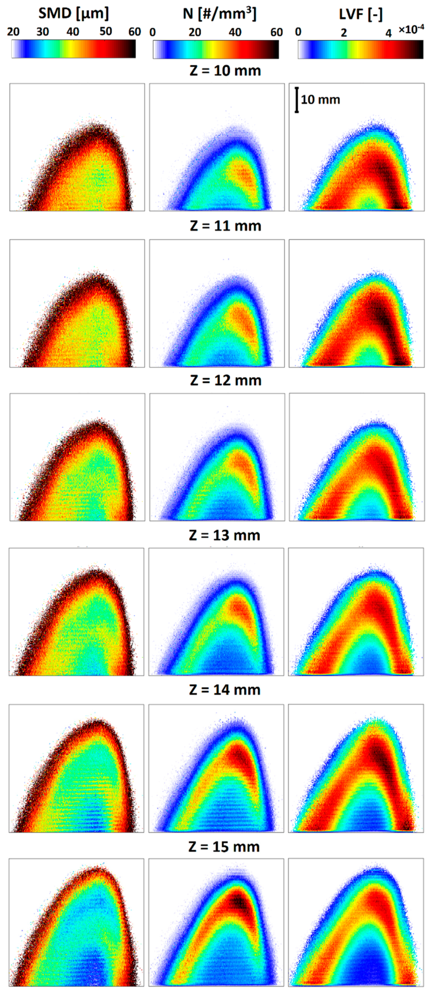
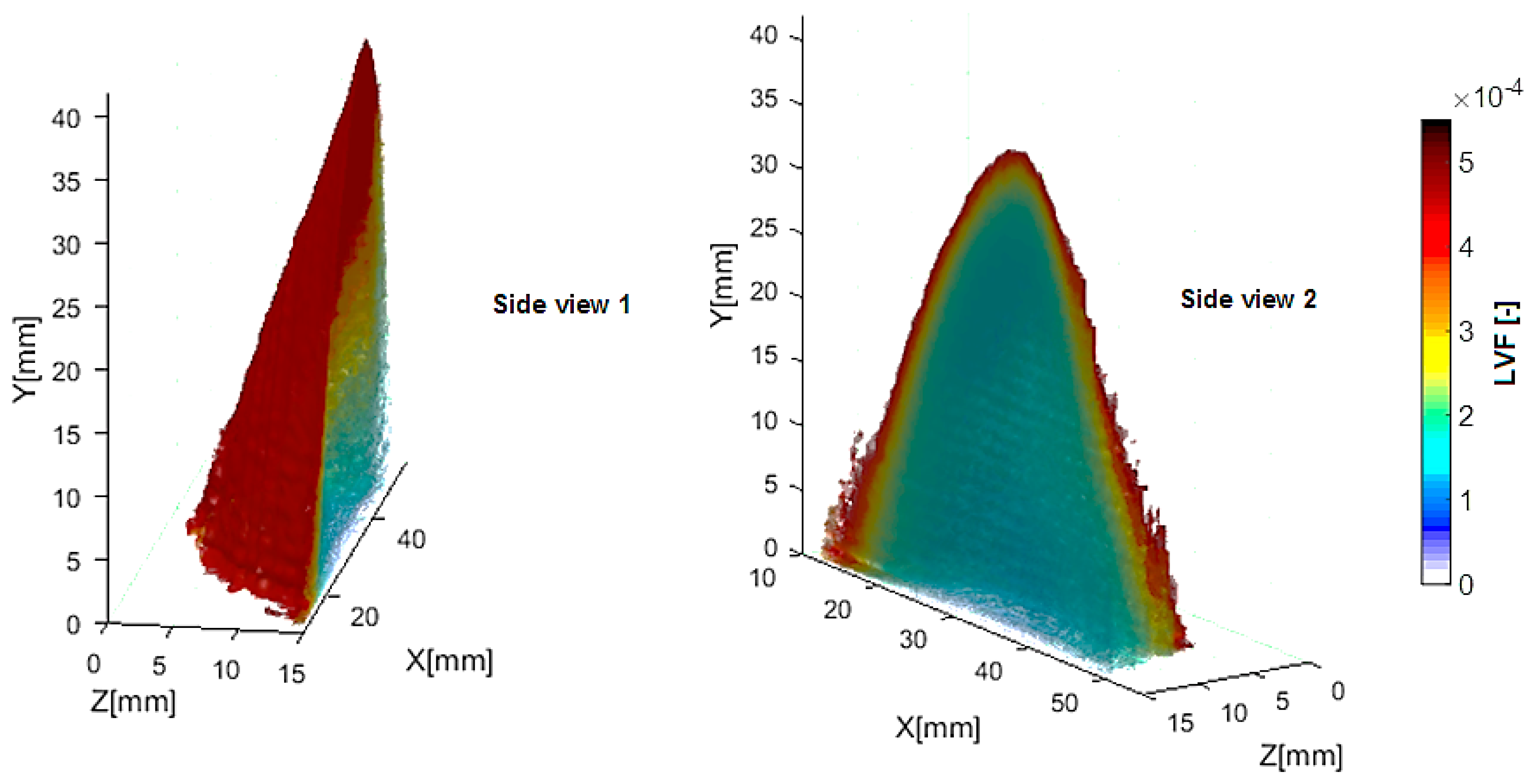
5. 2D Results of Droplet SMD, Number Density, and Liquid Volume Fraction

Figure 9 and Figure 10 show the 2D images of the spray quantities, i.e., droplet SMD, droplet concentration (N) and liquid volume fraction (LVF) for spray sections at Z = 4 mm to 9 mm and at Z = 10 mm to Z = 15 mm, respectively, as follows:

• At Z = 4 mm, droplet SMD ranges between 50 µm to 60 µm, N value ranges from 5 to 20 droplets per mm³, LVF ranges between 2.5 × 10⁻⁴ to 5.5 × 10⁻⁴;
• At Z = 8 mm, droplet SMD ranges from a minimum value of 35 µm to a maximum value of 60 µm, N value ranges from 5 to 35 droplets per mm³, LVF ranges between 1.8 × 10⁻⁴ to 5.5 × 10⁻⁴;
• At Z = 12 mm, droplet SMD ranges from 30 to 60 µm, N value ranges from a minimum of 5 droplets per mm³ to a maximum of 40 droplets per mm³, LVF ranges between 1 × 10⁻⁴ to 5.5 × 10⁻⁴;
• At Z = 15 mm, droplet SMD ranges from 20 to 60 µm, N from 5 to 60 droplets per mm³, LVF ranges from 0.1 × 10⁻⁴ to 5.5 × 10⁻⁴.

The absolute SMD values measured with the presented approach follows well with the PDA data, as has been previously demonstrated in [21], with the calibrated SLIPI-LIF/Mie ratio and SMD acquired from PDA for the hollow-cone spray of OD ~1. The extracted N and LVF values in this investigation are in the order of the theoretical calculations performed based on a homogeneous distribution of monodisperse non-absorbing dielectric spherical droplets in reference [5]. Note that the numerical calculations in [5] are verified by an experimental study performed by Berrocal et al. in [38]. Using all 30 sections (15 mm depth) of 2D maps of LVF (see Figure 9 and Figure 10), a resultant 3D reconstruction can be generated as shown in Figure 11. The LVF value is lowest at the center of the spray and highest at the spray peripheries.

6. Conclusions

In conclusion, the light sheet scanning approach based on structured illumination, proposed here, provides a series of 2D images where most scalar quantities from the spray region are extracted. The 2D images obtained at several Z-distances can be combined to reconstruct a 3D map of the scalar quantities. This proof-of-concept work is promising for future complete characterization of optically dense sprays over large spray volumes. It should, however, be pointed out that further work is needed to investigate the measurement accuracy and precision of the approach. The validation and accuracy of results presented in Section 5 depend largely on the basis of reliable qualitative data extracted as SLIPI-LIF/Mie ratio (for droplet SMD mapping) and SLIPI-scan light transmission measurements (for the determination of extinction coefficient). Finally, as the technique relies on spherical droplets, it is important to emphasis that it should not be employed near the nozzle tip, due to the presence of irregular liquid bodies and ligaments in this region where the spray is being formed.

References

1. Chigier, N. An assessment of spray technology - Editorial. At. Sprays 1993, 3, 365–371. [Google Scholar] [CrossRef]
2. Ashgriz, N. Handbook of Atomization and Sprays: Theory and Applications; Springer: Boston, MA, USA, 2011. [Google Scholar]
3. Lefebvre, A.; McDonell, V. Atomization and Sprays, 2nd ed.; CRC Press: Boca Raton, FL, USA, 2017. [Google Scholar]
4. Lee, K.; Abraham, J. Spray Applications in Internal Combustion Engines. In Handbook of Atomization and Sprays: Theory and Applications; Ashgriz, N., Ed.; Springer: Boston, MA, USA, 2011. [Google Scholar]
5. Fansler, T.D.; Parrish, S.E. Spray measurement technology: A review. Meas. Sci. Technol. 2015, 26. [Google Scholar] [CrossRef]
6. Bachalo, W. Spray diagnostics for the twenty-first century. At. Sprays 2000, 10, 439–474. [Google Scholar] [CrossRef]
7. Mishra, Y.N.; Koegl, M.; Baderschneider, K.; Hofbeck, B.; Berrocal, E.; Conrad, C.; Will, S.; Zigan, L. 3D mapping of droplet Sauter mean diameter in sprays. Appl. Opt. 2019, 58, 3775–3783. [Google Scholar] [CrossRef]
8. Pastor, J.V.; López, J.J.; Enrique Juliá, J.; Benajes, J.V. Planar Laser-Induced Fluorescence fuel concentration measurements in isothermal Diesel sprays. Opt. Express. 2002, 10, 309–323. [Google Scholar] [CrossRef]
9. Westerweel, J.; Elsinga, G.E.; Adrian, R.J. Particle Image Velocimetry for Complex and Turbulent Flows. Annu. Rev. Fluid Mech. 2013, 45, 409–436. [Google Scholar] [CrossRef]
10. Fansler, T.D.; Drake, M.C.; Gajdeczko, B.; Düwel, I.; Koban, W.; Zimmermann, F.P.; Schulz, C. Quantitative liquid and vapor distribution measurements in evaporating fuel sprays using laser-induced exciplex fluorescence. Meas. Sci. Technol. 2009, 20, 125401. [Google Scholar] [CrossRef]
11. Yeh, C.-N.; Kosaka, H.; Kamimoto, T. Fluorescence/scattering image technique for particle sizing in unsteady diesel spray. Trans. Jpn. Soc. Mech. Eng. Ser. B 1993, 59, 4008–4013. [Google Scholar] [CrossRef] [Green Version]
12. Deshmukh, D.; Ravikrishna, R.V. A method for measurement of planar liquid volume fraction in dense sprays. Exp. Therm. Fluid Sci. 2013, 46, 254–258. [Google Scholar] [CrossRef]
13. Mishra, Y.N. Droplet Size, Concentration, and Temperature Mapping in Sprays Using SLIPI-based Techniques. Ph.D. Thesis, Lund University, Lund, Sweden, 2018. [Google Scholar]
14. Brown, C.T.; Mcdonnell, V.G.; Talley, D.G. Accounting for laser extinction, signal attenuation, and secondary emission while performing optical patternation in a single plane. In Proceedings of the ILASS Americas 2002 15th Annual Conference on Liquid Atomization and Spray Systems, Madison, WI, USA, 14–17 May 2020. [Google Scholar]
15. Berrocal, E. Multiple Scattering of Light in Optical Diagnostics of Dense Sprays and Other Complex Turbid Media. Ph.D. Thesis, Cranfield University, Bedford, UK, 2006. [Google Scholar]
16. Kristensson, E. Structured Laser Illumination Planar Imaging SLIPI Applications for Spray Diagnostics. Ph.D. Thesis, Lund University, Lund, Sweden, 2012. [Google Scholar]
17. Berrocal, E.; Kristensson, E.; Richter, M.; Linne, M.; Aldén, M. Application of structured illumination for multiple scattering suppression in planar laser imaging of dense sprays. Opt. Express. 2008, 16, 17870–17881. [Google Scholar] [CrossRef] [PubMed] [Green Version]
18. Kristensson, E.; Berrocal, E.; Richter, M.; Pettersson, S.G.; Aldén, M. High-speed structured planar laser illumination for contrast improvement of two-phase flow images. Opt. Lett. 2008, 33, 2752–2754. [Google Scholar] [CrossRef] [PubMed] [Green Version]
19. Berrocal, E.; Kristensson, E.; Sedarsky, D.; Linne, M. Analysis of the SLIPI technique for multiple scattering suppression in planar imaging of fuel sprays. In Proceedings of the ICLASS 2009, 11th Triennial International Annual Conference on Liquid Atomization and Spray Systems, Vail, CO, USA, 26–30 July 2009. [Google Scholar]
20. Mishra, Y.N.; Kristensson, E.; Koegl, M.; Jönsson, J.; Zigan, L.; Berrocal, E. Comparison between two-phase and one-phase SLIPI for instantaneous imaging of transient sprays. Exp. Fluids 2017, 58. [Google Scholar] [CrossRef] [Green Version]
21. Mishra, Y.N.; Kristensson, E.; Berrocal, E. Reliable LIF/Mie droplet sizing in sprays using structured laser illumination planar imaging. Opt. Express. 2014, 22, 4480–4492. [Google Scholar] [CrossRef] [PubMed]
22. Kulkarni, A.P.; Chaudhari, V.D.; Bhadange, S.R.; Deshmukh, D. Planar drop-sizing and liquid volume fraction measurements of airblast spray in cross-flow using SLIPI-based techniques. Int. J. Heat Fluid Flow 2019, 80. [Google Scholar] [CrossRef]
23. Mishra, Y.N.; Kristensson, E.; Berrocal, E. 3D droplet sizing and 2D optical depth measurements in sprays using SLIPI based techniques. In Proceedings of the 18th International Symposium on the Application of Laser and Imaging Techniques to Fluid Mechanics, Lisbon, Portugal, 4–7 July 2016. [Google Scholar]
24. Koegl, M.; Hofbeck, B.; Baderschneider, K.; Mishra, Y.N.; Huber, F.J.T.; Berrocal, E.; Will, S.; Zigan, L. Analysis of LIF and Mie signals from single micrometric droplets for instantaneous droplet sizing in sprays. Opt. Express 2018, 26, 31750–31766. [Google Scholar] [CrossRef] [PubMed]
25. Wellander, R.; Berrocal, E.; Kristensson, E.; Richter, M.; Aldén, M. Three-dimensional measurement of the local extinction coefficient in a dense spray. Meas. Sci. Technol. 2011, 22, 125303. [Google Scholar] [CrossRef]
26. Tscharntke, T. Development of a New Dosimetry Technique. Master’s Thesis, Lund University, Lund, Sweden, 2015. [Google Scholar]
27. Mugele, R.A.; Evans, H.D. Droplet Size Distribution in Sprays. Ind. Eng. Chem. 1951, 43, 1317–1324. [Google Scholar] [CrossRef]
28. van de Hulst, H.C. Light Scattering by Small Particles; John Wiley & Sons: New York, NY, USA, 1957. [Google Scholar]
29. Bohren, C.F.; Huffman, D.R. Appendixes: Computer Programs. In Absorption and Scattering of Light by Small Particles; Wiley-VCH Verlag GmbH: Weinheim, Germany, 2007. [Google Scholar]
30. Akafuah, N.K.; Salazar, A.J.; Saito, K. Estimation of liquid volume fraction and droplet number density in automotive paint spray using infrared thermography-based visulaization technique. At. Sprays 2009, 19, 847–861. [Google Scholar] [CrossRef]
31. Domann, R.; Hardalupas, Y. Quantitative Measurement of Planar Droplet Sauter Mean Diameter in Sprays using Planar Droplet Sizing. Part. Part. Syst. Charact. 2003, 20, 209–218. [Google Scholar] [CrossRef]
32. Le Gal, P.; Farrugia, N.; Greenhalgh, D.A. Laser Sheet Dropsizing of dense sprays. Opt. Laser Technol. 1999, 31, 75–83. [Google Scholar] [CrossRef]
33. Frackowiak, B.; Tropea, C. Numerical analysis of diameter influence on droplet fluorescence. Appl. Opt. 2010, 49, 2363–2370. [Google Scholar] [CrossRef] [PubMed]
34. Koegl, M.; Baderschneider, K.; Bauer, F.J.; Hofbeck, B.; Berrocal, E.; Will, S.; Zigan, L. Analysis of the LIF/Mie Ratio from Individual Droplets for Planar Droplet Sizing: Application to Gasoline Fuels and. Their Mixtures with Ethanol. Appl. Sci. 2019, 9, 4900. [Google Scholar] [CrossRef] [Green Version]
35. Zeng, W.; Xu, M.; Zhang, Y.; Wang, Z. Laser sheet dropsizing of evaporating sprays using simultaneous LIEF/MIE techniques. Proc. Combust. Inst. 2013, 34, 1677–1685. [Google Scholar] [CrossRef]
36. Park, S.; Cho, H.; Yoon, I.; Min, K. Measurement of droplet size distribution of gasoline direct injection spray by droplet generator and planar image technique. Meas. Sci. Technol. 2002, 13, 859. [Google Scholar] [CrossRef]
37. Corber, A.; Vena, P.; Chishty, W. Uncertainty Assessment of Calibrated Structured Planar LIF/Mie Ratio-metric Imaging. In Proceedings of the 29th Conference on Liquid Atomization and Spray Systems, ILASS-Europe, Paris, France, 2–4 September 2019. [Google Scholar]
38. Berrocal, E.; Kristensson, E.; Hottenbach, P.; Aldén, M.; Grünefeld, G. Quantitative imaging of a non-combusting diesel spray using structured laser illumination planar imaging. Appl. Phys. B 2012, 109, 683–694. [Google Scholar] [CrossRef]
Figure 1. Monte Carlo simulation results from [19] showing a comparison between conventional planar Mie imaging and structured laser illumination planar imaging (SLIPI) for a simulated hollow-cone spray. (a) The conventional image; (b) the modulated light sheet of T = 1 mm period; (c) the single light scattering; and (d) the SLIPI images; (e) the intensity profiles along the horizontal axis, at 3 mm below the spray orifice. It is observed from the SLIPI image that most of the multiple light scattering is suppressed and that smaller modulation patterns are more efficient in suppressing effects from multiple light scattering.
Applsci 10 01369 g001
Figure 2. Optical setup of the combined SLIPI laser-induced fluorescence/Mie scattering (SLIPI-LIF/Mie) ratio and SLIPI-scan method. The illumination section (in the green box) consists of a translation stage, spray nozzle, SLIPI illumination, and phase Doppler anemometry (PDA) probe volume. The optical signal detection section consists of a beam splitter, LIF and Mie optical filters, and two identical EM-CCD cameras.
Applsci 10 01369 g002
Figure 3. Simplified flowchart of the image post-processing for extracting several important spray scalar quantities such as the droplets Sauter mean diameter (SMD), the droplets number density (N), and the liquid volume fraction (LVF). The process is performed after recording spay images via a scanning procedure where the SLIPI-LIF signal, the SLIPI-Mie signal, and the light intensity transmitted through the spray are simultaneously recorded.
Applsci 10 01369 g003
Figure 4. (a) SLIPI-LIF image of the spray and the dye cuvette; (b) SLIPI-Mie image; (c) SLIPI-LIF/Mie ratio image of the spray; the PDA measurements are plotted in (d) against the SLIPI-LIF/Mie ratio and droplet mean diameters; (e) histograms of droplet size distributions measured using PDA.
Applsci 10 01369 g004
Figure 5. (a) The calibration curve of the SLIPI-LIF/Mie ratio plotted against droplet mean diameters, D32 and D30. Both experimental data and calibration fit are given; (b) the calibration curve for the calibrated SLIPI-LIF/Mie ratio (SMD or D32) plotted against droplet extinction cross-section. The droplet extinction cross-section is deduced from the Lorenz–Mie theory using the droplet size distribution histograms given in Figure 4e; (c) the calibrated SLIPI-LIF/Mie ratio showing the droplet SMD (for Z = 15 mm) is extracted by the calibration curve given in (a); (d) the droplets extinction cross-section map is extracted from the calibration curve shown in (b).
Applsci 10 01369 g005
Figure 6. Illustration of the SLIPI-scan technique in top view (left column), SLIPI-LIF image of the spray (middle column), and corresponding light transmission images of the reference cuvette (right column). Each row depicts a different plane m of the SLIPI-scan.
Applsci 10 01369 g006
Figure 7. Image of local extinction coefficient μe at the plane m = 30 corresponding to 15 mm inside the spray volume. In this case, μe is in the range of 0.01 to 0.06 mm−1.
Applsci 10 01369 g007
Figure 8. (a) Calculated μe of a diluted homogeneous milk solution, which is fairly constant throughout; (b) Calculated μe of different diluted milk samples plotted as a function of milk volume concentration (%) in the sample. Image data from [26].
Applsci 10 01369 g008
Figure 9. Two-dimensional maps of droplet SMD, N, and LVF, for spray sections at Z = 4, 5, 6, 7, 8, and 9 mm. Droplet SMD varied in the range of 35 to 60 µm. Droplet N varied in the range 5–35 droplets per mm3. LVF values from a minimum of 0.1 × 10⁻⁴ to a maximum value of 5.5 × 10⁻⁴.
Applsci 10 01369 g009
Figure 10. Two-dimensional maps of droplet SMD, N, and LVF, for spray sections at Z = 10, 11, 12, 13, 14, and 15 mm. Droplet SMD varied in the range 20–60 µm. Droplet N varied in the range of 5 to 60 droplets per mm3. LVF values from a minimum of 0.1 × 10⁻⁴ to a maximum value of 5.5 × 10⁻⁴.
Applsci 10 01369 g010
Figure 11. Three-dimensional maps of liquid volume fraction reconstructed using 2D maps shown in Figure 9 and Figure 10.
Applsci 10 01369 g011