Research on a Novel Improved Adaptive Variational Mode Decomposition Method in Rotor Fault Diagnosis

Abstract

Variational mode decomposition (VMD) with a non-recursive and narrow-band filtering nature is a promising time-frequency analysis tool, which can deal effectively with a non-stationary and complicated compound signal. Nevertheless, the factitious parameter setting in VMD is closely related to its decomposability. Moreover, VMD has a certain endpoint effect phenomenon. Hence, to overcome these drawbacks, this paper presents a novel time-frequency analysis algorithm termed as improved adaptive variational mode decomposition (IAVMD) for rotor fault diagnosis. First, a waveform matching extension is employed to preprocess the left and right boundaries of the raw compound signal instead of mirroring the extreme extension. Then, a grey wolf optimization (GWO) algorithm is employed to determine the inside parameters ($\widehat{\alpha }$, K) of VMD, where the minimization of the mean of weighted sparseness kurtosis (WSK) is regarded as the optimized target. Meanwhile, VMD with the optimized parameters is used to decompose the preprocessed signal into several mono-component signals. Finally, a Teager energy operator (TEO) with a favorable demodulation performance is conducted to efficiently estimate the instantaneous characteristics of each mono-component signal, which is aimed at obtaining the ultimate time-frequency representation (TFR). The efficacy of the presented approach is verified by applying the simulated data and experimental rotor vibration data. The results indicate that our approach can provide a precise diagnosis result, and it exhibits the patterns of time-varying frequency more explicitly than some existing congeneric methods do (e.g., local mean decomposition (LMD), empirical mode decomposition (EMD) and wavelet transform (WT) ).

1. Introduction

As everyone knows, most mechanical fault signals have the characteristics of being nonlinear and non-stationary; it is difficult to accurately reveal the fault feature frequency applying directly fast Fourier transform (FFT) in data processing [1]. Hence, a host of studies have focused on how to improve the ability of fault information excavation, mainly classified as three types, namely the time domain, frequency domain, and time-frequency domain [2,3,4]. Among these approaches, the time-frequency analysis (TFA) tool has gained increasing interest for capturing intrinsic feature information from nonlinear and non-stationary signals due to the fact that it is capable of excavating time-frequency information at the same time. Short-time Fourier transform (STFT), Wigner-Ville distribution (WVD), and wavelet transform (WT) are recognized as several classic representations of algorithms of this class [5]. To our disappointment, the aforesaid algorithms contain some inevitable disadvantages when they are used to analyze complex and irregular signals. For example, it is difficult to acquire a clear frequency trajectory and high resolution by using STFT with a moving window [6]. The inevitable cross term will appear if we apply WVD to process the actual non-stationary compound signal [7]. Although WT is equipped with a rigorous mathematical basis, it lacks self-adaptability due to the wavelet basis which need to be selected in advance [8]. Inspired by foregoing correlation work, several self-adaption TFA tools possessing a recursive property are smoothly proposed and formulated in analyzing the non-stationary compound signal, such as empirical mode decomposition (EMD), local mean decomposition (LMD), intrinsic time-scale decomposition (ITD), local characteristic-scale decomposition (LCD), and intrinsic characteristic-scale decomposition (ICD). Hitherto, many efforts have been made to enlarge the application of these methods in mechanical fault detection and prognostics [9]. Unfortunately, the prevalent self-adaption TFA algorithms still contain some adverse issues. As an example, some drawbacks (e.g., an end point and aliasing effect) still remain to be addressed in EMD and LMD [10]. Besides, to obtain accurate decomposition results, one needs to set a suitable step length for the moving average in LMD [11]. Due to ITD adopting the principle of linear transformation to obtain sub-signals, it is provided with the disadvantages of waveform burr [12]. As the modified tool of ITD, LCD and ICD can alleviate the mode mixing and suppress the end effect problem efficiently, but the physical meaning of the sub-signal obtained still cannot be explained exactly [13]. Hence, it is valuable to develop a novel TFA tool for fault detection.

More recently, Dragomiretskiy and Zosso [14] presented an alternative TFA tool termed variational mode decomposition (VMD), which can decompose a complex and irregular compound signal into several sub-signals named intrinsic mode function (IMF). At present, this new tool has appeared in various fields, including speech recognition [15], image processing [16], seismic analysis [17], fault diagnosis, and forecasting [18,19,20]. For instance, Upadhyay and Pachori [21,22] applied VMD to detect the instantaneous voice/non-voice of the speech signal and to achieve speech enhancement. An et al. [23] adopted VMD to detect the fault patterns of hydropower units. Wang et al. [24] utilized VMD to identify the rubbing fault of rotor systems and researched its narrow-band filtering nature. Yang et al. [25] investigated the decomposition performance of VMD through a series of comparison analyses. Yao et al. [26] used VMD to achieve the noise reduction of diesel engines. The results show that more interference noises can be eliminated by his approach. Additionally, Zhang et al. [27] and Liu et al. [28] applied VMD to identify fault types of bearing and obtained favorable diagnosis results. Unfortunately, two appropriate parameters (i.e., the penalty factor $\widehat{\alpha }$ and mode number K) need to be selected in advance when we apply VMD in fault detection. That is, the improper parameter setting may induce non-ideal and inaccuracy decomposition results, which further influence the subsequent feature extraction. To solve this problem, a lot of work has been carried out to optimize preferentially the important parameters of VMD. For instance, Isham et al. [29] proposed a signal difference average (SDA) to determine the mode number of VMD based on the similarity criterion between the sum of the sub-signals and the original input signal. Yang et al. [30] adopted a cross correlation coefficient to estimate adaptively the mode number of VMD. Liu et al. [31] used a simple criterion based on a detrended fluctuation analysis to select the mode number of VMD. Jiang et al. [32] proposed an improved VMD strategy with an empirical mode decomposition to determine the mode number K of VMD. Zhang et al. [33] adopted a mode-mixing judgment method for completing the optimization of the mode number of VMD. Li et al. [34] proposed an independence-oriented VMD method, which can effectively select the mode number based on peak searching and a similarity criterion. Zhao and Feng [35] designed the central frequency iteration rule to determine the mode number of VMD. Wang et al. [36] presented the permutation entropy optimization method to determine the mode number K of VMD. Lian et al. [37] proposed a neoteric method termed as adaptive variational mode decomposition, which can choose the mode number K of VMD based on the characteristic of the mode components. However, all parameter selection criteria presented in the above ref. [29,30,31,32,33,34,35,36,37] ignored the influence of the penalty factor $\widehat{\alpha }$ on the decomposition ability. Thus, on this basis, Shan et al. [38] applied the minimization criterion of the root mean square error (RMSE) to adaptively search for two VMD parameters. Isham et al. [39] adopted a differential evolution algorithm to select the optimized VMD parameter, where the statistical parameter ratio is utilized to construct the objective function. Zhu et al. [40] used an artificial fish swarm algorithm to choose adaptively the combination parameters of VMD, where the kurtosis is used as the optimization index. Yi et al. [41] applied particle swarm optimization to optimize the two parameters of VMD, where the ratio between the mean and variance of the cross-correlation coefficient is regarded as the objective function. Yan et al. [42] adopted a cuckoo search algorithm containing envelope entropy to optimize two key parameters ($\widehat{\alpha }$, K) of VMD. Wang et al. [43] adopted multi-objective particle swarm optimization with symbol dynamic entropy to select automatically the two parameters of VMD. Zhou et al. [44] applied the immunized fruit fly optimization algorithm containing the objective function named permutation entropy to determine the combined parameters of VMD. Wei et al. [45] proposed a whale optimization algorithm-based optimal VMD where envelope entropy is regarded as the objective function to find two optimal parameters of VMD. Miao et al. [46] presented an improved parameter-adaptive VMD, which can efficiently obtain two key parameters of VMD by using a grasshopper optimization algorithm containing the ensemble kurtosis. Although the objective function adopted in the above research separately investigates the impact properties of signals and the correlation between signals, it does so without considering simultaneously the impacting characteristics and correlation of signals, which indicates that the decomposition results of VMD may not be optimal.

Grey wolf optimization (GWO), proposed recently by Mirjalili et al. [47], is a novel heuristic swarm intelligence optimization method, which integrates the predatory behavior of grey wolves with the characteristics of the leadership hierarchy. Compared with other popular heuristic methods (e.g., genetic algorithm [48], particle swarm optimization [49], differential evolution [50], and gravitational search algorithm [51]), GWO supports the distributed parallel computing and has the merit of fewer control variables, a stronger global search capability, and an excellent multi-parameter optimization performance. These merits have been applied in solving complex parameter optimization problems by many scholars [52]. Given this, we introduce GWO to search the optimal parameters ($\widehat{\alpha }$, K) in VMD, which ensures the self-adaptability and flexibility of VMD. Moreover, note that mirroring extreme extension in the preparation of VMD is adopted, which is equal to the function of boundary pretreatment. Nevertheless, mirroring extreme extension utilizes merely the extreme value point of both ends of the initial signal to accomplish the extension procedure, which cannot reflect exactly the natural trend of raw data. The waveform matching extension method presented by Hu et al. [53] is effective in suppressing the end effect, and the extension waveform obtained by this method can conform to the changing trend of the raw data as much as possible. Hence, we adopt waveform matching extension to replace mirroring extreme extension in the original VMD, which will ensure that VMD has a good boundary processing performance. As everybody knows, the demodulation of IMF after signal decomposition is the key step of the TFA tool. Hilbert transform (HT) is an effective demodulation method, but it will generate an edge error because of dewindowing and easily make the negative frequency appear. Compared with HT, the Teager energy operator (TEO) with simple computation can overcome the demodulation error of HT [54]. Hence, in this paper, TEO is selected as the assisted tool to estimate the straightly instantaneous amplitude (IA) and instantaneous frequency (IF) of the decomposition contents obtained by the parameter optimization VMD, for the purpose of obtaining a good time-frequency trajectory.

Novelties and attractions in the article are that a novel TFA technique, named the improved adaptive variational mode decomposition (IAVMD), is designed for rotor fault diagnosis, which can automatically separate a non-stationary compound signal into several IMF ingredients and achieve directly time-frequency contents. In the preparation phase of the method, we first present the waveform matching extension to obtain the extended signal. After that, GWO is introduced to determine adaptively the inside parameters of VMD. Moreover, we employ the parameter-optimized VMD to divide the extended signal into several IMF ingredients and truncate the extended segment to obtain the final decomposition results. Finally, TEO demodulation for all IMFs is conducted to achieve the corresponding instantaneous frequency (IF), and the IF of all IMFs is painted together to obtain our desired time-frequency representation (TFR). One obvious merit of the proposed IAVMD is that it does not depend on any parameterization, which makes this method more adaptive to actual situations. Crucially, the study of simulated and actual laboratory data validates the effectiveness of our approach.

The remainder of this paper is as follows. Section 2 reviews the basic theory of VMD. Section 3 introduces the theory of the waveform matching extension method and shows the parameter optimization process of VMD based on GWO. Meanwhile, the overall realization process of the proposed IAVMD is illustrated in Section 3. Section 4 and Section 5 prove the effectiveness of the presented approach through a simulation analysis and experimental examples, respectively. Section 6 draws some conclusions and provides some future works.

2. VMD

Briefly speaking, the main idea of VMD is to availably solve the constrained variational issue (see Equation (1)):

$$\{\begin{array}{l}\underset{\left\{u_k\right\},\left\{{\omega }_k\right\}}{\min }\left\{{\displaystyle \sum _k{\Vert {\partial }_t\left[\left(\delta (t)+\frac{j}{\pi t}\right)*u_k(t)\right]e^{-j{\omega }_{k}t}\Vert }_2^2}\right\}\\ \mathrm{s}.\mathrm{t}.{\displaystyle \sum _k{u}_k=f}\end{array}$$

(1)

where $u_k$ indicates the k-th mode, and ${\omega }_k$ means the mid-frequency corresponding to the k-th mode. First, the penalty factor $\widehat{\alpha }$ and Lagrangian multiplier $\lambda (t)$ are added into Equation (1), so the variational problem (i.e., the augmented Lagrangian) is rewritten as [55]:

$$L(\{u_k\},\{{\omega }_k\},\lambda )=\widehat{\alpha }{\sum _k\Vert {\partial }_t\left[\left(\delta (t)+\frac{j}{\pi t}\right)\ast u_k(t)\right]e^{-j{\omega }_{k}t}\Vert }_2^2+{\Vert f(t)-{\displaystyle \sum _k{u}_k(t)}\Vert }_2^2+\langle \lambda (t),f(t)-{\displaystyle \sum _k{u}_k(t)}\rangle$$

(2)

Second, several sub-signals (see Equation (3)) can be obtained by utilizing the alternate direction method of multipliers:

$${\widehat{u}}_k^{n+1}(\omega )=\frac{\widehat{f}(\omega )-{\displaystyle {\sum }_{i\ne k}{\widehat{u}}_i(\omega )+\frac{\widehat{\lambda }(\omega )}{2}}}{1+2\widehat{\alpha }{(\omega -{\omega }_k)}^2}$$

(3)

where the center-frequencies ${\omega }_k$ of each mode are updated by:

$${\omega }_k^{n+1}=\frac{{\int }_0^{\infty }\omega {\left|{\widehat{u}}_k(\omega )\right|}^{2}d\omega }{{\int }_0^{\infty }{\left|{\widehat{u}}_k(\omega )\right|}^{2}d\omega }$$

(4)

At last, determine if the stop conditions (see Equation (5)) are met, and if it meets the conditions, stop VMD running and output the entire decomposition results:

$${\displaystyle \sum _k{\Vert {\widehat{u}}_k^{n+1}-{\widehat{u}}_k^n\Vert }_2^2}/{\Vert {\widehat{u}}_k^n\Vert }_2^2<\epsilon$$

(5)

According to Ref. [55], the threshold $\epsilon$ is usually set as 10⁻⁶. Additional details of VMD can be found in the original article [14].

3. The Proposed IAVMD Method

3.1. Waveform Matching Extension

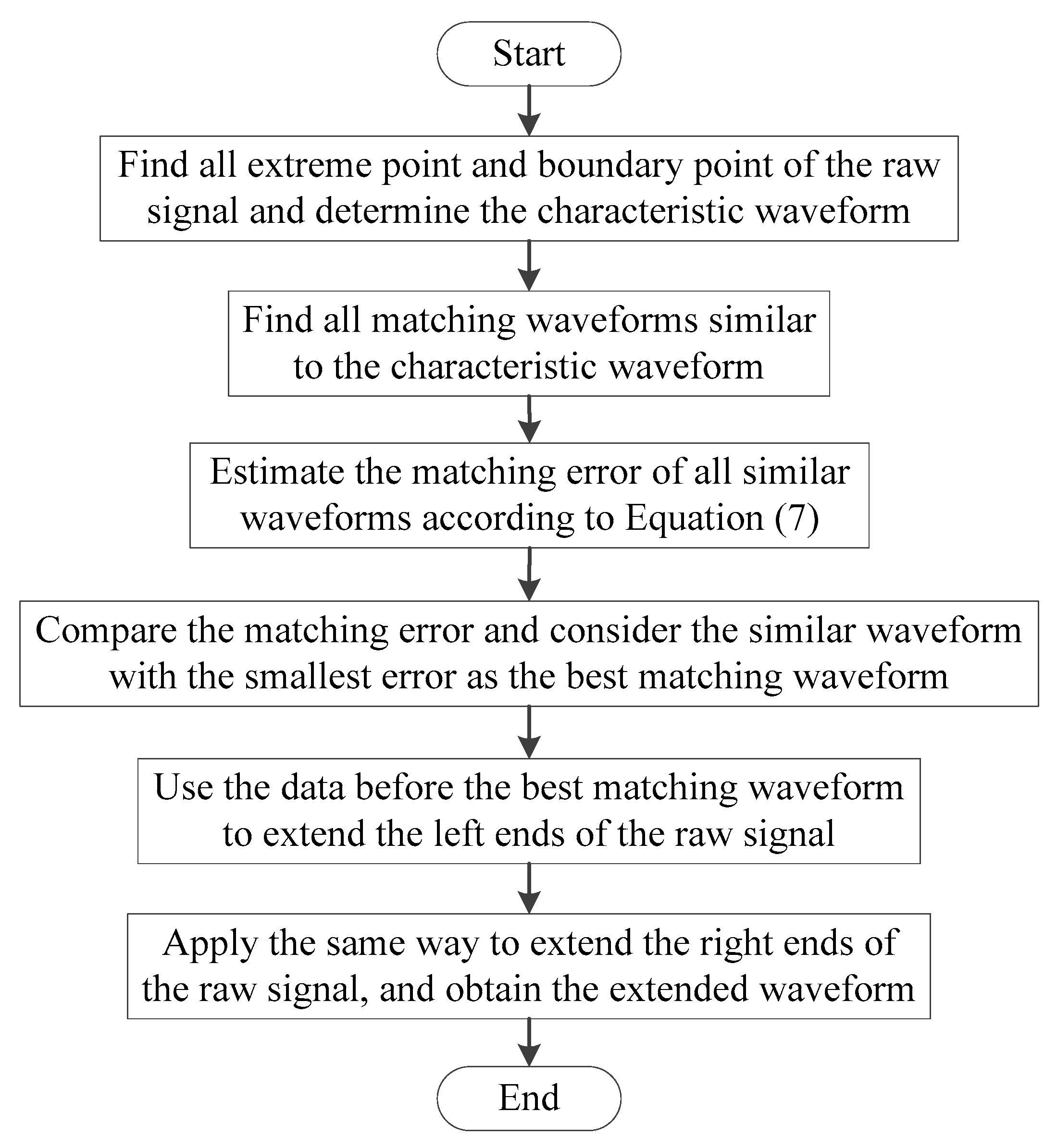
In the waveform matching extension, we first look for all available similar waveforms, then pick out the best matching waveform within them. Last, we connect the waveband before/after the best matching waveform to both left and right ends of the raw waveform to finish the task of boundary processing. Figure 1 shows the flowchart of the waveform matching extension. For one compound waveform x(t), the waveform matching extension procedure is described below [56].

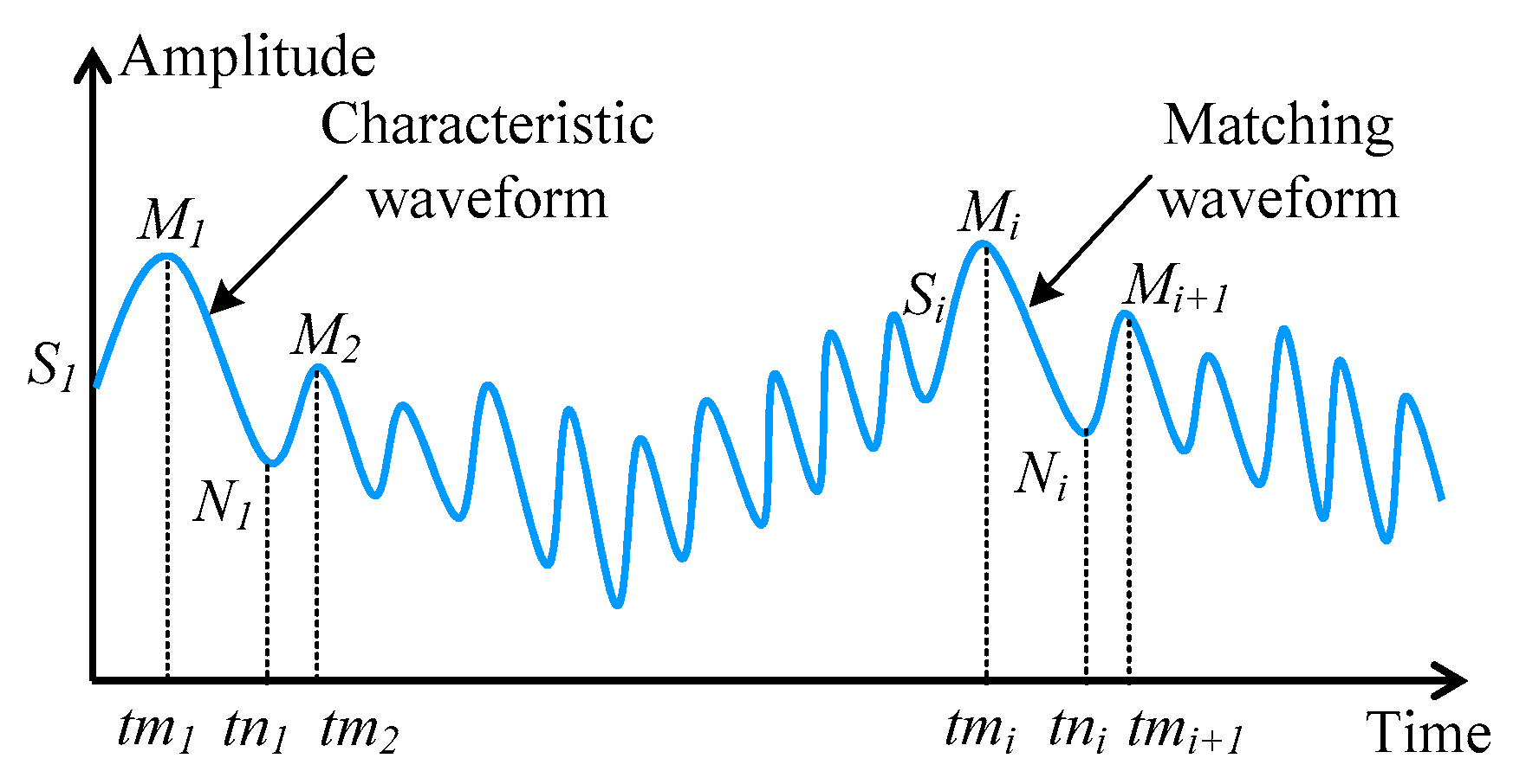
(1) Find all extreme points and boundary points of the original signal x(t) through the peak searching method, and determine the characteristic waveform. Take Figure 2 for an example, $M_i(i=1,2,3,\cdots )$ is the maximum value of x(t), corresponding to the time $t{m}_i$, $N_i$ is the minimum value of x(t), corresponding to the time $t{n}_i$, and $S_1$ is the left boundary point of the signal x(t). We regard the triangular waveform $S_1-M_1-N_1$ of the original signal x(t) as the characteristic waveform to search the optimum matching waveform.

(2) Seek for all matching waveforms resembling the characteristic waveform $S_1-M_1-N_1$ on the basis of the time $t{s}_i$ corresponding to the starting value $S_i$ of the matching waveforms, where the time $t{s}_i$ of the horizontal axis is achieved by the linear interpolation, which is expressed as:

$$t{s}_i=\frac{t{m}_1\times t{n}_i-t{n}_1\times t{m}_i}{t{m}_1-t{n}_1}$$

(6)

(3) Estimate the matching error generated in searching all similar waveforms according to the following Equation (7):

$$E_i=\left|S_i-S_1\right|+\left|N_i-N_1\right|+\left|M_i-M_1\right|+\left|M_{i+1}-M_2\right|$$

(7)

where $\left|M_{i+1}-M_2\right|$ represents the trend term of the similar waveforms, which can reveal the relative extremum position of all similar waveforms.

(4) Compare the matching error, determine the smallest error, and consider the similar waveform $S_1-M_1-N_1$ containing the smallest error as the best matching waveform.

(5) Use the data before the best matching waveform to extend the left ends of the raw waveform x(t).

(6) Apply the same way to extend the right ends of the raw waveform x(t), and finally obtain the extended waveform. This indicates that the waveform matching extension procedure of the original signal x(t) is finished in this stage. That is, the left and right boundaries of the original signal x(t) have been processed thoroughly.

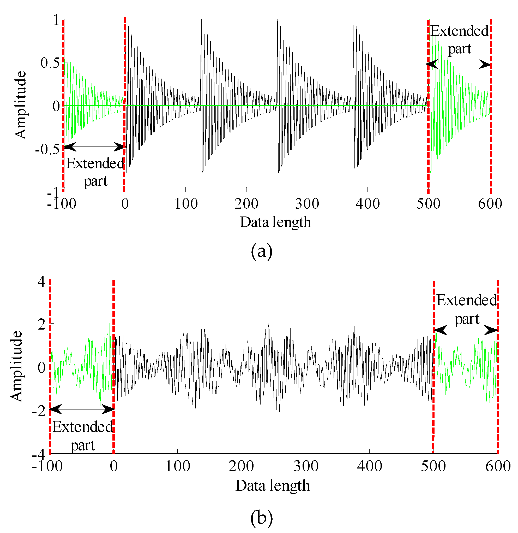
Here, two representative examples for a signal with an abrupt change are utilized to describe intuitively the procedure of waveform matching extension. Without loss of generality, the number of data points extended in both left and right ends are selected as 100 points. Figure 3a,b shows the processing results achieved when applying the waveform matching extension for a cycle shock pulse signal and a modulated compound signal, respectively. Obviously, the waveform extended in both the left and right ends is in line with the variation trend of the raw signal, which indicates that the waveform matching extension is feasible in analyzing the modulated compound signal.

3.2. Parameter Optimization of VMD Using GWO

Two important variables (i.e., the penalty factor $\widehat{\alpha }$ and mode number K) are required to define in advance when we employ VMD to a process complex compound signal. Some previous studies have shown that the two variables ($\widehat{\alpha }$ and K) have a great influence on the decomposition performance of VMD. On the one hand, the bigger $\widehat{\alpha }$ represents the smaller bandwidth of modes. Otherwise, the smaller $\widehat{\alpha }$ represents the greater bandwidth of modes. On the other hand, if the mode number K is too big, it easily leads to the over decomposition phenomenon (i.e., information redundancy), while this will cause the under-decomposition phenomenon (i.e., information loss) when the mode number K is too small. Hence, how to pick out the appropriate variables ($\widehat{\alpha }$, K), is a challenge when applying VMD to deal with complex compound signals. To address this issue, a new nature-inspired algorithm called GWO is introduced to determine and select automatically the combination parameters ($\widehat{\alpha }$, K) of VMD in this subsection due to its excellent global optimization performance. Obviously, the objective function should be constructed when we use GWO to optimize the parameters of VMD. At present, there are many indicators (e.g., smoothness index, entropy, sparseness, kurtosis, and correlation coefficient) in the analysis of the mechanical vibration signal, but it is not optimal to use any of their single indicators to measure vibration signal characteristics. This indicates that the combination of two or more of their single indicators is valuable for practical vibration detection. Zhang et al. [57] presented a new combination index named weighted kurtosis (WK) as the objective function of their method to optimize the key parameters of VMD, but the proposed weighted kurtosis does not consider some abnormal impacts (i.e., the outlier) with disperse distributions. Hence, to solve this problem, a comprehensive evaluation indicator named weighted sparseness kurtosis (WSK) is formulated in this paper to work as the objective function of the parameter optimization process of VMD, which is defined by:

$$WSK=S\cdot Kur\cdot \left|\rho \right|$$

(8)

$$S=\frac{\sqrt{\frac{1}{N}{\displaystyle {\sum }_{n=1}^{N}x{(n)}^2}}}{\frac{1}{N}{\displaystyle {\sum }_{n=1}^N\left|x(n)\right|}}$$

(9)

$$Kur=\frac{\frac{1}{N}{\displaystyle {\sum }_{n=0}^{N-1}{x}^4(n)}}{{\left(\frac{1}{N}{\displaystyle {\sum }_{n=1}^{N-1}{x}^2(n)}\right)}^2}$$

(10)

$$\rho =\frac{E[(x-\overline{x})(y-\overline{y})]}{E[{(x-\overline{x})}^2]E[{(y-\overline{y})}^2]}$$

(11)

where S is the sparseness of the signal x(n), N is the length of the signal x(n), $\rho$ represents the Pearson correlation coefficient between two signals (i.e., x and y) and satisfies $\left|\rho \right|\le 1$, and $E[\cdot ]$ denotes the expectation operator. This indicates that the correlation coefficient $\rho$ amounts to the weight of the sparseness kurtosis indicator. That is, Equation (8) is reputed essentially as the weighted sparseness kurtosis indicator in this paper. Note that in Equation (8) the sparseness is a statistical indicator reflecting the amplitude distribution of the signal, especially for an abnormal impact amplitude with discrete distribution, while kurtosis is very sensitive to the periodic impulse series of vibration signals. Besides, the correlation coefficient can measure the similarity between two vibration signals.

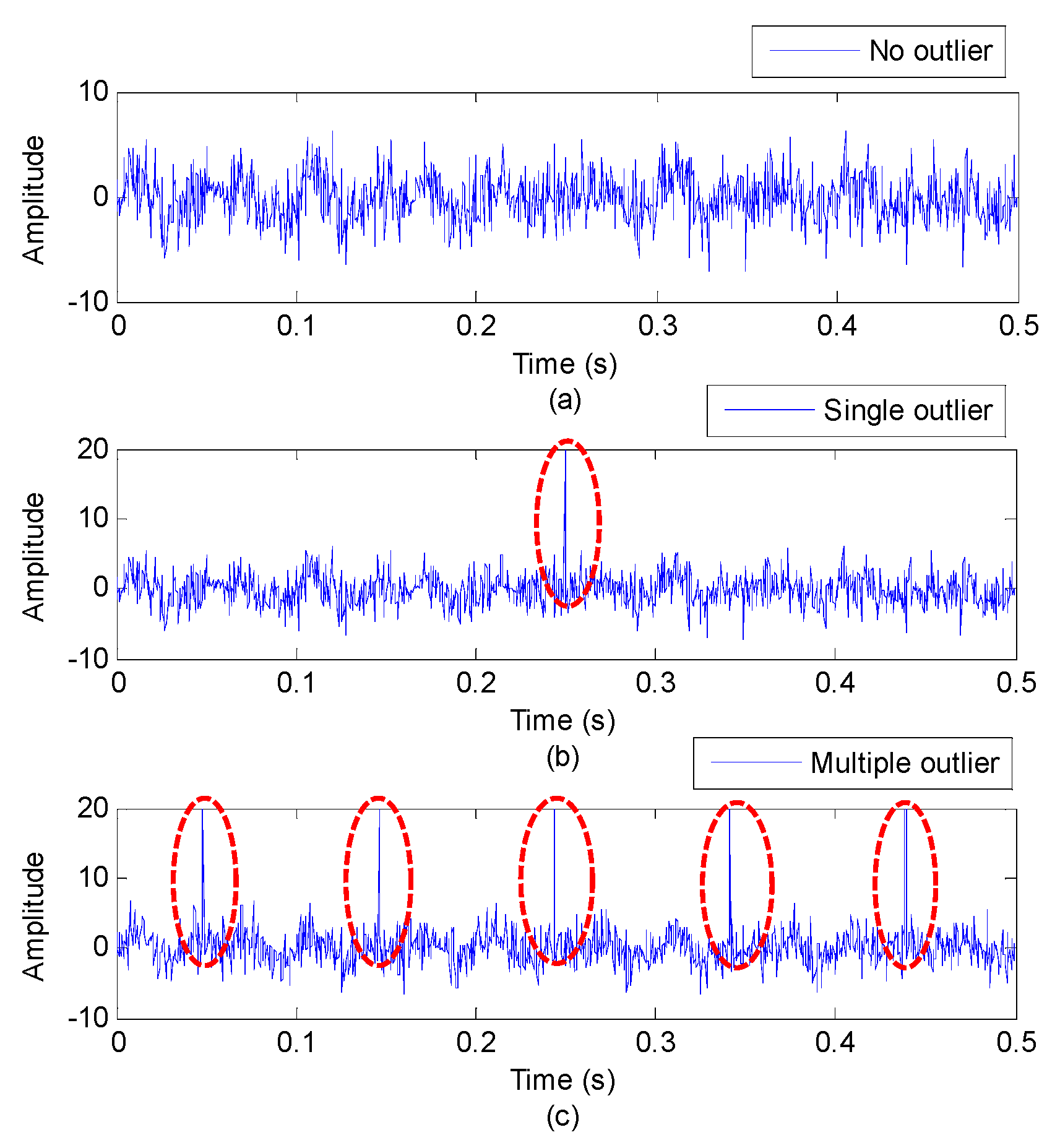
To prove the efficacy of the presented WSK indicator, comparisons between four indicators (i.e., kurtosis, entropy, WK, and WSK) are conducted by analyzing a simulation signal. The simulation signal shown in Figure 4a is composed of the periodic impulse, harmonic signal, and random noise. Figure 4b,c shows the simulation signal containing a single outlier and multiple outlier, respectively.

Table 1. The comparisons among different indicators.

Signal	Kurtosis	Entropy	WK	WSK
No outlier	3.19	6.89	3.19	9.18
Single outlier	7.82	6.58	6.35	9.35
Multiple outlier	16.41	6.32	2.87	9.29

gives the comparison results of different indicators for the simulation signal. From the chart we know that the proposed WSK indicator has the smallest change when the outlier of the signal increases gradually. This implies that the proposed WSK indicator is more reliable and robust to the outlier of the signal compared with the single indicator and WK. Hence, through the combination of three indicators (i.e., the sparseness, kurtosis, and correlation coefficient), the WSK indicator is more comprehensive and has more advantages in measuring vibration features.

Obviously, a larger WSK implies a richer impact feature and a better signal sparseness and decomposition results. Here, to further ensure a global optimal solution, we deem the mean of the WSK of modes acquired by VMD as an objective function of the optimization procedure. Concretely, the goal of the parameter optimization process of VMD using GWO is visually interpreted as an effective search for the minimum value of the opposite of the objective function, as shown in Equation (12):

$$\{\begin{array}{c}fitness=\underset{\gamma =(K,\widehat{\alpha })}{\min }\{-mean(WS{K}_i)\}\\ s.t.K=2,3,\cdots ,8and\widehat{\alpha }=[100,2000]\end{array}$$

(12)

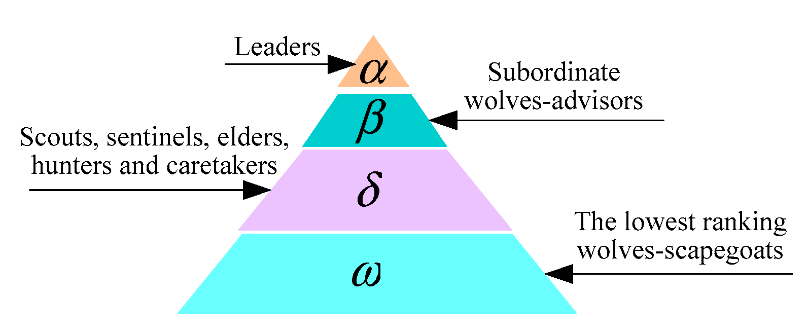
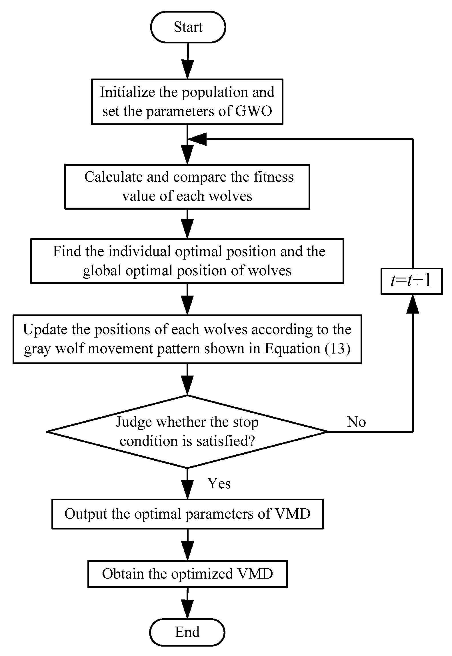
where K denotes the mode number, $\widehat{\alpha }$ denotes the penalty factor, $mean(WS{K}_i)$ is the mean value of WSK, and $WS{K}_i$ is the WSK corresponding to the i-th mode. GWO has a strict population hierarchy, which is mainly divided into four layers (see Figure 5), where the first layer is $\alpha$ (i.e., leaders/the optimal solution), the second layer is $\beta$ (i.e., subordinate wolves-advisors/the suboptimal solution), the third layer is $\delta$ (i.e., scouts, sentinels, elders, hunters, and caretakers/the third optimal solution), and the last layer is $\omega$ (i.e., lowest ranking wolves-scapegoats/other solutions). Moreover, GWO is applied for parameter optimization by implementing several steps (e.g., hunting, searching for prey, encircling prey, and attacking prey). Figure 6 shows the flowchart of the parameter optimization of VMD using the GWO method. The general procedure of VMD parameter optimization is elaborated in detail below:

(1) Initialize the grey wolf population $X_i(i=1,2,\cdots ,m)$, and set the fitness function and the parameters of the GWO algorithm. Generally speaking, the higher the number of wolves and iterations is, the better the optimization results are, but the longer the computation time is; thus, according to Ref. [42], we define the maximum number of wolves m = 30 and maximum iterations T = 10, which is aimed at achieving a tradeoff between the optimization results and computational efficiency. Besides, due to the pre-optimization, the objective only involves two variables ($\widehat{\alpha }$, K), and thus each wolf is expressed as $X_i=(x_K,x_{alpha})$, $i=1,2,\cdots ,m$, where $x_K$ and $x_{alpha}$ represent the penalty factor and mode number, respectively. Due to fault feature information of the practical signal usually spread over the first few high-frequency components obtained by VMD, the first two to eight components are usually selected and analyzed. Besides, the feature information of the main components obtained by VMD is distributed over an appropriate bandwidth, which means that the parameter $\widehat{\alpha }$ is supposed to stay within an empirical range and is neither too big nor too small compared to the default of VMD. For all those reasons, here the search ranges of the two parameters $\widehat{\alpha }$ and K are empirically set as [2, 8] and [100, 2000], respectively.

(2) Calculate the fitness value $mean(WS{K}_i)$ of each wolf $X_i(i=1,2,\cdots ,m)$, look for the minimum fitness value (i.e., $\min \{mean(WS{K}_i)\}$) between the four agents (i.e., the fitness value of the individual grey wolf $\alpha$, $\beta$, $\delta$, and $\omega$) and record the current best wolves $X_{best}$.

(3) Update the position of wolves in terms of the gray wolf movement pattern shown in Equation (13):

$$X_i(t+1)=\frac{X_{i,\alpha }(t)+X_{i,\beta }(t)+X_{i,\delta }(t)}{3}$$

(13)

$$\{\begin{array}{c}{X}_{i,\alpha }(t+1)=X_{\alpha }(t)-A\cdot \left|C\cdot X_{\alpha }(t)-X_i(t)\right|\\ X_{i,\beta }(t+1)=X_{\beta }(t)-A\cdot \left|C\cdot X_{\beta }(t)-X_i(t)\right|\\ X_{i,\delta }(t+1)=X_{\delta }(t)-A\cdot \left|C\cdot X_{\delta }(t)-X_i(t)\right|\end{array}$$

(14)

where A is the convergence factor and meets $A=2d\cdot r_1-d$, C is the swing factor and meets $C=2\cdot r_2$, d is the range control parameter which linearly decays from 2 to 0 over the whole iteration, and $r_1$ and $r_2$ are the random numbers between 0 and 1.

(4) Calculate the fitness value $mean(WS{K}_i{}^{\mathrm{new}})$ of new wolves, and record the best wolves $X_{best}^{new}$ through the comparison of the fitness value. That is, if the fitness value $mean(WS{K}_i)$ of the updated wolves overmatches that of the previous wolves, the updated wolves $X_i^{(t+1)}$ will take the place of the previous wolves $X_i^{(t)}$. Otherwise, retain the previous wolves $X_i^{(t)}$.

(5) Determine whether the stopping condition is satisfied. Concretely, decide whether the current iterations are lower than the maximum iterations (i.e., $t\le T$) or whether the opposite of the fitness value $mean(WS{K}_i)$ is small enough. If that is the case, stop the iteration and output the best wolves $X_{best}$ (i.e., the best parameters $x_{alpha}^{best}$ and $x_K^{best}$ of VMD). Otherwise, let t = t + 1, back to step (2) to keep working.

In short, this section has two contributions. First, the WSK indicator is proposed and is more reliable and robust to the outlier of the signal compared with the previous WK and three single indicators (i.e., the sparseness, kurtosis, and correlation coefficient). Second, two key parameters ($\widehat{\alpha }$, K) of VMD can be determined automatically by using the GWO method, where the mean of the proposed WSK for all modes is regarded as the objective function of the optimization procedure.

3.3. Teager Energy Operator

For a given continuous-time signal with modulated information $x(t)=a(t)\cos (\varphi (t))$, TEO is defined as:

$$\psi [x(t)]={[\dot{x}(t)]}^2-x(t)\ddot{x}(t)$$

(15)

where $\dot{x}(t)$ and $\ddot{x}(t)$ mean the first and second order derivative functions of x(t), respectively. For a discrete signal x(n), TEO is modified into $\psi [x(n)]=x^2(n)-x(n-1)x(n+1)$, where n means the length of x(n). The instantaneous amplitudes IA and IF of x(n) are capable of being acquired using the discrete energy separation method (see the DESA-2 function in MATLAB), as shown in Equations (16) and (17):

$$a(n)=\frac{2\psi [x(n)]}{\sqrt{\psi [x(n+1)-x(n-1)]}}$$

(16)

$$f(n)=\frac{1}{4\pi }\arccos \left(1-\frac{\psi [x(n+1)-x(n-1)]}{2\psi [x(n)]}\right)$$

(17)

where $a(n)$ represents the instantaneous amplitude, and f(n) represents the instantaneous frequency. One major advantage of TEO compared with HT is that the calculated IA and IF have fewer errors.

3.4. The Proposed IAVMD Method

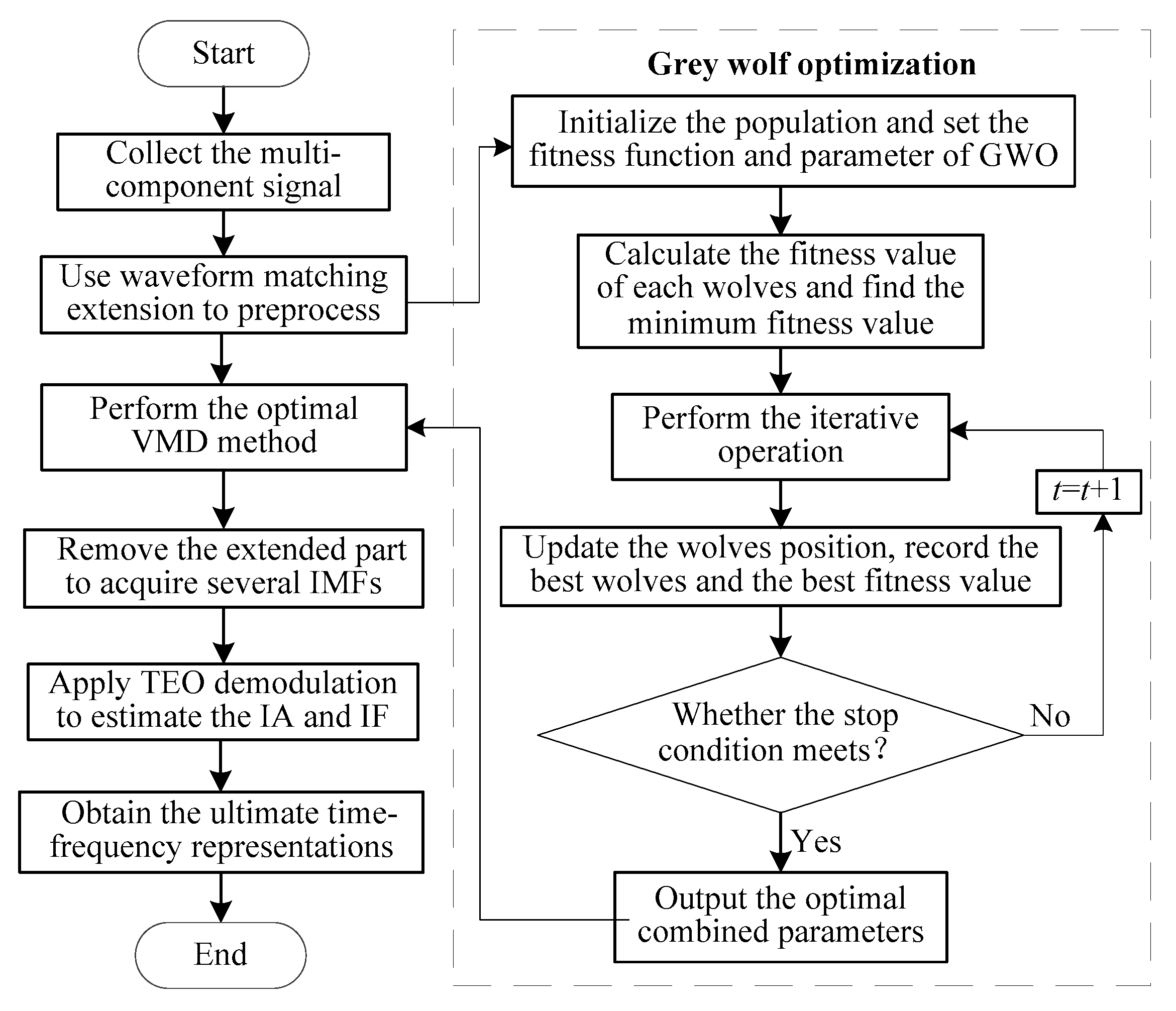
As mentioned before, the advantages of waveform matching extension are utilized by this paper for signal pretreatment. The inside parameters (i.e., $\widehat{\alpha }$ and K) of VMD are determined beforehand by GWO, which can make the algorithm adaptive and practicable. One advantage of TEO is that the edge errors of HT can be avoided in the signal demodulation process. Hence, by merging together several procedures, a novel TFA method called IAVMD is formulated in this paper. Figure 7 shows the flowchart of the proposed method. For a multi-component signal, the realization process of the proposed IAVMD method is as follows:

Step 1: Preparations of IAVMD. Use the waveform matching extension illustrated in Figure 1 to stretch the left and right boundary points of the multi-component signal.

Step 2: Parameter optimization automatically. Introduce GWO to adaptively search the optimal inside parameters ($\widehat{\alpha }$, K) of VMD according to steps (1) to (5) of Section 3.2.

Step 3: Signal decomposition. Apply the parameter optimization VMD method to decompose the extended signal acquired by step 1 into several IMF components shown in Equation (3), and truncate the extended data points of each IMF component to obtain the final decomposition results.

Step 4: Signal demodulation. Perform TEO to estimate the IF and IA of each IMF component, and plot the IF of all IMF components together to get the ultimate time-frequency representations of the original signal. Observe and identify the frequency contents displayed in TFR, and output the fault diagnosis results.

4. Simulation Validation

4.1. Case 1: Sinusoidal Superposition Signal

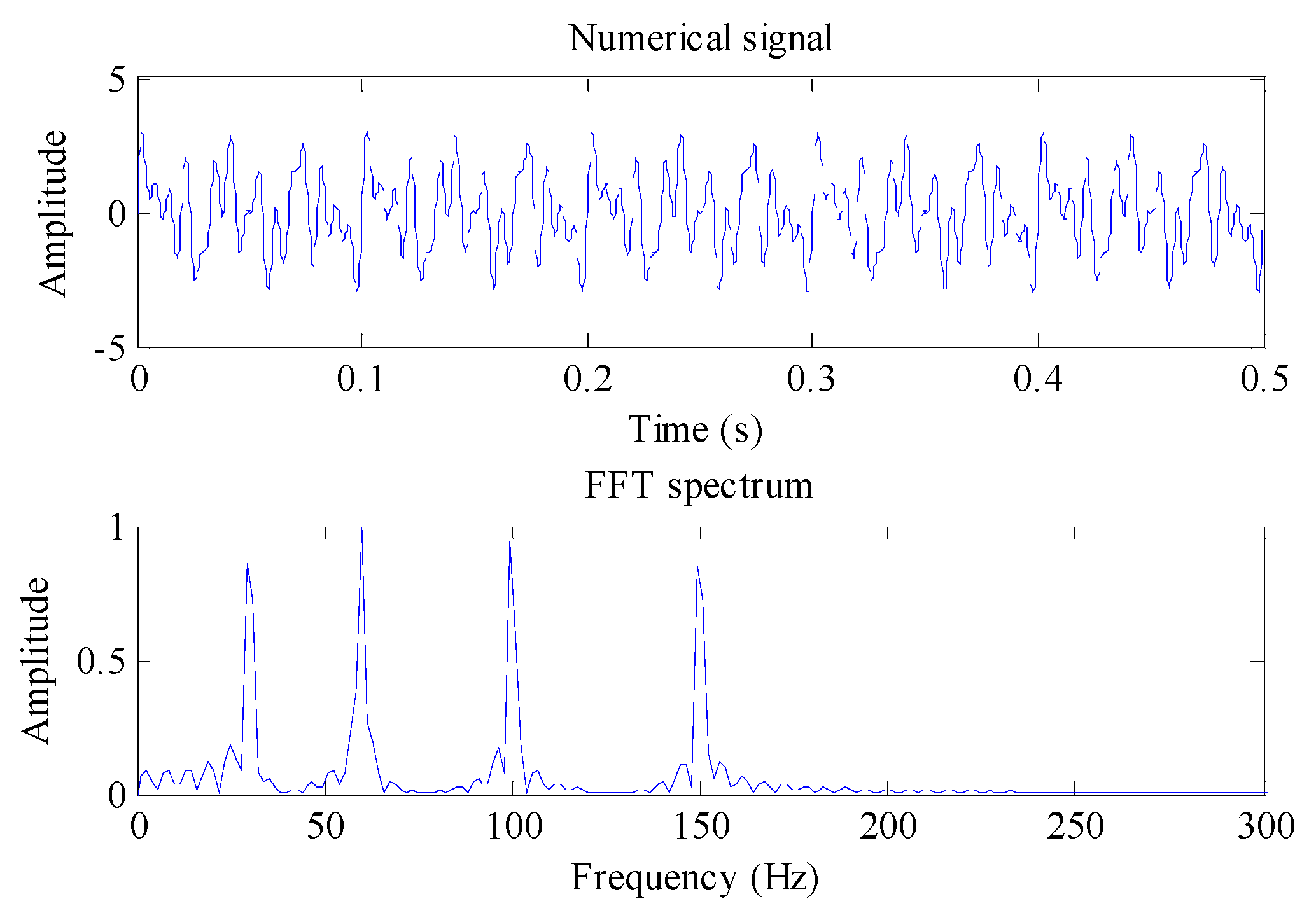
Considering that the real rotor vibration signal is generally expressed as multiple harmonic superposition signals (e.g., the linear superposition of fundamental frequency, fractional frequency, and ultraharmonics), to confirm the availability of the presented approach we here employ a numerical signal $y(t)$ consisting of four sine waves (their frequencies are, respectively, 30 Hz, 60 Hz, 100 Hz, and 150 Hz) to simulate the rotor fault signal, which is considered as follows:

$$\begin{array}{l}y(t)=x_1(t)+x_2(t)+x_3(t)+x_4(t)\\ \hspace{1em}\hspace{1em}=\sin (60\pi t)+\sin (120\pi t)+\sin (200\pi t)+\sin (300\pi t)\end{array}$$

(18)

where $x_1(t)$ is used to simulate the fundamental frequency component of the rotor fault signal, $x_2(t)$ is used to simulate the double frequency component of the rotor fault signal, $x_3(t)$ is used to simulate the fractional frequency component of the rotor fault signal, and $x_4(t)$ is used to simulate the higher harmonic component of the rotor fault signal. For the simulation signal $y(t)$, its sampling frequency and sampling number are set as 3000 Hz and 1500, respectively. Figure 8 draws the numerical signal $x(t)$ and its FFT spectrum.

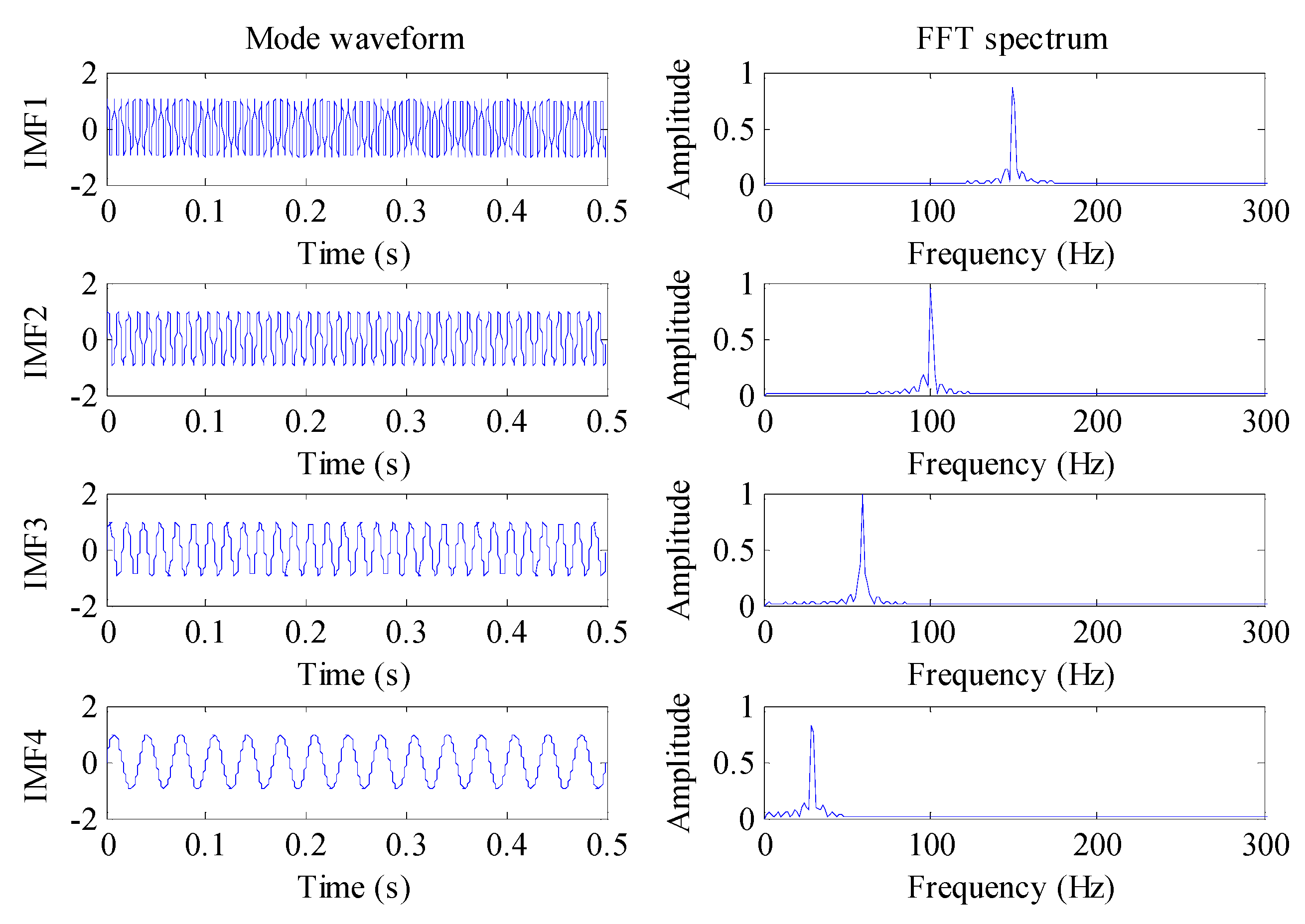
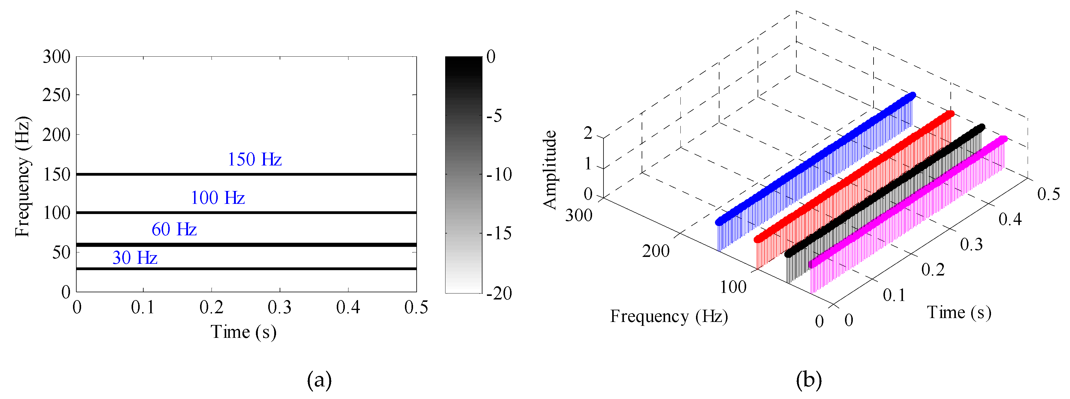
In the IAVMD method, the numerical signal $y(t)$ is first preprocessed by waveform matching extension, after which the optimal combined parameters ($\widehat{\alpha }$, K) of VMD obtained using GWO are (1986, 4). That is, VMD with $\widehat{\alpha }$ = 1986 and K = 4 is applied to analyze the numerical signal $y(t)$, and the ultimate decomposition results are shown in Figure 9. Note that, except for the input signal and two key parameters ($\widehat{\alpha }$, K), another four parameters (e.g., time-step of the dual ascent $\tau$, DC part, uniform initialization of omegas, and tolerance of the convergence criterion $\epsilon$) of VMD have a fixed value, set as 0, 0, 0, and 10⁻⁶, respectively. Seen from Figure 9, four frequency components of the numerical signal $y(t)$ are separated efficiently. Figure 10a,b plots the two-dimensional and three-dimensional TFR based on IAVMD, respectively. One can clearly see that the time-frequency trajectory obtained by IAVMD is very clear in Figure 10, which indicates that the proposed IAVMD can exactly decompose the sinusoidal superposition signal containing multiple components.

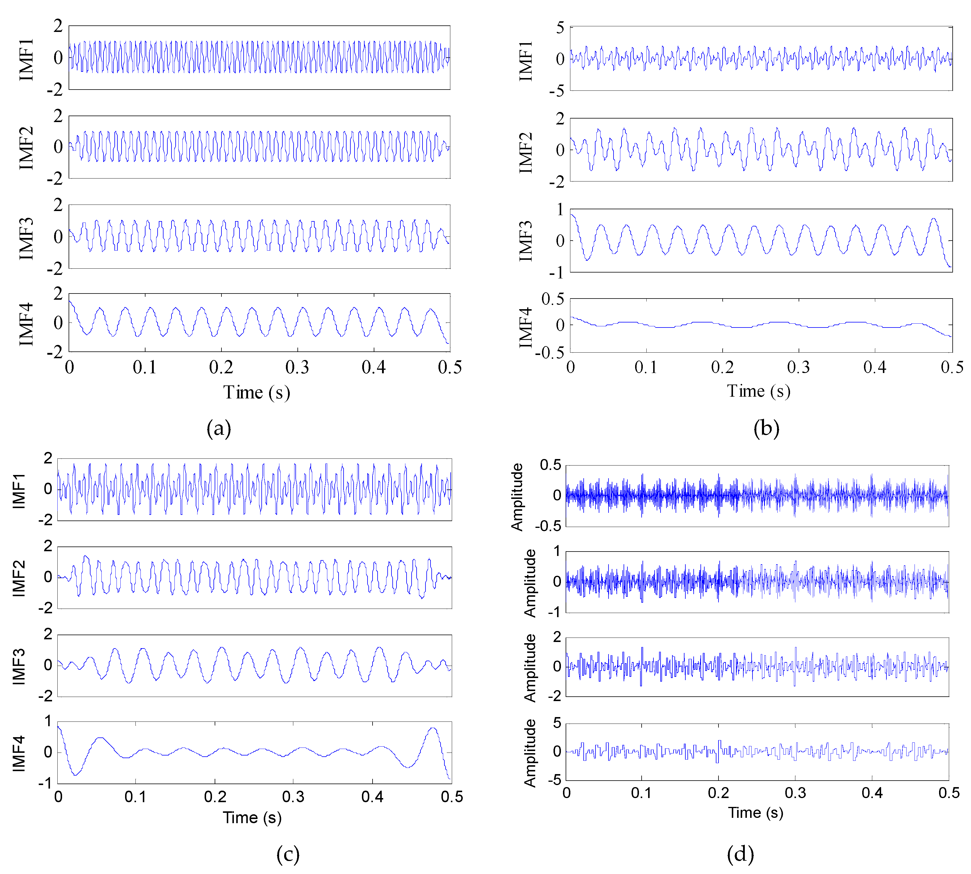
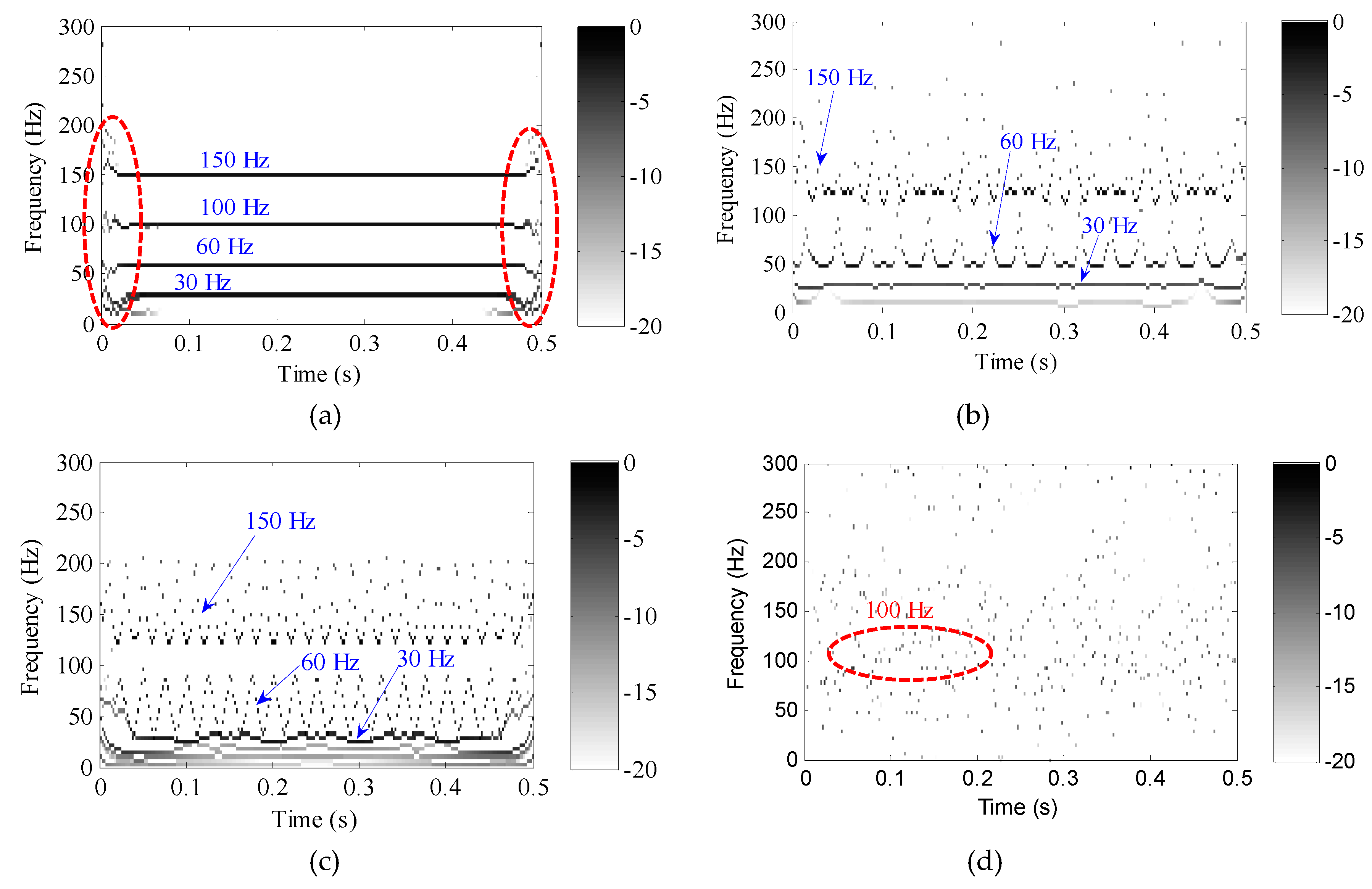
As a comparison, particle swarm optimization-based VMD (OVMD) and three other techniques (i.e., LMD, EMD, and WT) are devoted to disposing the same signal $y(t)$. The optimization range of OVMD is the same as for the proposed method. Here, the optimized parameters of OVMD are respectively determined as $\widehat{\alpha }$ = 1120 and K = 4 by using the PSO algorithm. The decomposition results acquired by OVMD, LMD, EMD, and WT are shown in Figure 11a–d, respectively. Besides, the acquired TFR using four techniques (i.e., OVMD, LMD, EMD, and WT) are shown in Figure 12a–d, respectively. Note that, in the comparison process, to ensure a fair comparison, the TFR of four methods (i.e., OVMD, LMD, EMD, and WT) are obtained by TEO, where WT adopts the ‘db1’ wavelet function containing a good orthogonality and where three decomposition layers are performed (i.e., four reconstructed wavelet coefficients can be obtained for implementing the time-frequency analysis). As shown in Figure 12a, four sub-components are extracted effectively, but they suffer from certain boundary fluctuations (see the red dotted line). From Figure 12b,c, one can observe that the first two IMFs suffer from serious mode aliasing and that the signal representation in the time-frequency plane is highly dispersed. That is, the IMFs derived from LMD and EMD cannot coincide well with the real components. As can be seen from Figure 12d, many discrete points appear on the time-frequency trajectory. That is, the time-frequency trajectory obtained by WT is very scattered and unfocused, so it is difficult to effectively identify the frequency components. This means that the time-frequency resolution of WT is not as good as those provided in Figure 10a. Consequently, through the comparison of Figure 12a–d, it is obvious that the potential of our presented IAVMD approach in analyzing non-stationary compound signals is preliminarily verified. Besides, the decomposition performance of our presented IAVMD is superior to that of some classical algorithms mentioned in this case.

4.2. Case 2: AM-FM Superposition Signal

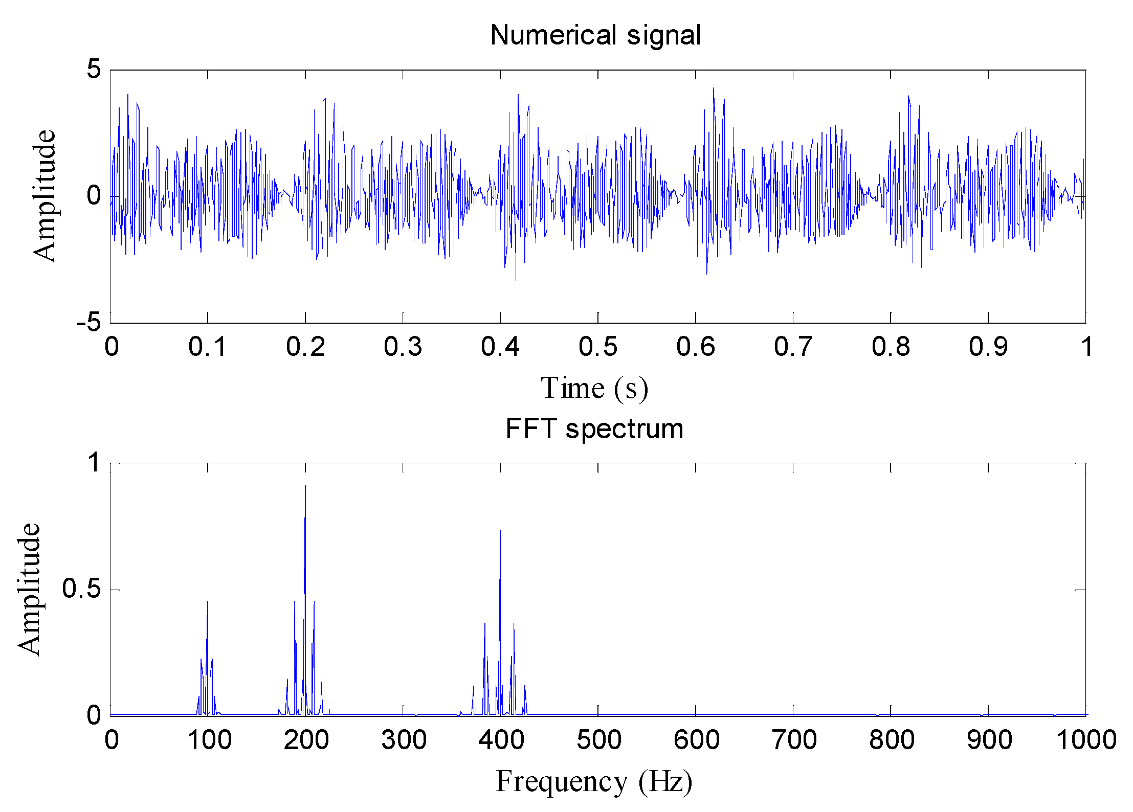
To further prove the efficacy of the proposed IAVMD method, we analyze and investigate a numerical signal $z(t)$ shown in Equation (19), which is composed of three AM-FM signals and a stochastic noise:

$$\{\begin{array}{l}z(t)=q_1(t)+q_2(t)+q_3(t)+q_4(t)\\ q_1(t)=(0.8+0.8\sin (30\pi t))\cos (800\pi t+0.6\sin (24\pi t))\\ q_2(t)=(1+\sin (20\pi t))\cos (400\pi t+0.6\sin (16\pi t))\\ q_3(t)=(0.5+0.5\sin (10\pi t))\cos (200\pi t+0.6\sin (8\pi t))\end{array}$$

(19)

where three components $q_1(t)$, $q_2(t)$, and $q_3(t)$ are AM-FM signals containing the main frequency of 400 Hz, 200 Hz, and 100 Hz, respectively. The component $q_4(t)$ is a stochastic noise added in the numerical signal $z(t)$, and its value is generated by the randn() function in MATLAB. The sampling frequency and sampling number of the simulation signal $z(t)$ are 3000 Hz and 3000, respectively. Figure 13 shows the simulation signal $z(t)$ and its corresponding FFT spectrum.

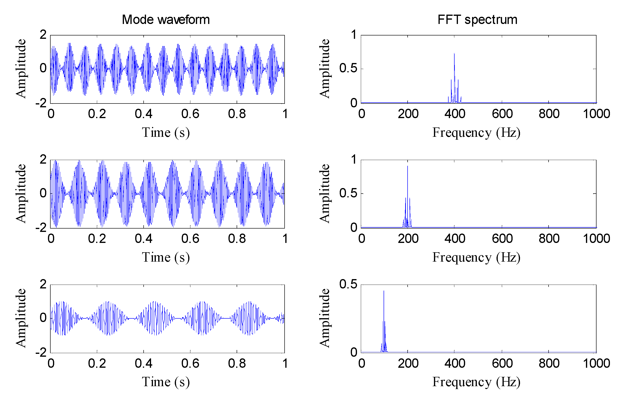
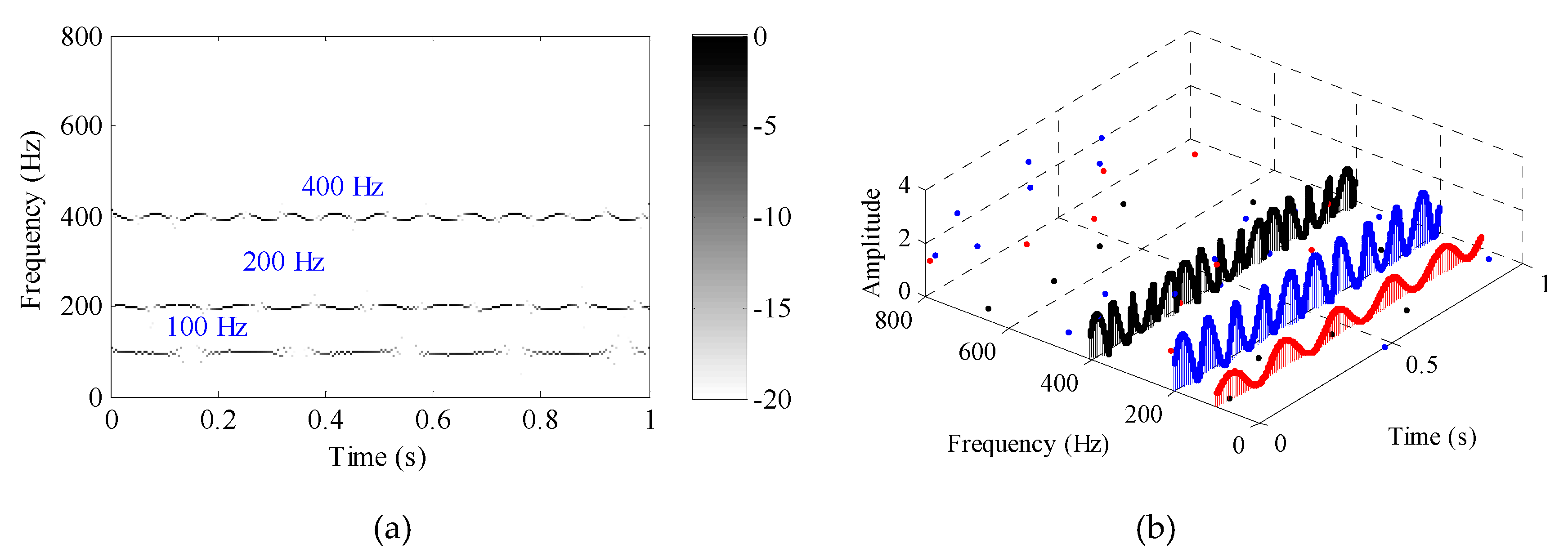
The proposed IAVMD method is adopted to analyze the simulation signal $z(t)$. First, waveform the matching extension is used to preprocess the simulation signal $z(t)$, after which the GWO method is employed to determine automatically the VMD parameters $\widehat{\alpha }$ = 1023 and K = 3. Finally, VMD containing the optimal parameters is adopted to analyze the simulation signal $z(t)$, and the ultimate decomposition results are displayed in Figure 14. The corresponding time-frequency representations are shown in Figure 15. Figure 15a,b shows the two-dimensional and three-dimensional TFR based on IAVMD, respectively. It can be clearly seen from Figure 14 and Figure 15 that three components obtained by the proposed method are very close to three real AM-FM components of the original signal, which indicates that the IAVMD method is effective in analyzing multi-component signals with modulation phenomena.

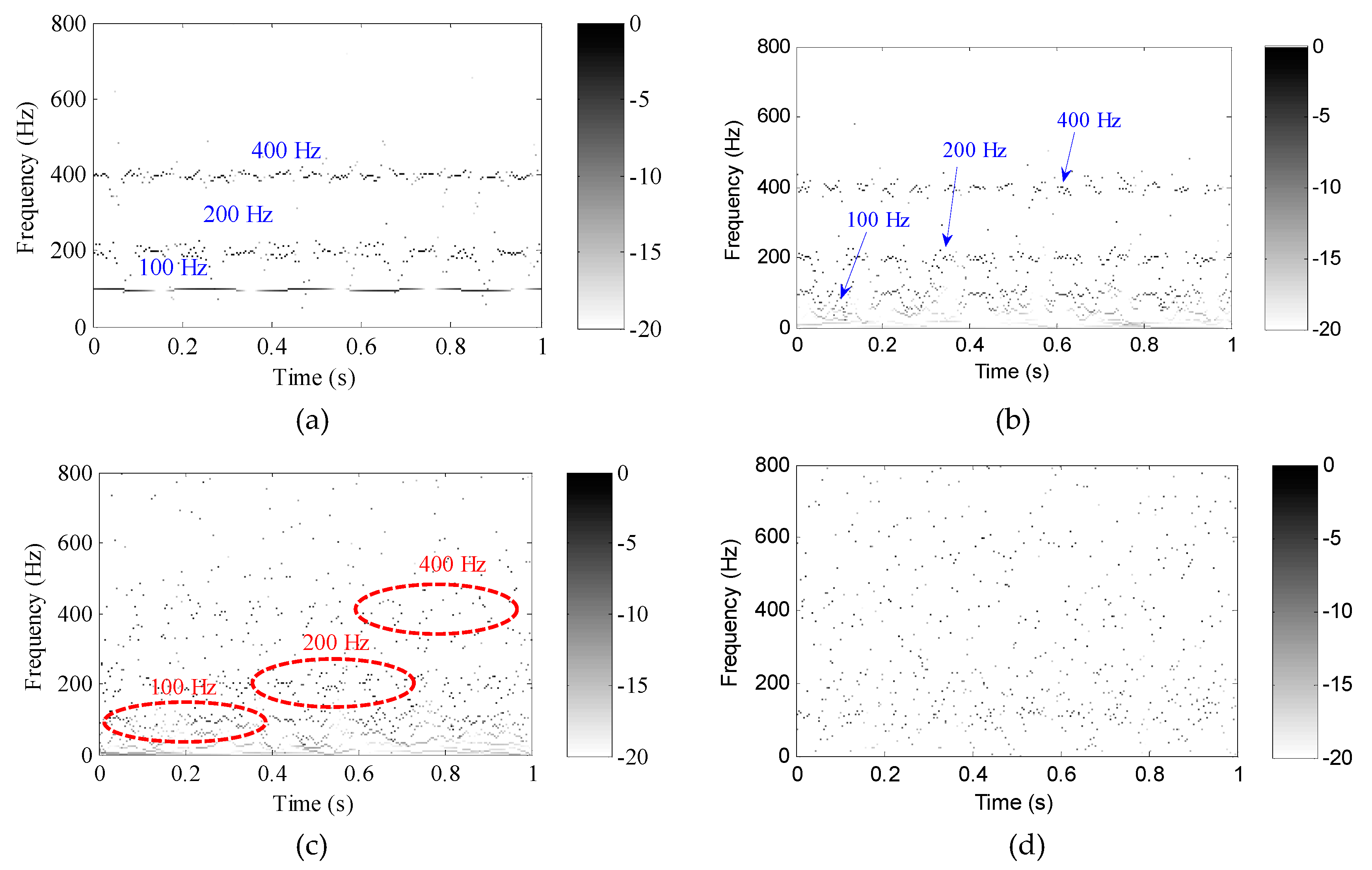
As a contrast, four methods (i.e., OVMD, LMD, EMD, and WT) are employed to deal with the same simulation signal $z(t)$. Note that to consolidate the results of the proposed method two key parameters of OVMD are optimized as $\widehat{\alpha }$ = 751 and K = 3. Besides, the implementation of the TFR of other three methods is the same as that of simulation 1. The TFR obtained by the four methods are plotted in Figure 16a–d, respectively. Seen from Figure 16a, in the first two components obtained by OVMD, there is some deviation from the true component. That is, the first two components have a low resolution in TFR based on OVMD. As shown in Figure 16b,c, the time-frequency trajectory is not clear in the TFR based on EMD and LMD, and their time-frequency aggregation is not as good as in the proposed method. As shown in Figure 16d, the time-frequency trajectories are scattered, and three frequency components of the original signal cannot be identified in TFR based on WT. Therefore, the above comparison results further validate the effectiveness of the proposed method in multi-component signal analysis.

In short, the contribution of this section is that two simulation cases are adopted to verify the effectiveness of our proposed IAVMD method. Besides, the superiority of the IAVMD method is demonstrated via the comparisons of various similar methods (e.g., OVMD, LMD, EMD, and WT).

5. Experimental Validation

5.1. Experiment Platform and Data Description

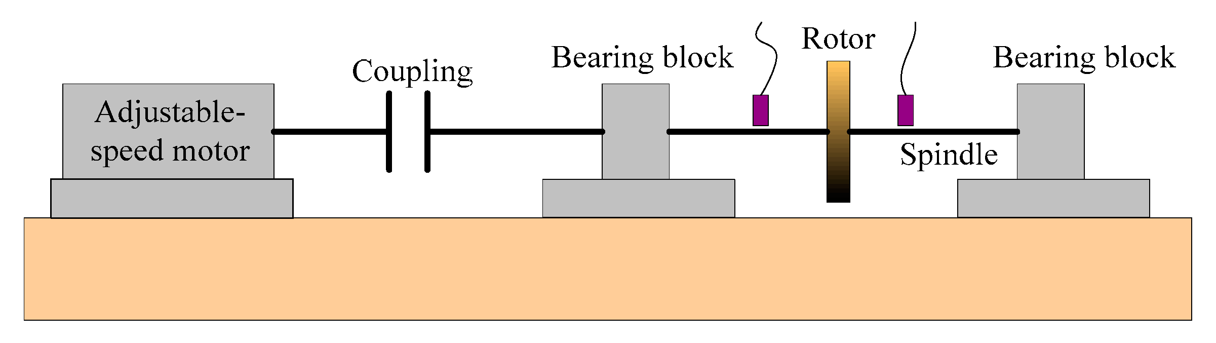
To further verify the presented IAVMD method, we process the experimental data collected from the rotor-bearing system in the vibration measurement laboratory at North China Electric Power University (NCEPU). The experimental device used in the testing is a Bently RK-4 test bench (see Figure 17), which mainly consists of a signal front adapter, speed-adjusting, and a bearing oil pump system. The specification of the data collection equipment is ZonicBook/618E. The eddy current sensor and key phasor transducer are mounted on both sides of the disk to collect the rotor experimental vibration signal and rotational speed signal, respectively. First, plastic rods near the revolving shaft were adopted to produce the slight local rub-impact fault under 1790 r/min (i.e., rotating frequency $f_1$ = 29.83 Hz). Second, the rotor oil-whirl and oil-whip fault were generated by adjusting the device such as the oil pump, preload scaffold, and motor speed controller when the rotation speed was respectively set at 2600 r/min (i.e., rotating frequency $f_2$ = 43.33 Hz) and 4500 r/min (i.e., rotating frequency $f_3$ = 75 Hz). Note that the critical speed of oil-whip is about 1800 r/min (i.e., oil-whip frequency $f_w$ = 30 Hz). Specifically, in this experiment, the rotor system operates at above twice the critical speeds, resulting in rotor oil-whip. The sampling frequency and data length during testing were set at 1280 Hz and 1024 points, respectively. Generally speaking, when the rotor shows a rub-impact fault, the expected main fault feature frequencies in the frequency spectrum are the rotating frequency $f_1$, its harmonics (e.g., 2 $f_1$, 3 $f_1$, and 4 $f_1$) and sub-harmonics (e.g., 0.5 $f_1$, 1.5 $f_1$, and 2.5 $f_1$). Besides, as we know the rotor oil-whirl is also known as half-speed whirl. That is, the expected main fault frequencies in the frequency spectrum are half of the rotating frequency (0.5 $f_2$) and its related harmonics (e.g., $f_2$, 1.5 $f_2$, 2 $f_2$, 2.5 $f_2$, and 3 $f_2$) when the rotor shows oil-whirl. Similarly, the expected main fault frequencies in the frequency spectrum are the oil-whip frequency $f_w$, rotating frequency $f_3$, and their related harmonics (e.g., 0.5, $f_3$ − $f_w$, $f_3$ + $f_w$, 2 $f_w$, + 1.5 $f_w$, and 2 $f_3$) when the rotor shows oil-whip.

5.2. Case 1: Rotor Rub-Impact Fault Detection

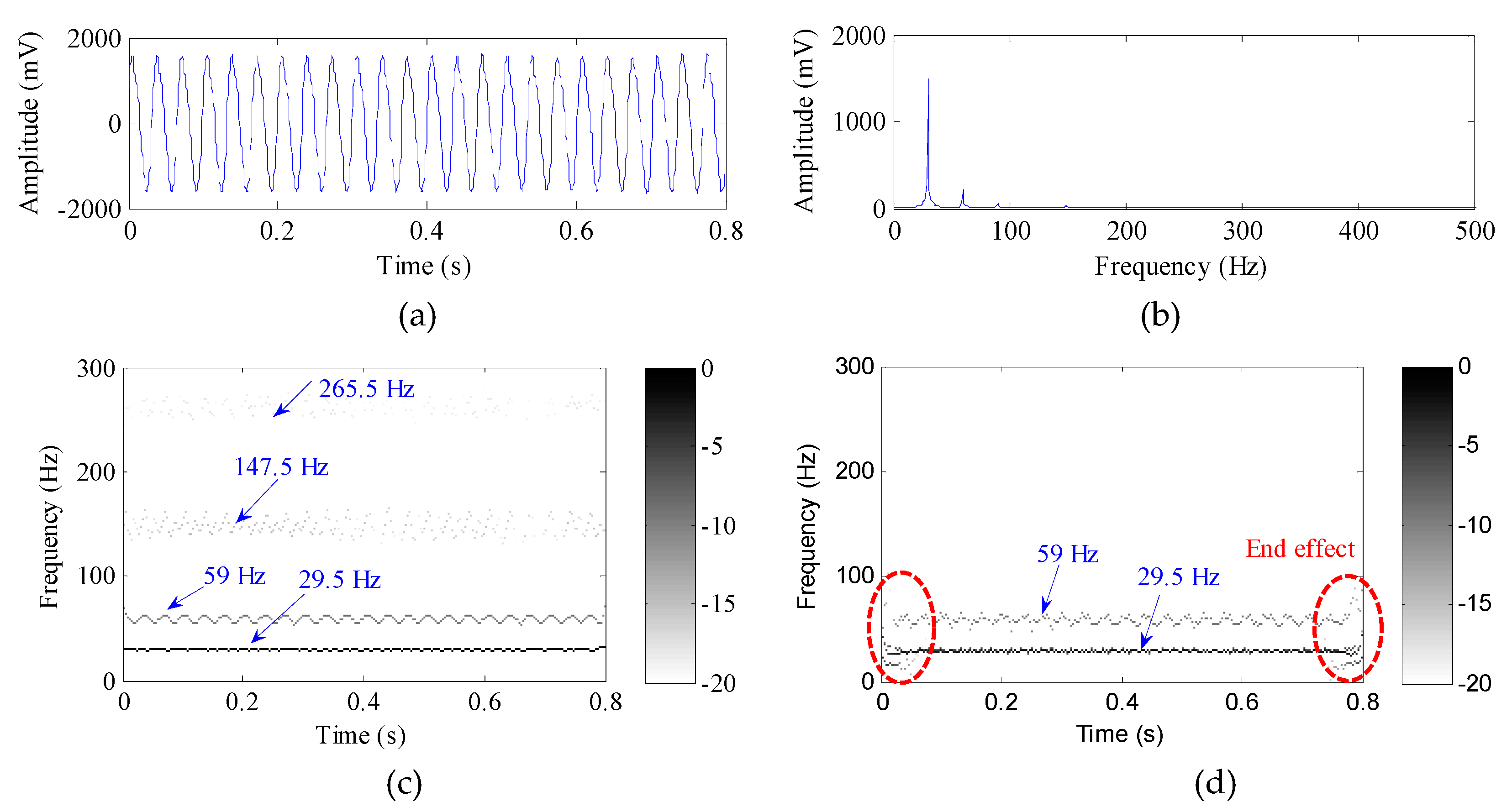
Figure 18a,b shows the waveform and FFT spectrum of the rotor early rub-impact signal, respectively. As seen in Figure 18a,b, the rotor slight rub-impact signal is expressed approximatively by a sine wave, the frequency component of 29.5 Hz (approximately equal to the rotating frequency $f_1$) is very clear in the FFT spectrum, but the amplitude at the harmonics is very small. That is to say, it is not easy to judge whether rub-impact fault occurs when directly using the FFT spectrum.

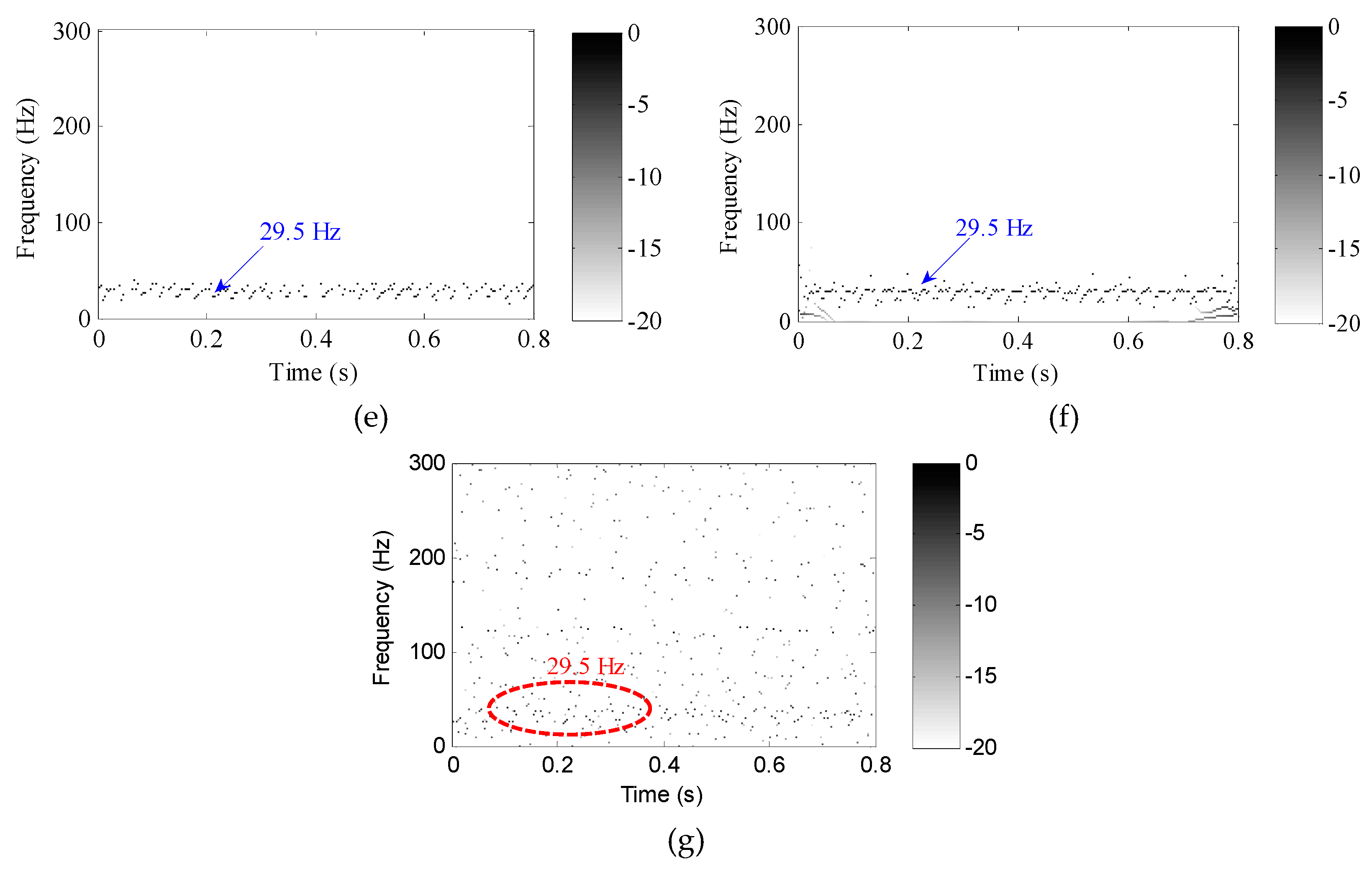
Five approaches (i.e., IAVMD, OVMD, LMD, EMD, and WT) are applied to decompose the rub-impact fault signal, respectively. Figure 18c–g respectively depicts the TFR resulting from the five methods. The optimal inside parameters in IAVMD are selected as $\widehat{\alpha }$ = 1177 and K = 4 through using the GWO algorithm. The optimal parameters of OVMD are determined as $\widehat{\alpha }$ = 536 and K = 4 through using the PSO algorithm. As seen in Figure 18c, the fundamental frequency of 29.5 Hz and its various harmonics (59 Hz, 147.5 Hz, and 265.5 Hz) can be identified. In addition, the high frequency is relatively ambiguous due to a resolution problem, but the spectral line is very clear in the low frequency. This indicates that our presented IAVMD approach can detect early characteristics of rotor rub-impact faults.

As shown in Figure 18d, we can easily find the frequency components of 29.5 Hz and its second-harmonic (59 Hz), but the results have overlap and there is a serious end effect (see the parts marked with a red line). In Figure 18e,f, the instantaneous frequencies of 29.5 Hz can be found, but their time-frequency trajectory is obscure. It is obvious from Figure 18g that the TFR obtained by WT can dimly extract the rotating frequency of 29.5 Hz, but the frequency points are very scattered and their time-frequency resolution is clearly worse. The contrastive analysis demonstrated that the efficacy of IAVMD in rotor rub-impact fault detection is superior to that of the other four approaches (i.e., OVMD, LMD, EMD, and WT).

5.3. Case 2: Rotor Oil-Whirl Fault Detection

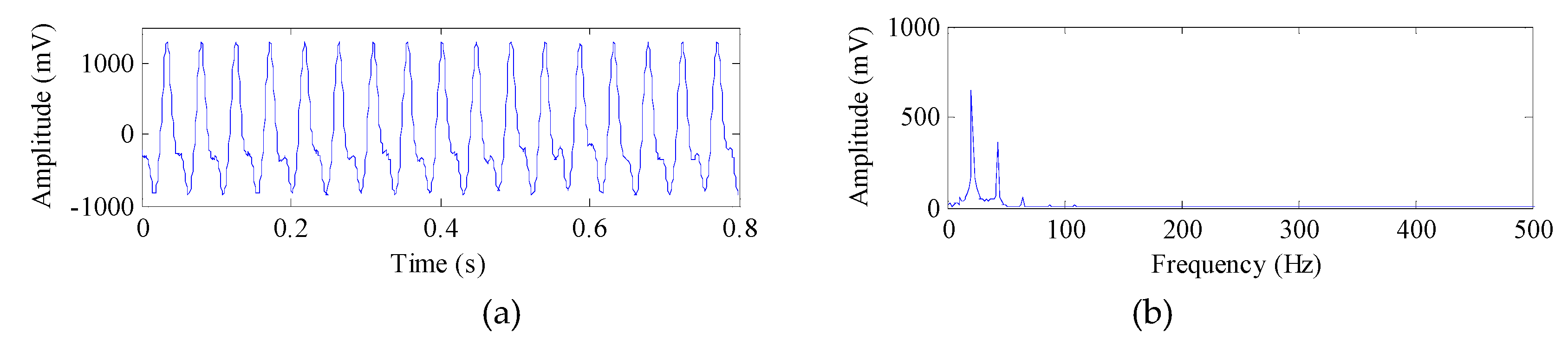
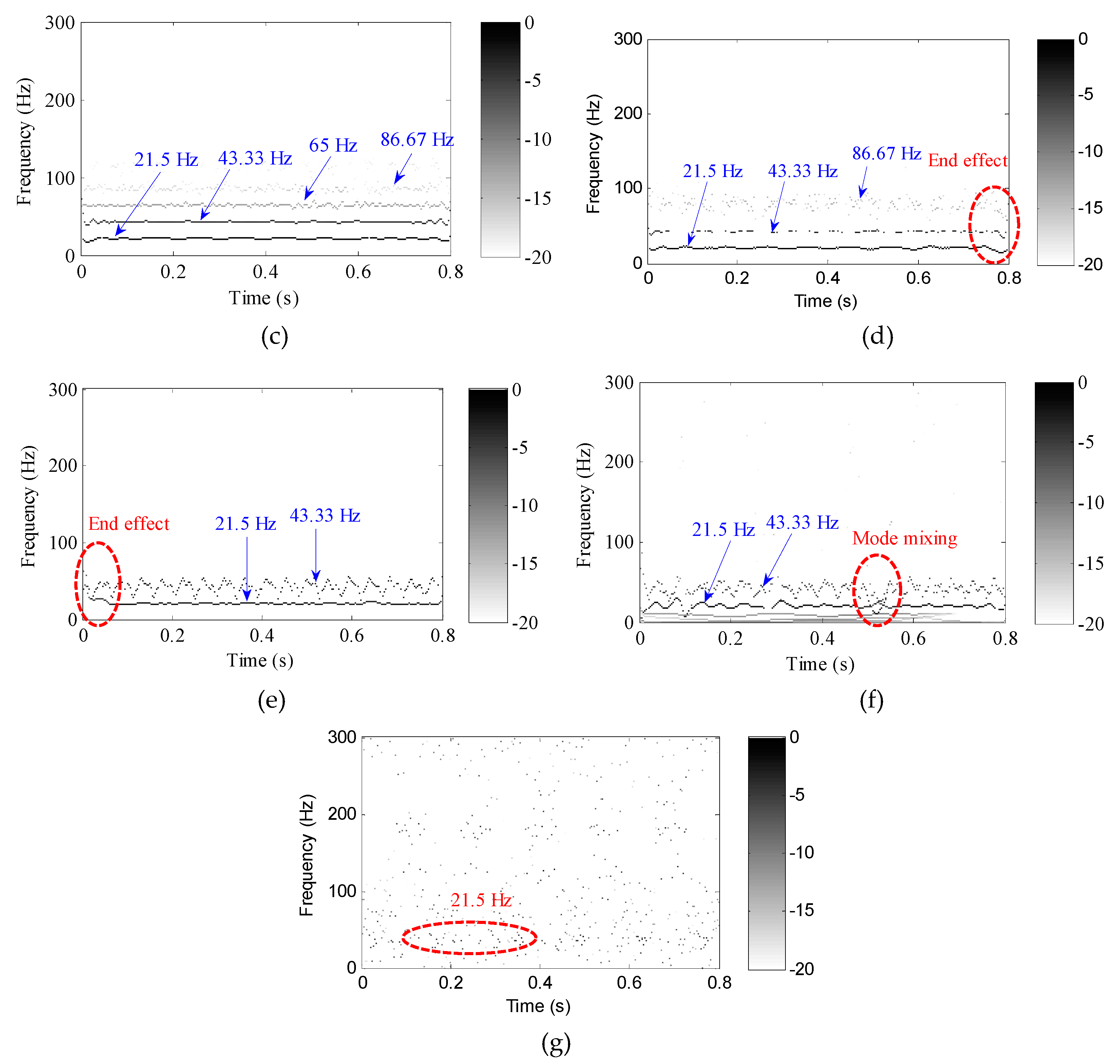
Figure 19a,b shows the waveform and FFT spectrum of the rotor oil-whirl signal, respectively. Figure 19a shows that the rotor oil-whirl signal is represented by a sum of sine waves, and that in the FFT spectrum there is a prominent amplitude at the rotating frequency $f_2$ of 43.33 Hz. Besides, the amplitude of the oil-whirl frequency of 21.5 Hz (equal to about 0.5 $f_2$) is greater than that of the rotating frequency, but the amplitude of the high frequency is not obvious.

The oil-whirl signal is analyzed by five methods (i.e., IAVMD, OVMD, LMD, EMD, and WT), respectively. Figure 19c–g provides the TFR derived from the five methods, respectively. In IAVMD, the optimal parameters obtained by the GWO algorithm are $\widehat{\alpha }$ = 1919 and K = 4, respectively. In OVMD, the optimal parameters are set as $\widehat{\alpha }$ = 952 and K = 4. As shown in Figure 19c, the rotating frequency 43.33 Hz and its harmonics 86.67 Hz can be found. Besides, the oil-whirl frequency 21.5 Hz and its related frequency 65 Hz (approximately equal to the sum of the oil-whirl frequency 21.5 Hz and the rotating frequency 43.33 Hz) is also extracted clearly, which means that the rotor shows an oil-whirl fault. It can be seen from Figure 19d that only three frequency components (i.e., 21.5 Hz, 43.33 Hz, and 86.67 Hz) are visible due to the overlap of frequency components, their related frequency 65 Hz cannot be found, and the end effect is obvious compared with the proposed method. In Figure 19e,f, the oil-whip frequency 21.5 Hz and rotating frequency 43.33 Hz can be seen, but they show the end effect and mode mixing problem. Furthermore, their time-frequency trajectory is not as good as those in Figure 19c. Likewise, as seen in Figure 19g, the fault feature information of the rotor oil-whirl is not obvious, and the points on the frequency components are discrete and remarkably decentralized. The contrastive analysis further confirms that the performance of the proposed IAVMD in detecting rotor oil-whirl is better than that of the other four methods (i.e., OVMD, LMD, EMD, and WT).

5.4. Case 3: Rotor Oil-Whip Fault Detection

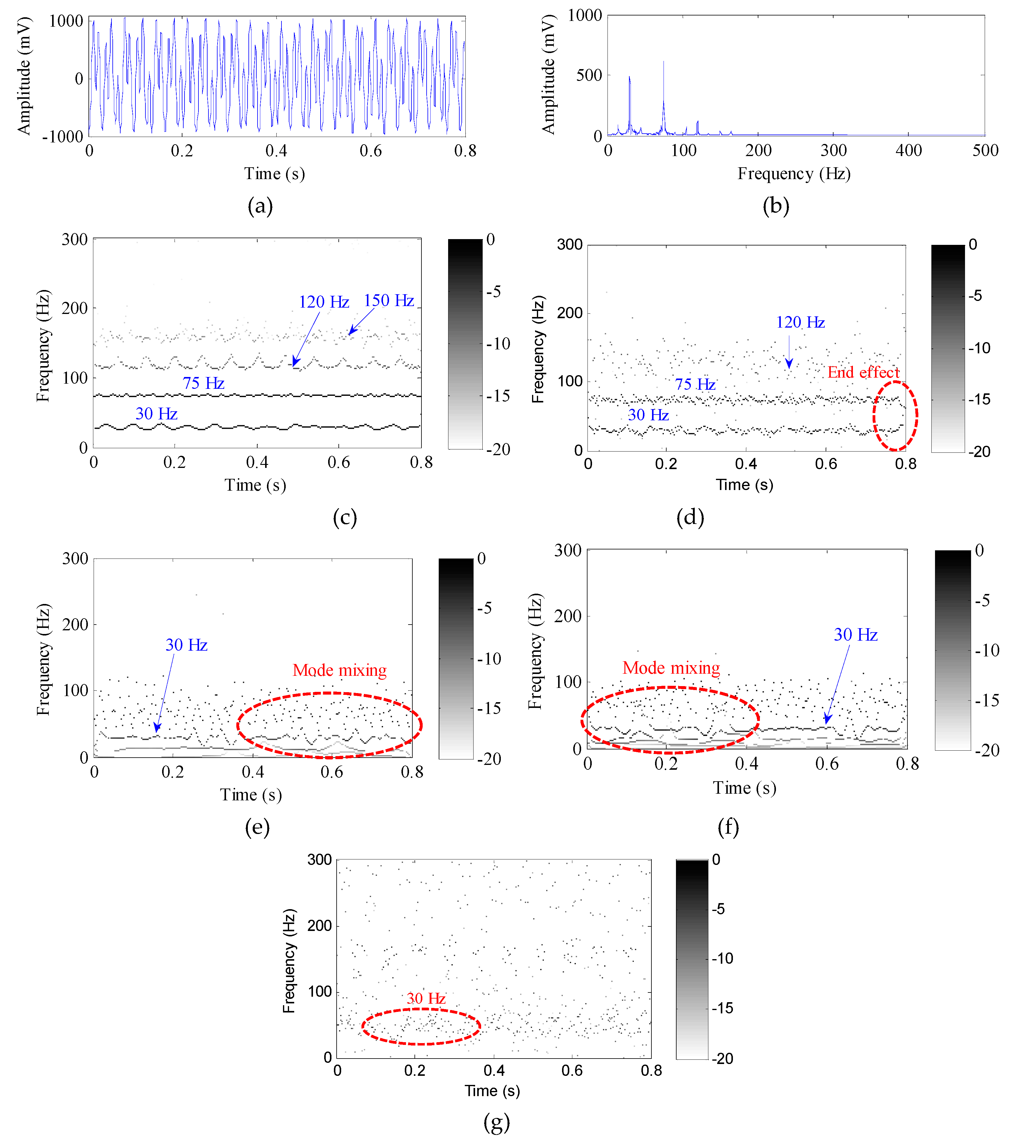
Figure 20a,b shows the waveform and FFT spectrum of the rotor oil-whip signal with a length of 1024, respectively. As depicted in Figure 20b, the oil-whip frequency $f_w$ of 30 Hz and rotating frequency $f_w$ of 75 Hz can be clearly seen in the FFT spectrum, but the amplitudes at a high frequency are weak. Besides, the FFT spectrum is short of time-varying frequency contents.

Analogously, five methods (i.e., IAVMD, OVMD, LMD, EMD, and WT) are utilized to deal with the oil-whip signal. Figure 20c–g plots, respectively, the TFR obtained by the five methods. The inside parameters ($\widehat{\alpha }$ = 1987 and K = 4) of IAVMD are determined by using GWO. Two key parameters of OVMD are determined as $\widehat{\alpha }$ = 1175 and K = 4 by using PSO. As shown in Figure 20c, the oil-whip frequency (i.e., $f_w$ = 30 Hz) and rotating frequency (i.e., $f_3$ = 75 Hz) are very obvious. Moreover, the associated frequency components 120 Hz (i.e., $f_3$ + 1.5 $f_w$) and 150 Hz (i.e., 2 $f_3$) are also extracted, and the aggregation along the time-frequency trajectory is very explicit. This indicates that the oil-whip fault can be detected accurately by using the proposed method. As shown in Figure 20d, only three frequencies (i.e., $f_w$ = 30 Hz, $f_3$ = 75 Hz, and the relevant frequency 120 Hz) can be found, but the harmonic frequency of 150 Hz is almost invisible due to the discrete distribution of high frequency points. Besides, there is an end effect problem in Figure 20d. Seen from Figure 20e,f, the TFR derived from LMD and EMD can also extract the oil-whip frequency $f_w$ = 30 Hz, but the mode mixing phenomenon is very serious, and the time-frequency trajectory at higher frequency is discrete and blurry. The oil-whip frequency $f_w$ = 30 Hz can be seen in Figure 20g, but the resolution of the WT-based TFR is worse than that in our approach. Hence, according to the above comparison results, compared with the other methods, our approach is more effective for detecting rotor oil-whip. In short, we can know from Figure 18, Figure 19 and Figure 20 that the proposed method is once again validated as being valuable in analyzing multi-component signals.

5.5. Result and Discussion

As analyzed above, the presented approach is applicable to processing multi-component signals and is more effective than the existing methods (i.e., OVMD, LMD, EMD, and WT) in extracting time-frequency contents and fault features. The advantage of merging several procedures (i.e., waveform matching extension, GWO, VMD, and TEO) is that it makes the resulting algorithm more adaptive to the practical situation and that it can directly extract time-varying characteristics. Besides, the presented approach can improve the precision of signal decomposition. However, the above results are geared to qualitative analysis, which indicates that a quantitative analysis should also be conducted to further show the performance of the proposed method. Here, three evaluation indexes (i.e., the energy error $\theta$, orthogonal index $OI$, and correlation coefficient shown in Equation (11)) are adopted to compare, on a quantificational level, the decomposability of different methods.

The energy error $\theta$ of one signal $x(t)$ can be given by [58]:

$$\theta =\frac{\left|\sqrt{{\displaystyle \sum _{i=1}^{n+1}RM{S}_i^2}}-RM{S}_x\right|}{RM{S}_x},RM{S}_x=\sqrt{\frac{{\displaystyle \sum _{i=1}^N{x}^2(i)}}{N}}$$

(20)

where $RM{S}_x$ represents the root mean square of $x(t)$, $RM{S}_i$ represents the root mean square of the i-th modes, and n + 1 represents the mode number. According to Ref. [58], the smaller $\theta$ value represents a higher decomposition accuracy and a lesser end effect.

The orthogonal index of one signal $x(t)$ can be given by [59]:

$$OI=\frac{{\displaystyle {\sum }_{i=1}^{N_C}{\displaystyle {\sum }_{j=1}^{j<i}\left|{\displaystyle {\sum }_{k=1}^N{C}_{ik}\times C_{jk}}\right|}}}{{\displaystyle {\sum }_{k=1}^N{(x_k-r_k)}^2}}$$

(21)

where $N_C$ represents the mode number, N means the data length of modes, $C_{ik}(t)$ and $C_{jk}(t)$ respectively denote the i-th and j-th modes at the sifting step k, and $x_k$ and $r_k$ denote the raw signal and residual term, respectively. Similarly, according to Ref. [59], the smaller the value of the orthogonal index is, the better the decomposition performance is. Furthermore, it should be explained that we evaluate their performance through calculating the correlation coefficient between the raw signal with the signals reconstructed by different methods.

Table 2. The quantitative comparisons among different approaches in the simulation signal.

Methods	$\mathbf{Energy}\mathbf{Error}\mathit{\theta }$		$\mathbf{Orthogonal}\mathbf{Index}\mathit{O}\mathit{I}$		Computing Time (s)
	Case 1	Case 2	Case 1	Case 2	Case 1	Case 2
IAVMD	0.0147	0.0151	0.0045	0.0048	56.7163	43.1932
OVMD	0.0231	0.0209	0.0113	0.0126	32.4437	26.9957
LMD	0.0409	0.0348	0.0304	0.0416	3.5421	3.8951
EMD	0.0992	0.1053	0.0612	0.0585	3.2879	3.0517
WT	0.0394	0.0572	0.0365	0.0403	2.3585	2.7138

,

Table 3. The quantitative comparisons among different approaches in the experiment signal.

Methods	$\mathbf{Energy}\mathbf{Error}\mathit{\theta }$			$\mathbf{Orthogonal}\mathbf{Index}\mathit{O}\mathit{I}$			Computing Time (s)
	Case 1	Case 2	Case 3	Case 1	Case 2	Case 3	Case 1	Case 2	Case 3
IAVMD	0.0209	0.0174	0.0158	0.0034	0.0060	0.0054	32.0132	27.0215	24.9027
OVMD	0.0238	0.0221	0.0253	0.0213	0.0133	0.0228	20.1082	16.8875	15.5641
LMD	0.0273	0.0198	0.0169	0.0672	0.0195	0.0201	1.9617	2.8573	2.9322
EMD	0.0319	0.0295	0.0703	0.0948	0.0602	0.0430	1.7810	2.6301	2.7835
WT	0.0563	0.0702	0.0681	0.0513	0.0303	0.0448	1.3016	1.5158	1.6914

and

Table 4. The correlation coefficient among different approaches in the simulation and experiment signal.

Methods	Correlation Coefficient of Simulation		Correlation Coefficient of Experiment
	Case 1	Case 2	Case 1	Case 2	Case 3
IAVMD	1.0000	0.9989	1.0000	0.9999	0.9999
OVMD	0.9996	0.9925	0.9998	0.9992	0.9993
LMD	0.9968	0.9897	0.9838	0.9985	0.9976
EMD	0.9908	0.9888	0.9830	0.9878	0.9901
WT	0.7989	0.8751	0.7291	0.7656	0.8586

list the energy error $\theta$, orthogonal index $OI$, and correlation coefficient of the decomposition results obtained by different approaches for the simulation data and experimental signal, respectively. It can be known from Table 2 and Table 3 that two evaluation indexes ($\theta$ and $OI$) of our proposed IAVMD approach are lower than those in four similar approaches (i.e., OVMD, LMD, EMD, and WT), which implies that our approach is equipped with satisfactory a decomposition performance in analyzing complicated compound signals compared with other similar methods (i.e., OVMD, LMD, EMD, and WT). However, it should be pointed out that the computational load of our approach is greater than those in other methods (i.e., OVMD, LMD, EMD, and WT) because of the waveform matching and parameter optimization procedure. Besides, OVMD also has a high computation time including the time cost of two stages (i.e., parameter optimization and signal decomposition). Hence, with the help of the high-end computing platform and computer technology, the improvement of the calculation efficiency of the proposed approach is regarded as our following work and research direction. Besides, as shown in Table 4, the correlation coefficient of our presented approach is greater than those in four similar approaches, which indicates that our presented approach is equipped with a lesser reconstruction error and a better decomposition performance compared with some typical techniques mentioned in the study.

To compare the decomposability of different methods more intuitively and quantify the time/memory costs of different methods more precisely, we add the percentage differences of the IAVMD method with respect to the others (OVMD, LMD, EMD, and WT).

Table 5. The percentage differences of the IAVMD with respect to other approaches in the simulation signal.

Method Comparison	$\mathbf{Energy}\mathbf{Error}\mathit{\theta }$		$\mathbf{Orthogonal}\mathbf{Index}\mathit{O}\mathit{I}$
	Case 1	Case 2	Case 1	Case 2
IAVMD vs. OVMD	0.84% ↓	0.58% ↓	0.68% ↓	0.78% ↓
IAVMD vs. LMD	2.62% ↓	1.97% ↓	2.59% ↓	3.68% ↓
IAVMD vs. EMD	8.45% ↓	9.02% ↓	5.67% ↓	5.37% ↓
IAVMD vs. WT	2.47% ↓	4.21% ↓	3.20% ↓	3.55% ↓

Where ↓ denotes the symbol of the reduced percentage.

and

Table 6. The percentage differences of the IAVMD with respect to other approaches in the experiment signal.

Methods	$\mathbf{Energy}\mathbf{Error}\mathit{\theta }$			$\mathbf{Orthogonal}\mathbf{Index}\mathit{O}\mathit{I}$
	Case 1	Case 2	Case 3	Case 1	Case 2	Case 3
IAVMD vs. OVMD	0.29% ↓	0.47% ↓	0.95% ↓	1.79% ↓	0.73% ↓	1.74% ↓
IAVMD vs. LMD	0.64% ↓	0.24% ↓	0.11% ↓	6.38% ↓	1.35% ↓	1.47% ↓
IAVMD vs. EMD	1.10% ↓	1.21% ↓	5.45% ↓	9.14% ↓	5.42% ↓	3.76% ↓
IAVMD vs. WT	3.54% ↓	5.28% ↓	5.23% ↓	4.79% ↓	2.43% ↓	3.94% ↓

Where ↓ denotes the symbol of the reduced percentage.

list the percentage differences between the IAVMD and other approaches in the simulation and experiment signal, respectively. It can be seen from Table 5 and Table 6 that the index value (energy error $\theta$ and orthogonal index $OI$) of the IAVMD method is reduced compared with the other approaches (OVMD, LMD, EMD, and WT). The smallest percentage difference of IAVMD is about 0.1%, but the largest percentage difference can reach 9%. This indicates that the proposed IAVMD method has a certain degree of advantage in signal decomposition. However, at present, the significance of quantification of this small degree is still undetermined, which is the focus of our future research.

Table 7. Assessment of the time and memory cost of different approaches.

Methods	Memory of Simulation (KByte)		Memory of Experiment (KByte)			Average Time (s)
	Case 1	Case 2	Case 1	Case 2	Case 3
IAVMD	8.85	8.87	8.91	8.92	8.91	36.76→High
OVMD	5.46	5.48	5.04	5.03	5.03	28.67→High
LMD	1.93	1.96	1.98	1.97	1.98	3.04→Low
EMD	1.71	1.73	1.75	1.76	1.76	2.27→Low
WT	1.35	1.38	1.41	1.41	1.42	1.92→Low

lists the memory cost and average time of different methods. Note that the memory cost of different methods is measured based on the memory usage of the MATLAB file of different methods. As shown in Table 7, the memory cost of IAVMD is the highest (above 8 Kbyte), the second biggest memory cost is the OVMD method, and WT has the smallest memory cost (i.e., the average cost is 1.39 Kbyte). In addition, the average time costs of our method and OVMD are high (above 25 s), whereas the other three methods (LMD, EMD, and WT)) have low time costs which are under 4 s.

In a word, by observing the frequency components of the time-frequency representations, we can find that the IAVMD method can excavate a better and more accurate frequency content compared with other approaches (OVMD, LMD, EMD, and WT). Besides, through the above quantification, we can draw the conclusion that the IAVMD method can improve the decomposition precision of the signal to some extent, but that it also brings about an additional computational cost due to an increased preparation stage. If one wants to extend the proposed IAVMD method to the practical engineering application, its time cost needs to be decreased, which is also the focus of our future study.

6. Conclusions

In this article, to solve the shortcoming of the subjective parameter selection and end effect phenomenon existing in the original VMD, a novel time-frequency analysis tool (i.e., IAVMD) consisting of waveform matching extension, GWO-based parameter optimization, and TEO demodulation is presented, which can automatically determine the inside parameters ($\widehat{\alpha }$, K) of VMD and separate a non-stationary compound signal into a superposition of modes. Several simulated data and experimental examples are provided to validate the effectiveness of our approach. Studies confirm that our approach can effectively identify fault features related to rotor early rub-impact, oil-whirl, and oil-whip. Besides, our proposed method outperforms four available approaches (i.e., OVMD, LMD, EMD, and WT) in analyzing the non-stationary compound signal with multi-frequency contents. The novelties and attractions of this paper are as follows:

(1) The concept of waveform matching extension is introduced to alleviate the end effect problem in the traditional VMD method.

(2) A novel time-frequency analysis algorithm termed as IAVMD is presented, which can avoid the effective manual parameter selection and improve diagnostic accuracy.

(3) The efficacy of our method is demonstrated through the simulated and experimental data.

Our future direction will focus on extending the proposed method to analyze multi-component signals in practical applications. Moreover, in our future work, fault diagnosis analyses under variable speeds will also be investigated by using the presented approach. Finally, in the follow-up work, the availability of our presented approach will be discussed in detail when strong noise and more interference are appended to the analyzed vibration signal.

References

- Lei, Y.; Lin, J.; He, Z.; Zuo, M.J.; Zuo, M. A review on empirical mode decomposition in fault diagnosis of rotating machinery. Mech. Syst. Signal. Process. 2013, 35, 108–126. [Google Scholar] [CrossRef]
- Zhang, F.; Huang, J.; Chu, F.; Cui, L. Mechanism and Method for Outer Raceway Defect Localization of Ball Bearings. IEEE Access 2020, 8, 4351–4360. [Google Scholar] [CrossRef]
- Yan, X.; Liu, Y.; Jia, M. Research on an enhanced scale morphological-hat product filtering in incipient fault detection of rolling element bearings. Measurement 2019, 147, 106856. [Google Scholar] [CrossRef]
- Yu, K.; Lin, T.R.; Ma, H.; Li, H.; Zeng, J. A combined polynomial chirplet transform and synchroextracting technique for analyzing nonstationary signals of rotating machinery. IEEE Trans. Instrum. Meas. 2019, 1. [Google Scholar] [CrossRef]
- Feng, Z.; Liang, M.; Chu, F. Recent advances in time–frequency analysis methods for machinery fault diagnosis: A review with application examples. Mech. Syst. Signal. Process. 2013, 38, 165–205. [Google Scholar] [CrossRef]
- Yan, S.; Nguang, S.K.; Zhang, L. Nonfragile Integral-Based Event-Triggered Control of Uncertain Cyber-Physical Systems under Cyber-Attacks. Complexity 2019, 2019, 1–14. [Google Scholar] [CrossRef]
- Huang, Y.; Lu, R.; Chen, K. Detection of internal defect of apples by a multichannel Vis/NIR spectroscopic system. Postharvest Biol. Technol. 2020, 161, 111065. [Google Scholar] [CrossRef]
- Yan, R.; Gao, R.X.; Chen, X. Wavelets for fault diagnosis of rotary machines: A review with applications. Signal. Process. 2014, 96, 1–15. [Google Scholar] [CrossRef]
- Yan, X.; Liu, Y.; Jia, M. Multiscale cascading deep belief network for fault identification of rotating machinery under various working conditions. Knowl. Based Syst. 2020. [Google Scholar] [CrossRef]
- Guo, W.; Tse, P.W.T.; Djordjevich, A. Faulty bearing signal recovery from large noise using a hybrid method based on spectral kurtosis and ensemble empirical mode decomposition. Measurement 2012, 45, 1308–1322. [Google Scholar] [CrossRef]
- Xiang, L.; Yan, X. A self-adaptive time-frequency analysis method based on local mean decomposition and its application in defect diagnosis. J. Vib. Control 2016, 22, 1049–1061. [Google Scholar] [CrossRef]
- Yan, X.; Liu, Y.; Jia, M. A Feature Selection Framework-Based Multiscale Morphological Analysis Algorithm for Fault Diagnosis of Rolling Element Bearing. IEEE Access 2019, 7, 123436–123452. [Google Scholar] [CrossRef]
- Li, Y.; Xu, M.; Wei, Y.; Huang, W. Rotating machine fault diagnosis based on intrinsic characteristic-scale decomposition. Mech. Mach. Theory 2015, 94, 9–27. [Google Scholar] [CrossRef]
- Dragomiretskiy, K.; Zosso, D. Variational Mode Decomposition. IEEE Trans. Signal. Process. 2013, 62, 531–544. [Google Scholar] [CrossRef]
- Upadhyay, A.; Sharma, M.; Pachori, R.B. Determination of instantaneous fundamental frequency of speech signals using variational mode decomposition. Comput. Electr. Eng. 2017, 62, 630–647. [Google Scholar] [CrossRef]
- Lahmiri, S.; Shmuel, A. Variational mode decomposition based approach for accurate classification of color fundus images with hemorrhages. Opt. Laser Technol. 2017, 96, 243–248. [Google Scholar] [CrossRef]
- Xue, Y.-J.; Cao, J.-X.; Wang, D.-X.; Du, H.-K.; Yao, Y. Application of the Variational-Mode Decomposition for Seismic Time–frequency Analysis. IEEE J. Sel. Top. Appl. Earth Obs. Remote. Sens. 2016, 9, 3821–3831. [Google Scholar] [CrossRef]
- Jiang, X.; Wang, J.; Shi, J.; Shen, C.; Huang, W.; Zhu, Z. A coarse-to-fine decomposing strategy of VMD for extraction of weak repetitive transients in fault diagnosis of rotating machines. Mech. Syst. Signal. Process. 2019, 116, 668–692. [Google Scholar] [CrossRef]
- Wang, D.; Luo, H.; Grunder, O.; Lin, Y. Multi-step ahead wind speed forecasting using an improved wavelet neural network combining variational mode decomposition and phase space reconstruction. Renew. Energy 2017, 113, 1345–1358. [Google Scholar] [CrossRef]
- Liu, H.; Mi, X.; Li, Y. Smart multi-step deep learning model for wind speed forecasting based on variational mode decomposition, singular spectrum analysis, LSTM network and ELM. Energy Convers. Manag. 2018, 159, 54–64. [Google Scholar] [CrossRef]
- Upadhyay, A.; Pachori, R.B. Instantaneous voiced/non-voiced detection in speech signals based on variational mode decomposition. J. Frankl. Inst. 2015, 352, 2679–2707. [Google Scholar] [CrossRef]
- Upadhyay, A.; Pachori, R. Speech enhancement based on mEMD-VMD method. Electron. Lett. 2017, 53, 502–504. [Google Scholar] [CrossRef]
- An, X.; Pan, L.; Zhang, F. Analysis of hydropower unit vibration signals based on variational mode decomposition. J. Vib. Control 2017, 23, 1938–1953. [Google Scholar] [CrossRef]
- Wang, Y.; Markert, R.; Xiang, J.; Zheng, W. Research on variational mode decomposition and its application in detecting rub-impact fault of the rotor system. Mech. Syst. Signal. Process. 2015, 60, 243–251. [Google Scholar] [CrossRef]
- Yang, W.; Peng, Z.; Wei, K.; Shi, P.; Tian, W. Superiorities of variational mode decomposition over empirical mode decomposition particularly in time–frequency feature extraction and wind turbine condition monitoring. Iet Renew. Power Gener. 2016, 11, 443–452. [Google Scholar] [CrossRef] [Green Version]
- Yao, J.; Xiang, Y.; Qian, S.; Wang, S.; Wu, S. Noise source identification of diesel engine based on variational mode decomposition and robust independent component analysis. Appl. Acoust. 2017, 116, 184–194. [Google Scholar] [CrossRef]
- Zhang, M.; Jiang, Z.; Feng, K. Research on variational mode decomposition in rolling bearings fault diagnosis of the multistage centrifugal pump. Mech. Syst. Signal. Process. 2017, 93, 460–493. [Google Scholar] [CrossRef] [Green Version]
- Liu, H.; Xiang, J. A Strategy Using Variational Mode Decomposition, L-Kurtosis and Minimum Entropy Deconvolution to Detect Mechanical Faults. IEEE Access 2019, 7, 70564–70573. [Google Scholar] [CrossRef]
- Isham, M.F.; Leong, M.S.; Lim, M.H.; Ahmad, Z.A. Variational mode decomposition: Mode determination method for rotating machinery diagnosis. J. Vibroeng. 2018, 20, 2604–2621. [Google Scholar] [CrossRef] [Green Version]
- Yang, H.; Liu, S.; Zhang, H. Adaptive estimation of VMD modes number based on cross correlation coefficient. J. Vibroeng. 2017, 19, 1185–1196. [Google Scholar] [CrossRef]
- Liu, Y.; Yang, G.; Li, M.; Yin, H. Variational mode decomposition denoising combined the detrended fluctuation analysis. Signal. Process. 2016, 125, 349–364. [Google Scholar] [CrossRef]
- Jiang, F.; Zhu, Z.; Li, W. An Improved VMD With Empirical Mode Decomposition and Its Application in Incipient Fault Detection of Rolling Bearing. IEEE Access 2018, 6, 44483–44493. [Google Scholar] [CrossRef]
- Zhang, J.; He, J.; Long, J.; Yao, M.; Zhou, W. A New Denoising Method for UHF PD Signals Using Adaptive VMD and SSA-Based Shrinkage Method. Sensors 2019, 19, 1594. [Google Scholar] [CrossRef] [Green Version]
- Li, Z.; Chen, J.; Zi, Y.; Pan, J. Independence-oriented VMD to identify fault feature for wheel set bearing fault diagnosis of high speed locomotive. Mech. Syst. Signal. Process. 2017, 85, 512–529. [Google Scholar] [CrossRef]
- Zhao, C.; Feng, Z. Application of multi-domain sparse features for fault identification of planetary gearbox. Measurement 2017, 104, 169–179. [Google Scholar] [CrossRef]
- Wang, Z.; Wang, J.; Du, W. Research on Fault Diagnosis of Gearbox with Improved Variational Mode Decomposition. Sensors 2018, 18, 3510. [Google Scholar] [CrossRef] [Green Version]
- Lian, J.; Liu, Z.; Wang, H.; Dong, X. Adaptive variational mode decomposition method for signal processing based on mode characteristic. Mech. Syst. Signal Process. 2018, 107, 53–77. [Google Scholar] [CrossRef]
- Shan, Y.; Zhou, J.; Jiang, W.; Liu, J.; Xu, Y.; Zhao, Y. A fault diagnosis method for rotating machinery based on improved variational mode decomposition and a hybrid artificial sheep algorithm. Meas. Sci. Technol. 2019, 30, 055002. [Google Scholar] [CrossRef]
- Isham, M.F.; Leong, M.S.; Lim, M.H.; Bin Ahmad, Z.A. Intelligent wind turbine gearbox diagnosis using VMDEA and ELM. Wind Energy 2019, 22, 813–833. [Google Scholar] [CrossRef]
- Zhu, J.; Wang, C.; Hu, Z.; Kong, F.; Liu, X. Adaptive variational mode decomposition based on artificial fish swarm algorithm for fault diagnosis of rolling bearings. Proc. Inst. Mech. Eng. Part. C J. Mech. Eng. Sci. 2017, 231, 635–654. [Google Scholar] [CrossRef]
- Yi, C.; Lv, Y.; Dang, Z. A Fault Diagnosis Scheme for Rolling Bearing Based on Particle Swarm Optimization in Variational Mode Decomposition. Shock. Vib. 2016, 2016, 1–10. [Google Scholar] [CrossRef] [Green Version]
- Yan, X.; Jia, M. Application of CSA-VMD and optimal scale morphological slice bispectrum in enhancing outer race fault detection of rolling element bearings. Mech. Syst. Signal Process. 2019, 122, 56–86. [Google Scholar] [CrossRef]
- Wang, Z.; He, G.; Du, W.; Zhou, J.; Han, X.; Wang, J.; He, H.; Guo, X.; Wang, J.; Kou, Y. Application of Parameter Optimized Variational Mode Decomposition Method in Fault Diagnosis of Gearbox. IEEE Access 2019, 7, 44871–44882. [Google Scholar] [CrossRef]
- Zhou, J.; Guo, X.; Du, W.; Han, X.; Wang, J.; He, H.; Xue, H.; Kou, Y.; Zhou, J.; Guo, X. Research on Fault Extraction Method of Variational Mode Decomposition Based on Immunized Fruit Fly Optimization Algorithm. Entropy 2019, 21, 400. [Google Scholar] [CrossRef] [Green Version]
- Wei, D.; Jiang, H.; Shao, H.; Li, X.; Lin, Y. An optimal variational mode decomposition for rolling bearing fault feature extraction. Meas. Sci. Technol. 2019, 30, 055004. [Google Scholar] [CrossRef]
- Miao, Y.; Zhao, M.; Lin, J. Identification of mechanical compound-fault based on the improved parameter-adaptive variational mode decomposition. Isa Trans. 2019, 84, 82–95. [Google Scholar] [CrossRef] [PubMed]
- Mirjalili, S.; Mirjalili, S.M.; Lewis, A. Grey wolf optimizer. Adv. Eng. Softw. 2014, 69, 46–61. [Google Scholar] [CrossRef] [Green Version]
- Yan, X.; Jia, M. A novel optimized SVM classification algorithm with multi-domain feature and its application to fault diagnosis of rolling bearing. Neurocomputing 2018, 313, 47–64. [Google Scholar] [CrossRef]
- Yan, X.; Liu, Y.; Jia, M. Health condition identification for rolling bearing using a multi-domain indicator-based optimized stacked denoising autoencoder. Struct. Health Monit. 2019, 1475921719893594. [Google Scholar] [CrossRef]
- He, W.; Jiang, Z.-N.; Feng, K. Bearing fault detection based on optimal wavelet filter and sparse code shrinkage. Measurement 2009, 42, 1092–1102. [Google Scholar] [CrossRef]
- Li, C.; Zhou, J. Semi-supervised weighted kernel clustering based on gravitational search for fault diagnosis. Isa Trans. 2014, 53, 1534–1543. [Google Scholar] [CrossRef] [PubMed]
- Zhang, X.; Miao, Q.; Liu, Z.; He, Z. An adaptive stochastic resonance method based on grey wolf optimizer algorithm and its application to machinery fault diagnosis. Isa Trans. 2017, 71, 206–214. [Google Scholar] [CrossRef] [PubMed]
- Hu, A. New process method for end effects of HILBERT-HUANG transform. Chin. J. Mech. Eng. 2008, 44, 154. [Google Scholar] [CrossRef]
- Rodríguez, P.H.; Alonso, J.B.; Ferrer, M.A.; Travieso, C.M.; Alonso-Hernández, J.B.; Travieso-González, C.M. Application of the Teager–Kaiser energy operator in bearing fault diagnosis. Isa Trans. 2013, 52, 278–284. [Google Scholar] [CrossRef] [PubMed]
- Yan, X.; Liu, Y.; Jia, M.; Zhu, Y. A Multi-Stage Hybrid Fault Diagnosis Approach for Rolling Element Bearing Under Various Working Conditions. IEEE Access 2019, 7, 138426–138441. [Google Scholar] [CrossRef]
- Yan, X.; Jia, M. Improved singular spectrum decomposition-based 1.5-dimensional energy spectrum for rotating machinery fault diagnosis. J. Braz. Soc. Mech. Sci. Eng. 2019, 41, 50. [Google Scholar] [CrossRef]
- Zhang, X.; Miao, Q.; Zhang, H.; Wang, L. A parameter-adaptive VMD method based on grasshopper optimization algorithm to analyze vibration signals from rotating machinery. Mech. Syst. Signal Process. 2018, 108, 58–72. [Google Scholar] [CrossRef]
- Hu, A.; Yan, X.; Xiang, L. A new wind turbine fault diagnosis method based on ensemble intrinsic time-scale decomposition and WPT-fractal dimension. Renew. Energy 2015, 83, 767–778. [Google Scholar] [CrossRef]
- Peel, M.; Pegram, G.; McMahon, T. Empirical mode decomposition: Improvement and application. Proc. Int. Congr. Model. Simul. 2007, 1, 2996–3002. [Google Scholar]
Figure 1.
Flowchart of the waveform matching extension.
Figure 2.
Sketch map of the waveform matching extension.
Figure 3.
Intuitive examples of the waveform matching extension: (a) a cycle shock pulse signal and (b) a modulated compound signal.
Figure 4.
The time domain waveform of the simulation signal: (a) No outlier, (b) single outlier, and (c) multiple outlier.
Figure 5.
A population hierarchy of the GWO algorithm.
Figure 6.
Flowchart of the parameter optimization of VMD using the GWO algorithm.
Figure 7.
The flowchart of the proposed IAVMD method.
Figure 8.
The numerical signal y(t) and its FFT spectrum.
Figure 9.
The decomposition results obtained by IAVMD for simulation 1 and their corresponding FFT spectrum.
Figure 10.
The time-frequency representations obtained by IAVMD for simulation 1: (a) Two-dimensional and (b) three-dimensional.
Figure 11.
The decomposition results obtained by different methods for simulation 1: (a) VMD, (b) LMD, (c) EMD, and (d) WT.
Figure 12.
The time-frequency representations obtained by different methods for simulation 1: (a) OVMD, (b) LMD, (c) EMD, and (d) WT.
Figure 13.
The numerical signal and its FFT spectrum.
Figure 14.
The decomposition results obtained by IAVMD for simulation 2 and their corresponding FFT spectrum.
Figure 15.
The time-frequency representations obtained by IAVMD for simulation 2: (a) Two-dimensional and (b) three-dimensional.
Figure 16.
The time-frequency representations obtained by different methods for simulation 2: (a) OVMD, (b) LMD, (c) EMD, and (d) WT.
Figure 17.
Schematic diagram of the rotor test bench.
Figure 18.
The analyzed results of the rotor rub-impact signal: (a) Temporal waveform, (b) FFT spectrum, time-frequency representations obtained by (c) IAVMD, (d) OVMD, (e) LMD, (f) EMD, and (g) WT.
Figure 19.
The analyzed results of the rotor oil-whirl signal: (a) Temporal waveform, (b) FFT spectrum, time-frequency representations obtained by (c) IAVMD, (d) OVMD, (e) LMD, (f) EMD, and (g) WT.
Figure 20.
The analyzed results of the rotor oil-whip signal: (a) Temporal waveform, (b) FFT spectrum, time-frequency representations obtained by (c) IAVMD, (d) OVMD, (e) LMD, (f) EMD, and (g) WT.