Convolutional Neural Networks Using Skip Connections with Layer Groups for Super-Resolution Image Reconstruction Based on Deep Learning


Intelligent Image Processing Laboratory, Konkuk University, Seoul 05029, Korea
*
Author to whom correspondence should be addressed.
Appl. Sci. 2020, 10(6), 1959; https://0-doi-org.brum.beds.ac.uk/10.3390/app10061959
Submission received: 12 February 2020
/
Revised: 7 March 2020
/
Accepted: 10 March 2020
/
Published: 13 March 2020
(This article belongs to the Section Computing and Artificial Intelligence)
Abstract
:In this paper, we propose a deep learning method with convolutional neural networks (CNNs) using skip connections with layer groups for super-resolution image reconstruction. In the proposed method, entire CNN layers for residual data processing are divided into several layer groups, and skip connections with different multiplication factors are applied from input data to these layer groups. With the proposed method, the processed data in hidden layer units tend to be distributed in a wider range. Consequently, the feature information from input data is transmitted to the output more robustly. Experimental results show that the proposed method yields a higher peak signal-to-noise ratio and better subjective quality than existing methods for super-resolution image reconstruction.
1. Introduction
Single image super-resolution (SISR) is a method to reconstruct a super-resolution image from a single low-resolution image [1,2]. The reconstruction of a super-resolution image is generally difficult because of various issues, such as blur and noise. Image processing methods such as interpolation were developed for this purpose before the advent of deep learning. Many applications are based on deep learning in the image processing and computer vision field [1,2,3,4].
The first solution for super-resolution reconstruction from a low-resolution image using deep learning with convolutional neural networks (CNNs) was the super-resolution convolutional neural network (SRCNN) method [1]. However, in the SRCNN method, learning was not performed well in deep layers. The very deep super-resolution (VDSR) method [2] is more efficient for learning in deep layers and achieves better performance than SRCNN for super-resolution reconstruction. Although VDSR has layers much deeper than those in SRCNN, it is efficient because it focuses on generating only residual (high-frequency) information by connecting the input data to the output of the last layer with a skip connection. However, in the VDSR method, the gradient information vanishes, owing to repeated rectified linear unit (ReLU) operations. It was observed that the number of hidden data units with vanishing gradients increases as the training proceeds with many iterations [5]. To resolve the problem of gradient vanishing, batch normalization [6] can be applied, but it may cause data distortion and other negative effects for reconstructing super-resolution images.
The super-resolution image reconstruction performance of the VDSR method [2] is significantly better than that of SRCNN because it uses deep layers and a skip connection. The skip connection is applied only once between the input data and the output of the last layer in the existing VDSR method [2]. In the existing VDSR method, it is difficult to maintain the characteristics of the input data entering the neural network. In each layer, a ReLU operation is performed after a convolution operation.
The ReLU operation is defined as
where negative values are clipped to zero.
In VDSR, the data entering network layers would be residual-type with high-frequency components. Approximately half of the output values of the convolution operation are negative in each layer. Because negative values are clipped to zero, approximately half of the output values of ReLU are zero. The remaining positive values after ReLU operation are redistributed into positive and negative values through the convolution operation in the next layer. As the epoch with many iterations proceeds, the percentage of zero and small (close to zero) values increases in the output data of ReLU in each layer, which causes serious extinction of the information used in the learning for reconstruction. This would be the reason for the problem of gradient vanishing after repeated ReLU operations for residual-type data.
Figure 1 shows the network structure of VDSR. In the figure, denotes the whole layer group, which is composed of l layers ( in Figure 1). The layer group performs whole operations on residual data. Each layer block performs a convolution operation and a ReLU activation function operation. In VDSR, the multiplication factor (MF) for the skip connection is fixed as 1.0.
Let represent the function of the layer group . When a low-resolution image is the input data for the neural network, the operation result of the layer group in VDSR can be expressed as ). The output data , which is the super-resolution image, can be expressed as follows:
Skip connections have been used in other residual-type networks [7,8]. He et al. used a skip connection within a building block of residual network (ResNet) [7]. The MF for the skip connection is fixed as 1 for identity connection. One building block is composed of two convolution layers and two ReLU operations. These building blocks are concatenated serially for the whole ResNet. Hence, the data processed by a building block are transferred to the next building block, but the original input data are not transferred to most building blocks. ResNet was developed for image recognition [7].
In [8], skip connections are applied for residual function blocks. There is a fixed scaling (multiplication) factor for each residual function block. The output of residual function is multiplied by this scaling factor, whereas the input is not multiplied by this scaling factor. The data processed by the residual function are added to the input data, and the added data are transferred to the next residual function block. Hence, the original input data are not connected directly to the output of most residual function blocks. The structure in [8] was developed for selective pruning of the unimportant parts of CNNs rather than image reconstruction.
In this paper, we propose a deep learning method with CNNs for reconstructing super-resolution images. The proposed method divides entire layers into several layer groups with skip connections. The proposed method is designed to resolve the problem of gradient vanishing by reducing the extinction of data in hidden layer units through skip connections from the input data to layer groups. Experimental results show that the proposed method yields better results than previous methods for super-resolution image reconstruction.
2. Proposed Method
In this section, we propose a deep learning method with CNNs for super-resolution image reconstruction. In the proposed method, the output of each layer group is connected to input data with a skip connection. Each skip connection has a multiplication factor (MF) with input data, which is a parameter that is also to be learned during the training process. Hence, the proposed method connects input data to layer groups through multiple skip connections at regular intervals, whereas the existing VDSR method utilizes only one skip connection.
If the input image data are repetitively skipped and connected to a predetermined number of layer groups, the problem of data extinction due to ReLU operation at the output of each layer would be significantly alleviated. The first advantage of skip connections with regular intervals is that the data processed in each layer group would retain the characteristics of the input data to be learned without loss of input data information by data extinction and gradient vanishing. This phenomenon has a positive effect on learning for super-resolution reconstruction because the number of contributing units for learning in the proposed method would be greater than that in the structure without repetitive skip connections. The second advantage is that repetitive skip connections to all layer groups would maintain the features of the input image to be learned more robustly. The neural network for super-resolution reconstruction aims to improve the image quality by generating the optimum high-frequency information from the input low-resolution image. The repetitive skip connections would be advantageous to preserving the features of the input image to be learned for super-resolution reconstruction.
In the proposed method, because the number of skip connections with input data is relatively large, the neural network may be overfitted as the epochs roll over during training. To transmit the information of the input data to be learned while preserving their characteristics, each skip connection is associated with an MF, which represents the weight for input data. The MF of the proposed method is a parameter that is also to be learned during the training process. The value of this parameter is to be learned like other parameters, such as filter kernels. We experimentally observed that the super-resolution image reconstruction performance is improved when the MFs are learned and set through the training process.
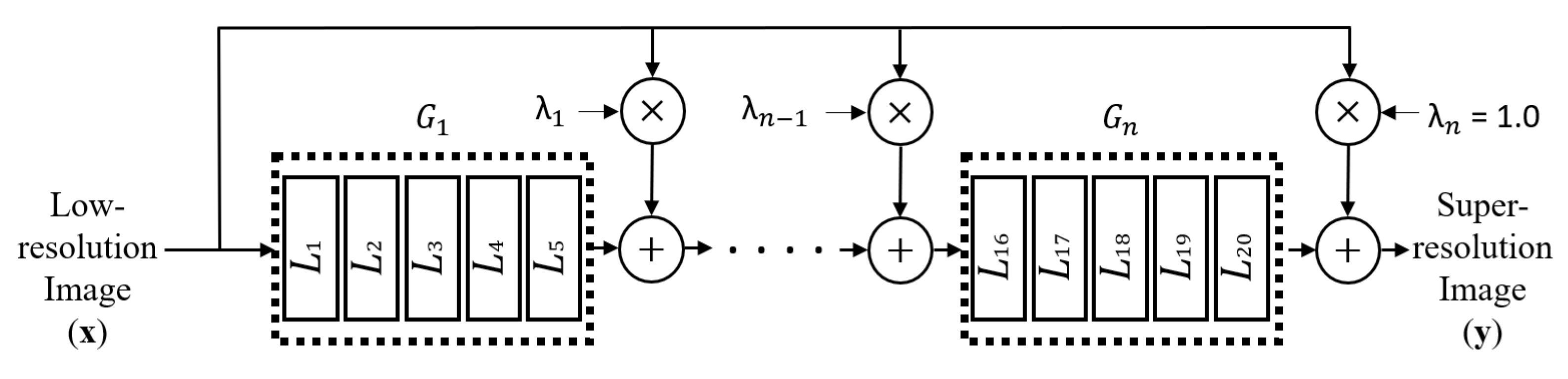
Figure 2 shows the proposed network structure with a different skip connection for each layer group. Let k represent the number of layers in a layer group and n represent the number of layer groups. The total number of layers l is given by . In Figure 2, () represents layer groups, each of which is composed of k layers.
Each represents the MF for layer group , and the last MF is fixed to 1.0 as in the existing VDSR method. The MF values of through are to be learned and updated as the optimization of parameters in the training process with initialization to some values.
Note that the structure of each in the proposed method (Figure 2) is the same as that of each in VDSR (Figure 1). Each in the proposed method is composed of one convolution layer and one ReLU layer as each in VDSR. There are 64 convolutions with filter kernels in one convolution layer. The parameters relating convolution operations in the proposed method are the same as the parameters relating convolution operations in VDSR. The operation of ReLU units in the proposed method is performed as (1), which is exactly the same as the VDSR.
The only different parameters are the MFs in the proposed method (Figure 2), which do not exist in the VDSR (Figure 1). The other differences are the skip connections for layer groups and the associated multiplications (represented as ⊗) and additions (represented as ⊕), as shown in Figure 2.
Let represent the function of layer group . The output of layer group is , and the input to the next layer group is . For the case of , , and , as shown in Figure 2, the relation among the input data , output data , and function of each layer group can be expressed as follows:
3. Results and Discussion
Experiments on the proposed method were performed using TensorFlow code on a computer with a 3.40 GHz Intel (R) Core (TM) i7-6700 CPU, 16 GB of memory, and an NVIDIA GeForce RTX 2080 graphics card. (The code and dataset are available at https://github.com/hg-a/MFVDSR.)
The training dataset includes 215,316 sub-images created by data argument with 291 images that combine images from image data reported by Yang et al. [9] and the Berkeley Segmentation Dataset [10]. Four datasets, namely, Set5, Set14, B100, and Urban100, were used as the test dataset for performance evaluation. The simulation results were compared with other super-resolution image reconstruction methods, such as A+ [11], SRCNN [1], and VDSR [2], by measuring the average peak signal-to-noise ratio (PSNR) for each test dataset. For the optimization of parameters in training, the Adam optimizer [12] was used for VDSR and the proposed method. In the proposed method, the k value was set to 2, 5, or 10, and different MFs were tested for various cases.
Table 1 presents a comparison of PSNR among the proposed method, A+ [11], SRCNN [1], and VDSR [2]. The A+ method performs super-resolution reconstruction using sparse dictionaries [11]. Table 1 shows that the PSNR performance of the proposed method, having repetitive skip connections with MFs for layer groups, is better than those of A+, SRCNN, and VDSR. Among A+, SRCNN, and VDSR, the VDSR method shows the best PSNR performance for all datasets. Experiments were conducted with different combinations of k, n, and values to find the optimal combination that yields the best performance.
The experimental results show that the proposed method shows the best PSNR performance when and . Each MF () value is initialized as 2.5 and optimized during the training process, while is fixed as 1.0. For the optimization of MF () values in training, Adam optimizer [12] is used and the learning rate (step size) is set as 0.0001.
For these datasets, the proposed method shows PSNR improvements of dB over the VDSR method. For scales , , and , the proposed method shows average PSNR improvements of 0.11, 0.08, and 0.06 dB, respectively, over the VDSR method.
Table 2 compares the PSNRs of the proposed method using different combinations of k, n, and . Fixed values are used in Case 1, Case 3, and Case 6. Meanwhile, in Case 2, Case 4, Case 5, and Case 7, some initial values are set for , and these values are learned and updated during the training process. The results in Table 2 indicate that the cases where is set to an initial value and updated during the training process show better results than the cases where is fixed. Hence, we argue that treating the MFs, , as parameters that are updated during the training process would result in improved performance with the proposed method. If we compare the results in terms of k and n, Case 3, Case 4, and Case 5 with and show better PSNR performances than the other cases.
In the case of and , as shown in Figure 2, there are four skip connections from input data to the output of four layer groups. Figure 3 and Figure 4 show the data distributions as histograms for data generated at the 60th epoch of the training process in layers , , and , which are the first layers of layer groups , , and , respectively. In the captions of Figure 3 and Figure 4, and denote the mean and standard deviation, respectively. Figure 3 shows a comparison of distributions for data generated before (as the input of) ReLU in VDSR and the proposed method, while Figure 4 shows a comparison of distributions for data generated after (as the output of) ReLU in VDSR and the proposed method. The comparison of Figure 3 and Figure 4 shows that negative values are clipped to zero, and the standard deviation significantly decreases after the ReLU operation for each case.
In Figure 4a–c, the repeated ReLU operations in VDSR force the data distribution to be concentrated in a very narrow range, and the values are small. Meanwhile, in Figure 4d–f, the repetitive skip connections from the input data to the layer groups in the proposed method result in data distributions in wider ranges, and the values are much larger than in the VDSR method. This effect increases the number of contributing data units for learning and maintains the features of the input image for super-resolution reconstruction more robustly. Therefore, the proposed method shows better super-resolution reconstruction performance than the VDSR method, even though it has the same number of layers.
Table 3 presents the comparison of training and test running time (sec) for SRCNN, VDSR, and the proposed method. The running time for training is very similar for VDSR and the proposed method. Since the network structure of SRCNN is relatively simple, the running times (per epoch and per 60 epochs) for training in SRCNN look smaller than VDSR and the proposed method. The running times for testing per image are very close for SRCNN, VDSR, and the proposed method.
Note that the loss value for training (or test PSNR value) converges at around 60 epochs for VDSR and the proposed method, whereas it does not converge at 60 epochs for SRCNN. For the training of SRCNN, 24,800 sub-images are used [1]. In experimental results in [1], the number of backpropagations should be at least (more than 20,000 epochs) for convergence in training for SRCNN. In our experiments for VDSR and the proposed method, 215,316 sub-images are used. To achieve more than backpropagations with 215,316 sub-images in training, it requires at least 2300 epochs in training. This means that it would require at least s for the convergence of training in SRCNN. Hence, SRCNN would require much more time for training than VDSR and the proposed method. If we compare the convergence time (per 60 epochs) for training, the proposed method takes slightly more time (by 1.3%) than VDSR. It is due to the extra time for the optimization of MF values and the associated multiplication and addition operations.
Figure 5, Figure 6 and Figure 7 show the results of super-resolution image reconstruction using VDSR and the proposed method from bicubic interpolated images with the scale factor . The bars on the right of Figure 5 are low-brightness straight objects arranged side by side at regular intervals. In the image reconstructed using VDSR, linear objects do not maintain their shape, while the proposed method maintains the linear shape well. In Figure 6, the proposed method shows better performance than VDSR in maintaining the pattern of the grid with the correct shape of the ceiling, where grids with high contrast are arranged regularly. Because the linear objects in the building in Figure 7 are very tightly spaced, the VDSR result is blurry and the straight lines are not well preserved, while the proposed method maintains the straight lines relatively well. These results of super-resolution image reconstruction demonstrate that the proposed method yields better subjective quality than the VDSR method.
4. Conclusions
In this paper, a deep learning method with CNNs using skip connections from input data is proposed to alleviate the problems of gradual extinction of the input data information and very narrow distribution of the data in hidden layer units when the ReLU operation is repeatedly applied to residual-type data. The proposed method divides whole layers into several layer groups and uses skip connections with different MFs to the outputs of layer groups.
The operation of ReLU units in the proposed method is exactly the same as the VDSR. Compared to the VDSR method, the data processed in intermediate hidden layers in the proposed method are distributed in a wider range with greater similarity to a normalized distribution. This effect is obtained by the repetitive skip connections with MFs from input data to the layer groups in the proposed method.
The proposed method shows greater PSNR performance and better subjective quality in super-resolution image reconstruction with a similar amount of computation. In future work, the proposed method can be applied to other residual-type deep learning networks for other applications to improve performance with relatively low computational complexity.
Author Contributions
Conceptualization, H.A. and C.Y.; methodology, H.A.; software, H.A.; validation, H.A.; formal analysis, H.A. and C.Y.; investigation, H.A. and C.Y.; resources, H.A. and C.Y.; data curation, H.A.; writing—original draft preparation, H.A.; writing—review and editing, C.Y.; visualization, H.A.; supervision, C.Y.; project administration, C.Y.; funding acquisition, C.Y. All authors have read and agreed to the published version of the manuscript.
Funding
This research was funded by Konkuk University grant number 2018-A019-0691.
Acknowledgments
This paper was supported by Konkuk University in 2018.
Conflicts of Interest
The authors declare no conflict of interest. The funders had no role in the design of the study; collection, analyses, or interpretation of data; the writing of the manuscript; or the decision to publish the results.
Abbreviations
The following abbreviations are used in this manuscript:
| SISR | single image super-resolution |
| SRCNN | super-resolution convolutional neural network |
| VDSR | very deep super-resolution |
| CNN | convolutional neural network |
| ReLU | rectified linear unit |
| ResNet | residual network |
| MF | multiplication factor |
| PSNR | peak signal-to-noise ratio |
References
- Dong, C.; Loy, C.C.; He, K.; Tang, X. Image super-resolution using deep convolutional networks. IEEE Trans. Pattern Anal. Mach. Intell. 2016, 38, 295–307. [Google Scholar] [CrossRef] [PubMed] [Green Version]
- Kim, J.; Lee, J.; Lee, K. Accurate image super-resolution using very deep convolutional networks. In Proceedings of the International Conference Computer Vision and Pattern Recognition (CVPR), Las Vegas, NV, USA, 27–30 June 2016; pp. 1646–1654. [Google Scholar]
- Jiang, Q.; Tan, D.C.; Li, Y.; Ji, S.; Cai, C.; Zheng, Q. Object detection and classification of metal polishing shaft surface defects based on convolutional neural network deep learning. Appl. Sci. 2019, 10, 87. [Google Scholar] [CrossRef] [Green Version]
- Dang, L.M.; Min, K.; Lee, S.; Han, D.; Moon, H. Tampered and computer-generated face images identification based on deep learning. Appl. Sci. 2020, 10, 505. [Google Scholar] [CrossRef] [Green Version]
- Hochreiter, S. The vanishing gradient problem during learning recurrent neural nets and problem solutions. Int. J. Uncertain. Fuzziness Knowl. Based Syst. 1998, 6, 107–116. [Google Scholar] [CrossRef] [Green Version]
- Ioffe, S.; Szegedy, C. Batch normalization: Accelerating deep network training by reducing internal covariate shift. Proc. Int. Conf. Mach. Learn. 2015, 37, 448–456. [Google Scholar]
- He, K.; Zhang, X.; Ren, S.; Sun, J. Deep residual learning for image recognition. In Proceedings of the International Conference Computer Vision Pattern Recognition (CVPR), Las Vegas, NV, USA, 27–30 June 2016; pp. 770–778. [Google Scholar]
- Huang, Z.; Wang, N. Data-driven sparse structure selection for deep neural networks. arXiv 2018, arXiv:1707.01213. [Google Scholar]
- Yang, J.; Wright, J.; Huang, T.S.; Ma, Y. Image super-resolution via sparse representation. IEEE Trans. Image Process. 2010, 19, 2861–2873. [Google Scholar] [CrossRef] [PubMed]
- Martin, D.; Fowlkes, C.; Tal, D.; Malik, J. A database of human segmented natural images and its application to evaluating segmentation algorithms and measuring ecological statistics. In Proceedings of the Eighth IEEE International Conference on Computer Vision, Vancouver, BC, Canada, 7–14 July 2001; pp. 416–423. [Google Scholar]
- Timofte, R.; Smet, V.D.; Gool, L.V. A+: Adjusted anchored neighborhood regression for fast super-resolution. In Asian Conference on Computer Vision; Springer: Cham, Switzerland, 2014; pp. 111–126. [Google Scholar]
- Kingma, D.P.; Ba, J. Adam: A Method for stochastic optimization. In Proceedings of the International Conference on Learning Representations, San Diego, CA, USA, 7–9 May 2015. [Google Scholar]
Figure 1.
VDSR network consisting of one layer group with one skip connection ().

Figure 2.
Proposed network structure with skip connections for each layer group ().

Figure 3.
Comparison of the distribution as a histogram for data generated before ReLU in , and layers. (a) VDSR (), . (b) VDSR (), . (c) VDSR (), . (d) Proposed method (), . (e) Proposed method (), . (f) Proposed method (), .
Figure 3.
Comparison of the distribution as a histogram for data generated before ReLU in , and layers. (a) VDSR (), . (b) VDSR (), . (c) VDSR (), . (d) Proposed method (), . (e) Proposed method (), . (f) Proposed method (), .

Figure 4.
Comparison of the distribution as a histogram for data generated after ReLU in , and layers. (a) VDSR (), . (b) VDSR (), . (c) VDSR (), . (d) Proposed method (), . (e) Proposed method (), . (f) Proposed method (), .
Figure 4.
Comparison of the distribution as a histogram for data generated after ReLU in , and layers. (a) VDSR (), . (b) VDSR (), . (c) VDSR (), . (d) Proposed method (), . (e) Proposed method (), . (f) Proposed method (), .

Figure 5.
Super-resolution image reconstruction results. (a) Ground truth image. (b) The result of the VDSR method (PSNR = 18.94 dB). (c) The result of the proposed method (PSNR = 19.18 dB).
Figure 5.
Super-resolution image reconstruction results. (a) Ground truth image. (b) The result of the VDSR method (PSNR = 18.94 dB). (c) The result of the proposed method (PSNR = 19.18 dB).

Figure 6.
Super-resolution image reconstruction results. (a) Ground truth image. (b) The result of the VDSR method (PSNR = 29.34 dB). (c) The result of the proposed method (PSNR = 30.31 dB).
Figure 6.
Super-resolution image reconstruction results. (a) Ground truth image. (b) The result of the VDSR method (PSNR = 29.34 dB). (c) The result of the proposed method (PSNR = 30.31 dB).

Figure 7.
Super-resolution image reconstruction results. (a) Ground truth image. (b) The result of the VDSR method (PSNR = 23.93 dB). (c) The result of the proposed method (PSNR = 24.20 dB).
Figure 7.
Super-resolution image reconstruction results. (a) Ground truth image. (b) The result of the VDSR method (PSNR = 23.93 dB). (c) The result of the proposed method (PSNR = 24.20 dB).


Table 1.
Comparison of peak signal-to-noise ratio (PSNR) among the proposed method, A+ [11], SRCNN [1], and VDSR [2]. (The results of A+ and SRCNN are taken from [2].) For the proposed method, , , and (initial).
| Dataset/Scale | A+ | SRCNN | VDSR | Proposed | |
|---|---|---|---|---|---|
| 36.54 | 36.66 | 37.16 | 37.30 | ||
| Set5 | 32.58 | 32.75 | 33.26 | 33.34 | |
| 30.28 | 30.48 | 30.92 | 31.03 | ||
| 32.28 | 32.42 | 32.69 | 32.85 | ||
| Set14 | 29.13 | 29.28 | 29.52 | 29.62 | |
| 27.32 | 27.49 | 27.79 | 27.82 | ||
| 31.21 | 31.36 | 31.69 | 31.75 | ||
| B100 | 28.29 | 28.41 | 28.64 | 28.68 | |
| 26.82 | 26.90 | 27.12 | 27.15 | ||
| 29.20 | 29.50 | 30.29 | 30.36 | ||
| Urban100 | 26.03 | 26.24 | 26.68 | 26.78 | |
| 24.32 | 24.52 | 24.84 | 24.91 | ||
| 32.31 | 32.49 | 32.96 | 33.07 | ||
| Average | 29.01 | 29.17 | 29.53 | 29.61 | |
| 27.19 | 27.35 | 27.67 | 27.73 | ||
Table 2.
Comparison of PSNRs of the proposed method with different combinations of k, n, and . Case 1: , , (fixed); Case 2: , , (initial); Case 3: , , (fixed); Case 4: , , (initial); Case 5: , , (initial); Case 6: , , (fixed); Case 7: , , (initial).
Table 2.
Comparison of PSNRs of the proposed method with different combinations of k, n, and . Case 1: , , (fixed); Case 2: , , (initial); Case 3: , , (fixed); Case 4: , , (initial); Case 5: , , (initial); Case 6: , , (fixed); Case 7: , , (initial).
| Dataset/Scale | Case 1 | Case 2 | Case 3 | Case 4 | Case 5 | Case 6 | Case 7 | |
|---|---|---|---|---|---|---|---|---|
| 37.24 | 37.26 | 37.19 | 37.23 | 37.30 | 37.17 | 37.21 | ||
| Set5 | 33.27 | 33.32 | 33.30 | 33.27 | 33.34 | 33.20 | 33.20 | |
| 30.99 | 30.95 | 30.87 | 30.97 | 31.03 | 30.67 | 30.91 | ||
| 32.83 | 32.76 | 32.80 | 32.82 | 32.85 | 32.68 | 32.76 | ||
| Set14 | 29.58 | 29.59 | 29.63 | 29.62 | 29.62 | 29.48 | 29.59 | |
| 27.77 | 27.80 | 27.79 | 27.80 | 27.82 | 27.65 | 27.77 | ||
| 31.73 | 31.73 | 31.75 | 31.75 | 31.75 | 31.69 | 31.71 | ||
| B100 | 28.68 | 28.69 | 28.70 | 28.70 | 28.68 | 28.63 | 28.68 | |
| 27.14 | 27.15 | 27.14 | 27.16 | 27.15 | 27.07 | 27.12 | ||
| 30.31 | 30.33 | 30.35 | 30.38 | 30.36 | 30.25 | 30.25 | ||
| Urban100 | 26.73 | 26.78 | 26.76 | 26.82 | 26.78 | 26.63 | 26.73 | |
| 24.84 | 24.88 | 24.83 | 24.92 | 24.91 | 24.72 | 24.84 | ||
| 33.03 | 33.02 | 33.02 | 33.04 | 33.07 | 32.95 | 32.98 | ||
| Average | 29.56 | 29.60 | 29.60 | 29.60 | 29.61 | 29.49 | 29.55 | |
| 27.69 | 27.70 | 27.66 | 27.71 | 27.73 | 27.53 | 27.66 | ||
© 2020 by the authors. Licensee MDPI, Basel, Switzerland. This article is an open access article distributed under the terms and conditions of the Creative Commons Attribution (CC BY) license (http://creativecommons.org/licenses/by/4.0/).
Share and Cite
MDPI and ACS Style
Ahn, H.; Yim, C. Convolutional Neural Networks Using Skip Connections with Layer Groups for Super-Resolution Image Reconstruction Based on Deep Learning. Appl. Sci. 2020, 10, 1959. https://0-doi-org.brum.beds.ac.uk/10.3390/app10061959
AMA Style
Ahn H, Yim C. Convolutional Neural Networks Using Skip Connections with Layer Groups for Super-Resolution Image Reconstruction Based on Deep Learning. Applied Sciences. 2020; 10(6):1959. https://0-doi-org.brum.beds.ac.uk/10.3390/app10061959
Chicago/Turabian StyleAhn, Hyeongyeom, and Changhoon Yim. 2020. "Convolutional Neural Networks Using Skip Connections with Layer Groups for Super-Resolution Image Reconstruction Based on Deep Learning" Applied Sciences 10, no. 6: 1959. https://0-doi-org.brum.beds.ac.uk/10.3390/app10061959
Note that from the first issue of 2016, this journal uses article numbers instead of page numbers. See further details here.