On the Use of Linear and Nonlinear Controls for Mechanical Systems Subjected to Friction-Induced Vibration

Abstract

Friction-Induced Vibration and noisE (FIVE) is still a complex and nonlinear physical phenomenon which is characterized by the appearance of instabilities and self-sustained vibrations. This undesirable vibrational phenomenon is encountered in numerous industrial applications and can cause major failures for mechanical systems. One possibility to limit this vibration phenomenon due to the appearance of instabilities is to add a controller on the system. This study proposes to discuss the efficiency but also limitations of an active control design based on full linearization feedback. In order to achieve this goal, a complete study is performed on a phenomenological mechanical system subjected to mono or multi-instabilities in the presence of friction. Transient and self-excited vibrations of the uncontrolled and controlled systems are compared. More specifically, contributions of linear and nonlinear parts in the control vector for different values of friction coefficient are investigated and the influence of the control gain and sensitivity of the controller to the signal-to-noise ratio are undertaken.

1. Introduction

Friction between two structures in contact can generate instabilities and self-sustained vibrations. This then results in unwanted noise conventionally called under the name of brake squeal in the automotive industry. Despite great progress in the modeling of brake squeal and numerical strategies for predicting friction-induced vibrations [1,2,3,4], there is still an important issue to be able to reduce self-sustained vibrations and squeal noise. Research for reducing or removing brake squeal has been regularly performed for many years by applying structural modifications of the mechanical systems under study. Another strategy may consist in indirectly disturbing the dynamics of the mechanical system in the presence of instabilities in order to reduce and control the levels of the vibrations generated.

First preliminary studies which are based on notions of passive or active control were initiated on simple phenomenological models subject to mono-instability [5,6,7]. In the field of nonlinear active control, linearization state feedback [8,9,10,11] is one of the possible solutions to control such a system. The principle of this method is to apply an active control vector which makes it possible to compensate exactly the nonlinear behavior of the system. The use of this kind of control requires to perfectly know the nonlinear force. In the case of unknown phenomena, this approach can be coupled with the receptance method proposed by Tehrani et al. [12] in the case of nonlinear systems. This method does not require the modeling of the system and may also be applied in the case of friction-induced vibration using partial poles placement as demonstrated by Liang et al. [13]. Moreover, if the state vector cannot be measured, or in the case of partial poles placement, linearization feedback can be completed using nonlinear state observer introduced by Hu [14] and applied in the case of friction-induced vibration by Nechak [15]. However, this approach is based on a model of the nonlinear structure and can show limits in terms of robustness. However, no study has yet considered the case of mechanical systems for which several instabilities can coexist with the generation of quasi-periodic transient and stationary self-excited vibrations. This aspect of the usefulness and feasibility of an active control to reduce not only periodic but also quasi-periodic vibrations of a mechanical system subjected to friction-induced vibration is one of the first contributions of the proposed study.

This paper is organized as follows. The mechanical system under study is first presented. Then, the classical stability analysis and the prediction of nonlinear response of the mechanical systems subjected to friction-induced vibration are briefly discussed. In Section 3, the proposed active control design based on full linearization feedback is described. A complete numerical study is then undertaken to validate the use of the controller and to discuss more further on the robustness and the efficiency of linear and nonlinear controls for mechanical systems subjected to friction-induced vibration. More specifically, one of the contributions and novelties of the proposed study is to analyze quantitatively the contribution of linear and nonlinear parts in the control vector when the control is started exactly at the beginning of the self-oscillations.

2. Preamble

2.1. Mechanical System under Study

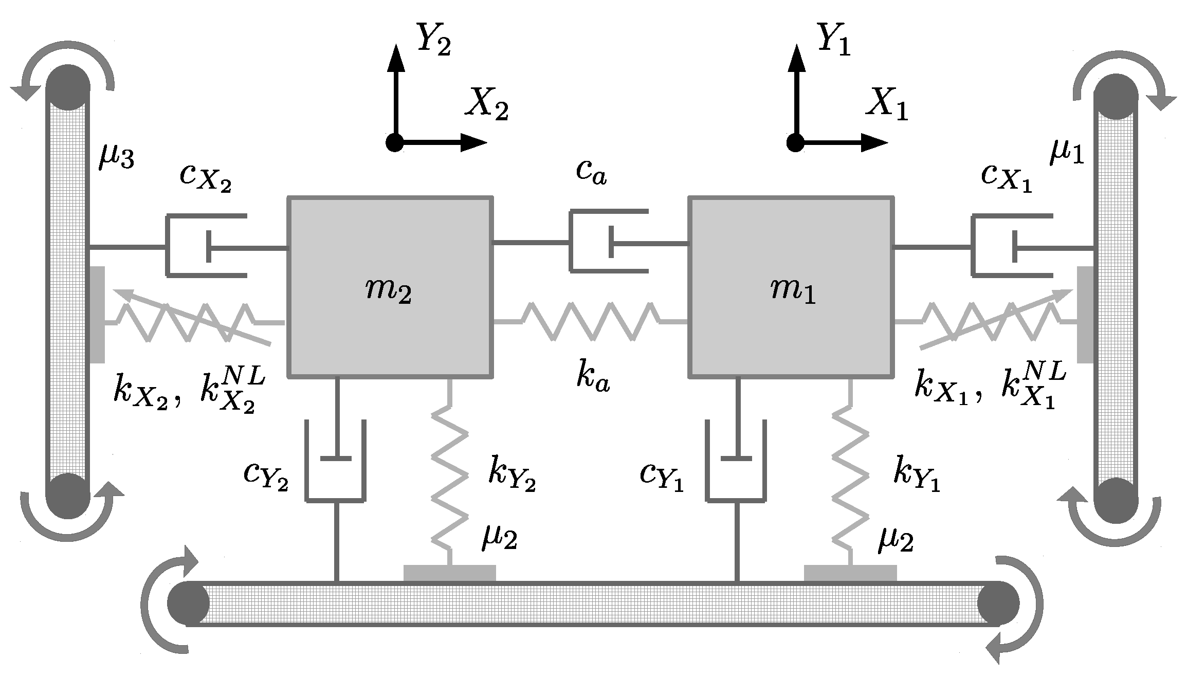
In order to analyze multi-instabilities and nonlinear friction-induced vibrations, a phenomenological lumped self-excited model was originally proposed by Dakel and Sinou [16] and then used to test new numerical strategies to predict brake squeal by Denimal et al. [17,18]. This four-degrees-of-freedom model (see Figure 1) corresponds to an extension of the two-degrees-of-freedom model proposed by Hulten [19,20]. As a reminder, this model is classically used to analyze the problems of self-exciting mechanism with constant friction related to drum brake squeal instabilities. The proposed model consists of two masses $m_1$ and $m_2$ connected to moving belts by means of four dampers and four plates supported by four different elastic springs (whose two have a cubic nonlinearity). For the sake of simplicity, the following assumptions are adopted in the present study:

• The bands and the masses are supposed to be permanently in contact because of a preload applied to the system;
• The friction forces are determined with a classical Coulomb’s law and the friction coefficient at the different contacts is supposed to be constant and equal to $\mu$. The tangential friction forces $F_t$ are related to the normal forces $F_n$ by the following formula: $F_t=\mu F_n$;
• The stick-slip phenomenon is not taken into consideration;
• The belt runs at a constant speed and the relative velocity between the bands and the masses are positive so that the tangential friction forces $F_t$ do not change.

Thus, the dynamic equation of the system is:

$$\mathbf{M}\ddot{\mathbf{X}}+\mathbf{C}\dot{\mathbf{X}}+\left(\mathbf{K}+{\mathbf{K}}_{\mu }\right)\mathbf{X}={\mathbf{F}}_{\mathbf{nl}}\left(\mathbf{X}\right)$$

(1)

where $\mathbf{X}={\left[X_1{Y}_1{X}_2{Y}_2\right]}^{\mathrm{T}}$ defines the vector of the four degrees-of-freedom of the mechanical system under study. $\mathbf{M}$, $\mathbf{C}$ and $\mathbf{K}$ correspond to the mass, damping and stiffness matrices given by:

$$\begin{array}{c}\hfill \mathbf{M}=\left[\begin{array}{cccc}{m}_1& 0& 0& 0\\ 0& m_1& 0& 0\\ 0& 0& m_2& 0\\ 0& 0& 0& m_2\end{array}\right]\end{array}$$

(2)

$$\begin{array}{c}\hfill \mathbf{C}=\left[\begin{array}{cccc}{c}_{X_1}+c_a& 0& -c_a& 0\\ 0& c_{Y_1}& 0& 0\\ -c_a& 0& c_{X_2}+c_a& 0\\ 0& 0& 0& c_{Y_2}\end{array}\right]\end{array}$$

(3)

$$\begin{array}{c}\hfill \mathbf{K}=\left[\begin{array}{cccc}{k}_{X_1}+k_a& 0& -k_a& 0\\ 0& k_{Y_1}& 0& 0\\ -k_a& 0& k_{X_2}+k_a& 0\\ 0& 0& 0& k_{Y_2}\end{array}\right]\end{array}$$

(4)

The vector of the nonlinear efforts ${\mathbf{F}}_{\mathbf{nl}}\left(\mathbf{X}\right)$ and the stiffness contribution ${\mathbf{K}}_{\mu }$ due to friction are defined as follows:

$$\begin{array}{c}\hfill {\mathbf{K}}_{\mu }=\left[\begin{array}{cccc}0& {\mu }_2{k}_{Y_1}& 0& 0\\ -{\mu }_1{k}_{X_1}& 0& 0& 0\\ 0& 0& 0& {\mu }_2{k}_{Y_2}\\ 0& 0& -{\mu }_3{k}_{X_2}& 0\end{array}\right]\end{array}$$

(5)

$$\begin{array}{c}\hfill {\mathbf{F}}_{\mathbf{nl}}\left(\mathbf{X}\right)={\left[\begin{array}{cccc}-k_{X_1}^{NL}{X}_1^3& {\mu }_1{k}_{X_1}^{NL}{X}_1^3& -k_{X_2}^{NL}{X}_2^3& {\mu }_3{k}_{X_2}^{NL}{X}_2^3\end{array}\right]}^T\end{array}$$

(6)

For the rest of the study, the following sets of parameters are used [16]: $m_1=m_2=1$ kg; $c_{X_1}=c_{X_2}=c_{Y_1}=c_{Y_2}=c_a=1$ Ns/m; $k_{X_1}=6000$ N/m; $k_{X_2}=k_{Y_1}=3000$ N/m; $k_{Y_2}=1000$ N/m; $k_a=100$ N/m; $k_{X_1}^{NL}=k_{X_2}^{NL}={10}^6$ N/m${}^3$. Moreover the three coefficients of friction are assumed to be equal (i.e., ${\mu }_1={\mu }_2={\mu }_3$). The values of all of these parameters have been chosen:

• To allow realistic results for the physical quantities observed (instability frequencies, vibration amplitudes, velocities, etc.) and thus test the relevance of the control in a context close to the engineering problem in the real world;
• To validate the control for a mechanical system subjected to more or less complex nonlinear behaviors (with mono or multi-instabilities in the presence of friction).

2.2. Stability Analysis, Transient and Self-Excited Vibrations

Two main strategies exist to predict squeal. The first one corresponds to the well-known Complex Eigenvalue Analysis (CEA) which is to determine the stability of the equilibrium point of the system. Even if this first step is essential to estimate the propensity of instability events in a design process, the stability analysis is often over- or under-predictive [21] due to the fact that all instabilities predicted by the CEA do not necessarily participate in the nonlinear self-sustaining dynamic response and moreover some frequencies of the dynamic response might not be identified by the CEA. This is the reason why a prediction of the vibratory regime and a self-sustained vibration analysis are generally performed as a second step.

The prediction of instabilities is based on the CEA of the system linearized at the static sliding equilibrium point ${\mathbf{X}}_0$. This equilibrium point is determined by solving the nonlinear static equation

$$\left(\mathbf{K}+{\mathbf{K}}_{\mu }\right){\mathbf{X}}_0={\mathbf{F}}_{\mathbf{nl}}\left({\mathbf{X}}_0\right)$$

(7)

Therefore the eigenvalue analysis of the characteristic linearized equation at the equilibrium point ${\mathbf{X}}_0$ can be rewritten as follows:

$$\det \left({\lambda }^2\mathbf{M}+\lambda \mathbf{C}+\mathbf{K}+{\mathbf{K}}_{\mu }-{\mathbf{J}}_{\mathbf{nl}}\left({\mathbf{X}}_0\right)\right)=0$$

(8)

where ${\mathbf{J}}_{\mathbf{nl}}\left({\mathbf{X}}_0\right)$ corresponds to the Jacobian matrix of nonlinear efforts ${\mathbf{F}}_{\mathbf{nl}}$ at the equilibrium point. $\lambda$ define the complex eigenvalues of the system. If all eigenvalues have negative real parts, the system is stable. If at least one eigenvalue has positive real part, the system is unstable. The imaginary part of the associated positive eigenvalue defines the pulsation of the associated unstable mode.

Figure 2 displays the evolution of real parts and frequencies as a function of the friction coefficient $\mu$ and the associated stability analysis of the mechanical system in the complex plan. The curves highlight the classical mode coupling: as the friction coefficient increases, the imaginary parts increase or decrease slowly. For $\mu =0.34$, the first Hopf bifurcation point occurs with the appearance of a coalescence pattern (i.e., coupling between two stable and unstable modes around 10 Hz). For $0.34<\mu <0.48$, the system has one instability (i.e., one mode with a positive real part). For $\mu >0.48$, a new Hopf bifurcation point occurs with the appearance of a second coalescence pattern around 6.6 Hz and the mechanical system has two instabilities. It can be noted that after each Hopf bifurcation point the frequencies of the two modes remain close and their associated real parts become opposite. For the reader comprehension, the evolution of the real part and frequency of each eigenvalue in regard to the friction coefficient is defined by a specific color: blue for the 1st mode; yellow for the 2nd mode; orange for the 3rd mode; and purple for the 4th mode.

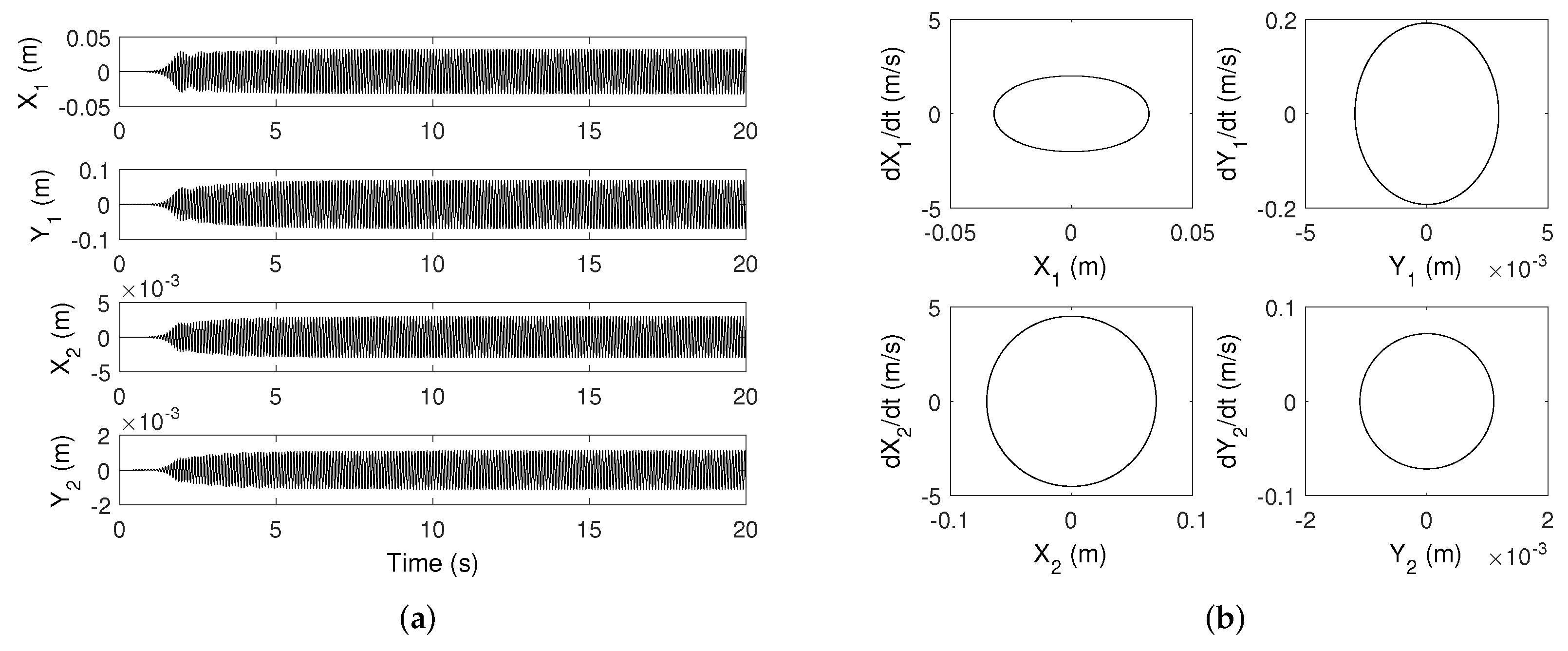
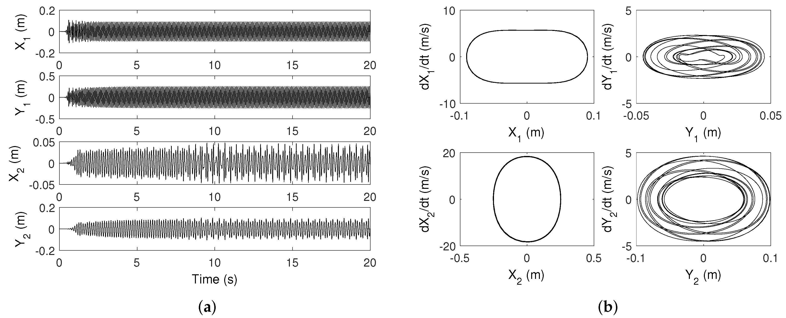
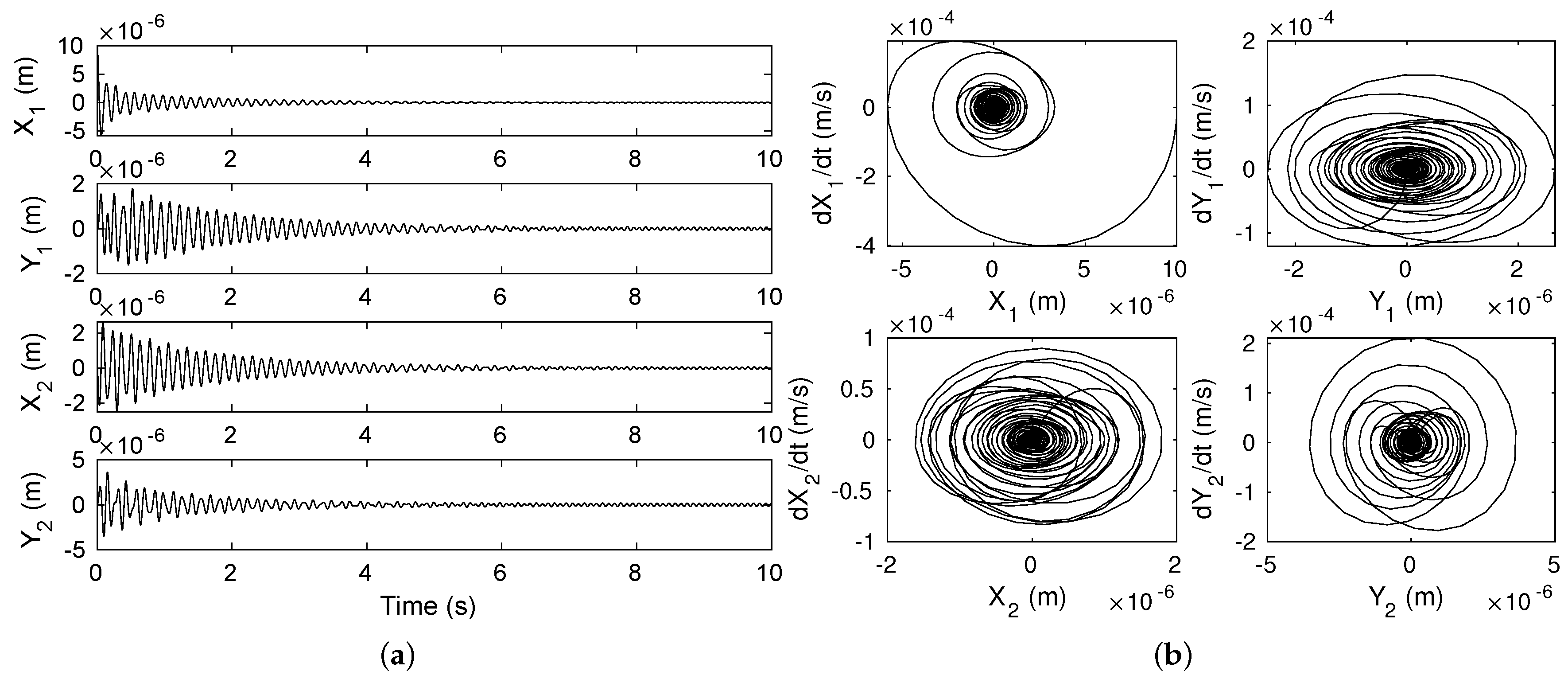
Due to the appearance of an unstable equilibrium point, nonlinear transient and steady-state self-excited friction-induced vibrations can be generated. For the sake of brevity, only the two cases that will be considered throughout the paper are shown and discussed. Figure 3 and Figure 4 illustrate two classical transient and self-excited vibrations for different friction coefficients (i.e., $\mu =0.4$ and $\mu =0.7$, respectively) and the associated limit cycles amplitudes. It can be observed that for some cases a fast increase of the transient oscillations (i.e., the initial growing transient oscillations with the highest amplitudes) is followed by a slight decrease until the nonlinear periodic motions (see for example Figure 4 for $X_1$). Moreover a complex nonlinear behavior with quasi-periodic motion is observed for $\mu =0.7$ (see for example the limit cycles $\left(Y_1,\dot{Y_1}\right)$ and $\left(Y_2,\dot{Y_2}\right)$ on Figure 4).

For the rest of the study, these two cases will serve as reference cases in order to investigate the relevance and performance of a controller for the self-excited nonlinear system subjected to friction-induced vibration in the presence of one or two unstable modes.

3. Active Control Design

3.1. Active Feedback Linearization

The aim of feedback linearization is to make a nonlinear system linear using active control. The principle is to define a control vector which allows to completely neutralize the nonlinear phenomena. The feedback linearization method using the Lie algebra [8,9] can be simplified when the system dynamics is defined by second-order differential equations as explained by Jiffri et al. [11]. The dynamic equation of the system studied is defined including the controller by

$$\begin{array}{c}\hfill \mathbf{M}\ddot{\mathbf{X}}+\mathbf{C}\dot{\mathbf{X}}+(\mathbf{K}+{\mathbf{K}}_{\mu })\mathbf{X}={\mathbf{F}}_{\mathbf{nl}}\left(\mathbf{X}\right)+{\mathbf{B}}_u\mathbf{u}\end{array}$$

(9)

where $\mathbf{u}$ and ${\mathbf{B}}_u$ are the control vector and the matrix of the distribution of the control on the different degrees-of-freedom respectively. In the case of complete Input-Output linearization using n input, n output and n degrees-of-freedom, the matrix ${\mathbf{B}}_u$ is square and the control vector u applied to the nonlinear system can be chosen so that

$$\begin{array}{c}\hfill \mathbf{u}={\mathbf{B}}_u^{-1}\left(\overline{\mathbf{u}}-{\mathbf{F}}_{\mathbf{nl}}\left(\mathbf{X}\right)\right)\end{array}$$

(10)

where $\overline{\mathbf{u}}$ is the artificial command applied to the linear system. Equation (9) can then be written using Equation (10) in a linear form

$$\begin{array}{c}\hfill \mathbf{M}\ddot{\mathbf{X}}+\mathbf{C}\dot{\mathbf{X}}+(\mathbf{K}+{\mathbf{K}}_{\mu })\mathbf{X}=\overline{\mathbf{u}}\end{array}$$

(11)

Therefore, from the knowledge of the nonlinearities, this choice of control vector cancels fully the nonlinear force.

3.2. Linear Poles Placement

Pole placement can then be done using the state space form of Equation (11) with $\mathbf{Y}={\left[\begin{array}{cc}\mathbf{X}& \dot{\mathbf{X}}\end{array}\right]}^{\mathbf{T}}$

$$\begin{array}{c}\hfill \left\{\begin{array}{c}\dot{\mathbf{Y}}=\mathbf{A}\mathbf{Y}+\mathbf{B}\overline{\mathbf{u}}\hfill \\ \overline{\mathbf{u}}=-\mathbf{G}\mathbf{Y}\hfill \end{array}\right.\end{array}$$

(12)

where the matrix of the system dynamics $\mathbf{A}$ and the matrix of the distribution of the control on the different degrees-of-freedom $\mathbf{B}$ are given by

$$\begin{array}{c}\hfill \mathbf{A}=\left[\begin{array}{cc}{\mathbf{0}}_{n,n}& {\mathbf{Id}}_{n,n}\\ -{\mathbf{M}}^{-\mathbf{1}}\left(\mathbf{K}+{\mathbf{K}}_{\mu }\right)& -{\mathbf{M}}^{-\mathbf{1}}\mathbf{C}\end{array}\right]\end{array}$$

(13)

and

$$\begin{array}{c}\hfill \mathbf{B}=\left[\begin{array}{c}{\mathbf{0}}_{n,n}\\ {\mathbf{M}}^{-\mathbf{1}}\end{array}\right]\end{array}$$

(14)

where ${\mathbf{Id}}_{n,n}$ denotes the $n\times n$ identity matrix. The $2n$ conjugate poles $\lambda$ of the matrix $\mathbf{A}$ can be used to compute the control gain matrix $\mathbf{G}$ using a classical pole placement algorithm [22] so that

$$\begin{array}{c}\hfill {\lambda }_c=\gamma \Re \left(\lambda \right)+j\Im \left(\lambda \right)\end{array}$$

(15)

where $j=\sqrt{-1}$. $\Re \left(\right)$ and $\Im \left(\right)$ are the real and the imaginary part respectively. ${\lambda }_c$ are the poles of the controlled system and $\gamma$ the control gain applied on the real part of the uncontrolled poles.

3.3. Numerical Simulations

With the aim of analyzing the effects of the control on the nonlinear system, a first analysis is carried out for two values of $\mu$ to show the impact of the linear and nonlinear contributions of the control vector in the dynamics of the closed-loop system. Based on the previous results without control presented in Section 2.2, the two specific following cases are chosen:

• Case 1 for $\mu =0.4$ with only one unstable mode detected by CEA and the generation of self-sustaining periodic vibrational responses;
• Case 2 for $\mu =0.7$ with two unstable modes detected by CEA and a self-sustaining quasi-periodic motion.

The impact of the choices of control gain is then studied using four different values of control gain $\gamma$. Finally, the robustness and the limits of the controller depending on the noise-to-signal ratio is examined using four levels of signal-to-noise ratio to study the impact of measurement noise or poor boundary conditions on the dynamics of the controlled system.

3.3.1. Contributions of Linear and Nonlinear Parts in the Control Vector for Different Values of $\mu$

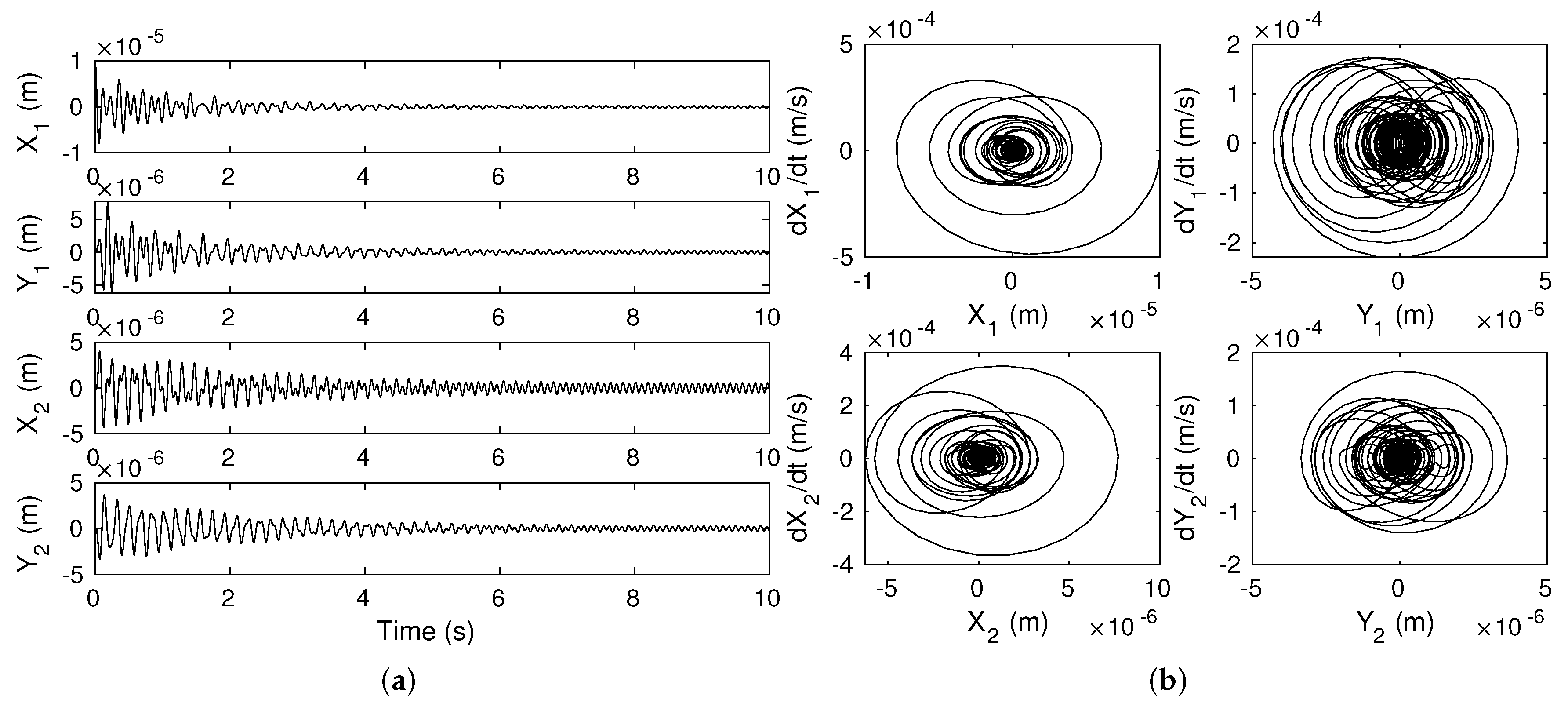
The nonlinear responses and the associated limit cycles of the system with nonlinear control with $\gamma =-0.1$ are presented in Figure 5a,b for $\mu =0.4$ (i.e., the case with only one unstable pole) and in Figure 6a,b for $\mu =0.7$ (i.e., the case with two unstable poles). In this first numerical study, $\gamma$ is just chosen to stabilize unstable poles without adding further damping. In the two cases, the control allows to stabilize the unstable poles (see Figure 5b and Figure 6b) and to decrease the level of the four degrees-of-freedom. Thus, the effectiveness of a controller to drastically reduce periodic or quasi-periodic self-sustained vibrations is demonstrated without any ambiguity. For the two cases proposed in this study, it clearly appears that the regime of rise in divergence of the oscillations does not have time to set up: the controller allows to stay with self-excited vibrations of very low level.

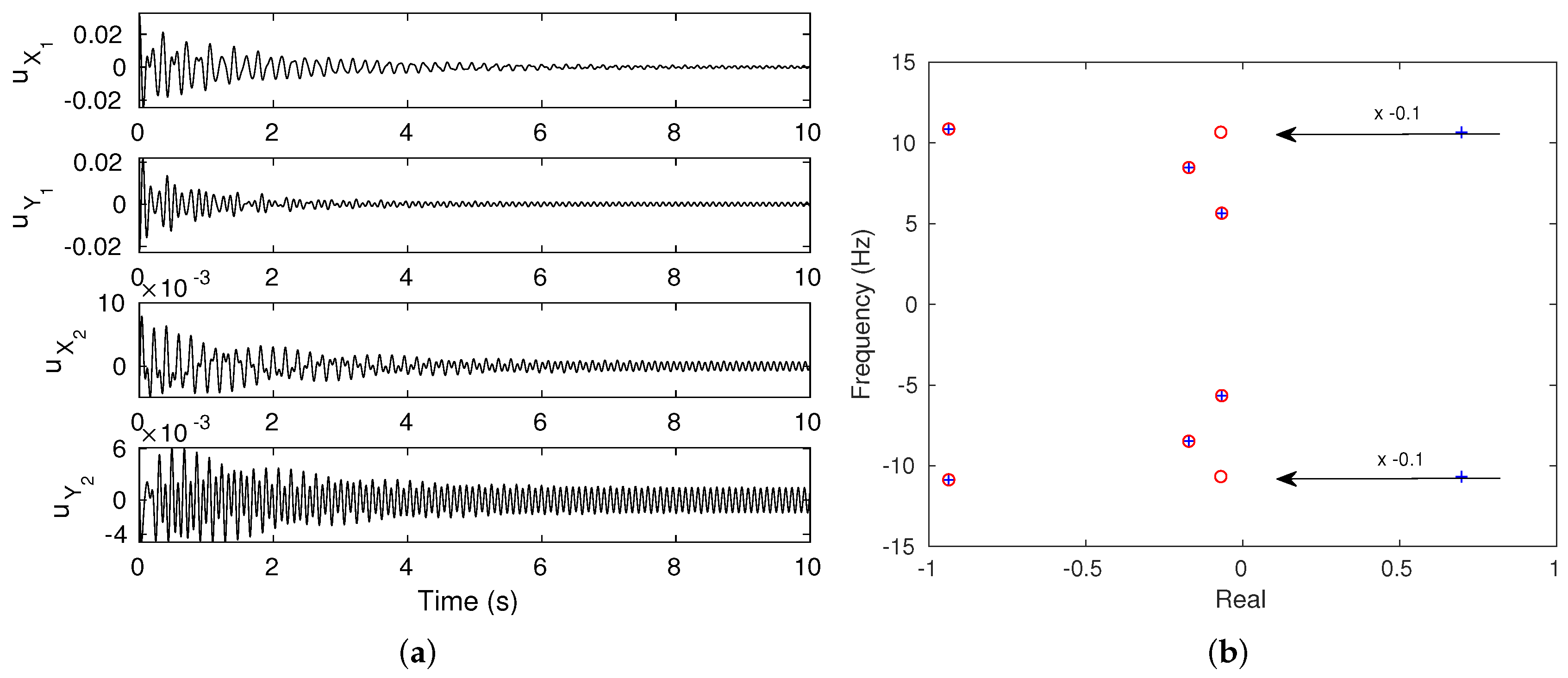
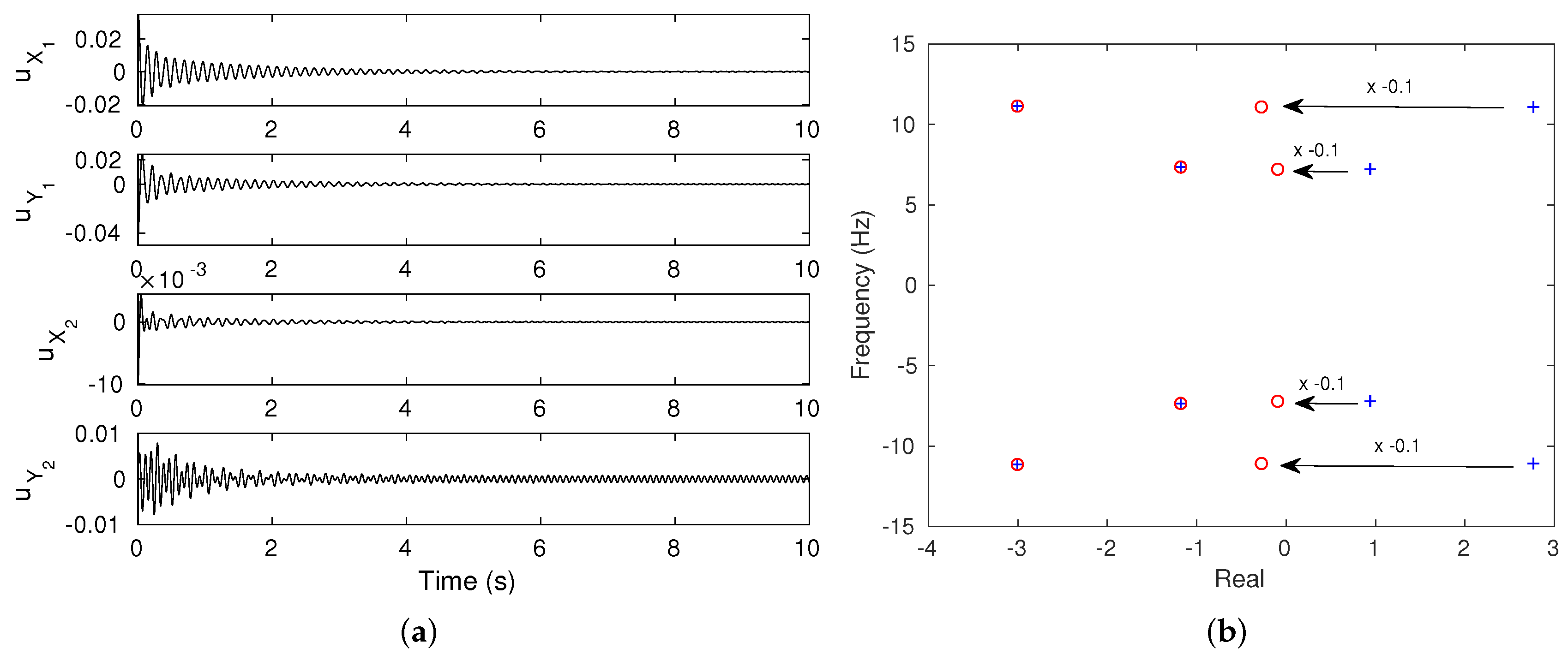
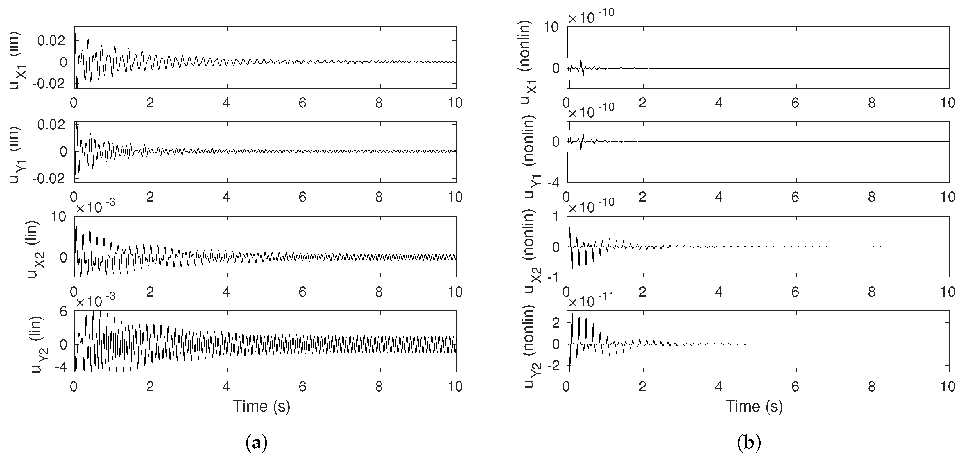
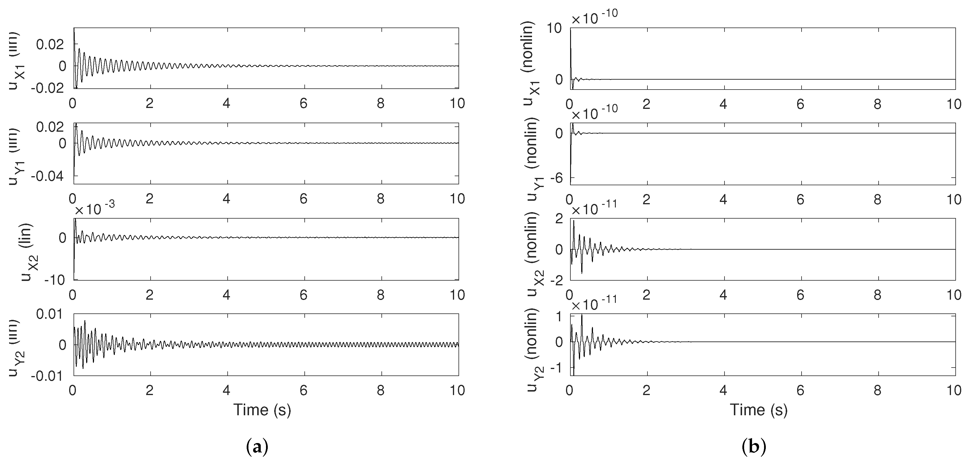
The control vector applied on $X_1$, $Y_1$, $X_2$ and $Y_2$ and the associated poles chart are presented in Figure 7a,b for $\mu =0.4$ and in Figure 8a,b for $\mu =0.7$. The linear and nonlinear contributions of the control vector are presented in Figure 9a,b for $\mu =0.4$ and in Figure 10a,b for $\mu =0.7$. As a reminder, the linear part of the control vector can be written

$$\begin{array}{c}\hfill {\mathbf{u}}_{lin}={\mathbf{B}}_u^{-1}\overline{\mathbf{u}}\end{array}$$

(16)

and the nonlinear part can be written

$$\begin{array}{c}\hfill {\mathbf{u}}_{nonlin}=-{\mathbf{B}}_u^{-1}{\mathbf{F}}_{\mathbf{nl}}\left(\mathbf{X}\right)\end{array}$$

(17)

These results show that the contribution of the nonlinear part of the control vector is negligible with respect to the linear part. This observation can be explained by the decrease of the amplitude of the system response when unstable poles are stabilized making the nonlinear force negligible. Moreover, as the control is started at t = 0 s, nonlinear phenomena do not have the time to affect drastically the response of the system and the controller is designed close to the the equilibrium point. Consequently, a simple linear control may be successfully applied on the nonlinear system. It is sufficient and as effective as a nonlinear control to reduce vibration amplitudes due to friction-induced vibration. In addition it will have the advantage from a practical point of view of being more easily implemented for an engineering problem in order to mitigate friction-induced vibration and noise such as squeal.

3.3.2. Influence of the Control Gain and Sensitivity of the Controller to the Signal-To-Noise Ratio (SNR)

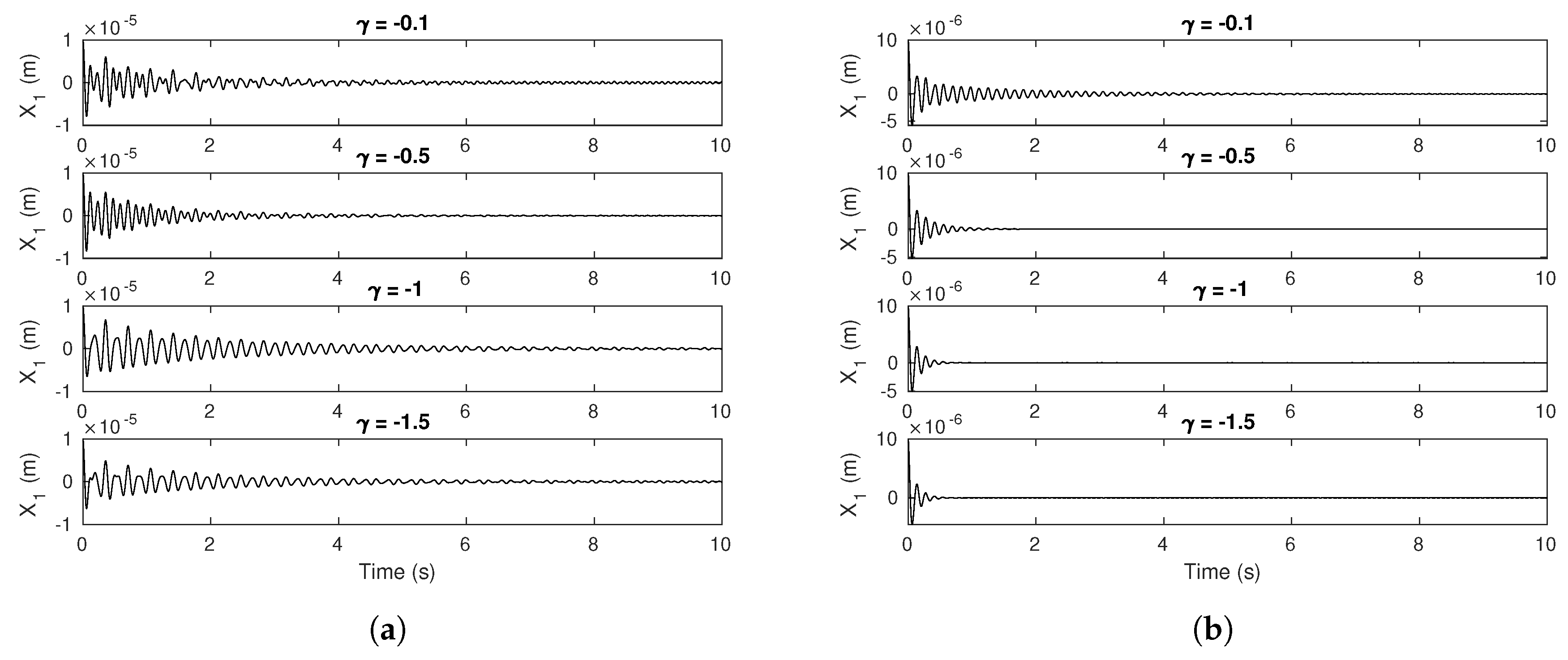
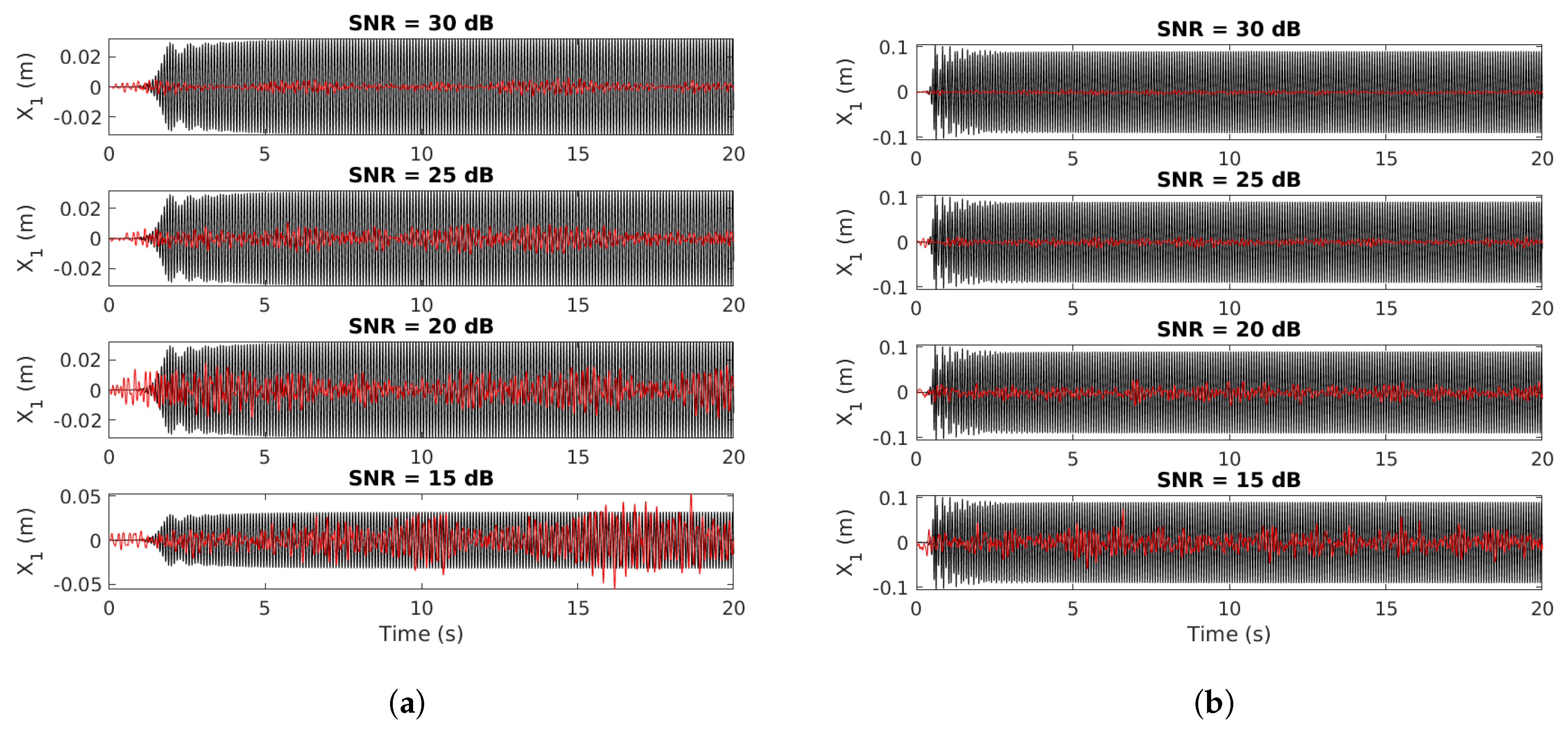
The influence of the control gain $\gamma$ on the response $X_1$ is presented in Figure 11a for $\mu =0.4$ and in Figure 11b for $\mu =0.7$. These results show that the behavior of the system is not the same in the two configurations when $\gamma$ increases from −0.1 to 1.5. For $\mu =0.7$, the increase of $\gamma$ induces a more faster damping. But for $\mu =0.4$, the increase of $\gamma$ seems to change the dynamics of the controlled system probably due to couplings between the different modes. The sensitivity of the controller to different SNR, from 30 dB to 15 dB, between the response $X_1$ and the signal used by the controller is presented in Figure 12a for $\mu =0.4$ and in Figure 12b for $\mu =0.7$. The control remains effective in the two cases up to a minimum value equal to −15 dB but with a severe loss of efficiency. For a lower value of SNR, the control can become fully inefficient and the controlled system can differ. Moreover, the decease of performances is more pronounced for $\mu =0.4$.

4. Conclusions

The possibility of using passive or active control for reducing self-excited vibrations of a mechanical system subjected to friction-induced vibration is nowadays a crucial point. In the present study, an active control design is tested to determine whether it is possible to reduce drastically nonlinear vibrations due to mono or multi-instabilities for a simplified four-degrees-of-freedom model. Some non-exhaustive interesting conclusions can be addressed:

• The use of active control makes it possible to significantly reduce periodic or quasi-periodic self-sustained vibrations (i.e., in the case of mechanical systems subjected to one or more unstable modes);
• The control gain $\gamma$ has a significant influence on system control performances. This is particularly important in a practical case where the gain has to remain on physically feasible nominal values in terms of design particularly for the amplification and the actuation part;
• The robustness of the control to the signal-to-noise ratio is proven. For the proposed study, the control remains effective up to a minimum value equal to 15 dB;
• Using nonlinear active control seems useless in the present case. Effectively, due to the fact that the control is started at the beginning of the self-excited oscillations, a simple active control based on the linearized system dynamics at the equilibrium point is sufficient.

Finally some non-exhaustive interesting further studies can be considered:

• Robustness of the control in the case of other inaccuracies possible in real systems, for example time delay, time discretization;
• Extension of control efficiency to a more real industrial brake system;
• Experimental validation of the potential of an active control design based on full and partial linearization feedback;
• Active control algorithm based on the receptance method to control the system without the knowledge of mechanical properties including nonlinearities in the case of experimental validation;
• Extension of the method in the case of stick-slip vibrations.

References

- Kinkaid, N.; O’Reilly, O.; Papadopoulos, P. Automotive disc brake squeal. J. Sound Vib. 2003, 267, 105–166. [Google Scholar] [CrossRef]
- Ouyang, H.; Nack, W.; Yuan, Y.; Chen, F. Numerical analysis of automotive disc brake squeal: A review. Int. J. Veh. Noise Vib. 2005, 1, 207–231. [Google Scholar] [CrossRef]
- Crolla, D.; Lang, A. Brake noise and vibration—State of the art. Tribol. Ser. 1991, 18, 165–174. [Google Scholar]
- Papinniemi, A.; Lai, J.; Zhao, J.; Loader, L. Brake squeal: A literature review. Appl. Acoust. 2002, 63, 391–400. [Google Scholar] [CrossRef]
- Chatterjee, S. Non-linear control of friction-induced self-excited vibration. Int. J. Nonlinear Mech. 2007, 42, 459–469. [Google Scholar] [CrossRef]
- Wang, Y.F.; Wang, D.H.; Chai, T.Y. Active control of friction-induced self-excited vibration using adaptive fuzzy systems. J. Sound Vib. 2011, 330, 4201–4210. [Google Scholar] [CrossRef]
- Snoun, C.; Bergeot, B.; Berger, S. Prediction of the dynamic behavior of an uncertain friction system coupled to nonlinear energy sinks using a multi-element generalized polynomial chaos approach. Eur. J. Mech. A-Solid 2020, 80, 103917. [Google Scholar] [CrossRef] [Green Version]
- Jakubczyk, B. Feedback Linearization of Discrete-Time-Systems. Syst. Control Lett. 1987, 9, 411–416. [Google Scholar] [CrossRef]
- Charlet, B.; Levine, J.; Marino, R. Sufficient Conditions for Dynamic State Feedback Linearization. SIAM J. Control Optim. 1991, 29, 38–57. [Google Scholar] [CrossRef]
- Nechak, L. Nonlinear control of friction-induced limit cycle oscillations via feedback linearization. Mech. Syst. Signal Process. 2019, 126, 264–280. [Google Scholar] [CrossRef]
- Jiffri, S.; Paoletti, P.; Cooper, J.E.; Mottershead, J.E. Feedback Linearisation for Nonlinear Vibration Problems. Shock Vib. 2014, 2014, 1–16. [Google Scholar] [CrossRef]
- Tehrani, M.G.; Wilmshurst, L.; Elliott, S.J. Receptance method for active vibration control of a nonlinear system. J. Sound Vib. 2013, 332, 4440–4449. [Google Scholar] [CrossRef]
- Liang, Y.; Yamaura, H.; Ouyang, H. Active assignment of eigenvalues and eigen-sensitivities for robust stabilization of friction-induced vibration. Mech. Syst. Signal Process. 2017, 90, 254–267. [Google Scholar] [CrossRef]
- Hu, X. On state observers for nonlinear systems. Syst. Control Lett. 1991, 17, 465–473. [Google Scholar] [CrossRef]
- Nechak, L. Nonlinear state observer for estimating and controlling of friction-induced vibrations. Mech. Syst. Signal Process. 2020, 139, 106588. [Google Scholar] [CrossRef]
- Dakel, M.; Sinou, J.J. Stability and nonlinear self-excited friction-induced vibrations for a minimal model subjected to multiple coalescence patterns. J. Vibroeng. 2017, 19, 604–628. [Google Scholar] [CrossRef]
- Denimal, E.; Nechak, L.; Sinou, J.J.; Nacivet, S. Kriging surrogate models for predicting the complex eigenvalues of mechanical systems subjected to friction-induced vibration. Shock Vib. 2016, 2016, 1–22. [Google Scholar] [CrossRef] [Green Version]
- Denimal, E.; Nechak, L.; Sinou, J.J.; Nacivet, S. A novel hybrid surrogate model and its application on a mechanical system subjected to friction-induced vibration. J. Sound Vib. 2018, 434, 456–474. [Google Scholar] [CrossRef]
- Hulten, J. Brake Squeal-A Self-Exciting Mechanism with Constant Friction; Technical Report, SAE Technical Paper; SAE: Warrendale, PA, USA, 1993. [Google Scholar]
- Hulten, J. Friction phenomena related to drum brake squeal instabilities. In Proceedings of the ASME Design Engineering Technical Conferences, 16th Biennial Conference on Mechanical Vibration and Noise, Sacramento, CA, USA, 14–17 September 1997. [Google Scholar]
- Sinou, J.J. Transient non-linear dynamic analysis of automotive disc brake squeal–on the need to consider both stability and non-linear analysis. Mech. Res. Commun. 2010, 37, 96–105. [Google Scholar] [CrossRef] [Green Version]
- Valášek, M.; Olgac, N. Efficient eigenvalue assignments for general linear MIMO systems. Automatica 1995, 31, 1605–1617. [Google Scholar] [CrossRef]