Efficient Deep Learning for Gradient-Enhanced Stress Dependent Damage Model

Abstract

This manuscript introduces a computational approach to micro-damage problems using deep learning for the prediction of loading deflection curves. The location of applied forces, dimensions of the specimen and material parameters are used as inputs of the process. The micro-damage is modelled with a gradient-enhanced damage model which ensures the well-posedness of the boundary value and yields mesh-independent results in computational methods such as FEM. We employ the Adam optimizer and Rectified linear unit activation function for training processes and research into the deep neural network architecture. The performance of our approach is demonstrated through some numerical examples including the three-point bending specimen, shear bending on L-shaped specimen and different failure mechanisms.

1. Introduction

Neural networks (NN) have been used for numerous applications in different areas including computational mechanics. Initially, single-layer or shallow neural networks (SNN) consisted only of one input and one output layer. Later on, additional hidden layers were added to the network architecture resulting in so-called deep neural networks (DNN).

Table 1. The branches of the neural network depending on the layer architecture.

Single-Layer Neural Networks		Input Layer-Output Layer
	Shallow	Input Layer-Hidden Layer
Multilayer-Layer	Neural Networks	-Output Layer
Neural Networks	Deep	Input Layer-Hidden Layers
	Neural Networks	-Output Layers

gives a brief summary of different network architectures. Neural networks or more specifically deep neural networks suffer from three major difficulties, i.e., (a) vanishing gradients, (b) over-fitting and (c) computational loading. However, significant advances such as deep belief networks (DBN) [1], rectified linear unit (ReLU) activation functions [2], drop-out algorithms [3] or back-propagation algorithms and associated tools have contributed to the popularity of DNN. The vanishing gradient problem for instance has been significantly alleviated thanks to the RELU activation function and cross entropy-driven learning techniques. Nonetheless, certain issues such as over-fitting still remains a challenge in deep neural networks. Common techniques to address such problems include regularization techniques.

We recall that the crucial idea behind Artificial Neural Network (ANN) is that many neurons can be joined together by connecting weights to conduct complex computations. The structure is often demonstrated as a graph or a map whose nodes are the neurons and each (directed) edge in the graph connects the output to the input of the associated neurons. Deep learning methods, representative of learning methods with multiple processing layers in the hidden layers, consist of linear and non-linear transformations [4,5]. Some simplifications of the problems stem from their need for a usually very strong CPU and a noticeably long time to detect and analyse slow convergence behaviour. For complex problems, the solution could be non-existent. A newer method or a faster algorithm has yet to be found in recent decades.

While machine learning (ML) approaches have been extensively and successfully used in numerous areas, its application in “modeling and simulation” is still in its infancy. For instance, in medicine, ML has been employed in diagnostics where it outperforms the diagnosis of established physicians [6]. The authors of [7] have applied successfully deep learning to cellular imaging. Park et al. [8] focused on the problems of cellular imaging in regulatory genomics. Goh et al. [9] took advantage of deep learning in computational chemistry. Deep learning techniques were also applied in applications such as bio-informatics, or the public health sector [10]. On the other hand, most approaches in engineering, or more specifically computational mechanics, have been used in data-driven contexts though there are numerous other applications such as the direct solution of partial differential equations [11], which have the potential to drastically accelerate the design to analysis time and the way modeling and simulation is performed. In the data-driven context, neural networks have commonly been used in the context of constitutive models [12,13] as an alternative to traditional constitutive models. The models in [14,15,16] presented interesting approaches to capture the response of anisotropic materials. New training algorithms for specific constitutive laws have been presented in [17,18]. However, setting up the network architecture for such engineering problems still remains a major challenge and is often determined by trial and error. The authors of [19] exploited Deep Learning to optimize the fine-scale structure of composites. Multi-fields problems were tackled for instance in [20,21]. Recently, Lee et al. [22] has applied deep learning algorithms to structural analysis. In this manuscript, we present a novel methodology to predict the load-deflection curve by deep learning. Passing through the three-point bending as an illustrative example, we suggest some possible architectures of the deep neural networks based on the Adam optimizer. Such findings can open a new branch of research that may prove beneficial to the fourth industrial revolution, where deep learning algorithms play a major role in big data analysis of structural engineering.

2. Continuum Damage Theory

2.1. Constitutive Equations of Isotropic Damage Models

Let us assume small strain theory in the context of a scalar/isotropic damage model. The relation between the Cauchy stress tensor $\mathit{\sigma }$ and the linear strain tensor $\mathit{\epsilon }$ is given by

$$\mathit{\sigma }=(1-\omega )\mathbb{C}:\mathit{\epsilon }={\mathbb{C}}^{eff}:\mathit{\epsilon }$$

(1)

where $\omega$ denotes a monotonically increasing scalar damage variable, $\mathbb{C}$ the fourth-order elasticity tensor and ${\mathbb{C}}^{eff}=(1-\omega )\mathbb{C}$ refers to the so-called ’effective’ elasticity tensor. A value of $\omega =1$ indicate a completely damaged material while the material is intact for a value o $\omega =0$. The evolution of the damage variable is commonly governed by a scalar state variable $\kappa$, i.e., $\omega =\omega \left(\kappa \right)$. The Kuhn–Tucker conditions, which finally lead to a convex optimization problem, ensures that the product of the loading function f and the rate of the state variable is equal to zero:

$$\left\{\begin{array}{cc}f\hfill & \le 0\hfill \\ \dot{\kappa }\hfill & \ge 0\hfill \\ f\dot{\kappa }\hfill & =0\hfill \end{array}\right.$$

(2)

${\epsilon }_{eq}$ indicating the effective strain, which is a projection of a multi-axial strain state onto a single scalar value. We consider a strain-based formulation, where the loading function is expressed in terms of the effective strain (instead of effective stresses), which facilitates the implementation in the context of displacement based finite element analysis:

$$f=f({ϵ}_{eq},\kappa )={ϵ}_{eq}-\kappa =0$$

(3)

We test two different approaches to compute ${\epsilon }_{eq}$. The first one has been presented by Mazars [23] for quasi-brittle materials and is given by

$${\epsilon }_{eq}=\sqrt{〈\mathit{\epsilon }〉:〈\mathit{\epsilon }〉}=\sqrt{{〈{\epsilon }_1〉}^2+{〈{\epsilon }_2〉}^2}$$

(4)

where $〈·〉$ indicates a Macaulay bracket while ${\epsilon }_1$ and ${\epsilon }_2$—for two-dimensional problems—denote the principal strains. For this approach, we employ an exponential evolution law for the damage variable as suggested by Peerlings et al. [24]:

$$\omega \left(\kappa \right)=1-{\displaystyle \frac{{\kappa }_0}{\kappa }}\left[1-\alpha +\alpha e^{-\beta (\kappa -{\kappa }_0)}\right]$$

(5)

where ${\kappa }_0$ stands for an initial damage threshold while the material parameters $\alpha$ and $\beta$ needs to be determined through experiments. We also employ an expression for the equivalent strain as suggested by de Vree et al. [25] and Peerlings et al. [26]:

$${\epsilon }_{eq}={\displaystyle \frac{k-1}{2k(1-\nu )}}{I}_1+{\displaystyle \frac{1}{2k}}\sqrt{{\displaystyle \frac{{(k-1)}^2}{{(1-2\nu )}^2}}{I}_1^2+{\displaystyle \frac{12k}{{(1+\nu )}^2}}{J}_2}$$

(6)

where $I_1$ indicates the first invariant of the linear strain tensor and $J_2$ refers to the second invariant of the deviatoric part of the strain tensor.

$$\left\{\begin{array}{cc}{I}_1\hfill & ={\epsilon }_{11}+{\epsilon }_{22}+{\epsilon }_{33}\hfill \\ J_2\hfill & ={\displaystyle \frac{1}{2}}{\epsilon }_{ij}{\epsilon }_{ij}-{\displaystyle \frac{1}{6}}{I}_1^2\hfill \end{array}\right.$$

(7)

The parameter k in Equation (6) determines the ratio of the compressive and tensile strength.

2.2. Gradient-Enhanced Damage Models

It is well known that local damage models lead to ill-posed boundary value problems and associated numerical difficulties such as mesh-dependent results in computational modeling. Non-local damage models as proposed [26,27,28,29,30] restore the well-posedness of the boundary value problem by introducing an intrinsic length scale which smear the crack over a certain width. In such models, the loading function is therefore expressed in terms of non-local equivalent strain ${\overline{\epsilon }}_{eq}\left(\mathit{x}\right)$ which in turn depend on the local effective strain and a weighting function $g\left(\mathit{\xi }\right)$ governing the domain of non-locality:

$${\overline{\epsilon }}_{eq}\left(\mathit{x}\right)={{\displaystyle \frac{1}{V}}}_{}\underset{V}{\int }g\left(\mathit{\xi }\right){\epsilon }_{eq}\left(\mathit{x}+\mathit{\xi }\right)dV$$

(8)

An alternative to such strongly nonlocal models are weakly nonlocal approaches [26,28,31] which are based on Taylor series expansions to approximate the effective strain. Substituting these into the Equation (8) yields a different expression for the non-local equivalent strain. However, it is well known that such formulations require $C^1$—continuity for second-order gradient models ($C^2$—continuity for fourth-order gradient enhancements), which complicates their implementation in Lagrange polynomial based finite element analysis. Implicit formulations overcome these difficulties. Differentiating twice and neglecting higher-order gradient terms of the local equivalent strain, the implicit second-order gradient model reads:

$${\epsilon }_{eq}={\overline{\epsilon }}_{eq}-{\displaystyle \frac{1}{2}}{l}_c^2{\nabla }^2{\overline{\epsilon }}_{eq}\left(\mathit{x}\right)$$

(9)

where the parameter $l_c$ indicates the intrinsic length scale, which can be regarded either as purely numerical regularization parameter or material parameter which needs to be determined through experiments or other theoretical considerations. For concrete materials, Bažant et al. related $l_c$ to the maximum aggregate size [32]. Furthermore, the following von Neumann boundary conditions need to be satisfied [28,33]:

$$\nabla {\overline{\epsilon }}_{eq}·\mathit{n}=0$$

(10)

It can be shown that the gradient enhanced damage model, Equation (9), can be expressed in terms of the principal directions and an anisotropic weight function:

$${\epsilon }_{eq}(x_1,x_2)={\overline{\epsilon }}_{eq}(x_1,x_2)-c_1{\displaystyle \frac{{\partial }^2{\overline{\epsilon }}_{eq}(x_1,x_2)}{\partial {x_1}^2}}-c_2{\displaystyle \frac{{\partial }^2{\overline{\epsilon }}_{eq}(x_1,x_2)}{\partial {x_2}^2}}$$

(11)

where $c_1$, $c_2$ are the weighting factors. More details about the derivation of above described gradient-enhanced damage model and its implementation can be found for instance in [26].

3. Training Data

3.1. Optimizers

In machine learning (ML) approaches, the weights and biases of the network (see Figure 1) are obtained through minimizing an objective function. Commonly, gradient descent methods are employed in ML. The update of the gradient descent has the form ${\mathit{x}}_{k+1}={\mathit{x}}_k-\eta {\nabla }_{\mathit{x}}f\left({\mathit{x}}_k\right)$, $\eta$ being the step size, which is also referred to as learning rate. Gradient descent methods are based on so-called batches employed to calculate the gradient in a single iteration. Commonly, the batch is the entire data set. In addition, a batch can be enormous. A very large batch may cause even a single iteration to take a very long time in computation. By choosing examples from a data set at random, it could estimate (albeit noisily) a big average from a much smaller one. Stochastic gradient descent (SGD) takes this idea to the extreme—it uses solely one example (a batch size of 1) per iteration. Every one computation for all data points, it is called one epoch. The term “stochastic” implies that the one example comprising each batch is chosen arbitrarily. The mini-batch stochastic gradient descent method (mini-batch SGD) is a compromise between the full-batch iteration and SGD. A mini-batch is usually between 10 and 1000 examples, chosen at random. Mini-batch SGD reduces the amount of noise in SGD but is still more efficient than full-batch. It is well known that the steepest gradient descent faces difficulties in areas where surface curves exhibit different gradients in different dimensions, which frequently occurs around local optima. To reduce the risk of getting stuck in local optima, we take advantage of the Momentum Method, which shows analogies to the equations governing the movement of particles in a viscous medium:

$$\begin{array}{cc}{\mathit{x}}_{k+1}\hfill & ={\mathit{x}}_k-{\mathit{v}}_k\hfill \\ {\mathit{v}}_k\hfill & =\gamma {\mathit{v}}_{k-1}+\eta {\nabla }_{\mathit{x}}f\left({\mathit{x}}_k\right)\hfill \end{array}$$

(12)

where the parameter $\gamma \approx 0.9$ governs the updating of the iterations within the stochastic gradient descent method (SGDM). This approach is commonly employed with the back propagation algorithm, which will be explained later. However, the momentum method is based on the situation where a ball rolling downhill blindly follows the slope. A smarter ball would slow down before the slope goes up again, which is the essence of the Nesterov Accelerated Gradient (NAG) approach [34]. Therefore, the changing of momentum is computed, which is simply the sum of the momentum vector and the gradient vector at the current step. The changing of the Nesterov momentum is then the sum of the momentum vector and the gradient vector at the approximation of the next step:

$$\begin{array}{cc}{\mathit{x}}_{k+1}\hfill & ={\mathit{x}}_k-{\mathit{v}}_k\hfill \\ {\mathit{v}}_k\hfill & =\gamma {\mathit{v}}_{k-1}+\eta {\nabla }_{\mathit{x}}f\left({\mathit{x}}_k-\gamma {\mathit{v}}_{k-1}\right)\hfill \end{array}$$

(13)

Gradients of complex functions as used in DNN tend to either vanish or explode. These vanishing/exploding problems become more pronounced with increasing complexity of the function. These issues can be alleviated by an adapted learning rate method, named RMSProp, which was suggested by Geoff Hinton in Lecture 6e of his Coursera Class. The idea is based on a moving average of the squared gradients, which normalizes the gradient. This approach proves effective to balance the step size by decreasing the step for large gradient to avoid explosion while increasing the step for small gradients, which evenutally alleviates the vanishment problem:

$$\begin{array}{cc}{r}_k\hfill & =(1-\beta )·{\left[{\nabla }_{\mathit{x}}f\left({\mathit{x}}_k\right)\right]}^2+\beta r_{k-1}\hfill \\ {\mathit{v}}_{k+1}\hfill & ={\displaystyle \frac{\eta }{\sqrt{r_k}}}{\nabla }_{\mathit{x}}f\left({\mathit{x}}_k\right)\hfill \\ {\mathit{x}}_{k+1}\hfill & ={\mathit{x}}_k-{\mathit{v}}_{k+1}\hfill \end{array}$$

(14)

where the so-called squared gradient decay factor $\beta$ ranges from 0 to 1; we employ the suggested value of $\beta \approx 0.9$. Another method, that calculates learning rates adaptively for each parameter is the Adaptive Moment Estimation (Adam) [35]. Adam keeps an exponentially decaying average of past gradients ${\mathit{v}}_k$ as well. However, in contrast to the momentum method, Adam can be seen as a heavy ball with friction, that prefers flat minima in the error surface. The past decaying averages and squared gradients ${\mathit{v}}_k$ and $r_k$ can be obtained by

$$\begin{array}{cc}{\mathit{v}}_k\hfill & ={\beta }_1{\mathit{v}}_{k-1}+(1-{\beta }_1){\nabla }_{\mathit{x}}f\left({\mathit{x}}_k\right)\hfill \\ r_k\hfill & ={\beta }_2{r}_{k-1}+(1-{\beta }_2)·{\left[{\nabla }_{\mathit{x}}f\left({\mathit{x}}_k\right)\right]}^2\hfill \end{array}$$

(15)

${\mathit{v}}_k$ and $r_k$ being estimates of the first and second moment, which are the mean and the uncentered variance of the gradients, respectively. To avoid the bias towards zero vectors for the initialized vectors ${\mathit{v}}_k$ and $r_k$, we employ corrected first and second moment estimates as suggested by the authors of Adam:

$$\begin{array}{cc}{\mathit{v}}_k\hfill & ={\displaystyle \frac{{\mathit{v}}_k}{1-{\beta }_1^t}}\hfill \\ r_k\hfill & ={\displaystyle \frac{r_k}{1-{\beta }_2^t}}\hfill \end{array}$$

(16)

Subsequently, we use the Adam update rule given by

$${\mathit{x}}_{k+1}={\mathit{x}}_k-{\displaystyle \frac{\eta }{\sqrt{r_k}+ϵ}}{\mathit{v}}_k$$

(17)

3.2. Activation Functions

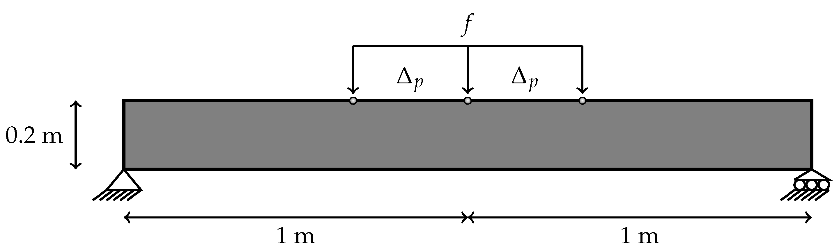
Let us consider a three-point bending beam as illustrated in Figure 2. We assume plane stress conditions and a beam thickness of $h=$$0.05$ m. The material parameters are: Young’s modulus $E=20$ (GPa), Poisson’s ratio $\nu =0.2$, softening parameters $\alpha =0.99$, $\beta =500$, ${\kappa }_0={10}^{-4}$. We employ the formulation for the equivalent strain as in Equation (4). The input of the process are locations $l_f$ where the force f is applied which will be created by 120 different positions from ${\displaystyle \frac{L}{2}}-{\mathsf{\Delta }}_p$ to ${\displaystyle \frac{L}{2}}+{\mathsf{\Delta }}_p$ where $L=2$ (m) denotes the length of the specimen and $2{\mathsf{\Delta }}_p$ indicates the span of the various forces. For each input, the vector of output is formed by ${[u_1,\cdots ,u_{31},f_1,\cdots ,f_{31}]}^T$ which $(u_i,f_i)$$\forall i=1,\cdots ,31$ are points of loading deflection curve. Therefore, the matrix of output is a $62\times 120$ matrix. The model of deep learning aims to minimize the loss between data and simulation values. The objective function is a loss function that comes from an approximate function f called activation function and the training data from simulation g:

$$loss\left(l_f\right)=∥g\left(l_f\right)-f\left(l_f\right)∥$$

(18)

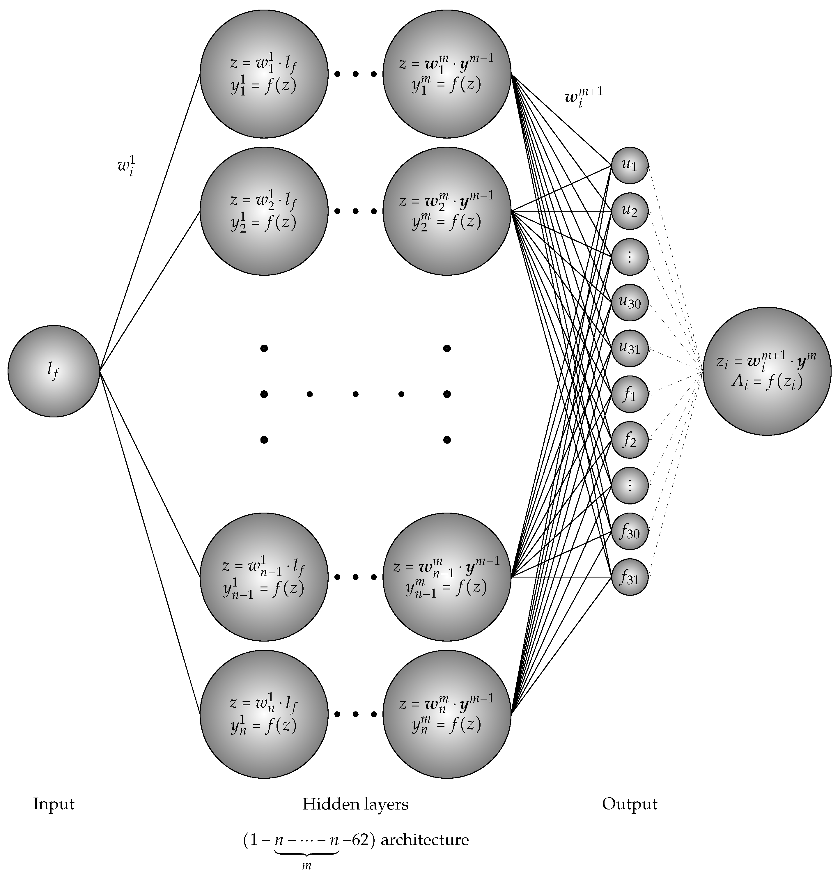
where $g:\mathbb{R}⟶{\mathbb{R}}^{62}$ which is defined by $g\left(l_f\right)=\left[\begin{array}{c}\mathit{u}\hfill \\ \mathit{f}\hfill \end{array}\right]={[u_1,\cdots ,u_{31},f_1,\cdots ,f_{31}]}^T$ based on the gradient-enhanced damage models. The roles of activation functions are are illustrated in Figure 1 and the list of different types of mostly used activation functions is shown in

Table 2. Activation functions.

Name	Equation	Derivative
Identity $(-\infty ,+\infty )$	$f\left(z\right)=z$	$f^{\prime }\left(z\right)=1$
Logistic $(0,1)$	$f\left(z\right)={\displaystyle \frac{1}{1+e^{-z}}}$	$f^{\prime }\left(z\right)=f\left(z\right)\left[1-f\left(z\right)\right]$
SoftPlus $(0,+\infty )$	$f\left(z\right)=ln(1+e^z)$	$f^{\prime }\left(z\right)={\displaystyle \frac{1}{1+e^{-z}}}$
TanH $\left(-1,1\right)$	$f\left(z\right)=Tanh\left(z\right)$	$f^{\prime }\left(z\right)=1-f{\left(z\right)}^2$
Rectified Linear Unit (ReLU) $(0,+\infty )$	$f\left(z\right)=\left\{\begin{array}{cc}0,\hfill & z<0\hfill \\ z,\hfill & z\ge 0\hfill \end{array}\right.$	$f^{\prime }\left(z\right)=\left\{\begin{array}{cc}0,\hfill & z<0\hfill \\ 1,\hfill & z\ge 0\hfill \end{array}\right.$

.

3.3. Back-Propagation Algorithm

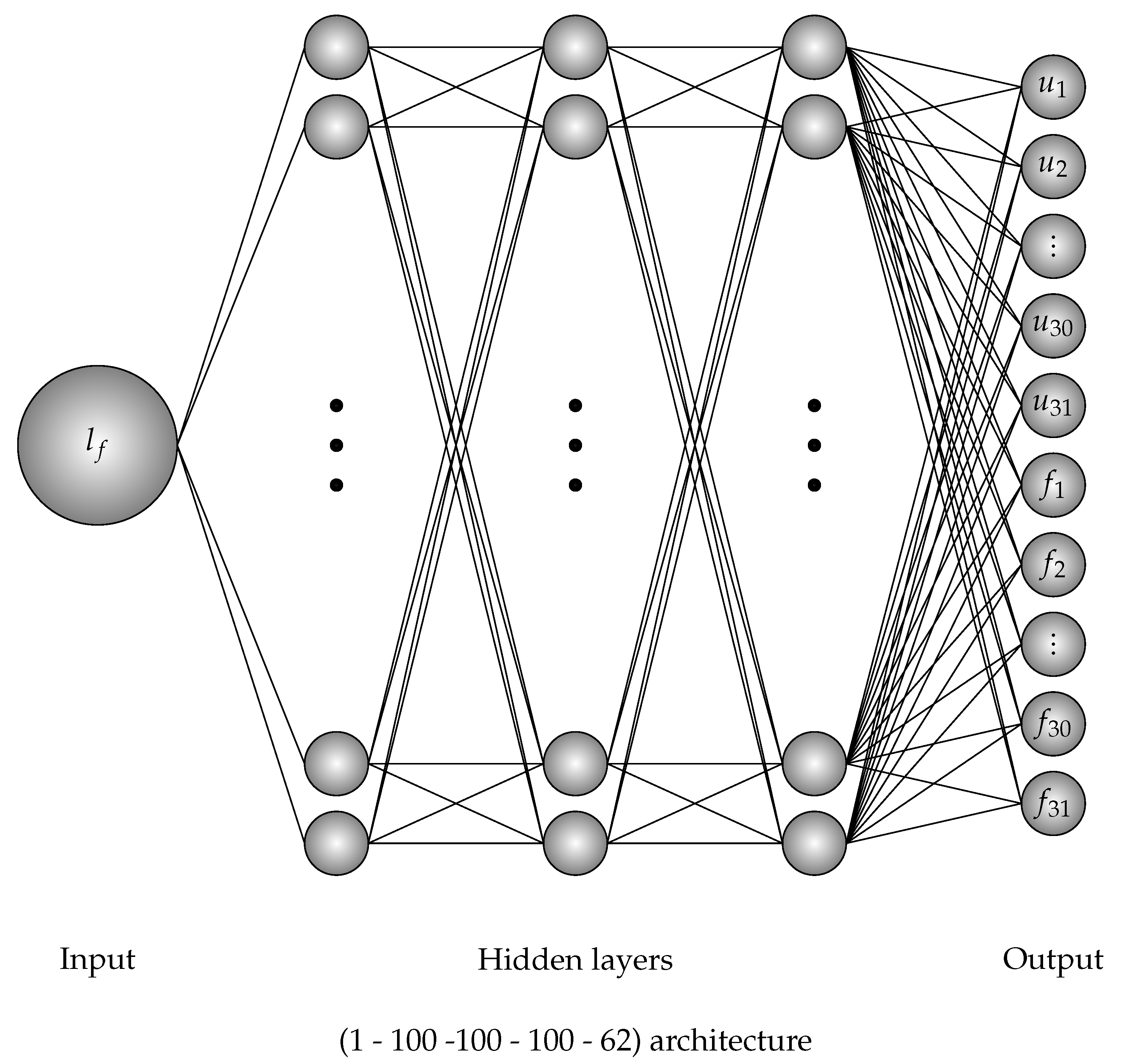
Though the back-propagation algorithm can be traced back to the 1970s, its popularity grew with the seminal paper of Rumelhart et al. [36]. It has become the ’backbone’ of many efficient machine learning tools such as Pytorch or Tensorflow. The back-propagation algorithm basically minimizes the error function in weight space by the method of gradient descent. Mathematically, the input and output are in matrix form $(\mathit{X},\mathit{Y})$ where $X\in {\mathbb{R}}^{d\times n}$ and $Y\in {\mathbb{R}}^{k\times n}$, d designate the number of input parameters, k is number of output parameters and n is number of training data. After calculating the output from the input of a mini-batch $\mathit{X}$, the activation ${\mathit{y}}^l$ at each hidden layer are saved where $l=1,\cdots ,m$ is the order of hidden layers. At the output layer, the derivative of the loss function with respect to z are calculated ${\mathit{e}}^m={\displaystyle \frac{\partial J}{\partial {\mathit{z}}^m}}$ where $J={\displaystyle \frac{1}{n}}{\sum }_{i=1}^n{∥{\overline{\mathit{y}}}_i-{\mathit{y}}_i∥}_2^2$. Hence, the gradient can be computed ${\displaystyle \frac{\partial J}{\partial {\mathit{w}}^m}}={\mathit{y}}^{m-1}{\mathit{e}}^m$. For $l=m-1,\cdots ,1$, the derivatives ${\mathit{e}}^l=\left({\mathit{w}}^{l+1}{\mathit{e}}^{l+1}\right)\otimes f^{\prime }\left({\mathit{z}}^l\right)$ are determined where the operator ⊗ means element wise product. Finally, the gradient is updated by ${\displaystyle \frac{\partial J}{\partial {\mathit{w}}^l}}={\mathit{y}}^l{\mathit{e}}^l$ which apparently requires the continuity and differentiability of the error function. Applicatively in the three-point bending specimen, the training data will be collected by the gradient-enhanced damage models and the training process based on the $(1-100-100-100-62)$ architecture in Figure 3. Because of the symmetric of the specimen, the loading deflection curve are quite similar in the left from ${\displaystyle \frac{L}{2}}-{\mathsf{\Delta }}_p$ to ${\displaystyle \frac{L}{2}}$ and in the right from ${\displaystyle \frac{L}{2}}$ to ${\displaystyle \frac{L}{2}}+{\mathsf{\Delta }}_p$ with regards to the middle point. Hence, it is a good idea to divide the data into two parts, the left part and the right part with respect to the middle point. Thus, the training is separated into two processes with 61 data for each case.

3.4. Scaled Layer

For the material problem which will be discussed in Section 5, the input data were built by different parameters. Due to the wide range of these, some data can be as large as Young’s modulus or softening parameter $\beta$ whereas other ones can be as small as the critical value of equivalent strain. This presents some limitations to the sensitive input and the training. To overcome these issues, a scaled layer based on a convex combination is introduced to reduce the overload input data and increase the tiny ones. Let s be a bijection from the range $[min,max]$ of a parameter to the interval $[0,1]$ which is defined by $s\left(x\right)={\displaystyle \frac{x-min}{l}}$ where min, max are the boundaries and l is the length of the parameter region. The role of the layer was applicable to both training and predicting process. The scale layer can be added at the input layer, the output layer or both of them.

4. Results and Testing

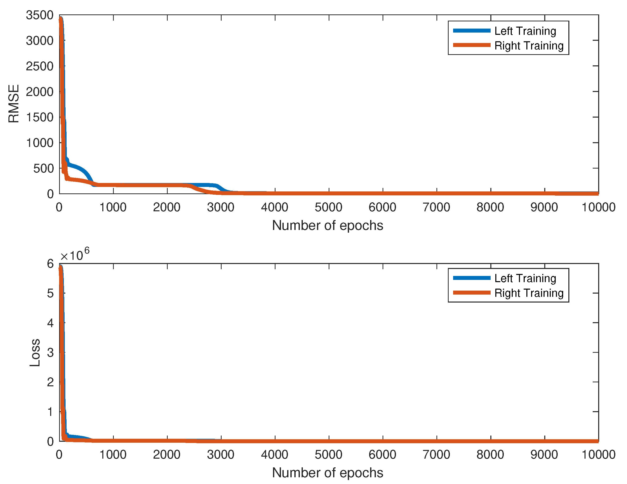
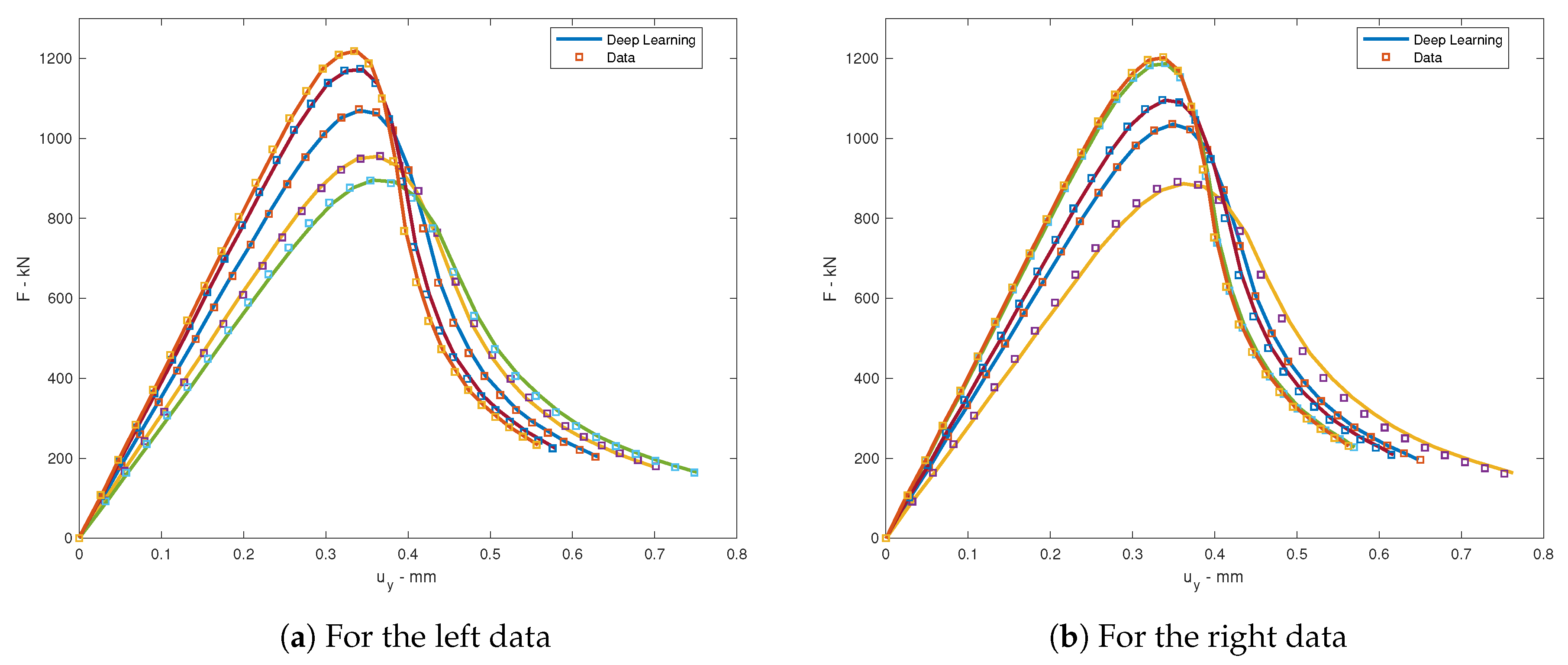
Consider back to the location force problem which was trained by Adam optimizer where Rectified Linear Unit (ReLU) activation function with back propagation algorithm was employed. The learning rate of the left data is ${\eta }_l=3\times {10}^{-3}$ and of the right data is ${\eta }_r=4\times {10}^{-3}$. For every period of a number of epochs (which is called the learning rate drop period), the learning rate is dropped base on a factor called the learning rate drop factor to let the jump steps are smaller after the period of iteration. This technique assists the convergent optimization. In this computation, the learning rate drop period is 100 epochs and the learning rate drop factor is $95\%$. The squared gradient decay factor is $0.99$. The gradient decay factor is $0.95$. The size of the mini-batch is 100 and the total of epochs is $10,000$. The training process for both left and right data are illustrated in Figure 4. The neural network architecture for this problem is $(1-100-100-100-62)$. Ten data were chosen randomly for testing. The loss values is computed by root mean square error (RMSE) and by mini-batch loss (Loss) for comparison in

Table 3. Loss values for both left and right data in the location-force problem.

Data	RMSE	Mini-Batch Loss
Left	$9.03$	$40.8$
Right	$5.03$	$12.7$

. The testing of loading deflection curves by deep learning after training and by data for both left and right is illustrated in Figure 5.

5. Numerical Examples

5.1. Dimensional Problem

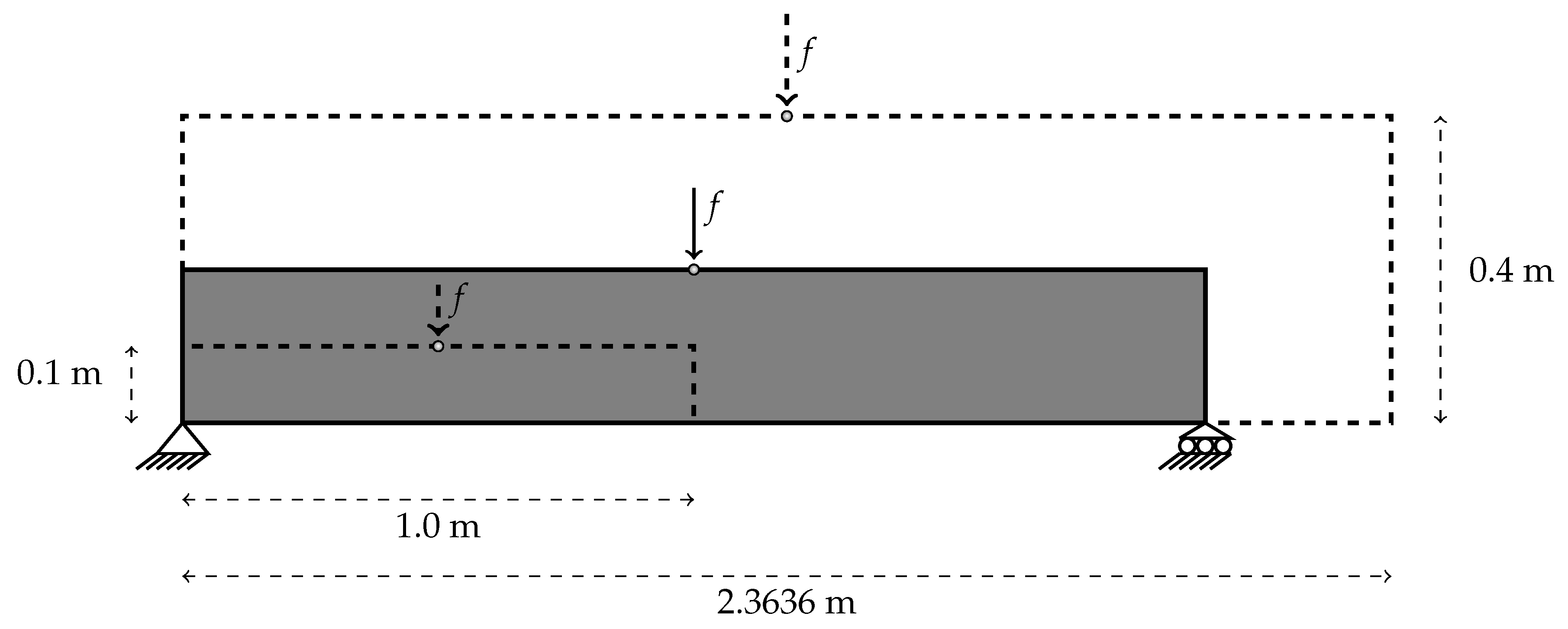
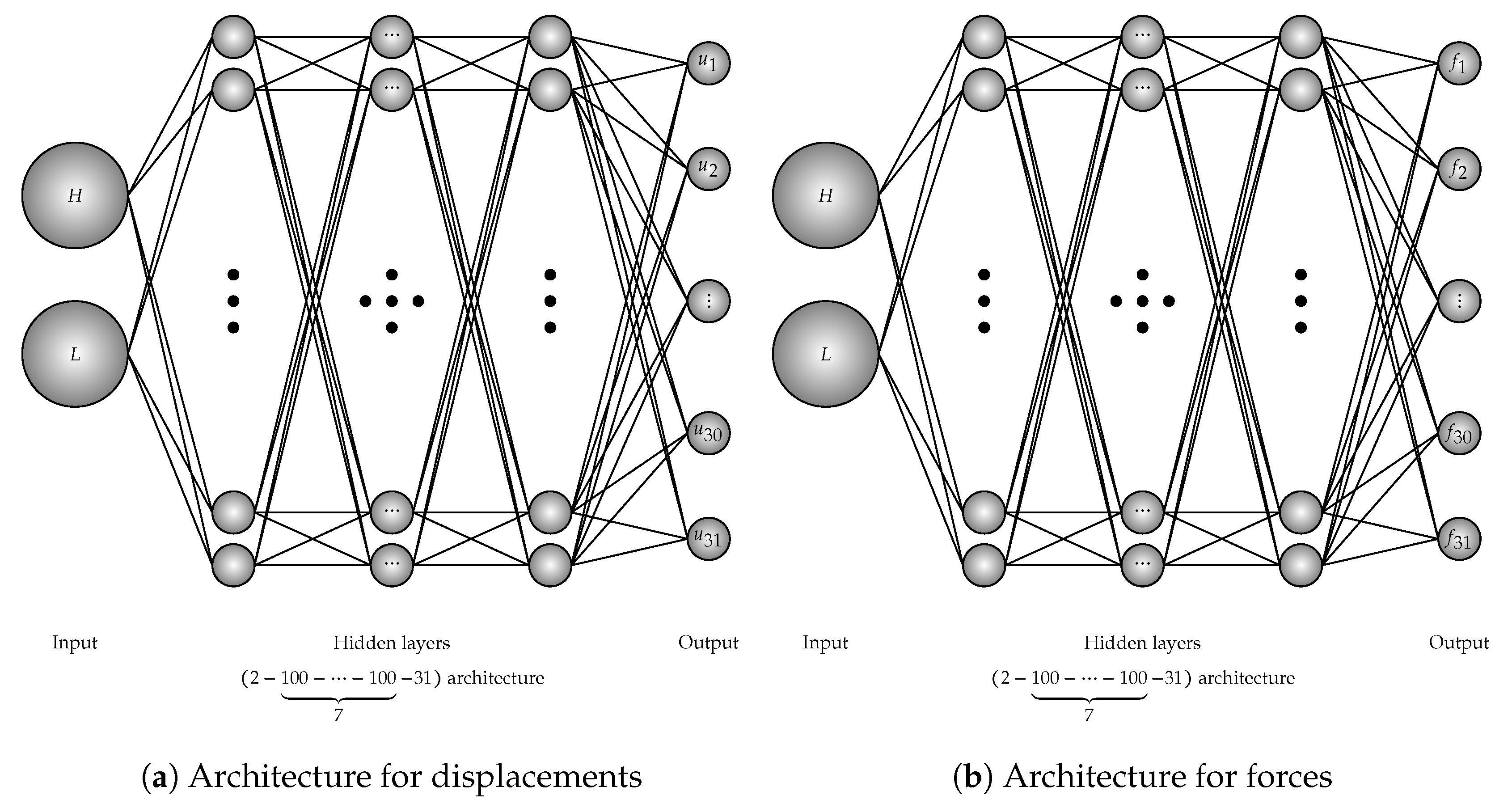
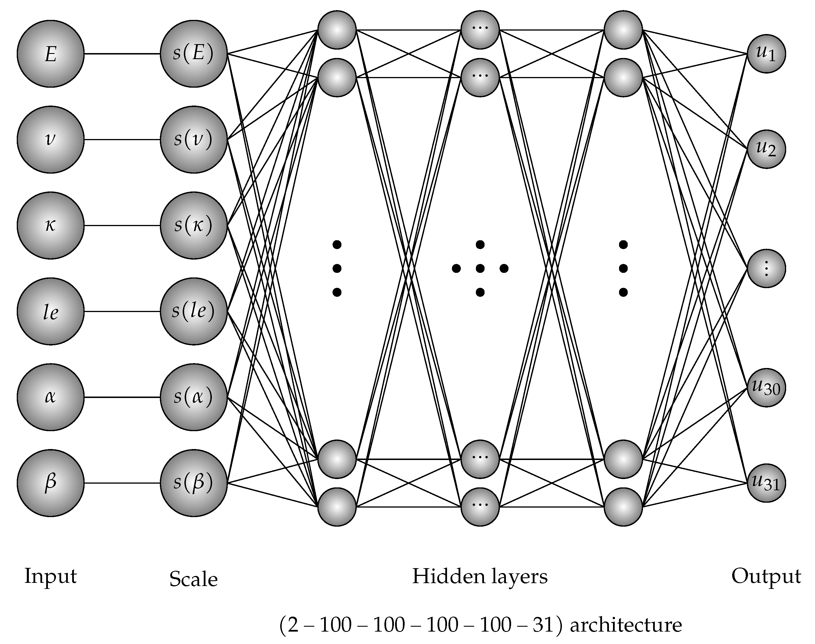
We reconsider the three-point bending specimen that was subjected to an external force f whose various geometry and boundary condition of the specimen are shown in Figure 6. The thickness h of the beam is $0.05$ m and plane stress conditions are assumed. The input of the process are dimensional vectors $\left[H,L\right]$ where $H\in \left[0.1,0.4\right]$ is the height and $L\in \left[1.0,2.3636\right]$ is the length of the specimen. The data will be created by 156 different dimensional vectors where the heights H are linearly generated 12 times while the lengths L are created 13 times. The number of training data is 150 and six data for testing. In this example, to avoid the sensitivity of the data where the displacements $u\in \left[0.1,0.8\right]$ and the forces can exceed 2500, the training process will be separated into two parts. One for displacement and one for forces whose architectures are illustrated in Figure 7. For each input, the vector of output is represented by ${[u_1,\cdots ,u_{31}]}^T$ for displacements and ${[f_1,\cdots ,f_{31}]}^T$ for forces which $(u_i,f_i)$$\forall i=1,\cdots ,31$ are points of loading deflection curve. Therefore, the matrix of output is a $31\times 150$ matrix. The training data will be collected by the gradient-enhanced damage models and the training process based on $(2-\underset{7}{\underbrace{100-\cdots -100}}-31)$ architecture.

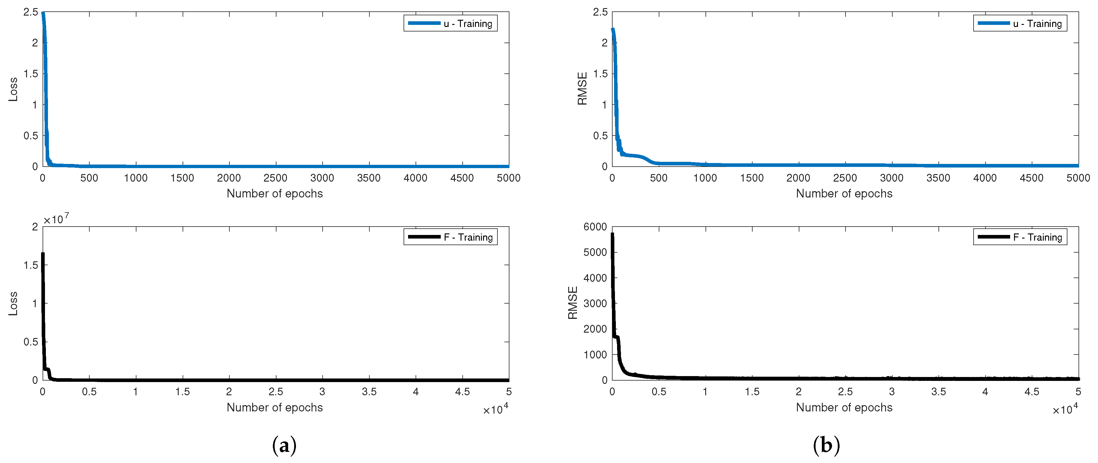
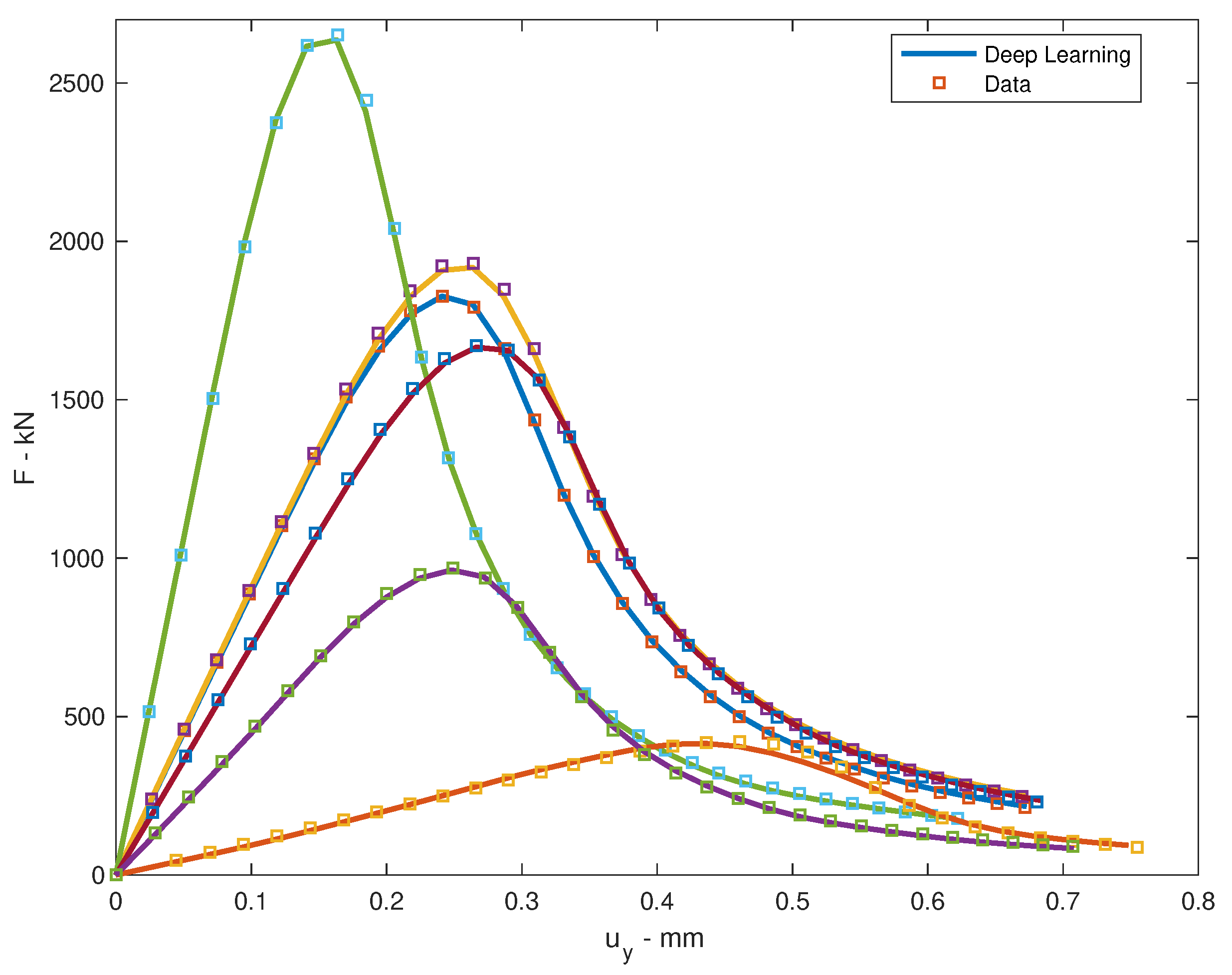
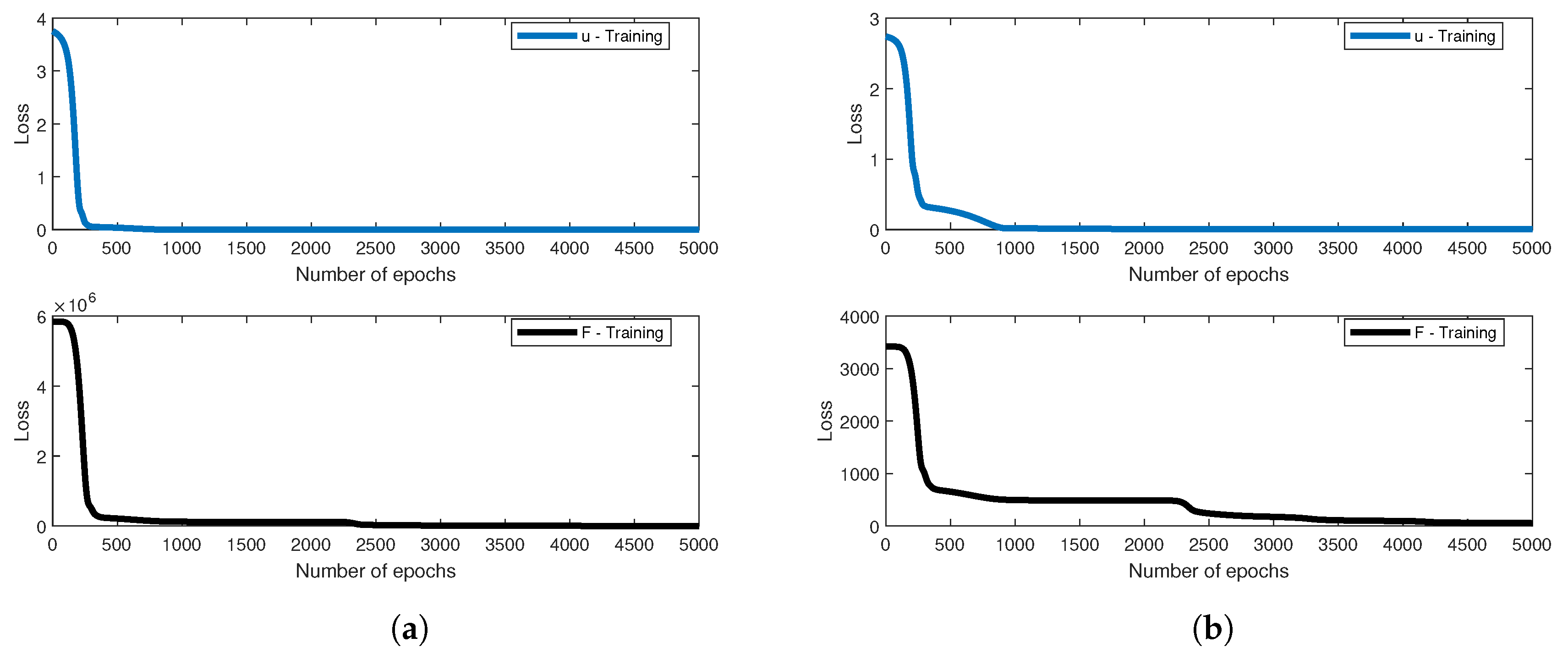
The problem was trained by Adam optimizer by the employment of Rectified Linear Unit (ReLU) activation function with back propagation algorithm. The learning rate of the displacement data is ${\eta }_u={10}^{-3}$ and of the force data is ${\eta }_f=2·{10}^{-3}$. The learning rate drop period is 100 epochs. The learning rate drop factor is $99\%$ for displacement training process and is $99.9\%$ for force training process. The squared gradient decay factor is $0.99$. The gradient decay factor is $0.95$. The size of mini-batch is 100 and the total of epochs is $50,000$ for force - training and is 5000 for displacement-training. The training processes are illustrated in Figure 8. Six data were chosen randomly for testing. The loss values are computed by root mean square error (RMSE) and by mini-batch loss (Loss) for comparison in

Table 4. Loss values for both displacement and forces training in dimensional problem.

Data	RMSE	Mini-Batch Loss
Displacements	$0.0106$	$5.6221\times {10}^{-5}$
Forces	$44.6711$	$997.7515$

. The testing of loading deflection curves by deep learning after train and by data are illustrated in Figure 9.

5.2. Material Parameter Problem

The three-point bending specimen is subjected to an external force f whose geometry and boundary condition of the specimen are shown in Figure 2. In this problem, the force is placed at the middle of the specimen. The thickness h of the beam is $0.05$ m and plane stress conditions are assumed. The input of the process is material parameter vector $\left[E,\nu ,\kappa ,le,\alpha ,\beta \right]$ where E is the Young’s modulus, $\nu$ is the Poisson’s ratio, $\kappa$ is the critical value of equivalent strain, $le$ is the characteristic length and $\alpha$, $\beta$ are softening parameters. The data is created by 4096 different parameter vectors where the parameters are taken in intervals based on the experienced average values in

Table 5. The experienced average value and the range of material parameters.

Parameters	Average	Range
E	$30\times {10}^9$	$\left[25\times {10}^9,35\times {10}^9\right]$
$\nu$	$0.2$	$\left[0.17,0.23\right]$
$\kappa$	$1.1\times {10}^{-4}$	$\left[8\times {10}^{-5},1.4\times {10}^{-4}\right]$
$le$	${10}^{-2}$	$\left[0.005,0.015\right]$
$\alpha$	$0.99$	$\left[0.96,0.99999\right]$
$\beta$	1800	$\left[1600,2000\right]$

. In this example, to avoid the sensitivity of the data where the displacements $u\in \left[0.1,0.8\right]$ and the forces can exceed 1400, and the training process is separated into two parts. One for displacements and one for forces whose architectures are similarly and illustrated in Figure 10. For each input, the vector of output is represented by ${[u_1,\cdots ,u_{31}]}^T$ for displacements, ${[f_1,\cdots ,f_{31}]}^T$ for forces, and $(u_i,f_i)$$\forall i=1,\cdots ,31$ for points of the loading deflection curve. Therefore, the matrix of output is a $31\times 4096$ matrix. The training data are collected by the gradient-enhanced damage models where the training process based on $(2-\underset{4}{\underbrace{100-\cdots -100}}-31)$ architecture for both displacement and force - training.

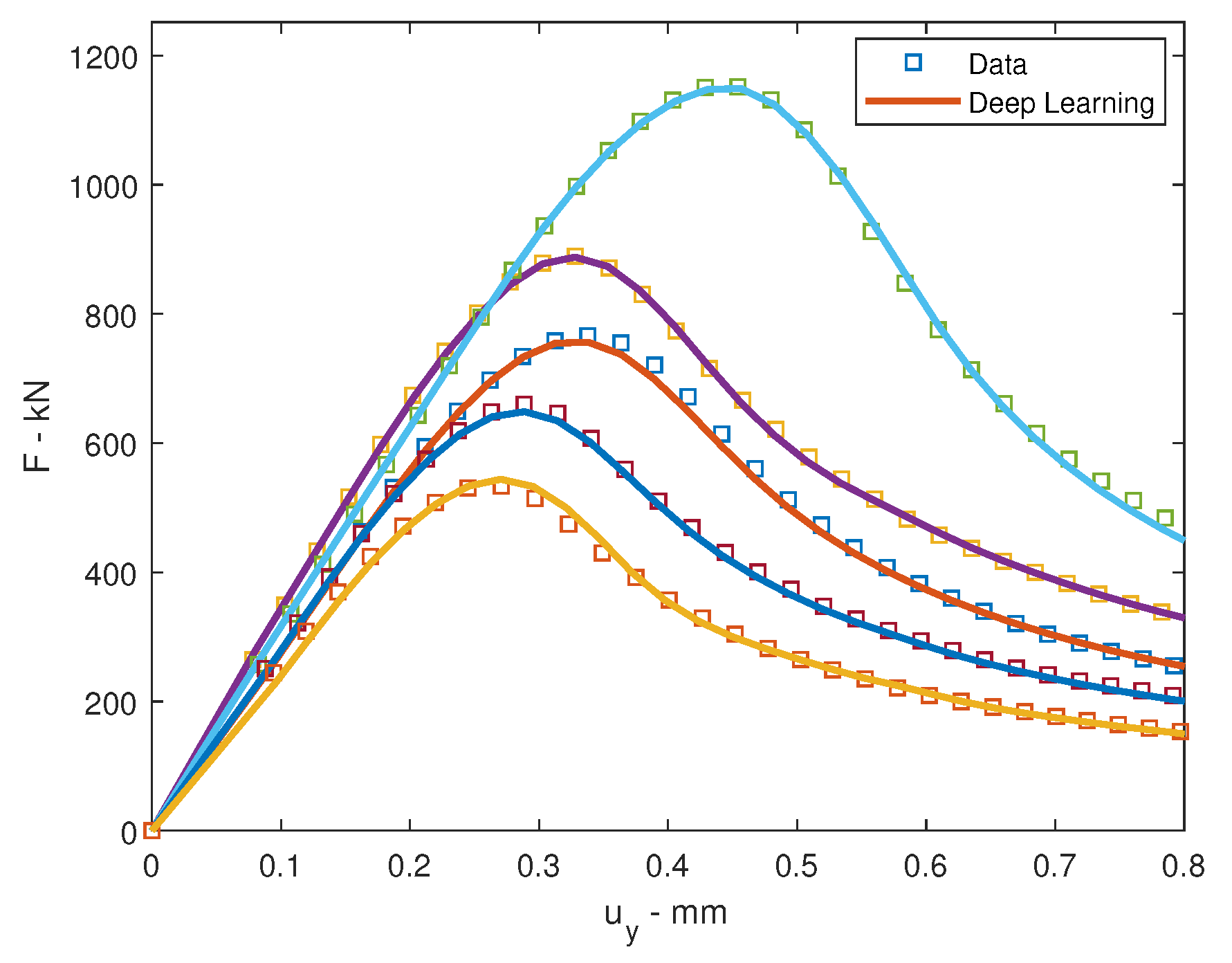
The problem was trained by Adam optimizer by the employment of Rectified Linear Unit (ReLU) activation function with back propagation algorithm. The learning rate of the displacement data is ${\eta }_u={10}^{-4}$ and of the force data is ${\eta }_f=3\times {10}^{-4}$. The learning rate drop period is 100 epochs. The learning rate drop factor is $99\%$. The squared gradient decay factor is $0.99$. The gradient decay factor is $0.95$. The size of the mini-batch is 100 and the total of epochs is 5000. The training processes are illustrated in Figure 11. Six data were chosen randomly for testing. The loss values will be computed by root mean square error (RMSE) and by mini-batch loss (Loss) for comparison in

Table 6. Loss values for both displacement and forces training in material problem.

Data	RMSE	Mini-Batch Loss
Displacements	$7.386\times {10}^{-3}$	$2.728\times {10}^{-5}$
Forces	$54.996$	$1.512\times {10}^3$

. The testing of loading deflection curves by deep learning after training and by data are illustrated in Figure 12.

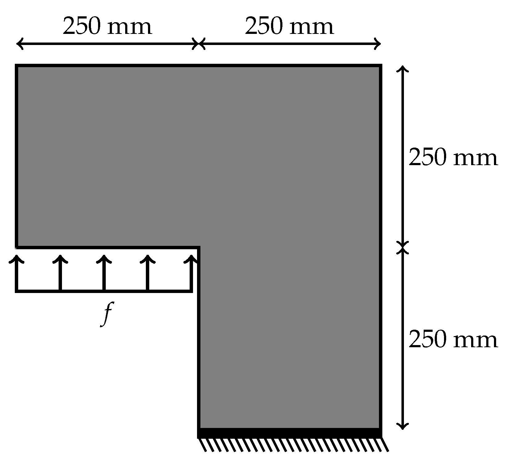
5.3. L-Shape Specimen

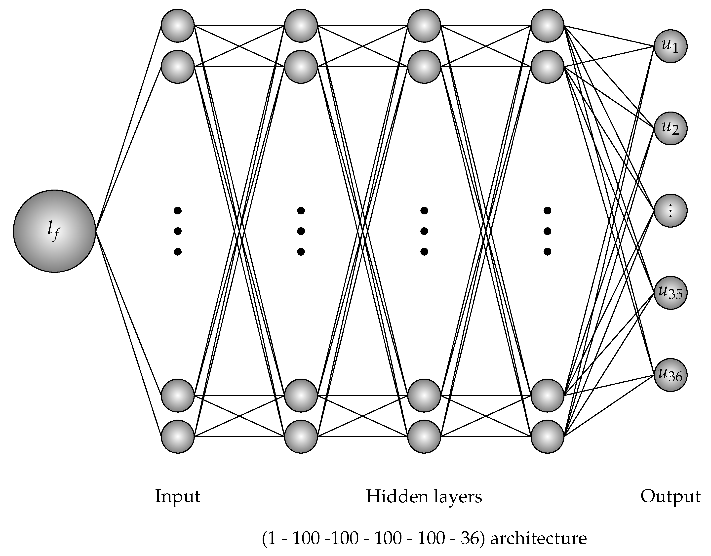
The last example is an L-shaped specimen subjected to a distributed load as shown in Figure 13, which is also a classical benchmark problem used for instance to demonstrate the performance of Isogeometric Analysis (IGA) [37]. The thickness of the specimen is 20 cm and plane stress conditions are assumed. The material parameters are: Young’s modulus $E=10$ (GPa) and Poisson’s ratio $\nu =0.2$. The effective strain in Equation (6) and the damage law in Equation (5) are used with parameters ${\kappa }_0=4\times {10}^{-4}$, $\alpha =0.98$ and $\beta =80$. The non-local length scale is taken as $l_c=5\sqrt{2}\approx 7.07$ (mm). The input of the training process are locations $l_f$ on which the force f is applied. These locations are created by 123 different positions from 0 to ${\mathsf{\Delta }}_p$ where ${\mathsf{\Delta }}_p$ is the span of the various forces. In this example, to avoid the sensitivity of the data where the displacements $u\in \left[0,3\right]$ and the forces can be more than 15000, the training process will be separated into two parts. One for displacements and one for forces whose architectures are illustrated in Figure 14. For each input, the vector of output is formed by ${[u_1,\cdots ,u_{36}]}^T$ for displacements and ${[f_1,\cdots ,f_{36}]}^T$ for forces which $(u_i,f_i)$$\forall i=1,\cdots ,36$ are points of loading deflection curve. Therefore, the matrix of output is a $36\times 5000$ matrix. The training data are collected by the gradient-enhanced damage models where the training process based on $(2-\underset{4}{\underbrace{100-\cdots -100}}-36)$ architecture for displacement-training and $(2-\underset{4}{\underbrace{100-\cdots -100}}-36)$ architecture for force-training.

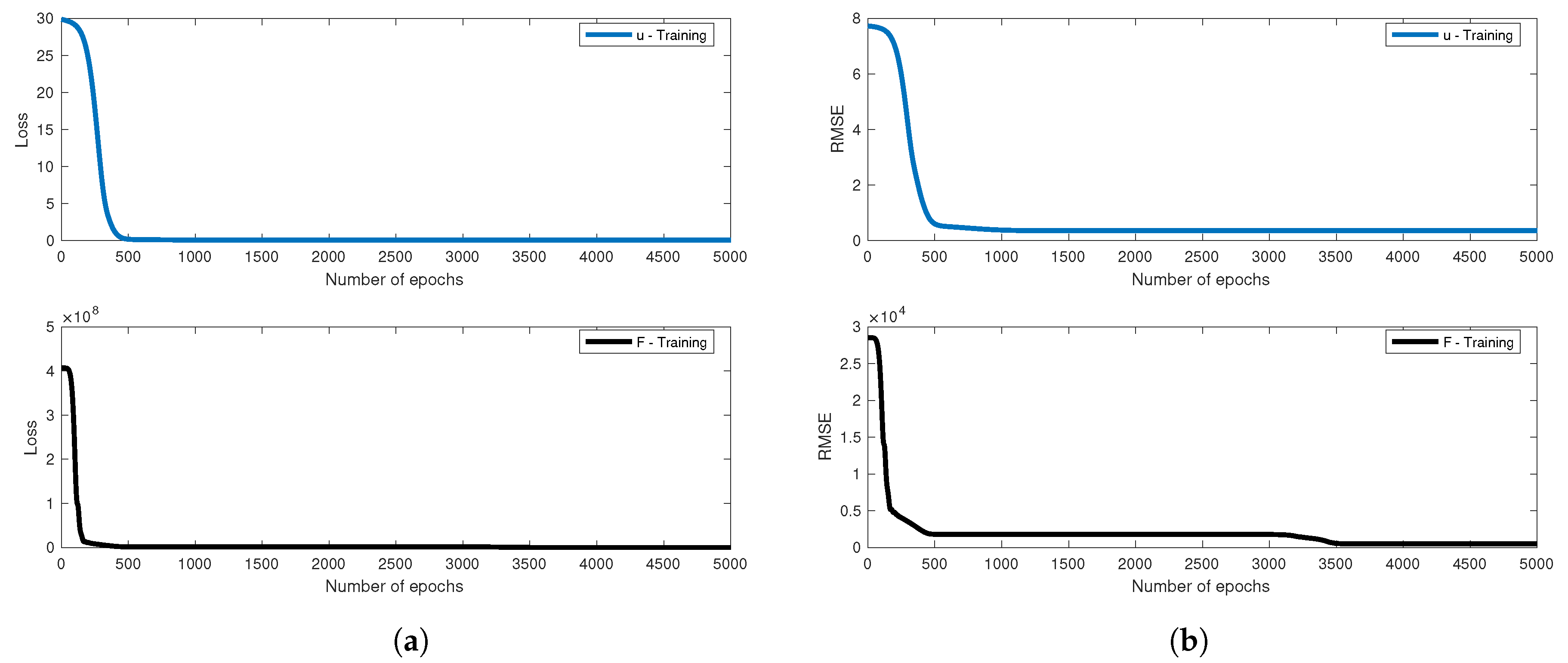
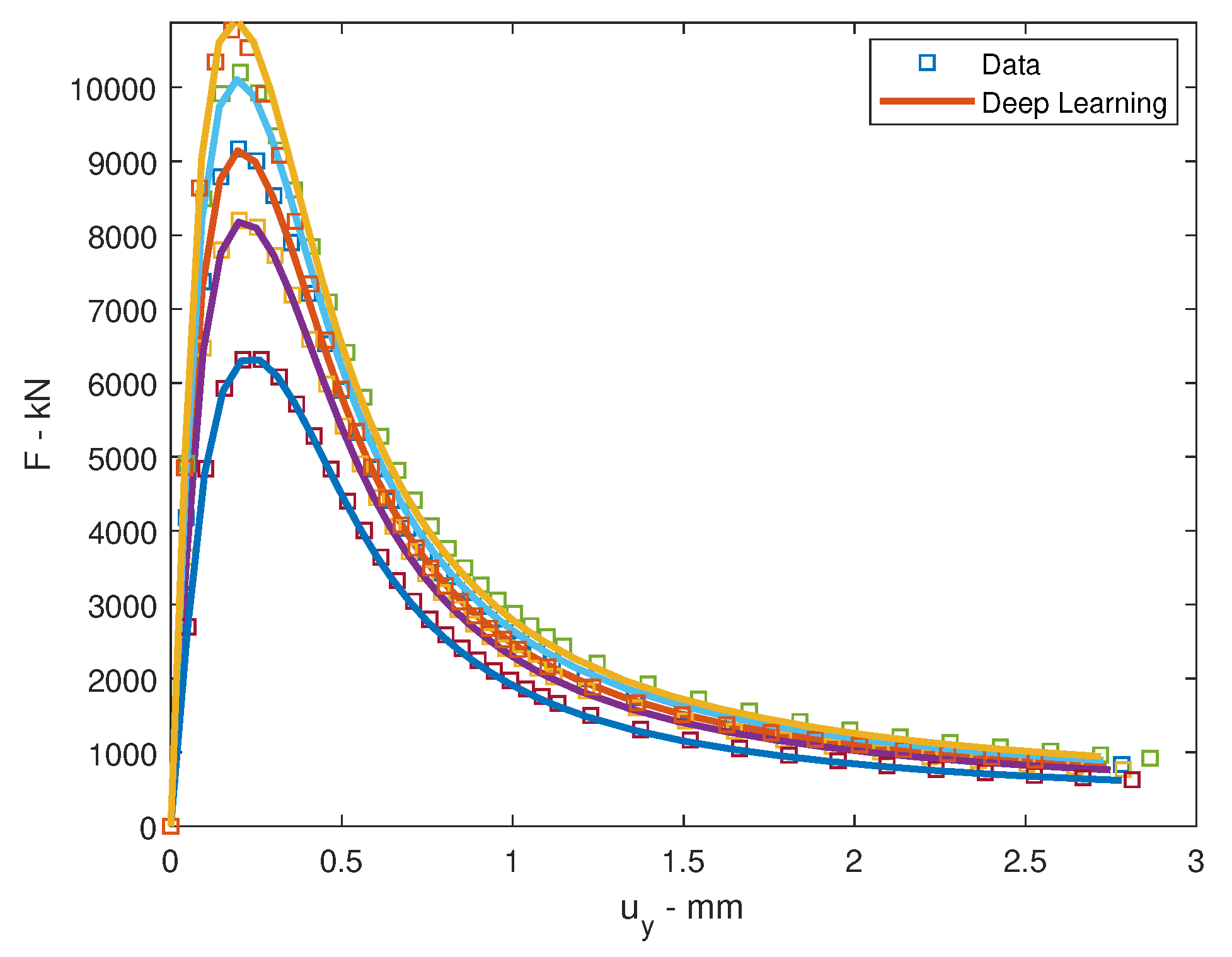
The problem was trained by Adam optimizer by the employment of Rectified Linear Unit (ReLU) activation function with back propagation algorithm. The learning rate of the displacement data is ${\eta }_u={10}^{-4}$ and of the force data is ${\eta }_f=2\times {10}^{-3}$. The learning rate drop period is 100 epochs. The learning rate drop factor is $99\%$. The squared gradient decay factor is $0.99$. The gradient decay factor is $0.95$. The size of mini-batch is 100 and the total of epochs is 5000. The training processes are illustrated in Figure 15. Five randomly data were chosen for testing. The loss values are computed by root mean square error (RMSE) and by mini-batch loss (Loss) for comparison in

Table 7. Loss values for both displacement and forces training in L-shape problem.

Data	RMSE	Mini-Batch Loss
Displacements	$0.36$	$6.4\times {10}^{-2}$
Forces	$479.18$	$\mathrm{114,809.0}$

. The testing of loading deflection curves by deep learning after training and by data are illustrated in Figure 16.

6. Conclusions

This paper introduced a deep learning technique in the context of artificial neural networks for predicting loading deflection curves of structures under gradient-enhanced damage responses. The neural network has been trained based on finite element simulations. We conducted our approach in the form of numerical experiments, using various shapes of specimen as well as inputs. The predictions based on material changes are much more challenging and the number of input parameters will trigger big data in the training phase. The Adam optimizer and Rectified Linear Unit activation function produced the best result for training. The major contribution of this study is to integrate deep learning into computational mechanics. The key feature is how to choose training parameters and deep neural network architecture. Our research is potentially competent for application to a wide range of complex practical engineering problems. In the next step, we intend to develop and apply sufficient transfer learning algorithms, which is important for computational efficiency.

References

- Hinton, G.E.; Osindero, S.; Teh, Y.W. A fast learning algorithm for deep belief nets. Neural Comput. 2006, 18, 1527–1554. [Google Scholar] [CrossRef] [PubMed]
- Nair, V.; Hinton, G.E. Rectified linear units improve restricted boltzmann machines. In Proceedings of the 27th International Conference on Machine Learning (ICML-10), Haifa, Israel, 21–24 June 2010; pp. 807–814. [Google Scholar]
- Hinton, G.E.; Srivastava, N.; Krizhevsky, A.; Sutskever, I.; Salakhutdinov, R.R. Improving neural networks by preventing co-adaptation of feature detectors. arXiv 2012, arXiv:1207.0580. [Google Scholar]
- LeCun, Y.; Bengio, Y.; Hinton, G. Deep learning. Nature 2015, 521, 436. [Google Scholar] [CrossRef]
- Adeli, H. Neural networks in civil engineering: 1989–2000. Comput. Aided Civ. Infrastruct. Eng. 2001, 16, 126–142. [Google Scholar] [CrossRef]
- Deo, R.C. Machine learning in medicine. Circulation 2015, 132, 1920–1930. [Google Scholar] [CrossRef] [PubMed] [Green Version]
- Angermueller, C.; Pärnamaa, T.; Parts, L.; Stegle, O. Deep learning for computational biology. Mol. Syst. Biol. 2016, 12, 878. [Google Scholar] [CrossRef]
- Park, Y.; Kellis, M. Deep learning for regulatory genomics. Nat. Biotechnol. 2015, 33, 825. [Google Scholar] [CrossRef]
- Goh, G.B.; Siegel, C.; Vishnu, A.; Hodas, N.O.; Baker, N. Chemception: A deep neural network with minimal chemistry knowledge matches the performance of expert-developed qsar/qspr models. arXiv 2017, arXiv:1706.06689. [Google Scholar]
- Ravì, D.; Wong, C.; Deligianni, F.; Berthelot, M.; Andreu-Perez, J.; Lo, B.; Yang, G.Z. Deep learning for health informatics. IEEE J. Biomed. Health Inf. 2017, 21, 4–21. [Google Scholar] [CrossRef] [Green Version]
- Samaniego, E.; Anitescu, C.; Goswami, S.; Nguyen-Thanh, V.M.; Guo, H.; Hamdia, K.; Zhuang, X.; Rabczuk, T. An energy approach to the solution of partial differential equations in computational mechanicsvia machine learning: Concepts, implementation and applications. Comput. Methods Appl. Mech. Eng. 2020, 362, 112790. [Google Scholar] [CrossRef] [Green Version]
- Furukawa, T.; Yagawa, G. Implicit constitutive modelling for viscoplasticity using neural networks. Int. J. Numer. Methods Eng. 1998, 43, 195–219. [Google Scholar] [CrossRef]
- Lefik, M.; Boso, D.; Schrefler, B. Artificial neural networks in numerical modelling of composites. Comput. Methods Appl. Mech. Eng. 2009, 198, 1785–1804. [Google Scholar] [CrossRef]
- Rafiee, R.; Habibagahi, M.R. Evaluating mechanical performance of GFRP pipes subjected to transverse loading. Thin-Walled Struct. 2018, 131, 347–359. [Google Scholar] [CrossRef]
- Rafiee, R.; Torabi, M.A. Stochastic prediction of burst pressure in composite pressure vessels. Compos. Struct. 2018, 185, 573–583. [Google Scholar] [CrossRef]
- Rafiee, R.; Torabi, M.A.; Maleki, S. Investigating structural failure of a filament-wound composite tube subjected to internal pressure: Experimental and theoretical evaluation. Polym. Test. 2018, 67, 322–330. [Google Scholar] [CrossRef]
- Ghaboussi, J.; Pecknold, D.A.; Zhang, M.; Haj-Ali, R.M. Autoprogressive training of neural network constitutive models. Int. J. Numer. Methods Eng. 1998, 42, 105–126. [Google Scholar] [CrossRef]
- Oeser, M.; Freitag, S. Modeling of materials with fading memory using neural networks. Int. J. Numer. Methods Eng. 2009, 78, 843–862. [Google Scholar] [CrossRef]
- Ootao, Y.; Kawamura, R.; Tanigawa, Y.; Imamura, R. Optimization of material composition of nonhomogeneous hollow sphere for thermal stress relaxation making use of neural network. Comput. Methods Appl. Mech. Eng. 1999, 180, 185–201. [Google Scholar] [CrossRef]
- Gawin, D.; Lefik, M.; Schrefler, B. ANN approach to sorption hysteresis within a coupled hygro-thermo-mechanical FE analysis. Int. J. Numer. Methods Eng. 2001, 50, 299–323. [Google Scholar] [CrossRef]
- Yun, G.J.; Ghaboussi, J.; Elnashai, A.S. Self-learning simulation method for inverse nonlinear modeling of cyclic behavior of connections. Comput. Methods Appl. Mech. Eng. 2008, 197, 2836–2857. [Google Scholar] [CrossRef]
- Lee, S.; Ha, J.; Zokhirova, M.; Moon, H.; Lee, J. Background Information of Deep Learning for Structural Engineering. Arch. Comput. Methods Eng. 2018, 25, 121–129. [Google Scholar] [CrossRef]
- Mazars, J.; Pijaudier-Cabot, G. Continuum damage theory—Application to concrete. J. Eng. Mech. 1989, 115, 345–365. [Google Scholar] [CrossRef]
- Peerlings, R.; De Borst, R.; Brekelmans, W.; Geers, M. Gradient-enhanced damage modelling of concrete fracture. Mech. Cohesive-Frict. Mater. Int. J. Exp. Model. Comput. Mater. Struct. 1998, 3, 323–342. [Google Scholar] [CrossRef]
- De Vree, J.; Brekelmans, W.; Van Gils, M. Comparison of nonlocal approaches in continuum damage mechanics. Comput. Struct. 1995, 55, 581–588. [Google Scholar] [CrossRef] [Green Version]
- Peerlings, R.H.J.; De Borst, R.; Brekelmans, W.A.M.; De Vree, J. Gradient enhanced damage for quasi-brittle materials. Int. J. Numer. Methods Eng. 1996, 39, 3391–3403. [Google Scholar] [CrossRef]
- Bazant, Z.P.; Pijaudier-Cabot, G. Nonlocal continuum damage, localization instability and convergence. J. Appl. Mech. 1988, 55, 287–293. [Google Scholar] [CrossRef]
- Lasry, D.; Belytschko, T. Localization limiters in transient problems. Int. J. Solids Struct. 1988, 24, 581–597. [Google Scholar] [CrossRef]
- De Borst, R.; Mühlhaus, H.B. Gradient-dependent plasticity: Formulation and algorithmic aspects. Int. J. Numer. Methods Eng. 1992, 35, 521–539. [Google Scholar] [CrossRef] [Green Version]
- Schreyer, H.L.; Chen, Z. One-dimensional softening with localization. J. Appl. Mech. 1986, 53, 791–797. [Google Scholar] [CrossRef]
- Triantafyllidis, N.; Aifantis, E.C. A gradient approach to localization of deformation. I. Hyperelastic materials. J. Elast. 1986, 16, 225–237. [Google Scholar] [CrossRef]
- Bažant, Z.P.; Pijaudier-Cabot, G. Measurement of characteristic length of nonlocal continuum. J. Eng. Mech. 1989, 115, 755–767. [Google Scholar] [CrossRef] [Green Version]
- MuĻhlhaus, H.; Aifantis, E. A variational principle for gradient principle. Int. J. Solids Struct. 1991, 28, 845–857. [Google Scholar] [CrossRef]
- Nesterov, Y. Gradient methods for minimizing composite objective function. Math. Program. 2013, 140, 125–161. [Google Scholar] [CrossRef]
- Kingma, D.P.; Ba, J. Adam: A method for stochastic optimization. arXiv 2014, arXiv:1412.6980. [Google Scholar]
- Rumelhart, D.E.; Hinton, G.E.; Williams, R.J. Learning representations by back-propagating errors. Nature 1986, 323, 533. [Google Scholar] [CrossRef]
- Kuhl, K. Numerical Models for Cohesive Frictional Materials. Ph.D. Thesis, Stuttgart University, Stuttgart, Germany, 2000. [Google Scholar]
Figure 1.
Activation function role in deep neural network.
Figure 2.
The various forces with respect to the location in three-point bending specimen.
Figure 3.
Deep neural network architecture for various location forces problem.
Figure 4.
The training process for location-force data in three-point bending specimen.
Figure 5.
The testing of loading deflection curves for location-force problem.
Figure 6.
The various dimension for three-point bending specimen.
Figure 7.
Deep neural network architecture for dimensional problem of the three-point bending specimen.
Figure 8.
The training process for dimensional problem in the three-point bending specimen. (a) Mini-batch loss for dimensional training process; (b) RMSE for dimensional training process.
Figure 9.
The testing of loading deflection curves for dimensional problem.
Figure 10.
Deep neural network architecture for material parameter problem of the three-point bending specimen.
Figure 11.
The training process for material problem in the three-point bending specimen. (a) Mini-batch loss for material training process; (b) RMSE for material training process.
Figure 12.
The testing of loading deflection curves for material problem.
Figure 13.
The various forces with respect to the location in L-shape specimen.
Figure 14.
Deep neural network architecture for force locations problem of the L-shape specimen.
Figure 15.
The training process for shear force problem in the L-hape specimen. (a) Mini-batch loss for L-shape shear force training process; (b) RMSE for L-hape shear force training process.
Figure 16.
The testing of loading deflection curves for L-hape problem.