Some Algorithms to Solve a Bi-Objectives Problem for Team Selection

Abstract

In real life, many problems are instances of combinatorial optimization. Cross-functional team selection is one of the typical issues. The decision-maker has to select solutions among $\left(\begin{array}{c}k\\ h\end{array}\right)$ solutions in the decision space, where k is the number of all candidates, and h is the number of members in the selected team. This paper is our continuing work since 2018; here, we introduce the completed version of the Min Distance to the Boundary model (MDSB) that allows access to both the “deep” and “wide” aspects of the selected team. The compromise programming approach enables decision-makers to ignore the parameters in the decision-making process. Instead, they point to the one scenario they expect. The aim of model construction focuses on finding the solution that matched the most to the expectation. We develop two algorithms: one is the genetic algorithm and another based on the philosophy of DC programming (DC) and its algorithm (DCA) to find the optimal solution. We also compared the introduced algorithms with the MIQP-CPLEX search algorithm to show their effectiveness.

1. Introduction

1.1. Background

This research was the continuing work we started since 2018 [1] and 2019 [2] when we tasked with recruiting a group of students to participate in the international programming contest for students (ACM-ICPC). We have to select h candidates from many potential candidates in the school. A group chosen simply by selecting those who have the highest total score is a lack. Many team members tend to be good at the same skill. The selection method may make their weaknesses easy to exploit, while their strengths become redundant. The selected team must be not only skillful, but also cross-functions. In management science, there are many types of teams that have been defined and used. However, the cross-functional team seems to be the most suitable form for the expected group, where candidates have many different skills and can support each other. Many ideas help our point of view; for example, Keller believes that cross-functional teams consist of members of different functional areas, such as engineering, manufacturing, or marketing. Cross-functional makeup provides the advantages of multiple sources of information and perspectives [3]. The role of the cross-functional team in using the expertise of many different people, coupled with the task of enlisting support for the work of the group [4]. The training practice history of the candidates recorded and summarized. This data were then used to determine the most suitable team as shown in Figure 1.

There is a lot of previous research used binary programming optimization as the decision-making model to indicate the selected candidates. For example: some authors used binary integer programming to select a cricket team [5,6,7]. Usually, the decision variable $x_i$ is used to represent the presence or absence of the ith candidate in the selected team, where $x_i=\{\begin{array}{c}1 if candidate ith is selected\\ 0 otherwise\end{array}$. The problem is a combinatorial optimization with decision space size is $\left(\begin{array}{c}k\\ h\end{array}\right)$. It is not possible to search for all available solutions in the real life application. Thus, there are two tasks to do: to define the search range and to determine the effective search algorithm.

Sandhya et al. [8] have considered the team leader selection problem as the Multi-Criteria Decision Making (MCDM) problem and uses the Euclidean Distance Based Approximation (EDBA) approach to solve the problem. The MCDM analytical approach has chosen to assess the performance of team leaders to make the right choice. The working principle of EDBA focuses on specifying the optimal state of the target represented by the optimal model, i.e., OPTIMAL and ideal values for all selected indexes to consider. Their ideas are very appealing to us, due to the optimal team selection being difficult, but a predefined expectation is possible. The selected members with performance both “wide” and “deep”. The terms “wide” and “deep” mean that the selected teams not only consist of the good candidates but are able to support each other by cross-skills.

In the investigated research, the performance of the selected team can be accessed by the sum of the rating that the team’s members have been achieved. This objective function is defined as: $\max ({\sum }_{i=1}^k{x}_i{\phi }_i)$, where ${\phi }_i$ is the rating value of performance criteria of member $i^{th}$. This objective function will bring you the top candidates, but there is no guarantee that top candidates work well together on the same team due to a shortage of different skills. Two members of the team that are good at graph theory may not be sure of solving problems on the array well. Feng et al. introduced a multiple-objectives to select the most preferred members from available candidates in their departments considering interior and exterior organizational collaborative performance [9]. Fan et al. [10] use a bi-objective optimization to select their R&D team. Su et al. introduced a multi-objective optimization model that considers the individual knowledge competence, knowledge complementarity, and collaboration performance [11]. For the targets that access “deep” and “wide” aspects, the objective of the selection model now can be formulized as a two objectives’ optimization problem [12] as follows:

$$\max (f_1(x)={\sum }_{i=1}^k({\sum }_{j=1}^m{C}_{i,j}\ast x_i)),\max (f_2(x)={\sum }_{i=1}^k({\sum }_{j=1}^m{R}_{i,j}\ast x_i)) (\ast ),$$

where m is the number of available skills, and $f_1(x)$ represents the number of skills that the team is proficient in (wide). $f_2(x)$ stands for the total score (deep) archived by the selected team. $C_{i,j}$ = 1 if member $i^{th}$ has experience on skill $j^{th}$. Denote $R =\{R_{i,j} \ge 0|i = \left\{1,\dots ,k\right\},j = \left\{1,\dots ,m\right\} \}$. $R_{i,j}$ is the score of member $i^{th}$ on skill $j^{th}$.

There are many approaches to solving the (*) problem mentioned in the survey of Hwang [13] such as: (1) scalarizing: that formulating a single-objective optimization problem from the origin multi-objective optimization problem where the new objective function is the sum of the product between the separated objective and its weight parameter. (2) Visualization of the Pareto front: that allows the decision-maker to identify the preferred point at the Pareto front. Most of those methods require consideration of the decision-maker to select parameters about the importance of each objective-function in the decision space. This may be difficult for the decision maker in the real life problem. Instead of using those approaches, we use the compromise programming approach.

1.2. Compromise Solution

Zeleny [14] introduced the concept of the ideal solution that defined as the best-compromise solution is the nearest solution concerning perfection, accepting the fundamental postulate that the decision-maker prefers solutions as close as possible to the ideal. In [1], we propose the MDSB model, which uses a similar approach of “A Discrete Approximation of the Best Compromise solution”. The idea of MDSB is to minimize the distance between the selected team and the idea team. The norm 2 metrics used to measure the distances between considered points to optimal solution. We define that E ∈$R^m$ is the expected solution. It does not matter if the available candidates are able to combine to reach the expectation. In [1], we select the best point $E = [E_j| j=1..m]$ such that $E_j$ describes the sum score of h members who have the highest scores for skill $j^{th}$. We set the closest point $O \in R^m$ to E. The optimal solution O describes the sum of practical experience of the team members and expressed as $O=\left[{\sum }_{i=1}^k(R_{i,0}\ast x_i),{\sum }_{i=1}^k(R_{i,1}\ast x_i),\dots ,{\sum }_{i=1}^k(R_{i,m}\ast x_i)\right]$. If we can minimize the distance between O and E, then we get the selected team. The MDSB is defined as follows:

$$\min \left(distance(E,O)=\sqrt{\sum _{j=1}^m{\left(E_j-\sum _{i=1}^k{R}_{i,j}\ast x_i\right)}^2}\right)$$

subject to:

$$x_i=\left\{0,1\right\} \forall i=1..k$$

$$\sum _{i=1}^k{x}_i=h$$

$${\sum }_{i=1}^k(x_i\ast R_{i,j}) \ge z_j \forall j=1..m$$

$${\sum }_{i=1}^k{x}_i\ast c_i \le C$$

Point E represents an ideal squad. The chosen roster only coincides with the perfect team if there are h outstanding members in all areas. Choosing the line-up corresponding to E is very easy when compared to selecting the weights corresponding to the objective functions of the multi-objective optimization problem. In this version, we have added constraints against the version introduced in [1]. $z_j$ in the constraints represent the minimum score of the skill j-th that the selected team must reach (we denote each of them as constraint j-th corresponding to skill j-th). These constraints require the selected group not to be severely deficient in a particular skill. We applied the original model that we used in [1]. It brought us one of our brightest teams, but in the 2019 Vietnamese national northern exam, our select group of 3 did not achieve the expected results due to the weakness of some skills. The ACM-ICPC exam requires a lot of skills, so having a severe deficiency needs to be considered and eliminated. Edmondson and Harvey also emphasize that team members tend to discuss shared knowledge instead of unique knowledge, even if the individual experience is vital to the efforts of their group [15]. In our case, we also clearly see that some of the skills are more common than the others. It is, therefore, essential to require the selected team to satisfy the minimum scores of some traditional skills. C is the maximum cost and $c_i$ is the cost of candidate i-th (we denote this constraint as constraint (m + 1)-th). For students participating in international competitions, we also have scholarship policies for each individual. However, the budget is never infinite, actually for the problem of finding members for the project team. Cost is one of the critical factors for the final decision. The decision-maker can remove one of the not useful constraints to be more suitable to a particular case. We evaluate how these constraints affect the performance of the algorithm.

In [2], we stated that the problem is in the form of mixed integer quadratic programming (MIQP) [16]. The MIQP can be solved by several algorithms such as Genetic algorithm, MIQP-CPLEX, and another effective algorithm inspired from DC and DCA [2]. In this article, we present a tweaking version of the above algorithms and perform experiments with more substantial data to evaluate the algorithms in general.

1.3. Contribution of the Paper

In this study, we describe our continuing work, the MDSB model, to select a cross-functional team that was first introduced since 2018 [1]. The model allows the decision-maker to simultaneously access two “deep” and “wide” aspects when assessing the performance of the selected team. We have conducted closer reviews to supplement our idea of the model. We are also working on improving our model to avoid severe shortages of some skills for the chosen team. The cost for each member was considered in this version of the model. Choosing a good team without the budget is also a significant factor of consideration [4]. The Objective function is not only suitable for ACM-ICPC team selection, but also in many other problems in the form of combination search.

As mentioned in the first part of this paper, the MDSB model is a Mixed-Integer Quadratic Programming (MIQP), which can be directly solved by solvers. In 2019 [2], we developed an algorithm based on the DC and DCA philosophy to solve this model. The algorithm shows superiority when compared to Genetic algorithms (GA) and MIQL-CPLEX (CPLEX). However, the DC modifications for our model were proven and corrected. In this paper, we also add the proof that DC transform is equivalent to the original model, and its DCA algorithm is always capable of convergence. As an additional part of the contribution, the newly added constraints in the model are also carefully evaluated for performance. We redesign a better version of GA for solving the MDSB model and extend the experiments with the larger scale of data and more algorithms.

In the remaining part of this paper, we provide an introduction to DC programming and DCA. Changes and corresponding proofs that covered a better version of GA with a constraint violation checker were introduced as well. The coaching data in our organization are confidential. We do not have the license to publish the data of our students. Therefore, to evaluate the algorithms, we conducted experiments with data obtained from codeforces.com. The remaining are discussion and conclusions.

2. DC Programming and DCA for MDSB

2.1. A Brief Introduction of DC Programming and DCA

DC programming and DCA are for solving the optimization problem of minimizing a function that is a difference of two convex functions on a convex set $C \in R^n$. The general form of a DC program is of the following form: $\inf \left\{f(x)=g(x)-h(x):x\in C\right\},$ where C is a convex set, and $g(x)$ and h(x) are convex functions on C. DC programming and DCA were introduced by Pham Dinh Tao in 1985 and have been extensively developed by both Pham Dinh Tao and Le Thi Hoai An since 1994, see [17] and references therein. The idea of this method is that, instead of solving a nonconvex problem, a sequence of convex sub-problems is solved to find a sequence of solutions that is convergent to the solution of the original problem under some conditions. More specifically, with the initial point $x_0$, a sub problem derived from the original problem by replacing $h(x)$ by its linear approximation at $x_0$ gives the solution $x_1$. This process is repeated until a stopping condition is satisfied. The generic DCA scheme can be described as follows:

• Let $k=0$, Choose $x^k$ in $R^d$, and ϵ is small enough.
• Calculate $y^k$ in $\partial h(x^k)$.
• Calculate $x^{k+1}\in argmin\left\{g(x)-h(x^k)+< x-x^k,y^k >:x\in R^d\right\}.$
• If $|f(x^{k+1})-f(x)|>ϵ ,$ come back to step 2.

Before presenting some essential convergence properties of DCA, it is useful to recall some related notions.

• A vector y is called a subgradient of a convex function f at a point $x^0$ if

  $$f(x)\ge f(x^0)+<x-x^0,y> \forall x.$$

  The set of all subgradients of f at $x^0$ is called the subdifferential of f at $x^0$ and is denoted by $\partial f(x^0)$.
• The modulus of convex function f denoted by

  $$\rho (f)=sup\left\{\rho \ge 0:f-\rho /2.{||.||}^2 is convex\right\}.$$

  If $\rho (f)>0,$ then f is strongly convex.
• A point $x^0$ is called a critical point of $(g-h)$ if it verifies the generalized Kuhn–Tucker condition

  $$\partial g(x^{\ast })\cap \partial h(x^{\ast })\ne \varnothing .$$

  (1)

The convergence of DCA and its basic properties was presented in [17]. Some of the important properties are summarized here:

(i)

The sequences $\left\{g(x^k)-h(x^k)\right\}$ are decreasing and $g(x^k+1)-h(x^k+1)=g(x^k)-h(x^k)$ iff $y^k \in \partial g(x^k) \cap \partial h(x^k),y^k \in \partial g(x^{k+1}) \cap \partial h(x^{k+1})$ and $\left[\rho (g,C)+\rho (h,C)\right]\Vert x^{k+1}-x^k\Vert =0$. Moreover, if g or h are strongly convex on C, then $x^k$ = $x^{k+1}$. In such case, DCA terminates at kth iteration (finite convergence of DCA).

(ii)

If $g(x)$ or $h(x)$ are strongly convex, then the series $\Vert x^{k+1}-x^k\Vert {}^2$ converges.

(iii)

If the optimal value α of DC program is finite and the infinite sequences $\left\{x^k\right\}$ and $\left\{y^k\right\}$ are bounded, then every limit point $x^{\ast }$ of sequence $\left\{x^k\right\}$ is a critical point of $(g-h)$, i.e., $\partial g(x^{\ast })\cap \partial h(x^{\ast }) \ne \varnothing$.

(iv)

DCA has a linear convergence for DC programs.

DC programming and DCA are widely used nowadays due to its efficiency. The success of DCA and its scalability have been shown in a lot of works and in various fields [18,19,20,21].

2.2. DC Decomposition and DCA for MDSB-PMDSB

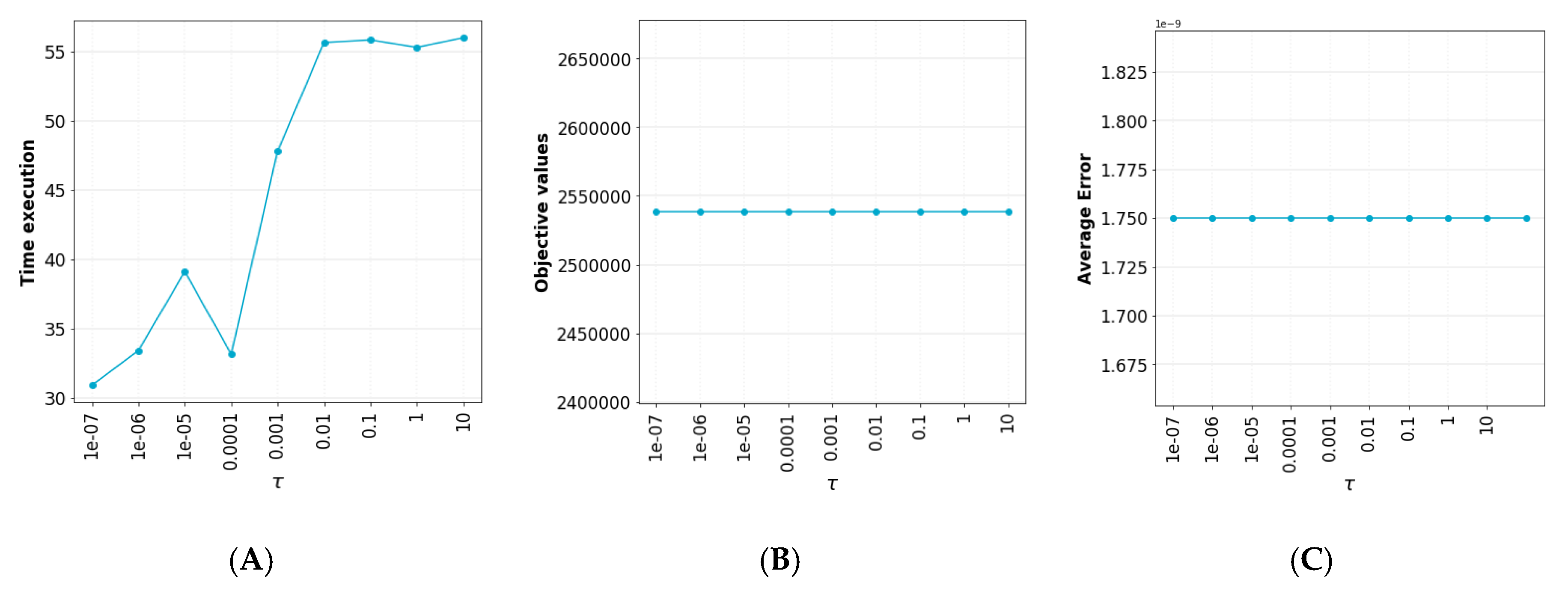
As introduced in [2], the $x_i=\left\{0,1\right\},i=1\dots k$ are non-convex constraints. Le Thi et al. [22] introduced the exact penalty technique to solve the difficulty caused by these constraints. The idea of this technique is that each constraint $x_i=\left\{0,1\right\}$ is first equivalently formulated as:

$$x_i\in \left[0,1\right] \mathrm{and} x_i(1-x_i)\le 0.$$

After that, the constraint $x_i(1-x_i)\le 0$ is penalized to the objective function while still keeping $x_i\in \left[0,1\right]$ as the constraint. As a consequence, the penalized problem with continuous relaxation constraints corresponding to MDSB is given by

$$PMDSB:\min \sum _{j=1}^m{\left(E_j-\sum _{i=1}^k{R}_{ij}{x}_i\right)}^2+\tau \sum _{i=1}^k{x}_i(1-x_i),$$

subject to:

$$x_i\in \left[0,1\right] \forall i=1\dots k$$

$$\sum _{i=1}^k{x}_i=h$$

$${\sum }_{i=1}^k(x_i\ast R_{i,j}) \ge z_j \forall j=1..m$$

$${\sum }_{i=1}^k{x}_i\ast c_i \le C,$$

where τ is a penalty parameter.

It was shown in [2] that both the problems PMDSB and MDSB are equivalent if the penalty parameter τ is appropriately chosen and sufficiently large enough. Thus, we focus on solving the penalized problem PMDSB. It is clear that this problem is not convex since the first term of the objective function ${\sum }_{j=1}^m{(E_j-{\sum }_{i=1}^k{R}_{ij}{x}_i)}^2$ is convex, while the second term ${\sum }_{i=1}^k{x}_i(1-x_i)$ is a concave function. However, it can easily be formed as a DC program: $PMDSB=\min \left\{g(X)-h(X)\right\}$, where both $g(X)=$ ${\sum }_{j=1}^m{(E_j-{\sum }_{i=1}^k{R}_{ij}{x}_i)}^2$ and $h(X)={\sum }_{i=1}^k{x}_i(x_i-1)$ are convex functions on $R^n$. As a result, a DCA scheme can be developed to address the problem PMDSB.

We propose the method to solve this optimization based on a general DC Algorithm:

• Randomly select $X^0=\{x_i^0|0\le x_i^0\le 1\forall i=1\dots k\}$, and ϵ is small enough and a suitable value of τ.
• Calculate the approximation of $h(X)$ at $X^l$.
• Compute $X^{l+1}$ by solving the sub-problem:

  $$\min {\sum }_{j=1}^m{(E_j-{\sum }_{i=1}^k{R}_{ij}{x}_i)}^2-\tau {\sum }_{i=1}^k(2x_i^l-1).x_i,$$

  subject to:

  $$x_i\in \left[0,1\right]\forall i=1\dots k$$

  $$\sum _{i=1}^k{x}_i=h$$

  $${\sum }_{i=1}^k(x_i\ast R_{i,j}) \ge z_j\forall j=1..m$$

  $${\sum }_{i=1}^k{x}_i\ast c_i\le C.$$

  It is possible to solve the problem with several solvers such as CPLEX.
• If $\left||f(X^{l+1})-f(X^l)|\right|/(1+|\mathrm{f}(X^l)|)>ϵ$, come back to step 2.

Although we can guarantee convergence in the infinite limit of l , complete convergence may take a long time in large-scale data, so ε was used as a predetermined bound for obtaining an optimal solution. To make it more convenient for the implementation, we rewrote the sub-problem as a matrix form:

$$\min \frac{1}{2}{X}^{T}AX-b^{T}X,$$

subject to:

$$d^T·X=h$$

$$F·X\le f$$

0 <= X <= 1

where: $A=2R{R}^T$, $b=2RE+\tau (2X^l-1)$, $d={\left[\begin{array}{c}1\\ 1\\ \dots \\ 1\end{array}\right]}_{k\times 1}$, $F={\left[\frac{-R^T}{c_1\dots c_k}\right]}_{(m+1)\times k}$ and $f={\left[\begin{array}{c}{z}_1\\ \dots \\ z_m\\ \mathrm{C}\end{array}\right]}_{(m+1)\times 1}$.

2.3. The Convergence of DCA for PMDSB

It is tractable to realize that the objective function of PMDSB is continuous while the constraint set of PMDSB is closed and bounded. Thus, the optimal value of PMDSB is finite. Furthermore, the second DC component, $h(X)={\sum }_{i=1}^k{x}_i(x_i-1),$ is strongly convex. As a consequence, the convergence of DCA for PMDSB can be straightforwardly deduced from the convergence properties of generic DCA indicated in Section 2.1.

Theorem 1.

Assume that$X^K$is the solution to the sub problem in the kth iteration of DCA for PMDSB.

(i)

The sequence $\{g(X^K)-h(X^k)\}$ is decreasing.

(ii)

The sequence $\left\{||X^{K+1}-X^k|{|}^2\right\}$ is convergent.

(iii)

Every limit point $\left\{X^{\ast }\right\}$ of the sequence $\left\{X^K\right\}$ is a critical point of $(g-h),$ i.e., $\partial g(X^{\ast })\cap$

(iv)

$\partial h(X^{\ast }) \ne \varnothing$.

3. Genetic Algorithm for MDSB

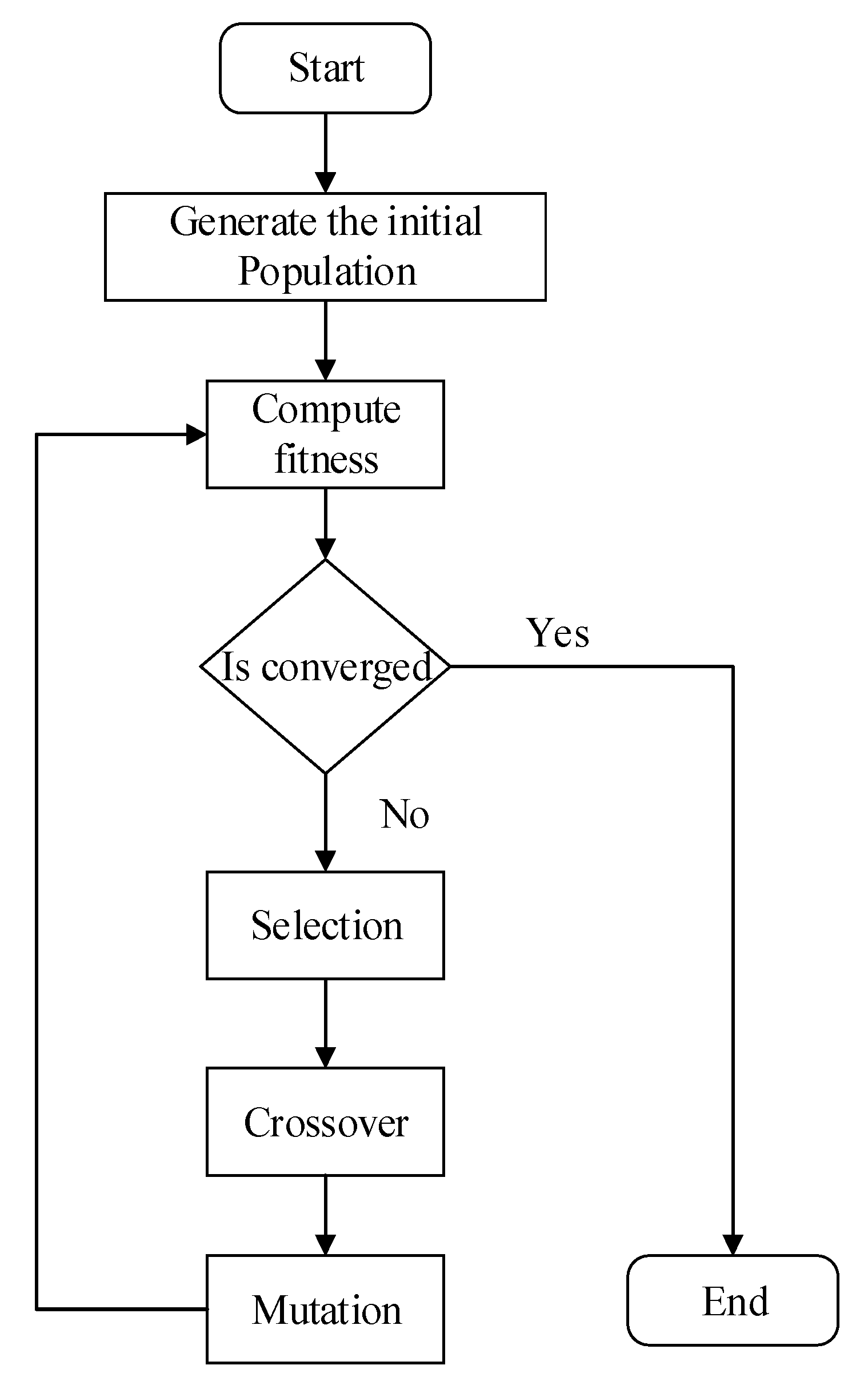
3.1. Introduction to Genetic Algorithm

A genetic algorithm [23] is one of a class of algorithms that searches a solution space for the optimal solution to a problem. This search is done in a fashion that mimics the operation of evolution—a “population” of possible solutions is formed, and new solutions are formed by “breeding” the best solutions from the population’s members to form a new generation. The population evolves for many generations; when the algorithm finishes, the best solution is returned. Genetic algorithms are particularly useful for problems where it is extremely difficult or impossible to get an exact solution, or for difficult problems where an exact solution may not be required. They offer an interesting alternative to the typical algorithmic solution methods and are highly customizable. This notion can be applied to a search problem. We consider a set of solutions for a problem and select the set of best ones out of them. There are five phases that are considered in a genetic algorithm as shown in Figure 2: (1) Generate initial population—a set of individuals are randomly generated. Each individual is a solution to the problem we want to solve. An individual characterized by its gen (a set of variables). (2) The fitness function determines how fit an individual is. The individual that has a higher fitness score has more probability of being selected for the reproduction. (3) Selection—choose the fittest individuals and let them pass their genes to the next generation. (4) Crossover—a crossover point is chosen at random from within the genes for each pair of parents. (5) Mutation—used to maintain genetic diversity from one generation of a population of genetic algorithm chromosomes to the next.

There are several researchers that have designed their own genetic algorithm for solving the mixed binary-integer optimization such as Das [6], Bo Feng et al. [9], Sharp et al. [24], Bhattacharjee and Saikia [7] and Burney et al. [25]. The genetic algorithm is a philosophy, not just a typical algorithm. Therefore, each study has a specific design scheme.

3.2. Genetic Algorithm Scheme for MDSB

Denote $p_i^{(g)}=\left\{p_{i,1}^{(g)},p_{i,2}^{(g)},\dots ,p_{i,h}^{(g)}\right\} \forall i=1\dots D$ as the individual $i^{th}$ in the current iteration g ($g=1$ at the first iteration) and $p_{i,j}^{(g)}$ represents the candidate $j^{th}$ in the team $p_i^{(g)}$. The fitness function is similar to the objective function of the MDSB and denoted as $p_i^{(g)}.fitness=\sqrt{{\sum }_{j=1}^m{(E_j-{\sum }_{i=1}^k{R}_{i,j}\ast x_i)}^2}$. T is a set of characteristics/candidates. G represents the number of generations that have the same fitness value. Our proposed genetic algorithm’s scheme for the MDSB can be described as follows:

• Randomly initialize the populations of k individuals from T.
• Elitism Selection: keep γ as the elitism rate among D individuals that return the best fitness for next-generation. Denote the best fitness value of the ${\mathit{g}}^{\mathit{t}\mathit{h}}$ generation as ${\mathit{b}}^{\mathit{g}}$.
• Crossover: Denote the ω as crossover rate of the D individuals that return the best fitness as K. Randomly select ${\mathit{p}}_{\mathit{f}\mathit{a}\mathit{t}\mathit{h}\mathit{e}\mathit{r}}^{(\mathit{g})}$ and ${\mathit{p}}_{\mathit{m}\mathit{o}\mathit{t}\mathit{h}\mathit{e}\mathit{r}}^{(\mathit{g})}$ from K. We generate the next generation as follows:
  • Set $\mathit{dom}=\mathit{P}(\mathit{dominant}=\mathit{argma}{\mathit{x}}_{\mathit{z}\in \left\{p_{\mathit{father},\mathit{j}}^{(\mathit{g})},{\mathit{p}}_{\mathit{mother},\mathit{j}}^{(\mathit{g})}\right\}}({\sum }_{\mathit{s}=1}^{\mathit{m}}{\mathit{R}}_{\mathit{z},\mathit{s}}))$ is the probability that the candidate dominant selected for the position ${\mathit{j}}^{\mathit{t}\mathit{h}}$ in the ${\mathit{p}}_{\mathit{i}}^{(\mathit{g}+1)}$
  • Set $\mathit{rec}=\mathit{P}(\mathit{recessive}=\left\{{\mathit{p}}_{\mathit{father},\mathit{j}}^{(\mathit{g})},{\mathit{p}}_{\mathit{mother},\mathit{j}}^{(\mathit{g})}\right\}-\left\{\mathit{dominant}\right\}$ is the probability that the candidate recessive selected for the position ${\mathit{j}}^{\mathit{t}\mathit{h}}$ in the ${\mathit{p}}_{\mathit{i}}^{(\mathit{g}+1)}$.
  • Let $\mathit{mut}=\mathit{P}(\mathit{T})$ denote the probability that a random selected candidate in set T chosen for the position ${\mathit{j}}^{\mathit{t}\mathit{h}}$ in the ${\mathit{p}}_{\mathit{i}}^{(\mathit{g}+1)}$. This probability represents the rate of mutation.
  • ${\mathit{p}}_{\mathit{i},\mathit{j}}^{(\mathit{g}+1)}=\mathit{select}(\mathit{dom},\mathit{rec},\mathit{mut}); \forall \mathit{i}=1..(\mathit{D}-(\mathit{D}\ast \mathit{\omega }));\mathit{j}=1..\mathit{h}$
  where $dom+rec+mut=1$ and $select(a,b,c)$ is the function that rolls the dice and returns the corresponding user based on the parameters that are the probabilities passed;
• Constraint validation checking: If there is an individual ${\mathit{p}}_{\mathit{i}}$ that violates any constraints of the MDSB, then it is removed from the set of results.
• Repeat 2, 3, and 4 until ${\mathit{b}}^{\mathit{g}}={\mathit{b}}^{\mathit{g}-1}={\mathit{b}}^{\mathit{g}-2}=\dots ={\mathit{b}}^{\mathit{g}-\mathit{G}}$.

The use of elitism in the selection step at every generation ensures that the best individuals will always be retained. In the current iteration g, choosing $p_{father}^{(g)}$ and $p_{mother}^{(g)}$ in the crossover make a high proportion of better individuals from which p-children is better or equal to its parents. Individuals validated by adding constraints on a minimum score and cost after each crossover step. If any individual does not satisfy the constraints, then it is removed from the current population. This leads the populations of the first generations to not possibly reaching the maximum. However, those who do not meet the constraint gradually decrease in the next generations.

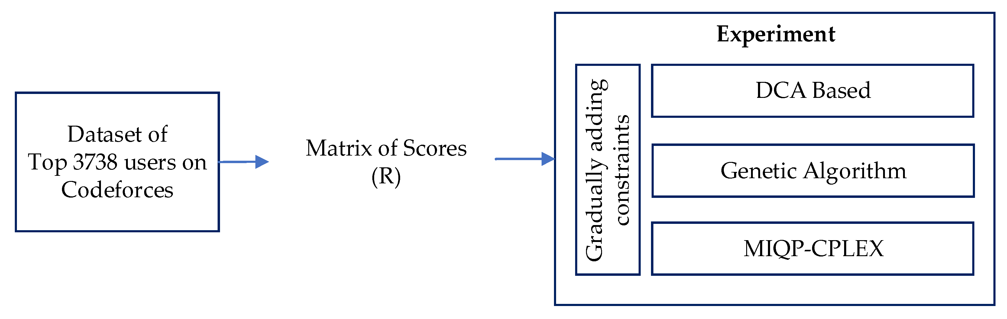
4. Experimental Design

To evaluate the performance of the algorithms on the proposed model, we find the best team of three contestants from the top 3738 high scoring members who come from Southeast Asian countries (k = 3738) on codeforces.com [26]. We proceed to download all the problems they have solved on codeforces.com. It is an automated system to run programming contests. Day by day, their user started the new competitions that allow other users to participate. Figure 3 shows the distribution of the number of members per country (data aggregated on 12 January 2020). It observed that the country with the most members participating in this community is Vietnam with 2329. The countries stand respectively behind are Indonesia, Thailand, and the Philippines. The remaining states have only a small number of members. It reflects their actual results in ACP-ICPC exams held every year.

Every problem uploaded to codeforces.com tagged with one or a few tags as the required skills to solve the problem and defined with the corresponding score. The data are stored as a matrix, where the columns represent the category of the exercises. A single row shows the scores of a particular member. The cell of the matrix describes the total score that the member gained for the corresponding category of the problem, as shown in Figure 4.

There are 37 tags added to the problems that are solved by all members including math, implementation, geometry, bitmasks, brute force, binary search, dp, greedy, chinese remainder theorem, fft, sortings, number theory, constructive algorithms, trees, matrices, divide and conquer, probabilities, dfs and similar, data structures, flows, meet-in-the-middle, games, graphs, shortest paths, hashing, strings, combinatorics, interactive, dsu, graph matchings, two pointers, string suffix structures, 2-sat, expression parsing, * special, ternary search, and schedules. Distribution of total points that users have achieved on each skill shown in Figure 5. The skills have been rearranged in descending order. Skills such as implementation, math, brute forces, and greedy are some of the most common. Figure 6 displays the minimum, maximum, and average score of the skills.

The graphs shown in Figure 7 illustrate the normal distribution of the skills on practical data of all members. The standart distribution function f formulated as $f(x,\mu ,\sigma )=\frac{1}{\sqrt{2\mathsf{\pi }}\sigma }{e}^{-\frac{{(x-\mu )}^2}{2{\sigma }^2}}$, where σ is the standard deviation and μ is the mean. The data are unevenly distributed, focusing more on the left tail and less on the right tail of the curve (collapsed right). This shows that the majority of the points value of the skills are concentrated to the left (less than) average value.

In the proposed model, the first two constraints determine the logic of the model. Therefore, they will always be present when we present the results of the experiment. The remaining 38 constraints (with 37 restrictions on the minimum score for each skill and one limitation on the total cost of the members) are business-related. We proceed to add each constraint to the model to evaluate their impact on the different algorithms. Figure 8 expresses our experimental procedure. The computer we use for the experiment is a maximum configuration for IBM’s free educational purposes: Processor: Intel(R) (City, US State abbrev. if applicable, Country) Xeon(R) CPU X5650 @2.67 GHz (four CPUs), ~2.3 GHz; Memory: 8096 MB RAM; all code implemented in C++ 11.

5. Result

5.1. Init Parameter

The parameters to execute the algorithms are selected by experiments. For the DCA algorithm, the PMDSB model contains the τ as the parameter. We remove all added constraints then run DCA with different values of tau from 10⁻⁶ to 10. In the penalty theory, when the parameter tau becomes large, the solution of the penalized problems approaches that of the original one. However, in practice, the bigger tau is, the slower the speed of algorithms is. Therefore, in this paper, we test with tau varying in a range of values to find a suitable value of tau that is good enough for both theory and practice. We compute the error of the decision variable with the original expectations as: ${\mathrm{e}}_i=\{\begin{array}{cc}1-x_i& if x_i\ge 0.5\\ x_i& otherwise\end{array} \forall i=1\dots 3738$. The detail of objective values, execution times, and average errors $\overline{\mathrm{e}}=\frac{1}{3738}{\sum }_{i=1}^{3738}{\mathrm{e}}_i$, corresponding to different value of τ displayed in Figure 9.

The results show that different values of the τ variable do not affect the returned objective values and average errors of the decision variables of the algorithm with the same initiation points. The processing time for DCA increased slightly proportional to the increasing of τ. τ = 0.01 indicated for further evaluations.

To execute the Genetic Algorithm, we choose the values for the parameters by running the algorithm many times. The genetic algorithm was governed by many different probability values. The model to execute algorithms contains all of the business constraints with 3738 candidates. The team size h = 3. The affections of the Genetic Algorithm’s parameters to the execution time and fitness values summarized from our experiments as follows:

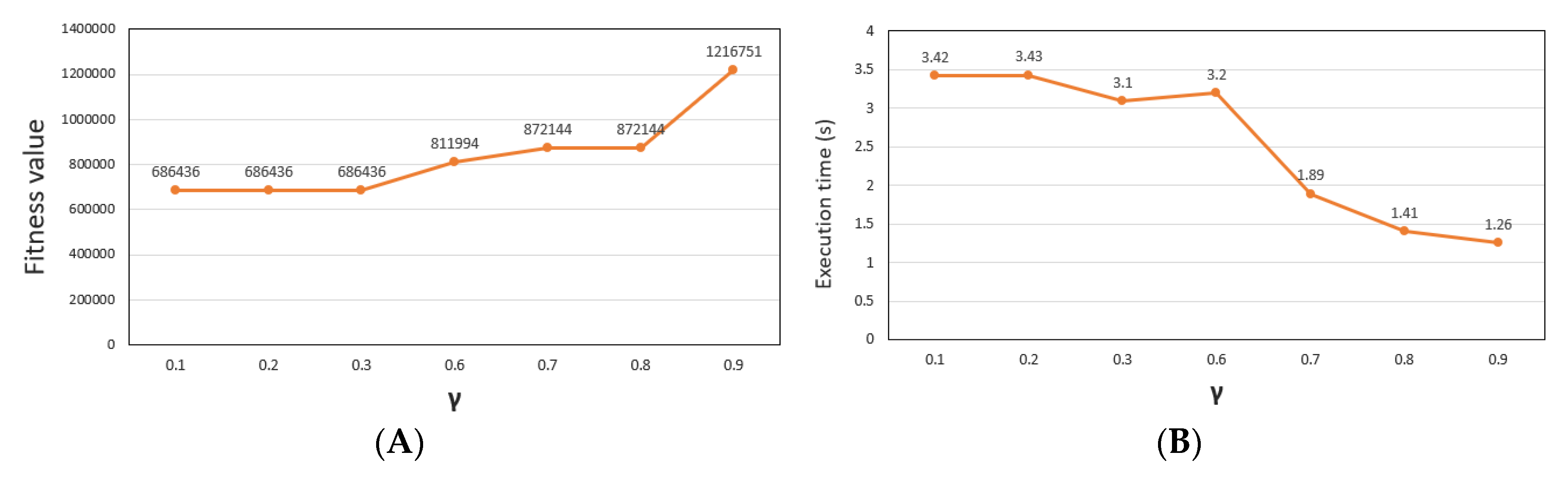
• γ: defined as the rate of individuals remains the same for the next generation. γ = 0.4 to 0.9, the algorithm is fast convergence but generates a not good fitness value. In addition, γ = 0.1 to 0.3 makes the algorithm to have stable convergence, while creating a fitness value. Figure 10 displays the execution and fitness values over generations corresponding to different amounts of γ.
• D: defined as the rate of population size to the whole candidates. The execution time is proportional to the magnitude of D (not significant gap). D takes too small values generating unstable fitness values. D = 0.7 to 0.9 generates more stable fitness values.
• ω: represents the crossover rate. The execution time is proportional to the magnitude of ω (not a significant gap). ω = 0.2 to 0.5 provides relatively stable fitness values. However, there is still a possibility that fitness is not functional because the number of individuals to choose for crossovers shrinks quickly through each generation, leading to a loss of diversity, ultimately making the results worse. ω = 0.6 to 0.9 generates unstable fitness. Because the pool of the crossover is large, it is not good for the improvement of the individuals over generations, which occurs more often when generations > 10.
• $dom, rec, mut$: denote the rates of the selection of recessive, dominant, and mutant genes during the crossover. These parameters are interdependent.

  Table 1. Different pair values of the rates of the selection of recessive, dominant, and mutant genes during the crossover.

  ID	dom	rec	mut	Observation Results
  1	0.7	0.2	0.1	Fast convergence, good, and stable fitness values.
  2	0.6	0.3	0.1	Fast convergence, good and stable fitness values. More stable than pair 1.
  3	0.4	0.4	0.2	Slow convergence, good, and stable fitness values.
  4	0.2	0.7	0.1	Slow convergence, worse, and unstable fitness values.

  shows some performance results relative to the value pairs.

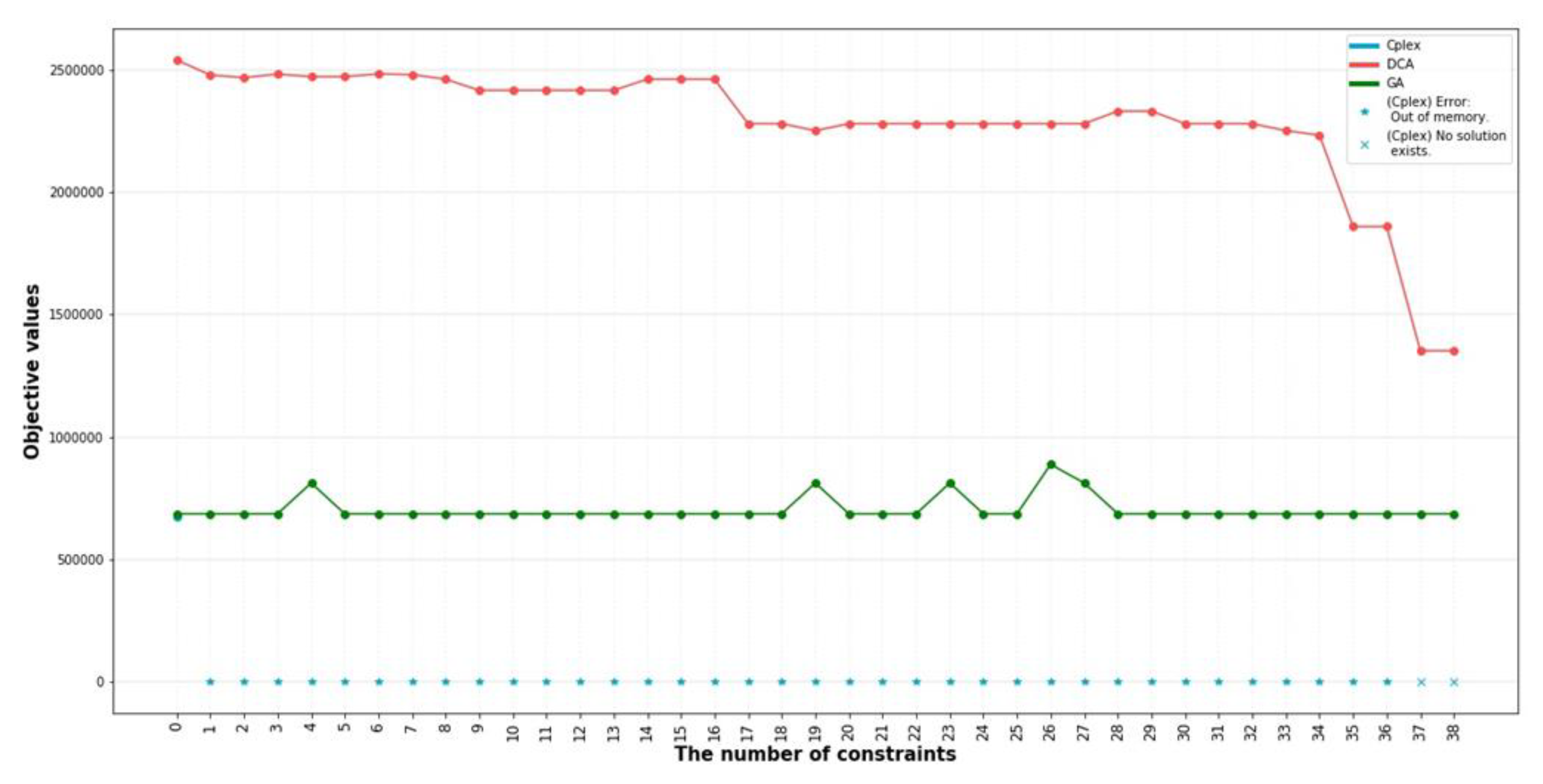
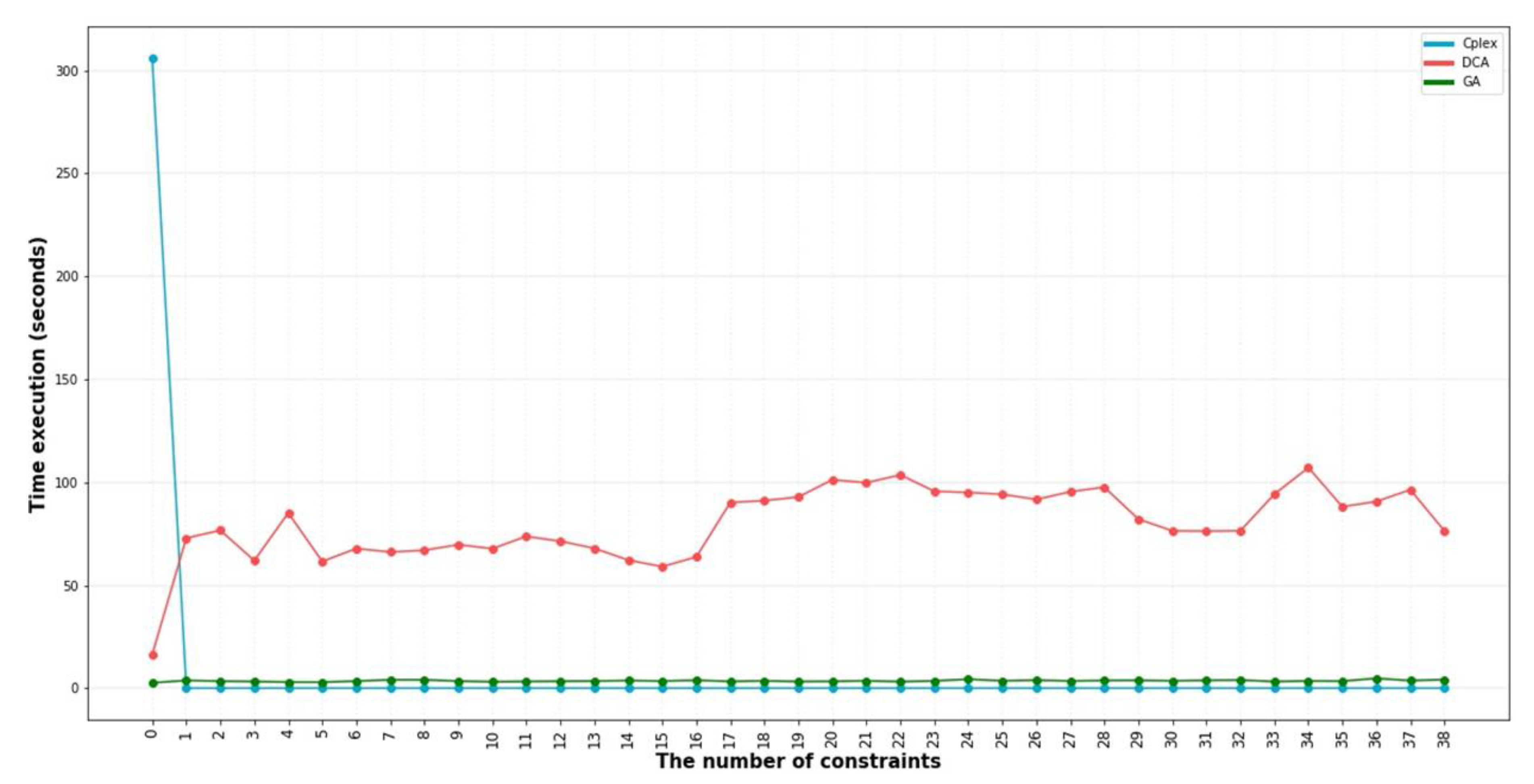
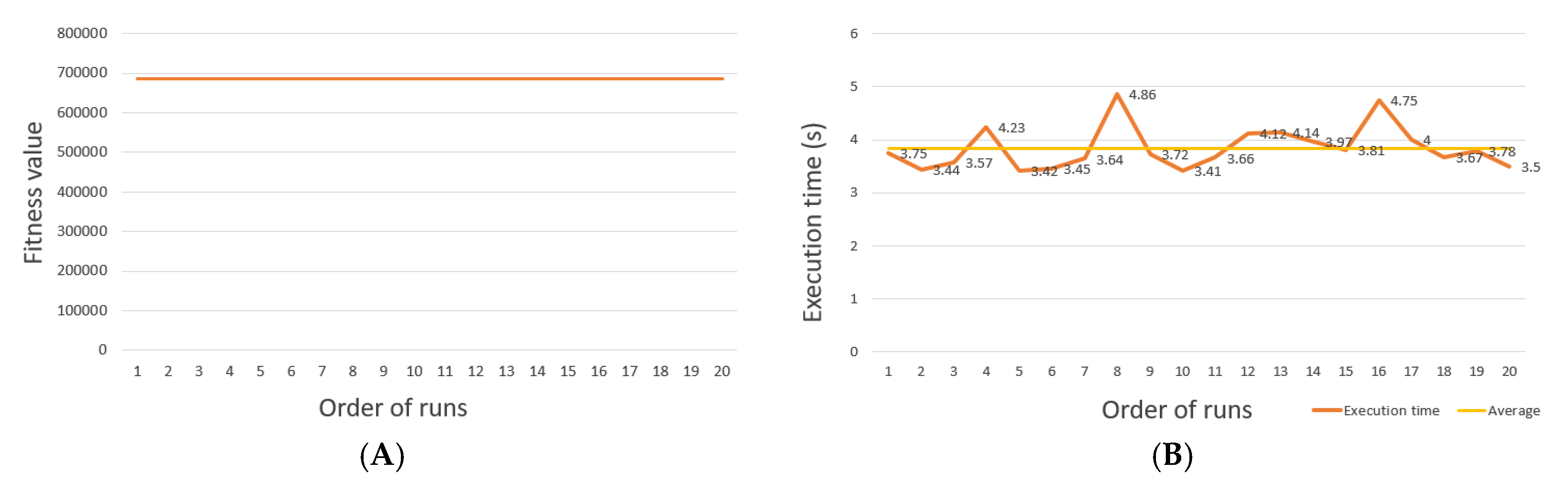
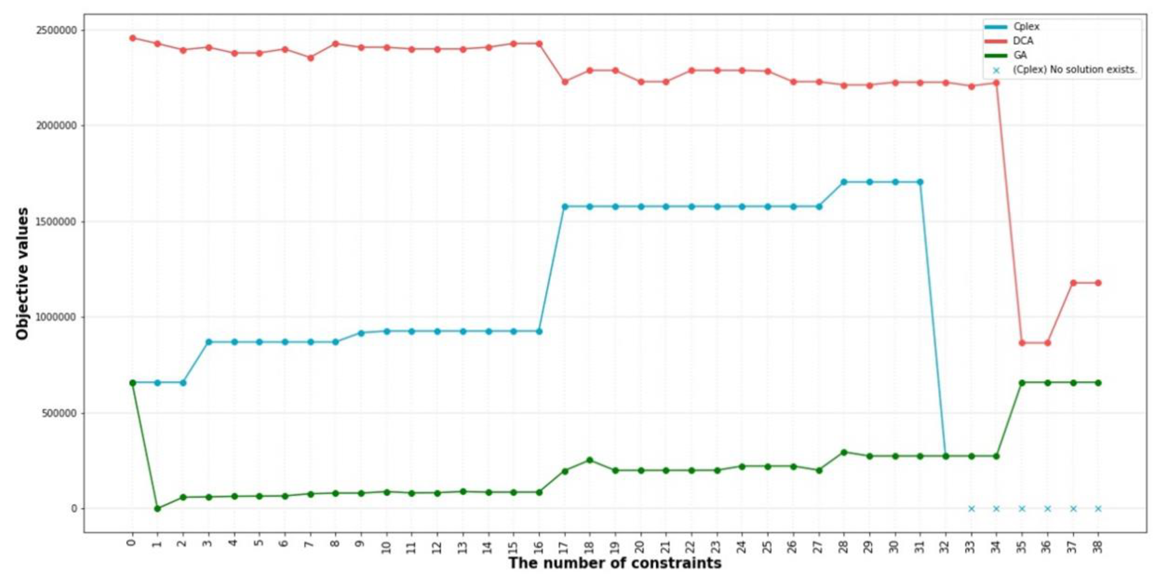
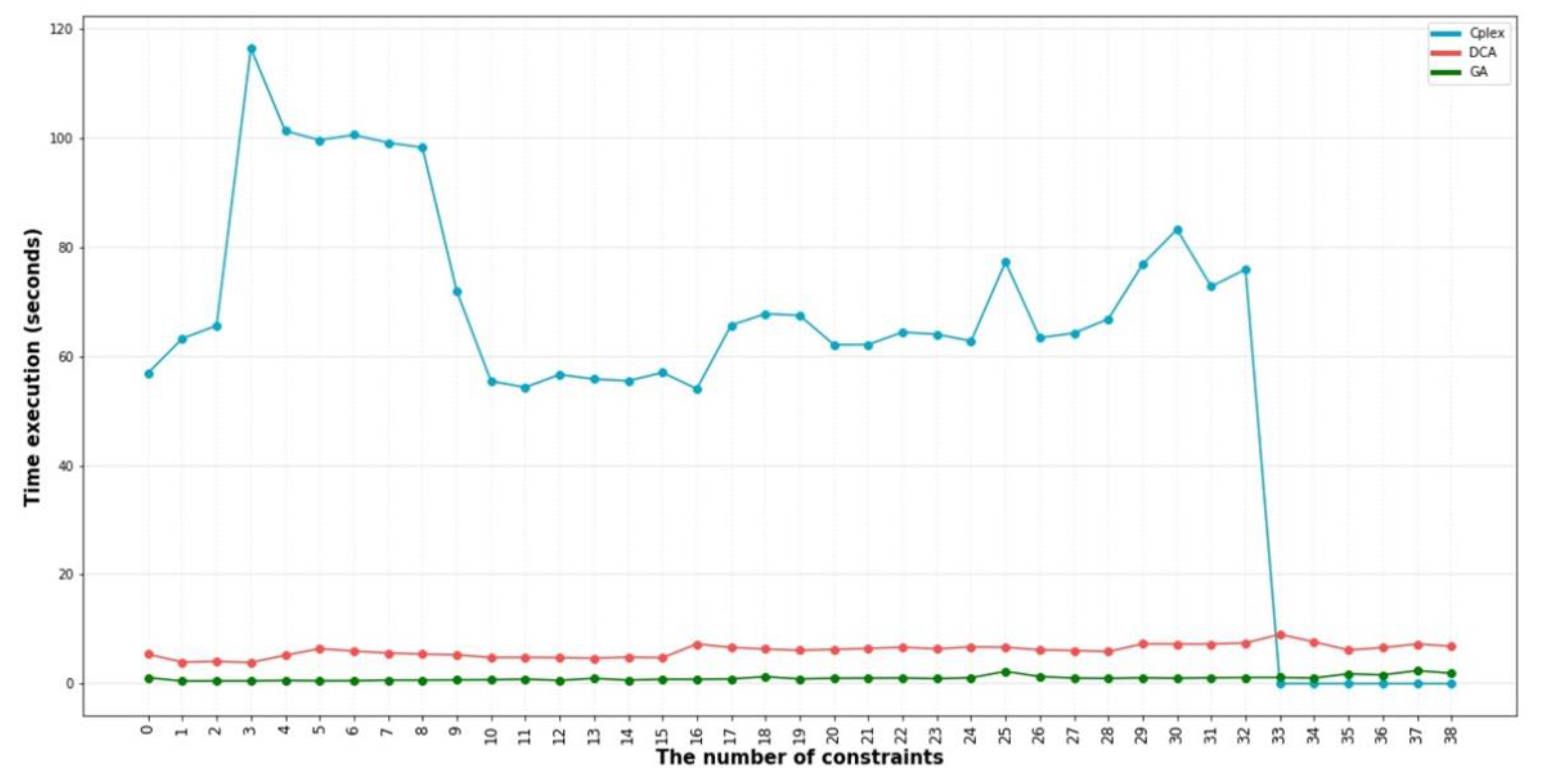
The selected parameters to run the genetic algorithm for further tasks mentioned in

Table 2. Parameter to execute Genetic Algorithm for solving MDSB.

Parameter	G	D	γ	ω	mut	dom	rec
Value	5	0.9	0.1	0.5	0.1	0.6	0.3

.

5.2. Result

We compared DCA, Genetic Algorithm, and CPLEX-MIQP [27] algorithms in terms of the value of objective function and processing time. It is different from the results of the experiment on random generation data with standard distribution and on very little previous experimental data [1,2]. DCA produced excellent results. The above results did not recur in our experiments. After we redesigned another version of the Genetic algorithm, it produced results that outperformed other algorithms. In the first experiment, when we searched for the best team among 3738 contestants. CPLEX only finds the optimal solution in the absence of all business constraints.

The CPLEX and GA found an optimal solution better than the DCA result, but CPLEX needed more time to search. When we add 37 and 38 constraints to the model, CPLEX cannot solve the problem, while other cases have out of memory errors. The results of running all three algorithms to find a team of three members from 3728 candidates displayed in Figure 11 and Figure 12. The new design of the genetic algorithm yielded the best objective value and the most optimal processing time. It is dozens of times faster than DCA. The result of DCA depends a lot on starting points. These points may fall into the valley that does not contain the optimal global solution. Genetic algorithms created mutations of interest very quickly after some generations by the creation of a large population of individuals.

We execute the proposed scheme of the Genetic Algorithm several times with different initial solutions. The objective values and execution times of different execution shown in Figure 13. Twenty times of executions return the same resolution, and the average execution time is about 3.8 s. It shows that the set of selected parameters balanced the two expected factors: execution time and optimum solution.

We conduct a comparison of the algorithms we have designed with CPLEX once again. We realize that CPLEX will consume many resources corresponding to the number of decision variables that it must handle. We, therefore, reduced the remaining set of candidates to 2000—these are the top candidates. Other parameters remain the same. Figure 14 illustrates the returned objective values of the algorithms to find a team of three members from the top 2000 candidates in the dataset. The genetic algorithm not only gives optimal results better than DCA and CPLEX, but also the processing time is much lower. It is ten times faster than DCA and hundreds of times more than CPLEX (see Figure 15). CPLEX can only provide solutions for models with up to 32 business constraints. It is futile for the remaining cases. CPLEX’s long processing time is understandable because it looks for a global solution while DCA and GA look for a local solution.

We see that both DCA and GA algorithms are not committed to finding a universal optimal solution. However, both allow the modeler to make customized designs easily for each specific case. DC helps to transform MDSB to PMDSB with continuous relaxation constraints. This great feature is suited to applying DCA, including addressing a chain of approximate convex programs whose solutions exist. The genetic algorithm creates mutations on a large population. The crossover step helps to deliver best-fitness genes quickly. Finally, an optimal solution is given. It is simple but useful. Both algorithms have shown themselves to be a valuable tool to solve the team selection problem. Although many factors govern the results of both DCA and GA, as mentioned in the previous part, depending on the situation, we can refine the model and parameters to get a solution that Black Box solvers like CPLEX are very hard to do.

In the team selection problem, two factors that increase the size of the search space are the number of candidates, and the size of the selected team (h). Figure 16 shows the execution times and objective value for different values of h. It is easy to see that the Genetic Algorithm has always found better solutions, even though processing time has increased linearly according to the size of the search space. Meanwhile, the processing time of DCA has almost no effect.

6. Conclusions

This study upgraded the team selection model proposed in [1]. A model that helps access both “deep” and “broad” aspects when evaluating teams. We have perfected both the setup and the theoretical gaps. There are some hasty judgments refined in this article. The proposed MDSB model is a compromise model of the bi-objective optimization problem, which helps decision-makers in the decision-making process without having to consider the parameters for each goal. This approach is not only suitable for the ACM team selection problem, but also to the general team selection problem.

The compromise model has made the problem become a MIQP form, although many available solvers are supposed to be able to solve this problem. In our experiment, CPLEX was unable to find the solution when fully binding the business constraint. Instead of using a solver search for the global solution, the proposed heuristic algorithms yield the expected results. In [1], we introduced a rushed implementation of the Genetic Algorithm. However, the current development version has brought a lot of better results. If in [2] the DCA algorithm yielded absolute excellent results, in experiments with actual data, it did not achieve the same effect as cyclic. Although DCA, with many of its useful properties, has proven its effectiveness in many different fields, we have corrected a small mistake of the DCA algorithm and added the convergence proof part of the algorithm.

Even though we have achieved some results, many works remain for future jobs. Both the DCA and the Genetic Algorithm rely heavily on the data, the origin, and design. Therefore, in the future, we will look for ways to improve our settings on the listed aspects. Other meta-heuristics that can resolve the combinatorial optimization problem reviewed in [28] are also promising in order to find useful algorithms. We plan to apply these algorithms to our proposed model shortly. We have not done much when it comes to the shortcomings associated with evaluating the soft skills of candidates. This aspect is also the work we need to do in future research.

References

1. Son, N.T.; Thanh, L.V.; Duong, T.B.; Anh, B.N. A decision support tool for cross-functional team selection: Case study in ACM-ICPC team selection. In Proceedings of the 2018 International Conference on Information Management & Management Science (IMMS ’18), Chengdu, China, 25–27 August 2018; Association for Computing Machinery: New York, NY, USA, 2018; pp. 133–138. [Google Scholar] [CrossRef]
2. Son, N.T.; Thu, T.T.; Anh, B.N.; Dinh, T.V. DCA-Based Algorithm for Cross-Functional Team Selection. In Proceedings of the 2019 8th International Conference on Software and Computer Applications (ICSCA ’19), Penang, Malaysia, 19–22 February 2019; Association for Computing Machinery: New York, NY, USA, 2019; pp. 125–129. [Google Scholar] [CrossRef]
3. Keller, R.T. Cross-functional Project Groups in Research and New Product Development: Diversity, Communication, Job Stress and Outcomes. Acad. Manag. J. 2001, 44, 547–555. [Google Scholar]
4. Parker, G. Cross Functional Teams: Working with Allies, Enemies and Other Strangers; Jossey Bass, A Wiley Imprint: San Francisco, CA, USA, 2003; pp. 4–15. Available online: www.josseybass.com (accessed on 12 November 2019).
5. Wang, Z.; Yan, H.S.; Ma, X.D. A quantitative approach to the organization of cross-functional teams in concurrent engineering. Int. J. Adv. Manuf. Technol. 2003, 21, 879–888. [Google Scholar] [CrossRef]
6. Das, D. Moneyballer: An Integer Optimization Framework for Fantasy Cricket League Selection and Substitution. 2014. Available online: http://debarghyadas.com/files/IPLpaper.pdf (accessed on 12 November 2019).
7. Bhattacharjee, D.; Saikia, H. An objective approach of balanced cricket team selection using binary integer programming method. OPSEARCH 2016, 53, 225–247. [Google Scholar] [CrossRef]
8. Sandhya, S.; Garg, R.; Garg, R. Implementation of multi-criteria decision making approach for the team leader selection in IT sector. J. Proj. Manag. 2016, 1, 67–75. [Google Scholar] [CrossRef]
9. Feng, B.; Jiang, Z.-Z.; Fan, Z.-P.; Fu, N. A method for member selection of cross-functional teams using the individual and collaborative performances. Eur. J. Oper. Res. 2010, 203, 652–661. [Google Scholar] [CrossRef] [Green Version]
10. Fan, Z.-P.; Feng, B.; Jiang, Z.-Z.; Fu, N. A method for member selection of R&D teams using the individual and collaborative information. Expert Syst. Appl. 2009, 36, 8313–8323. [Google Scholar] [CrossRef]
11. Su, J.; Yang, Y.; Zhang, X. A Member Selection Model of Collaboration New Product Development Teams Considering Knowledge and Collaboration. J. Intell. Syst. 2016, 27, 213–229. [Google Scholar] [CrossRef]
12. Van Veldhuizen, D.A.; Lamont, G.B. Multiobjective Evolutionary Algorithms: Analyzing the State-of-the-Art. Evol. Comput. 2000. [Google Scholar] [CrossRef] [PubMed]
13. Hwang, C.-L.; Masud, A.S.M. Multiple Objective Decision Making, Methods and Applications: A State-of-the-Art Survey; Springer: Berlin/Heidelberg, Germany, 1979; ISBN 978-0-387-09111-2. [Google Scholar]
14. Zeleny, M. Compromise Programming. In Multiple Criteria Decision Making; Cochrane, J.L., Zeleny, M., Eds.; University of South Carolina Press: Columbia, SC, USA, 1973; pp. 262–301. [Google Scholar]
15. Edmondson, A.C.; Harvey, J. Cross-boundary teaming for innovation: Integrating research on teams and knowledge in organizations. Hum. Resour. Manag. Rev. 2018, 28, 347–360. [Google Scholar] [CrossRef]
16. Lazimy, R. Mixed-integer quadratic programming. Math. Program. 1982, 22, 332. [Google Scholar] [CrossRef]
17. Le Thi, H.A.; Pham Dinh, T. DC programming and DCA: Thirty years of developments. Math. Program. 2018, 169, 5–68. [Google Scholar] [CrossRef]
18. Duy, N.T.; Thuy, T.T.; Chung, L.T.; Son, N.T.; Dinh, T.V. DC programming and DCA for Secure Guarantee with Null Space Beamforming in Two-Way Relay Networks. In Proceedings of the 2019 8th International Conference on Software and Computer Applications (ICSCA’19), Penang, Malaysia, 19–21 February 2019; ACM: New York, NY, USA, 2019; pp. 529–532. [Google Scholar] [CrossRef]
19. Thuy, T.T.; Nam, N.V.; Son, N.T.; Dinh, T.V. DC Programming and DCA for Power Minimization Problem in Multi-User Beamforming Networks. In Proceedings of the 2019 8th International Conference on Software and Computer Applications (ICSCA’19), Penang, Malaysia, 19–21 February 2019; ACM: New York, NY, USA, 2019; pp. 564–568. [Google Scholar] [CrossRef]
20. Phan, D.N.; le Thi, H.A. Group variable selection via lp,0 regularization and application to optimal scoring. Neural Netw. 2019, 118, 220–234. [Google Scholar] [CrossRef] [PubMed]
21. Le Thi, H.A.; Ho, V.T. Online Learning based on Online DCA and Application to Online Classification. Neural Comput. 2020, 32, 1–35. [Google Scholar] [CrossRef] [PubMed]
22. An, L.T.H.; Tao, P.D.; Muu, L.D. Exact Penalty in D.C. Programming. Vietnam J. Math. 1999, 27, 169–178. [Google Scholar]
23. Thede, S.M. An Introduction to Genetic Algorithms. J. Comput. Sci. Coll. 2004, 20, 115–123. [Google Scholar]
24. Sharp, G.D.; Brettenny, W.J.; Gonsalves, J.W.; Lourens, M.; Stretch, R.A. Article: Integer optimisation for the selection of a Twenty 20 cricket team. J. Oper. Res. Soc. 2011, 62, 1688–1694. [Google Scholar] [CrossRef]
25. Burney, A.S.M.; Mahmood, N.; Rizwan, K.; Amjad, U. Article: A Generic Approach for Team Selection in Multi-player Games using Genetic Algorithm. Int. J. Comput. Appl. 2012, 40, 11–17. [Google Scholar]
26. Codeforce API. Available online: https://codeforces.com/apiHelp (accessed on 2 February 2020).
27. IBM ILOG CPLEX Optimization Studio. CPLEX User’s Manual. Version 12 Release 8. Available online: https://www.ibm.com/support/knowledgecenter/SSSA5P_12.7.0/ilog.odms.studio.help/pdf/usrcplex.pdf (accessed on 2 February 2020).
28. Muthuraman, S.; Venkatesan, V.P. A Comprehensive Study on Hybrid Meta-Heuristic Approaches Used for Solving Combinatorial Optimization Problems. In Proceedings of the 2017 World Congress on Computing and Communication Technologies (WCCCT), Tiruchirappalli, India, 2–4 February 2017. [Google Scholar]
Figure 1. Illustration of the team selection problem. The table at the left of the figure describes the aggregated data through the competitions and training of the candidates. The goal is to select the team with the highest potential for achievement.
Applsci 10 02700 g001
Figure 2. Basic workflow of the genetic algorithm.
Applsci 10 02700 g002
Figure 3. The number of users of codeforces.com in Southeast Asian countries.
Applsci 10 02700 g003
Figure 4. The scores of 8 skills of the top 10 users in Vietnam.
Applsci 10 02700 g004
Figure 5. The total number of scores the user has achieved by solving exercises for each skill.
Applsci 10 02700 g005
Figure 6. The minimum, maximum, and average scores that the users gained for their skills.
Applsci 10 02700 g006
Figure 7. Probability density graphs on corresponding skills: (A) math, implementation, brute force, dp, greedy; (B) binary search, sortings, constructive algorithms, data structures, strings; (C) geometry, bitmasks, trees, combinatorics, two pointers; (D) divide and conquer, games, shortest paths, hashing; (E) meet-in-the-middle, graph matchings, expression parsing, schedules; (F) number theory, dfs and similar, graphs; (G) *special; (H) probabilities, interactive, dsu; (I) matrices, flows, string suffix structures, ternary search; (J) Chinese remainder theorem, fft, 2-sat.
Applsci 10 02700 g007aApplsci 10 02700 g007b
Figure 8. The procedure of the experiment.
Applsci 10 02700 g008
Figure 9. (A) the time execution of DCA with different values of τ; (B) the objective value of DCA with different values of τ; (C) average errors of the decision variables with different values of τ.
Applsci 10 02700 g009
Figure 10. (A) the fitness values over generations; (B) the execution times over generations.
Applsci 10 02700 g010
Figure 11. The objective value of three tested algorithms to find a team of three members from 3728 candidates.
Applsci 10 02700 g011
Figure 12. The time execution of three tested algorithms to find a team of three members from 3728 candidates.
Applsci 10 02700 g012
Figure 13. (A) the objective values of genetic algorithm corresponding to different initial points. (B) the execution times of genetic algorithm corresponding to different initial points.
Applsci 10 02700 g013
Figure 14. The objective values of the algorithms to find a team of three members from the top 2000 candidates.
Applsci 10 02700 g014
Figure 15. The time execution of the algorithms to find a team of three members from the top 2000 candidates.
Applsci 10 02700 g015
Figure 16. (A) the objective values of the algorithms with different team size; (B) the execution time of the algorithms with different team size.
Applsci 10 02700 g016