Numerical and Experimental Study on the Flow-Induced Noise Characteristics of High-Speed Centrifugal Pumps

Abstract

The development of low-noise pumps is essential to design quiet fluid delivery systems. Due to the complicated internal flow, the flow-induced noise characteristics of high-speed centrifugal pumps have not been well understood. Taking engine cooling pumps as an example model, experimental measurements are performed in a semi-anechoic room and a CFD/CFA calculation method is proposed to study the fluid-borne noise and radiated noise characteristics. In the speed range of 5000–6750 r/min, both the pump head and the dimensionless radiated noise characteristics conform to similar laws, and the highest efficiency point pump presents the lowest noise level. Consistent with the experimental results, the predicted radiated noise of the model pump presents dipole characteristics at the required flow rate condition. Moreover, the spectrum of fluid borne noise at pump outlet shows broadband characteristics but with obvious discrete peaks, which are not only related to the fluid pressure pulsation characteristics (6f₀ and the multiple) at the low-frequency region, but also to the frequency of the structural mode (3000–6000 Hz region). Rotor-stator interaction of the pump flow field between the impeller and volute is the main reason of flow-induced noise; unstable flow also contributes to the broadband components in the noise spectrum.

1. Introduction

Pumps are widely used in social and economic life, such as high building water supply, engine cooling, chemical process, nuclear power, and so on, most of which are centrifugal pumps. With the same head requirements, lifting the rotational speed of the impeller can reduce the size of the pump. Therefore, developing high-speed centrifugal pumps is one of the development trends in this engineering application area [1,2]. However, it will also bring serious vibration and noise problems with a detrimental impact on the environment. According to the mechanism of sound production, the noise may arise from mechanical vibrations or from the unsteady flow of the working fluid, namely, flow-induced noise [3,4]. Consequently, mechanical quieting techniques experienced great advances in recent years. These techniques had little effect, however, on reducing hydraulic noise transmitted through water. In particular, the internal flow of the high-speed centrifugal pump is more complicated. So, fluid-generated noise in pumps has become a subject of much greater interest in recent years.

Due to the demand from the user for silent fluid transporting systems, the flow-induced noise mechanism has received more and more attention from the researchers. In 1952, Lighthill [5] solved the problem of the jet noise generated aerodynamically by an engine under the free space assumption by using an acoustic analogy, which is marked as the birth of aeroacoustics or flow-induced noise. Through the continuous efforts of later research, the Lighthill acoustic analogy equation has been further extended to understand the generation and propagation of flow-induced noise [6]. Meanwhile, research on pump noise is also underway. Simpson et al. [7] examined two types of centrifugal pumps—volute pumps and diffuser pumps—to determine the effect of design and operating conditions on the level of noise generated in the pumped liquid. Chu et al. [8,9] made a particle displacement velocimetry (PDV) experiment together with noise and local pressure measures on a laboratory centrifugal pump and found that blade–tongue interactions and non-uniform outflow from the impeller are primary contributors to local pressure fluctuations and far-field noise. Choi et al. [10] reported on an experimental investigation of large-scale flow field instabilities in a pump rotor, where the measured jet-wake type of instability flow causes a periodic pressure fluctuation on the blade surface and generates noise. Černetič [11] used noise signals to detect the inception and development of a cavitation phenomenon in the pump. With the development of aeroacoustics and computational fluid dynamics (CFD), the numerical method has become an important analysis method for flow-induced noise. Langthjem and Olhoff [12] developed a method to predict flow-induced noise by reputing unsteady impeller blade surface forces as rotating diploe and applied it in a two-dimensional centrifugal pump. Parrondo et al. [13] presented a simple acoustic model for centrifugal pumps that considers ideal sound sources of arbitrary position and properties, concluded that the sound field can be characterized reasonably by a dipole-like source located at the tongue region. Keller et al. [14] obtained the influence of different acoustic impedances of the suction side on the pressure fluctuations at the pump by using the matrix formulation acoustic model. Mao et al. [15] combined the detached eddy simulation (DES) method and the acoustic boundary element method involved in software LMS to predict the flow-induced noise characterization of pump turbines during a transient load rejection process and intermittent vane closing conditions. The above research mainly focuses on fluid borne noise and dipole source around volute cut-off. Jiang et al. [16] used LES-based CFD program to simulate the interior flow field of a five-stage centrifugal pump, developed a data-interface tool to solve the problem of data exchange between fluid and structural grids, and proved it is feasible to use fluid–structure weakly coupled simulations to estimate the flow-induced noise generated in turbomachinery. Si et al. [17,18] proposed a numerical calculation method of flow-induced noise in a centrifugal pump combining CFD and CA (computational acoustics). It can be used to calculate the radiated noise after considering the vibro-acoustic effect of pump casing, which are applied on radiated noise prediction of a multi-stage pump under different flow rates and a washing machine pump under two-phase flow. Kapellos et al. [19] developed the unsteady continuous adjoint method by using an incompressible improved delayed DES and the acoustic Kirchhoff integral method to predict the flow-induced sound radiation from a body in free-stream. The flow-induced noise prediction is also a very attractive theme in other turbo machinery such as fans and blowers. Velarde and Tajadura [20] numerically studied the tonal noise of a centrifugal fan by solving the Powell wave equation. Powell’s theory of votex sound has an advantage in explaining the mechanism of flow-induced noise, which expresses noise generation as a function of velocity and vorticity fields. Cravero and Marsano [21] developed a CFD procedure to accurately predict the tonal noise in radial bowers. Accurate flow noise prediction based on analogy theory is the development trend, but numerical methods that consider both fluid-borne noise and radiated noise still need development at present.

In this paper, a CFD/CFA (computational fluid dynamics/computational fluid acoustic) method is proposed to calculate the fluid-borne noise and flow-induced radiated noise of high-speed centrifugal pumps based on Lighthill’s acoustic analogy theory. A test rig was set up in the semi-anechoic room to give the initial boundary conditions and verify the calculation results. The pump performance and sound pressure levels of different speeds are measured. Moreover, the noise spectrum characteristics and directivity characteristics under different working conditions are also obtained. The numerical flow-induced noise characteristics of the high-speed centrifugal pumps under the required working conditions are studied then.

2. Research Object and Methods

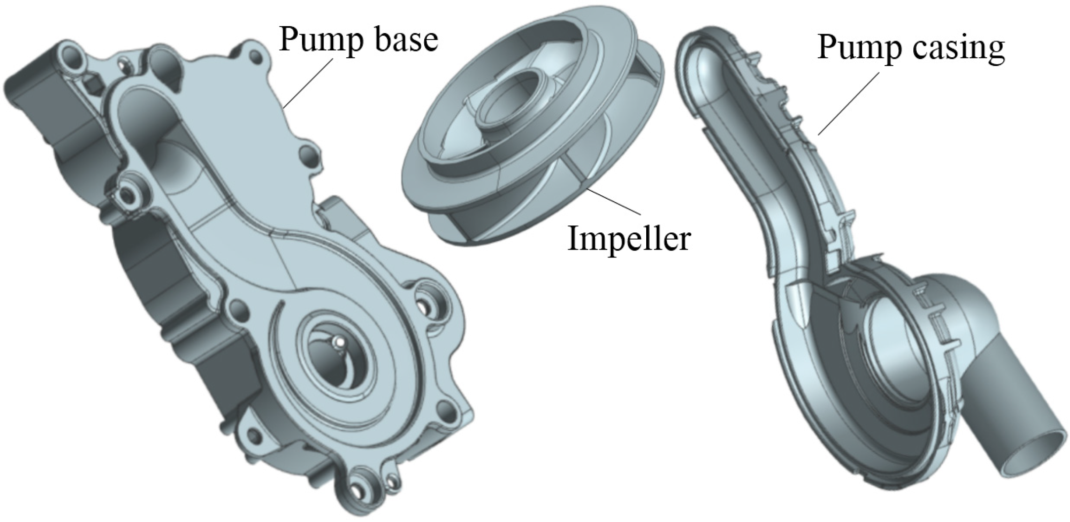
2.1. Pump Model

An engine cooling pump with high rotational speed was selected as the research model. It is the main component to transport the cooling water in the closed-cycle cooling system of automobile engines. The pump performance not only affects the power and economy of the car but also affects the lifetime of the engine. The high-speed engine cooling pumps are always centrifugal ones and coupled with the engine. The impeller is driven by the engine crankshaft through a belt connection, and the flow rate of the delivery cooling fluid is varied according to the engine speed. The structure of this pump model is shown in Figure 1, including pump casing, centrifugal impeller, and pump base. Due to the limitation of space arrangement, the shape of the flow-path structure is complex and the hydrodynamic stability is prominent, which easily leads to serious induced vibration and noise problems destroying the stable operation of the cooling system. Therefore, it is of great significance to study the flow-induced noise characteristics of it to restrict the reliable and quiet working of the system. The operational parameters of the pump at rotational speed n = 6750 rpm are as follows: volume flow rate Q_r = 10.2 m³/h, head H_r = 14 m. The pump impeller has 6 blades, with a diameter of 0.063 m.

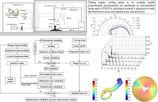
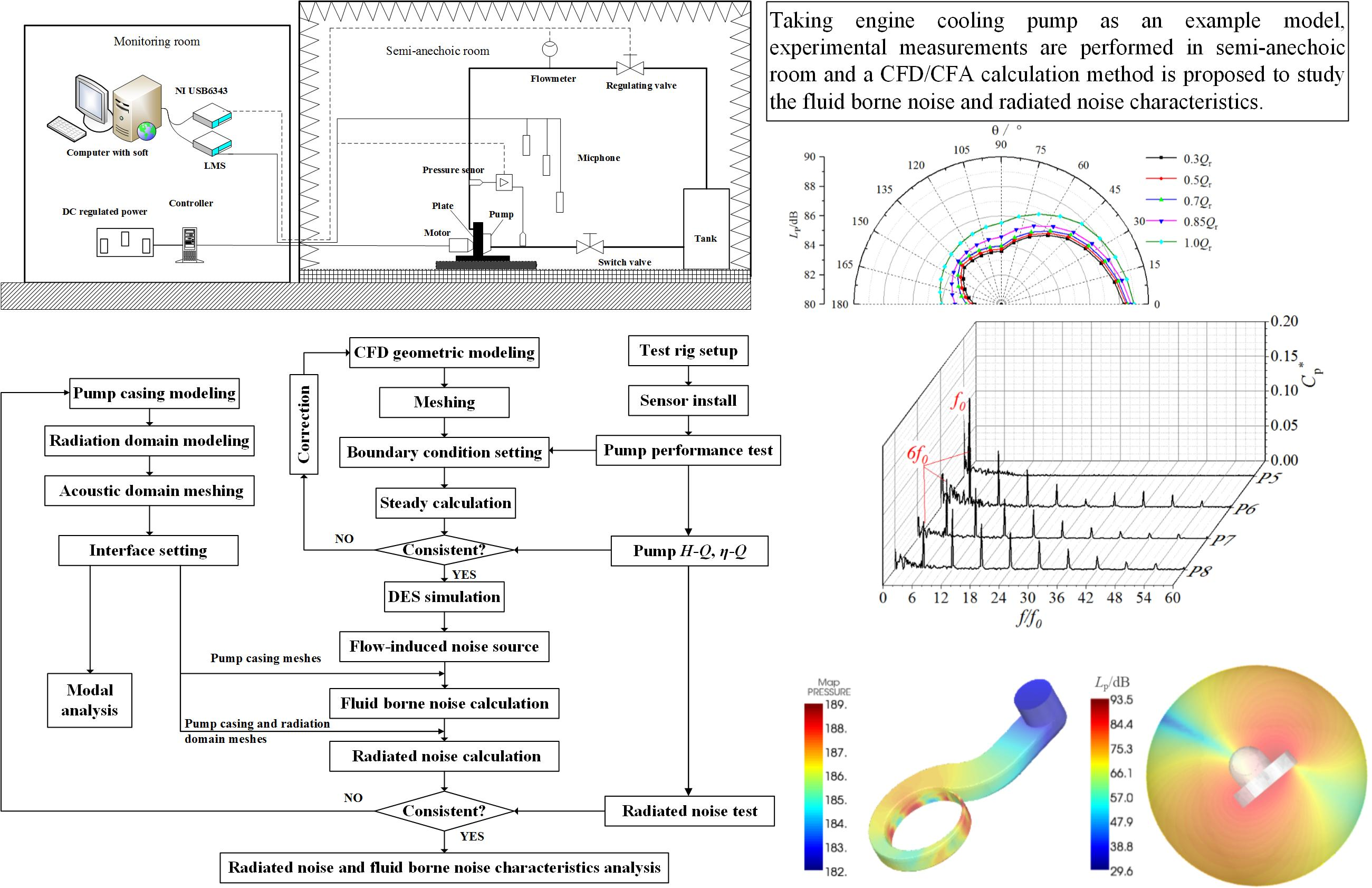
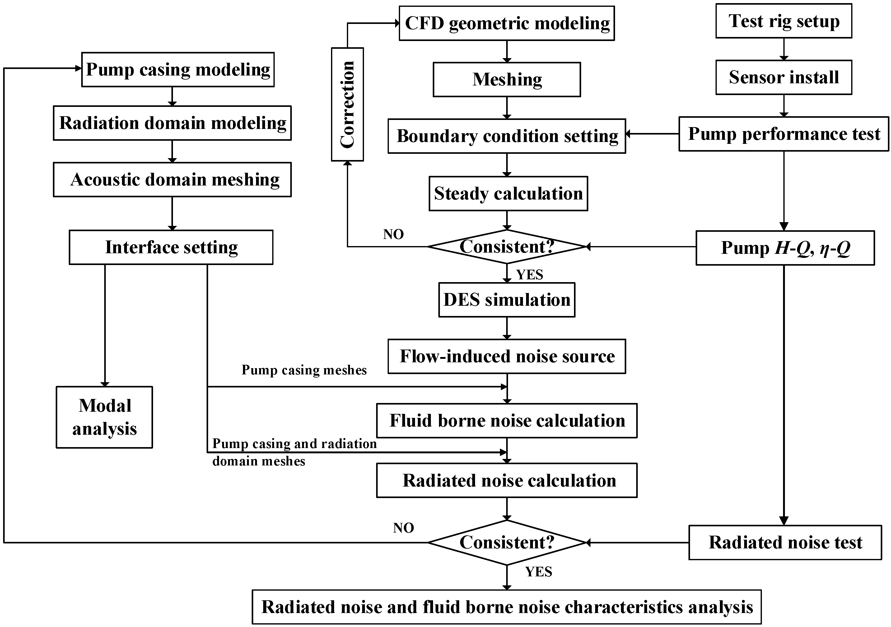
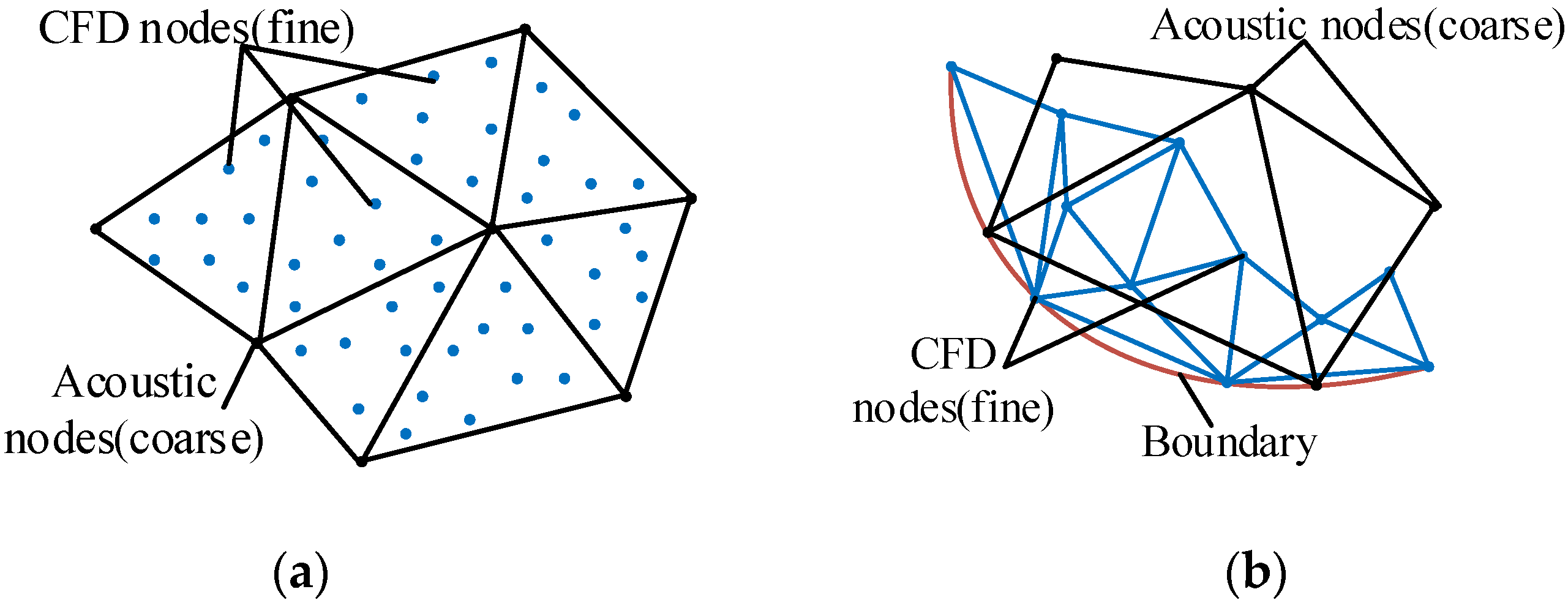
2.2. Theory of the Proposed CFD/CFA

Reasonable numerical simulation methods can make up for the shortcomings of experiments and assist theoretical analysis in revealing the nature of physical phenomena. The proposed experiment-assisted CFD/CFA method in this paper is based on the Lighthill acoustic analogy theory.

Both hydrodynamics and hydroacoustic of the flow field are governed by the compressible Navier–Stokes equations. A direct numerical simulation (DNS) of these equations is impractical on most engineering problems, which calls for an alternative approach. One alternative consists of using an acoustic analogy, as first proposed by Lighthill in the following form [22]:

$$\begin{array}{l}\frac{{\partial }^2}{\partial t^2}\left(\rho -{\rho }_0\right)-c_0{}^2\frac{{\partial }^2}{\partial x_i\partial x_j}\left(\rho -{\rho }_0\right)=\frac{{\partial }^2{T}_{ij}}{\partial x_i\partial x_j}\\ T_{ij}=\rho v_i{v}_j+{\delta }_{ij}[(p-p_0)-c_0{}^2(\rho -{\rho }_0)]-{\tau }_{ij}\end{array}$$

(1)

where ρ represents the density of the fluid, ρ₀ denotes density at rest, v is velocity, p is pressure, T denotes the Lighthill’s tensor, c₀ is the speed of sound at rest, and τ is the viscous stress tensor. In practice, an acoustic analogy uses a two-step procedure. In the first step, an unsteady flow analysis is used to compute hydrodynamics sources. The second step consists in computing the propagation and radiation of the fluid noise sources. The implementation of the second step can be achieved by using frequency-domain formulation. Harmonic perturbations are considered in such a way that any perturbed quantity p can be written as

$$p(x,t)=Re(\tilde{p}(x)e^{iwt})$$

(2)

Away from the source region, the density fluctuations, ρ–ρ₀, correspond to acoustic density fluctuations ρ_c. Then, Lighthill’s equation can be rewritten using the frequency domain transform.

$$\frac{{\partial }^2{\tilde{\rho }}_c}{\partial x_i\partial x_i}+k^2{\tilde{\rho }}_c=-\frac{1}{c_0}\frac{{\partial }^2{\tilde{T}}_{ij}}{\partial x_i\partial x_j}$$

(3)

where k = ω/c₀ denotes the acoustic wavenumber. Equivalently, Lighthill’s analogy in a frequency domain computation requires the Fourier transform of T in the source term, which means every frequency component of T is a function of all frequency components of v. The weak variational statement as follows.

$${\displaystyle \underset{\mathsf{\Omega }}{\int }(k^2}{\tilde{\rho }}_c\delta \rho -\frac{\partial {\tilde{\rho }}_c}{\partial x_i}\frac{\partial \delta \rho }{\partial x_i}-\frac{1}{c_0^2}\frac{\partial {\tilde{T}}_{ij}}{\partial x_j}\frac{\partial \delta \rho }{\partial x_i})dx=0$$

(4)

In general, CFD simulation is used to compute T instead of direct acoustic calculation because of using the finite volume method, which differs from FEM about the way to compute derivatives. Moreover, the CFD mesh is usually finer than the acoustic mesh, which leads to a better approximation of derivatives $\partial {\tilde{T}}_{ij}/\partial x_j$. Through interpolation, the frequency domain sound source information is transferred to the acoustic grid, and the second step of the acoustic calculation is performed using the finite element/infinite element method in the present work.

The flow chart of the computational process is shown in Figure 2. The proposed CFD/CFA method consists of three parts, namely, flow field solving, structure domain solving, and experimental supporting. Firstly, the computational flow domain and corresponding meshes were prepared to process the steady simulation. Simultaneously, the test rig was built to simulate the condition of the engine-cooling system and give out the inlet and outlet boundary conditions for the CFD. The obtained pump performance data, such as the pump head and efficiency, are used to verify or modify the appropriate grid and the numerical calculation model. The SST (shear stress transport) model embedded in ANSYS CFX 14.1 software (ANSYS, Inc., Commonwealth of Pennsylvania, USA) was repeatedly used at this step. Secondly, the unsteady simulation based on the DES method is processed to calculate the flow field of the model pump. Afterwards, detailed flow information, such as flow velocity, pressure, and density, are extracted and transformed as the sound source for the next acoustic simulation. Considering that the flow pattern inside the high-speed centrifugal pump is complex and the acoustic simulation domain is irregular, the FEM (finite element method) is further used in the fluid borne noise simulation, which could well transform the sound source. The infinite element method, combined with the above finite element method, is used to calculate the radiated noise field of the model pump. Meanwhile, the fluid acoustic calculation domains and radiate acoustic calculation domains are built along with the acoustic mesh generation containing the interface setting. Finally, the fluid-borne noise and radiated noise calculation are processed using Actran12.0 software (Free Field Technologies MSC Software Company, Mont-Saint-Guibert, Belgium). The one-way numerical coupling method is used when referring to structure vibro-acoustics, which means noise-induced vibrations are ignored in this simulation. The acoustic characteristics of the model pump, such as sound pressure level and frequency domain response, are analyzed after experimental verification.

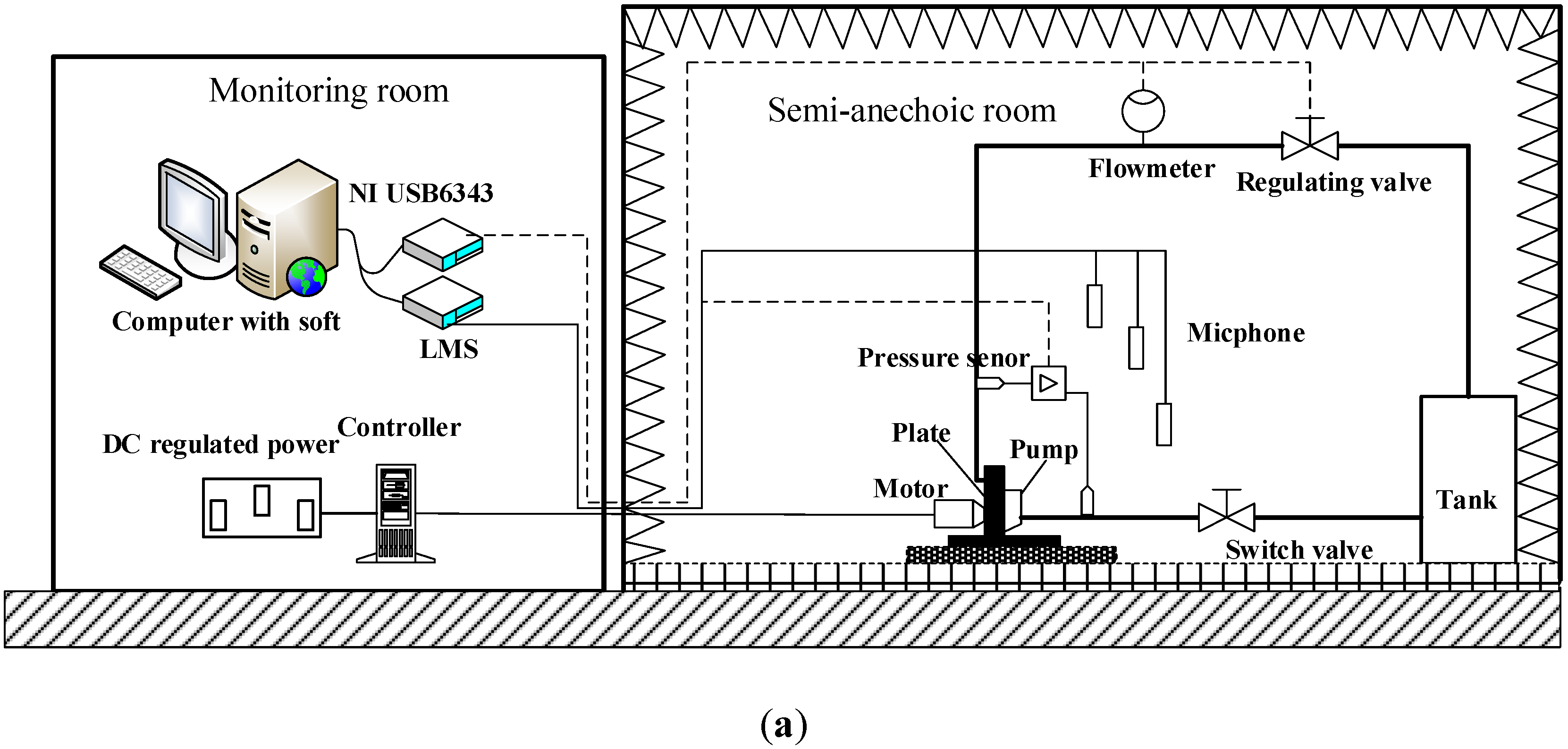
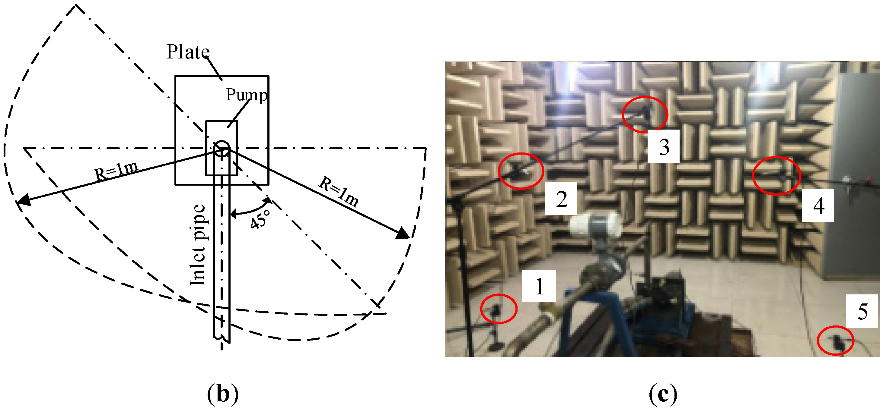
2.3. Experimental Support

The experimental test rig of high-speed centrifugal pumps is built in a semi-anechoic room, as shown in Figure 3a. The open-type system is used to simulate the actual working condition of the cooling water pump. A tank, together with the valves, adjusts the resistance of the circulation system and the pump inlet pressure. In order to reduce the noise interference during the measurement, the experiment uses a motor to drive the pump instead of the engine drive. The pump base is welded on the thick iron plate, and the pump shaft is connected to a permanent magnet DC motor. In this pipeline system, all parts are wrapped with sound-absorbing cotton. The stabilized voltage supply and all the data collection equipment is put in the monitoring room to improve the accuracy of the measurement. The semi-anechoic room supplies a damping base to install the pump loop with 15 dB background noise and 50 Hz cut-off frequency measurement surroundings. The test system includes a pump performance measurement module and a noise data collection module. The flow rate is obtained by an LDCK-32JM25MY/TBS type electromagnetic flowmeter with a range of 0–45 m³/h. The head of the pump, defined by Equation (1), is measured by a CYG1204F type differential pressure transducer with a range of 0–300 kPa. The data acquisition system consists of an NI6343 data acquisition card and the LabVIEW acquisition program. Typically, the main parameters used to evaluate pump performance are head and efficiency. The head represents the ability of the centrifugal pump to transport water, usually expressed as the height of the water H. It can be expressed as the increase in the pressure energy, kinetic velocity energy, and potential energy of the fluid, defined by Equation (5). The efficiency of centrifugal pumps is the ratio of useful power to input power, defined in Equation (6).

$$H=\frac{p_2-p_1}{\rho g}+\frac{v_2{}^2-v_1{}^2}{2g}+\left(z_2-z_1\right)$$

(5)

$$\eta =\frac{\rho gQH}{P_e}$$

(6)

where p₁ and p₂ imply the inlet pressure and outlet pressure, respectively; v₁, v₂ denote the average velocities of the inlet and outlet section, respectively; z₁, z₂ are the heights at the inlet and outlet center section of the model pump to the reference horizontal plane; ρ denotes the fluid density; g denotes the standard acceleration of gravity; P_e is the shaft power calculated by the input power and motor efficiency. The accuracy of the flow rate measurements is 0.5%; the rotational speed uncertainty is 1%. The estimated uncertainty of head measurement is below 0.32%, and efficiency uncertainty is no more than 0.72%, which meets the Grade 1 accuracy based on the ISO 9906.2012 standard [23].

The noise is measured with the PCB 14043 type microphone (PCB Piezotronics Inc., New York, USA) and processed based on the LMS Test Lab platform. The accuracy of the SPL of the radiated noise is ±1 dB. The acquisition sampling frequency is set to 6400 Hz, and the resolution frequency is set to 1 Hz. Every test used 120 s for the signal acquisition and treated frequency resolution by the Hanning window in general. Five microphones set to evaluate noise level and sound source directivity followed the Chinese standard GB/T 29529-2013 [24]. The position of the microphone sensor is as shown in Figure 3b, all the microphone sensors are uniformly distributed as a semicircle with a distance of 1 m to the high-speed centrifugal pump. In order to accurately capture the intensity distribution of the radiated noise field, two sets of microphone sensors are arranged, respectively, in the direction perpendicular to the inlet tube and 45 °oblique to the inlet tube. The average total sound pressure level L_P is expressed as Equation (3) in order to analyze the variation of the radiated noise levels. N represents the number of sound monitoring points, and L_pi is the total sound pressure level of each sound monitoring point. P_ref is the reference sound pressure, which is equal to 2×10^-5 Pa.

$$\begin{array}{l}{L}_p=20\lg (P_e/P_{ref})\\ {\overline{L}}_P=10\cdot \lg \left[\frac{1}{N}{\displaystyle \sum _{i=1}^N{10}^{0.1L_{Pi}}}\right]\end{array}$$

(7)

2.4. Numerical Setups

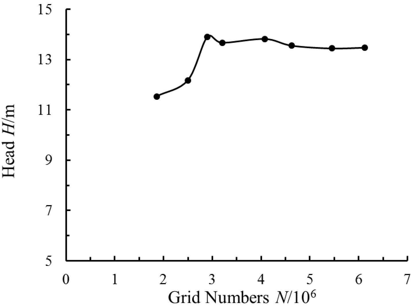
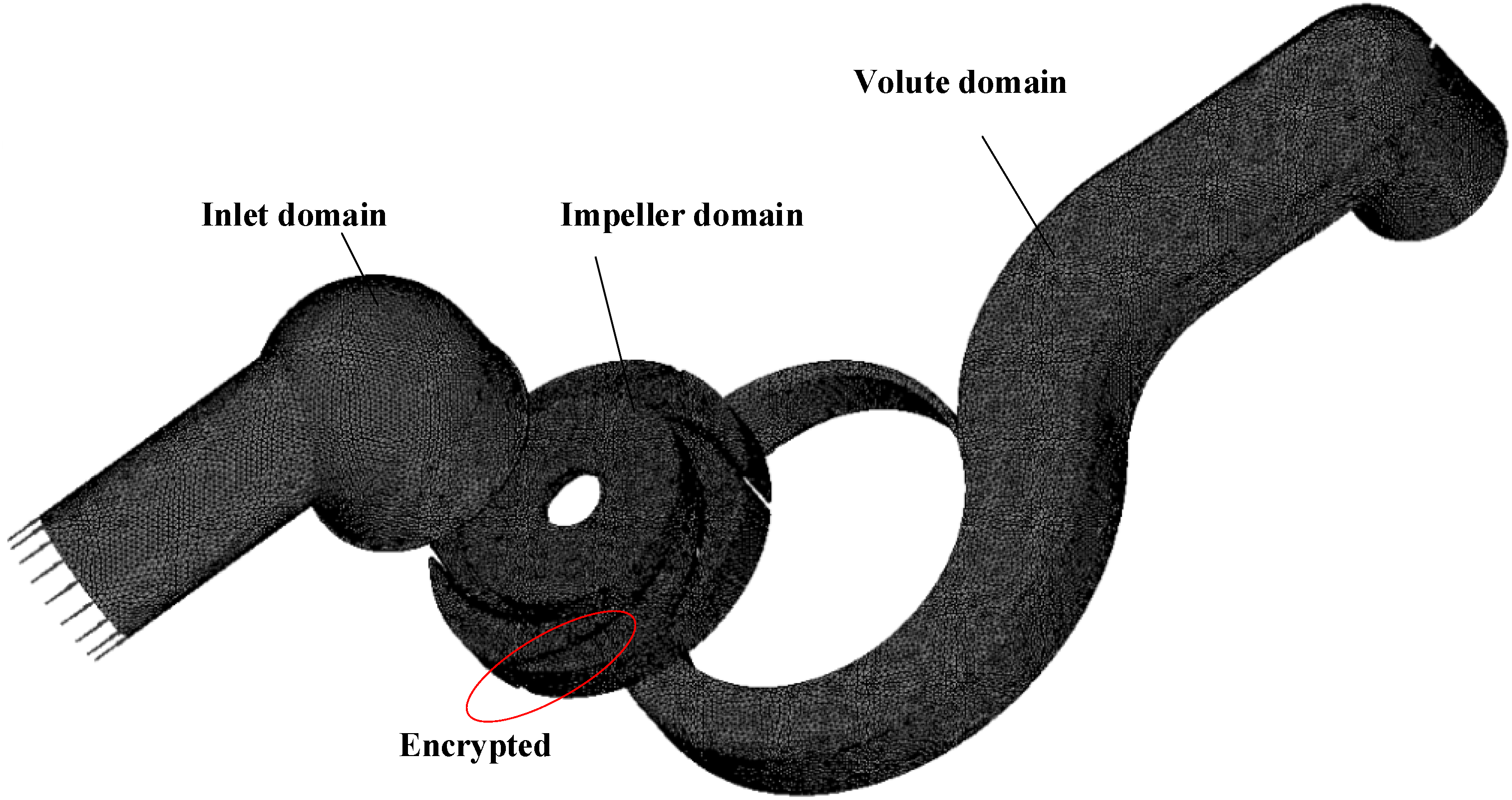
2.4.1. Computation Domain and Mesh Generation of the Flow Field

Corresponding to the structure diagram shown in Figure 1, the computing domain of the high-speed pump flow field is also divided into four parts, namely, inlet domain, impeller domain, volute domain, and outlet pipe domain. The influence of both sealing and structural chamfering is ignored in order to improve the simulation efficiency. Combined with the actual inflow situation, the inlet and outlet pipe domain are extended appropriately to reduce the influence of backflow boundary conditions [25].

Professional mesh generation software ANSYS ICEM 14.1 is used to perform meshing of the computational domains. Due to the irregularity of the flow channel volume, unstructured mesh technology is used to divide the grid, the same as subsequent acoustic mesh generation. In order to eliminate the influence of the number of cells on the accuracy of numerical simulation, the grid independence analysis of head is carried out, the results of which are shown in Figure 4. It can be seen from the figure that when the number of cells is more than 3.18 million, the influence of the increase of the grid number on the head can be ignored. Moreover, places such as the blade wall surface is mesh-encrypted; the final mesh quality of all domains exceeds 0.35. The maximum nondimensional wall distance, 𝑦 + < 60, was obtained in the complete flow field, which means it could satisfy the requirement of all turbulence modeling methods used in this paper. So, meshes with the determined number of 3.18 million cells (as shown in Figure 5) are used for subsequent calculation.

2.4.2. Boundary Conditions and Turbulence Model of the CFD

The inlet and outlet boundary conditions are set according to the values obtained by experiments. In order to obtain a robust calculation, the inlet boundary condition is set to total pressure, and the outlet boundary condition is set to mass flow rate. All the other walls are treated as non-slip boundaries. The pre-converged steady flow field (based on the SST turbulence model) obtained is accepted as the initial condition followed by the unsteady simulation.

In order to acquire accurate acoustic sources, a turbulence model is usually adopted to characterize the unresolved turbulence scales. The Reynolds-averaged Navier–Stokes (RANS) equation is widely used due to the drastic reduction of computational cost for engineering applications on predicting the flow details. However, it only resolves the time-averaged flow-lacking of frequency-related term, which makes it inappropriate for flow-induced acoustics. LES resolves the large eddies and implicitly accounts for the small eddies by using a sub-grid scale model, which is a mainstream turbulence model for simulating the acoustic problems in a fluctuating flow field. The flow field of a high-speed centrifugal pump may exhibit phenomena such as backflow, flow separation, inlet distortion, and rotator–stator interaction, as well as mutual interferences. A sub-grid scale model is used to equalize the flow variables as instantaneous values within the spatial domain, through which the pressure fluctuating phenomenon can be captured from the separated flow. At present, it is impossible to simulate the small-scale eddy due to the wall separation with coarse meshes. Moreover, a near-wall model cannot soundly simulate the near-wall flow structures and the growth-separation phenomena of boundary layers unless it uses micro-sized grids. So far, the computational cost for solving such an engineering problem by using LES is mostly beyond the available computational capabilities. The unsteady RANS model makes it possible to calculate the flow fluctuation by adding an additional time term to the RANS equations. A hybrid method to combine the advantages of LES and RANS models has been popularly developed. SAS is a hybrid turbulence model that introduces the von Karman length scale based on the URANS model. It can dynamically adjust the length scale and does not need to divide the computational domain into the URANS and LES computing regions through the grid-scale, which allows simulating fluctuating flow using a large-eddy model. However, this model may be unstable in solving weak high-wave number dissipation problems, where instability is caused by the mesh when it is not capable of producing small-scale eddies small-scale eddy through the von Karman length scale. Then, the kinetic energy of turbulence flow with high-wave numbers is the absence of dissipation, which in turn poses a negative effect on the simulation results. The SAS turbulence model is not the most suitable model in solving the acoustic problem of a high-speed centrifugal pump.

The DES turbulence model included in software Ansys CFX 14.1 is used for the CFD process, which compensates for the demerit of the RANS model in simulating separation. This methodology also helps improve the computation efficiency of the LES model with respect to boundary flow. Moreover, the DES model in the ANSYS CFX is based on the SST formulation. The advantage of this combination is that the accurate prediction of turbulent boundary layers up to separation and in mildly separated regions is carried out using the SST model. In addition, the SST model supports the formulation of a zonal DES formulation, which is less sensitive to mesh resolution restrictions than the standard DES formulation [26]. It switches from the SST-RANS model to the LES model in regions where the turbulent length, L_t, predicted by the RANS model is larger than the local mesh spacing. The actual formulation for a two-equation model is

$$\frac{\partial (\rho k)}{\partial t}+\frac{\partial (\rho \overline{U_j}k)}{\partial x_j}=P_k-\rho \frac{k^{3/2}}{\min (L_t,C_{DES}{\mathsf{\Delta }}_{\max })}+\frac{\partial }{\partial x_j}\left((\mu +\frac{{\mu }_t}{{\sigma }_k})\frac{\partial k}{\partial x_j}\right)$$

(8)

In this case, the length scale used in the computation of the dissipation rate in the equation for the turbulent kinetic energy is replaced by the local mesh. As the grid is refined below the following limit, the DES-limiter is activated and switches the model from RANS to LES mode.

$$\begin{array}{l}{C}_{DES}{\mathsf{\Delta }}_{\max }>L_t\to RANS\\ C_{DES}{\mathsf{\Delta }}_{\max }<L_t\to LES\\ {\mathsf{\Delta }}_{\max }=\max ({\mathsf{\Delta }}_x,{\mathsf{\Delta }}_y,{\mathsf{\Delta }}_z)\\ L_t=k^{3/2}/\epsilon =(\sqrt{k})/{\beta }^{*}\omega \end{array}$$

(9)

where x, y, z means three directions of the spatial coordinate system for the local computational cell. This model allows the user to avoid the high computing costs of covering the wall boundary layers in LES mode. In order to avoid the limitation of grid refinement inside attached boundary layers, the dissipation term in the k-equation is thereby re-formulated as follows:

$$E_{DES}=\rho \frac{k^{3/2}}{\min (L_t,C_{DES}\mathsf{\Delta })}=\rho \frac{k^{3/2}}{L_t\min (1,C_{DES}\mathsf{\Delta }/L_t)}=\rho \frac{k^{3/2}}{L_t}\max (1,\frac{L_t}{C_{DES}\mathsf{\Delta }})$$

(10)

The numerical formulation is also switched between an upwind biased and a central difference scheme in the RANS and DES regions, respectively. The default value of the software is adopted in the calculation.

The inlet boundary is set with total pressure; the outlet boundary condition is selected for mass flow; the working medium is 25 °clear water; the convergence accuracy is set to 10^-4. An appropriate time step is important to perform unsteady flow field calculations. Courant number is always used as a criterion to judge if the time step satisfies the periodic numerical simulation, which is defined by Equation (11) [27]. The time step for the unsteady simulation is set to the value equivalent impeller rotational step of 3. Data from 10 full rotations are stored after the calculation convergence and used as the sound source starting information file.

$$C_o=v\frac{\mathsf{\Delta }t}{L}<100$$

(11)

where L means the smallest size of the grid cell, v is the biggest velocity of the main flow, and Δt is the time step. Taking pump operation at 6750 r/min as an example, the maximum v is approximately 25 m/s base on the impeller size, and L is more than 0.1 mm according to grid information. The time step set as 2.469 × 10⁻⁵ s. Then, the calculated maximum C_o is 6.17, which satisfies the time-step independence.

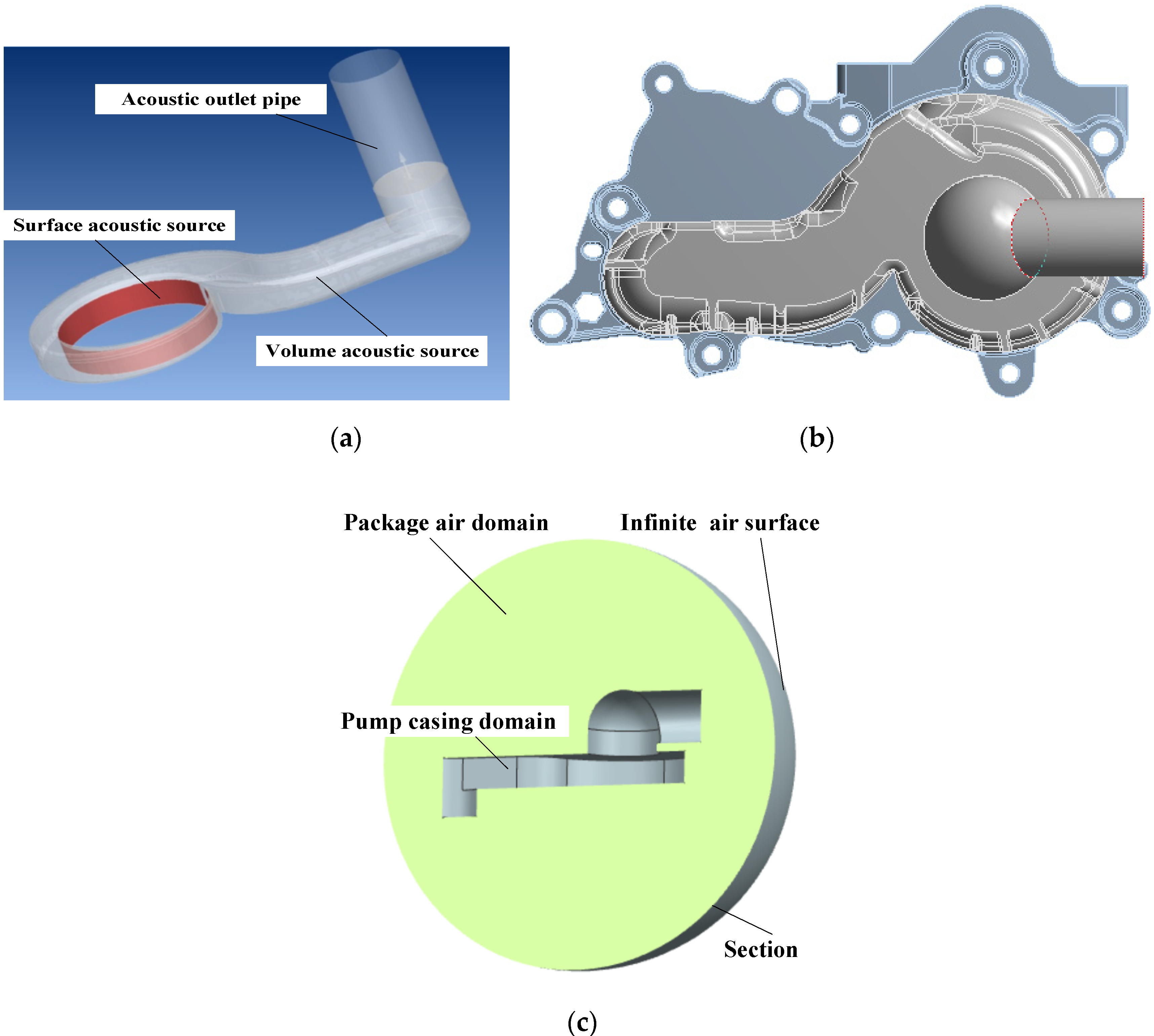
2.4.3. Computation setup of the acoustic field

There are three main computational domains for acoustic calculations (as shown in Figure 6) named water flow domain, pump casing structure, and air radiation sound fields.

The water flow domain and pump casing structure domain are coupled to process fluid-borne noise calculation. The inlet tube and rotating impeller are not included here, where sound source information calculated by CFD would be transferred to the volute import as a surface sound source. The volute water area is used as both acoustic generation area and the sound propagation area, and its exit is set to the outlet. The calculation of radiated noise has added package air domain and infinite element radiation surface. The pump casing structure domain is also used for modal calculations.

The acoustic source information obtained from CFD is transformed into computational acoustics through meshes. Source information of inlet pipe and rotating impeller are loaded into the interface between impeller and volute as a surface acoustic source. Additionally, the sound source information in the volute area is loaded into the volute domain itself as a volume acoustic source. In general, the acoustic grid is coarser than the CFD grid. This paper takes the integration solution of the CFD results on the acoustic mesh to ensure all information is conserved in the information transfer process, as shown in Figure 7. This work is done in the software Actran’s preprocessor iCFD. It provides the mean flow interpolation method when CFD nodes are localized in the acoustic mesh structure. Moreover, smoothing operations are available when the CFD mesh is coarser than the acoustic mesh at the boundary. In order to ensure the convergence of acoustic equations, it also regularizes the flow field and automatically removes the boundary layer computed in RANS simulation [28].

The minimum wavelength of the acoustic finite element calculation should include at least 6 mesh cells, as follows:

$$L_{\max }<\frac{c}{6f_{\max }}$$

(12)

where L_max—maximum mesh size for acoustic calculation, c—speed of sound, f_max—maximum frequency identified by acoustic calculation. The maximum frequency covered by the unsteady flow field calculation is 6750 Hz, which identifies the maximum frequency of acoustic calculation to 6750 Hz. The speed of sound in the air is 346 m/s when the temperature reaches 25 °C, and in the water, it is 1497 m/s. Then, the grid size of the acoustic propagation region should be less than 8.54 mm in the air domain and 36.96 mm in the water domain. The maximum grid size of the computational domain used in this paper is 0.0014 m, which can meet the requirements of grid size in the acoustic finite element calculation.

The calculation process of radiation noise is similar to that of the fluid-borne noise, but the interface between structure domain and air domain needs to be defined. The acoustic finite element calculation requires the setting of the boundary conditions. Modes of pipelines are added to the outlet pipe, and infinite space elements are added to model the infinite air surface during acoustic preprocessing settings so that the sound propagates from the inside to the outside without reflection. The pump casing structure represents an aluminum shell (PPS) of 3 mm thickness, and the material of the pump base plant is ADC. The properties of both mentioned materials are shown in

Table 1. Material properties of the structure domain.

Material	Density/(kg/m3)	Young’s Modulus/GPa	Poisson Ratio
PPS	1500	11.95	0.4
ADC	2700	71	0.33

. The calculated acoustic frequency range is 0~6757 Hz, and the frequency resolution is set to 11.3 Hz.

3. Experimental Results

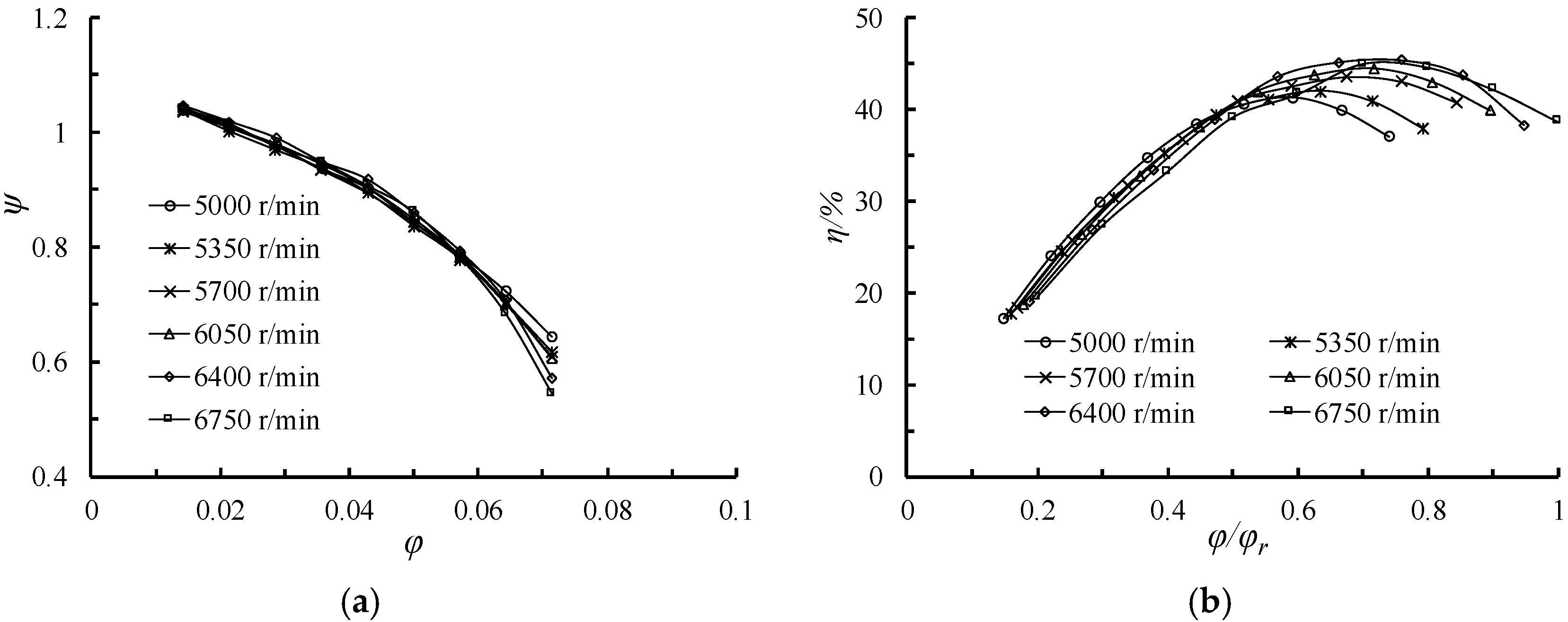
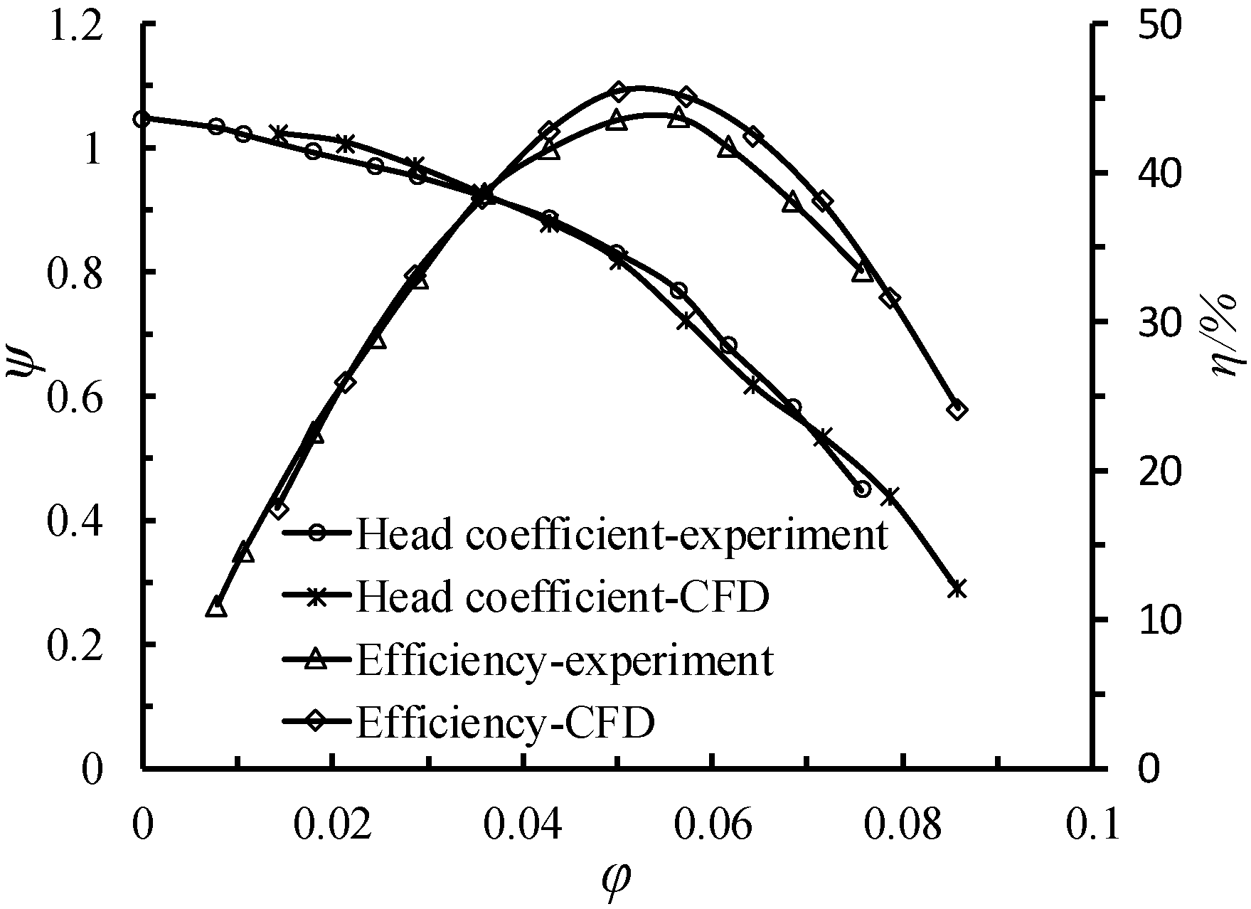
3.1. Overall Pump Performances

According to the similarity criterion, the external characteristic curve of the high-speed centrifugal pumps is dimensionless. The dimensionless flow rate formula and head formula are defined:

$$\phi =\frac{Q}{\pi d_2{b}_2{u}_2}$$

(13)

$$\psi =\frac{gH}{u_2^2/2}$$

(14)

where φ—flow rate coefficient, ψ—head coefficient, Q—flow rate, H—head, d₂—outlet diameter of the impeller, b₂—outlet width of the impeller, u₂—exit circumferential velocity of the impeller. The dimensionless pump performance curves at different rotational speeds are shown in Figure 8. φ_r represents the flow rate coefficient at Q_r. It can be seen that the dimensionless head and efficiency performance curves at different rotational speeds have high similarity, which means the internal flow in the pump also follows a similar law. However, the dimensionless head curve decreases faster at a large flow rate with the increase of rotating speed. These trends can be easily explained by the 1D Euler theory and the general knowledge of the flow phenomena taking place in the impeller under off-design operating conditions. The fluid inside the pump flows faster at higher rotating speed, which leads to more head loss. The high-efficiency area of the efficiency curve moves towards the direction of small flow, and the maximum value of efficiency decreases continuously with the decrease of rotational speed. This is because the operating point of the pump is also determined by the resistance of the circulation system, and the operation condition of the pump at low rotational speed offset to small flowrate (relative to the condition with maximum efficiency). Pumps produce more flow disturbances in the flow field under non-designed conditions. The internal flow is similar and that volume loss is less when the pump is working at a high rotational speed.

3.2. Analysis of Radiation Noise Characteristic

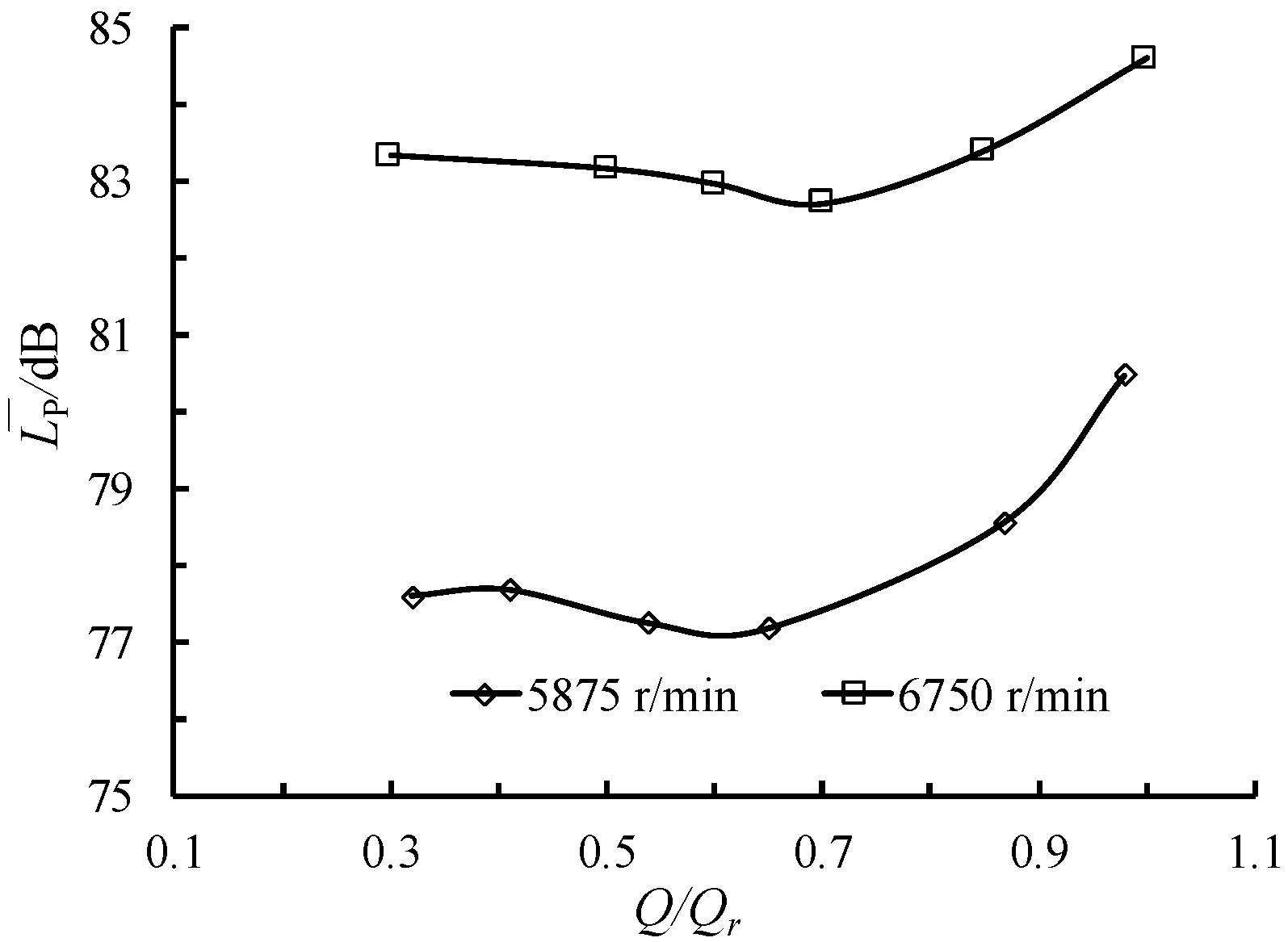
3.2.1. Sound Pressure Level at Different Flow Rates

The sound pressure level is a physical quantity that describes the response of the human ear to the intensity of the sound. The sound pressure level of the radiation noise from the model pump is measured at two rotational speeds of 5875 and 6750 r/ min, respectively, with the range from 0.3 to 1.0 Q_d. As can be seen from Figure 9, the sound pressure level curve increases slightly with the increase of the flow rate, then increases sharply after a small drop of the amplitude. Associated with the efficiency characteristic curves, the flow rate point that presents the minimum value of the sound pressure level corresponds to the highest efficiency area (0.7 Q_r). In general, the rotor–stator interaction, especially close to the volute tongue, may be considered a very significant energy dissipation mechanism and also the main fluid-borne noise source. When the pump is operating at a low flow rate, there is a clear wake-jet flow structure at the impeller outlet area. The greater extent in the velocity field fluctuation inside the blade channels would result in bigger fluid-borne noise. Increasing efficiency has a certain effect on reducing noise under this condition. When the flow rate exceeds the optimal working condition, the sound pressure level is increased greatly. On the one hand, this is due to the higher velocity level of the fluid in the pump at high flow rates, which causes a stronger rotor-stator interaction effect. Moreover, the coupling effect between the fluid and the structure is enhanced and the fluid load is also increasing, which could cause higher mechanical noise.

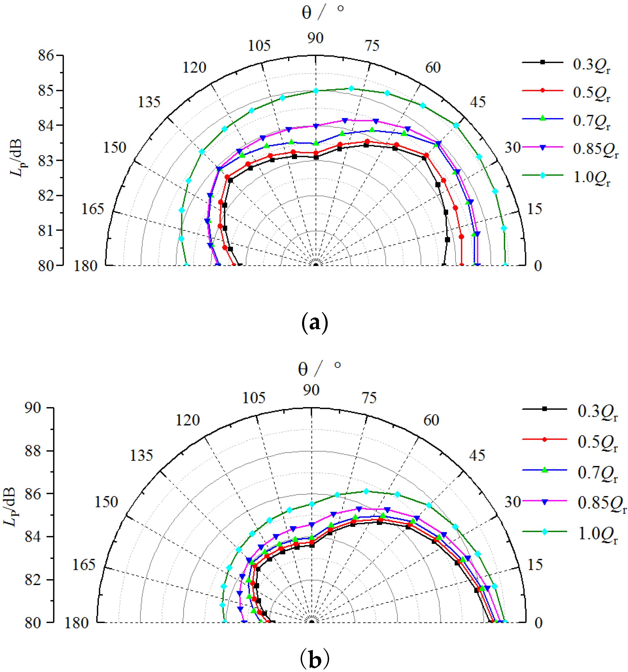
3.2.2. Acoustic Directivity at Different Flow Rates

The radiation noise intensity of the high-speed centrifugal pump under different flow conditions was measured with a rotation speed of 6750 r/min. The test was conducted in a semi-anechoic chamber, and the pump was fixed to a heavy foundation. Details such as the location of microphone sensors and pump position can be seen in Figure 3. In order to make the directivity feature more compatible with natural intuition, the directivity curves were plotted using linear interpolation, as shown in Figure 10. In the vertical direction, the directivity of the radiation noise shows quadrupole characteristics at a small flow rate and the polarity appears in 45 °and 135 °directions, respectively. The acoustic radiation expands outward, and the intensity increases gradually with the increase of flow rate. When the flow rate increases to 0.85 Q_r, the quadrupole shape of the characteristics becomes not so obvious, and the distribution of sound pressure level tends to be uniform at each measuring point. When the flow rate reaches Q_r, the polarity of 45°and 135° measuring points disappears, and the directivity curve shows the characteristics of dipoles. In view of the flow-induced noise mechanism, the backflow at the inlet and outlet of impeller and flow separation from the turbulence inside the flow-path can be regarded as a quadrupole sound source under a small flow rate. The increase of flow rate makes the flow field more uniform, which leads to the decrease of the contribution of the quadrupole sound source to the whole sound field. When the flow rate reaches the design operation point, the interaction between the moving fluid and the solid boundary is enhanced and the contribution of dipole sound source to the radiation noise increases, which becomes the main noise source. At 45° oblique direction, the directivity characteristics of radiation noise are not obvious, which indicates that the directivity characteristics of radiation noise are closely related to the spatial distribution.

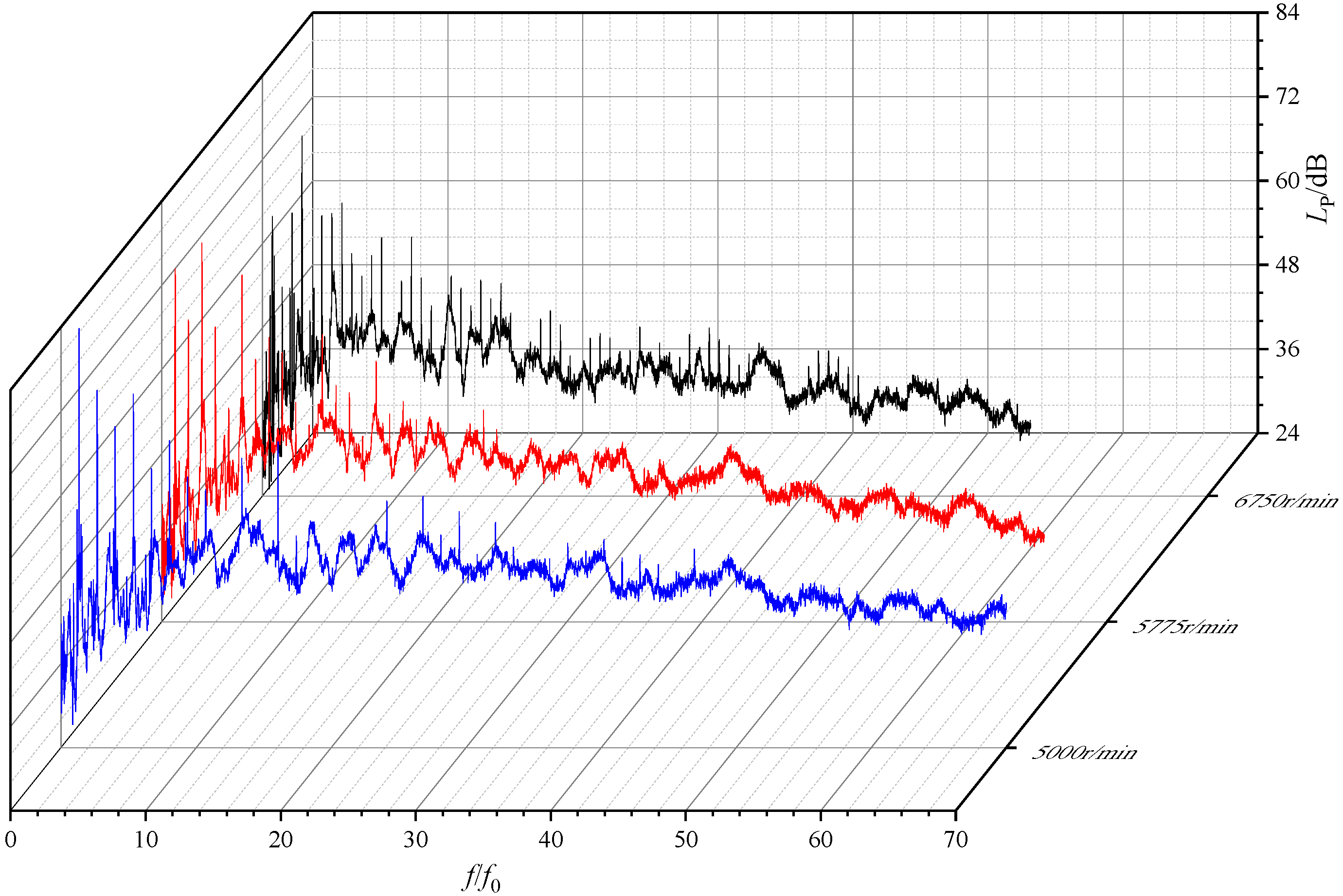
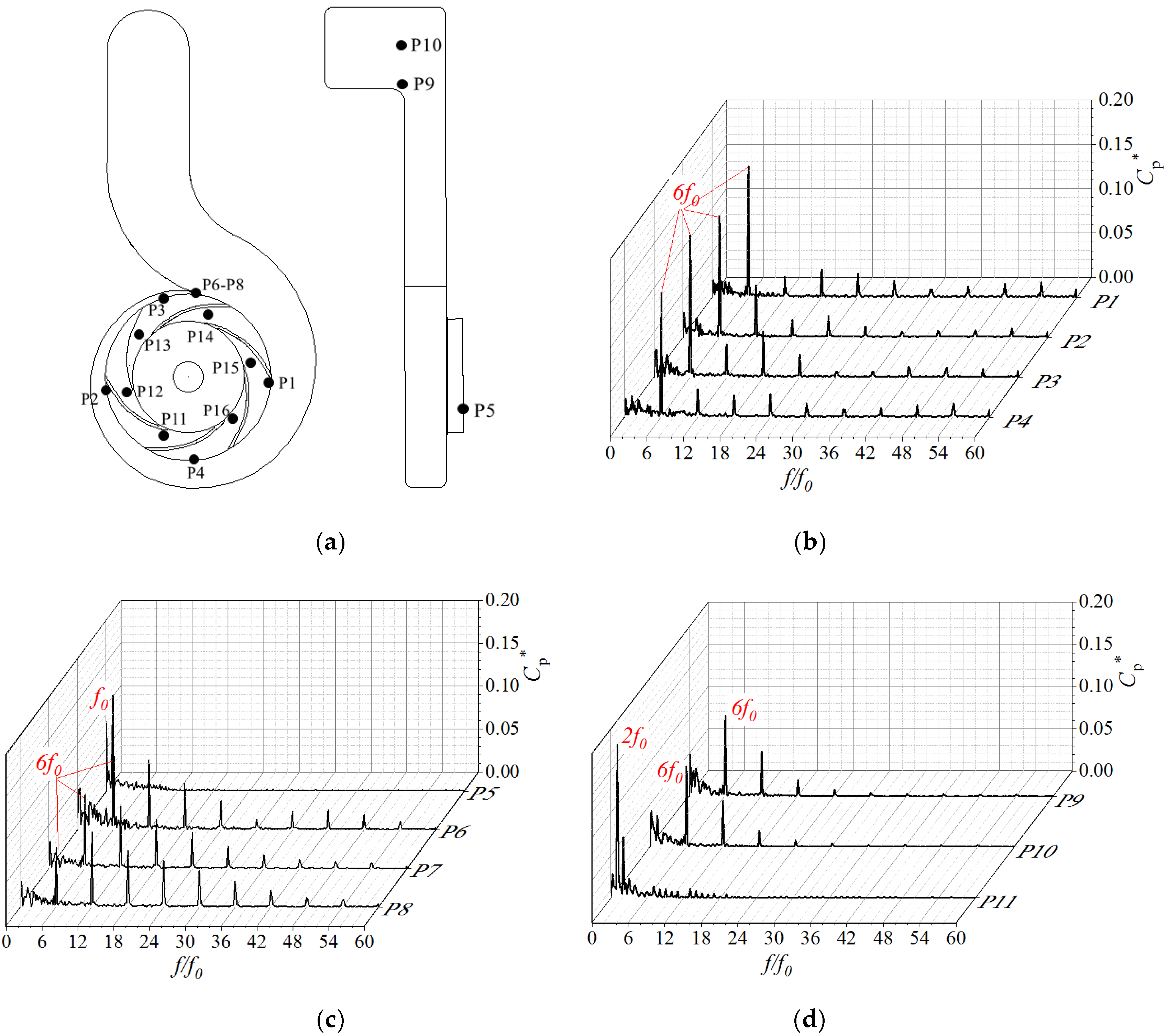
3.2.3. Frequency Domain Characteristics of the Radiate Noise

In order to measure the radiation noise characteristics of the pump under realistic operation conditions, the circulation system is adjusted to engine resistance characteristics, which means the model pump works at Q_r under 6750 r/min. Another two tests under 5875 and 5000 r/min rotational speed without changing the system resistance characteristics are also processed. Signals from microphone 3, located directly above the pipeline, are used to carry out frequency characteristics analysis. The cutoff frequency of the analysis is 6400 Hz. f₀ represents the fundamental frequency, which corresponds to the shaft rotation speed. As can be seen from Figure 11, the energy of the noise of all three rotational speed is mainly concentrated in the low-frequency region. At frequencies higher than 20f₀, the pressure level amplitudes decay rapidly. The noise spectral component shows obvious discreteness; its frequency is the shaft rotation frequency and its multiples. The SPL amplitude is the highest at the blade passing frequency (six times the shaft rotation frequency) because of the rotor–stator interaction influence. The discrete characteristics of the dimensionless frequency spectrum at three pump rotational speed demonstrate the same, so the next numerical simulation can only focus on the situation of 6750 r/min.

4. Numerical Results Analysis

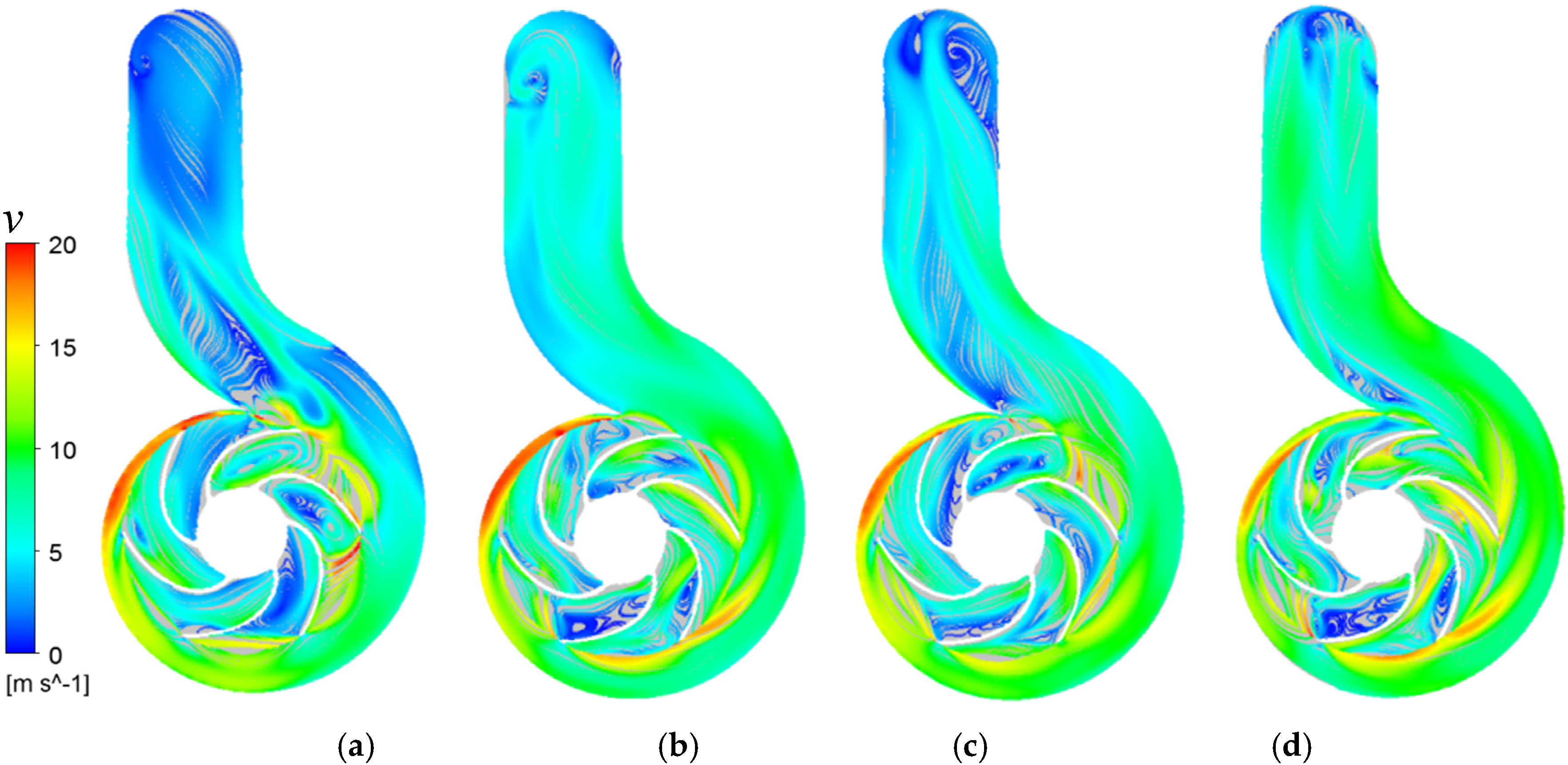
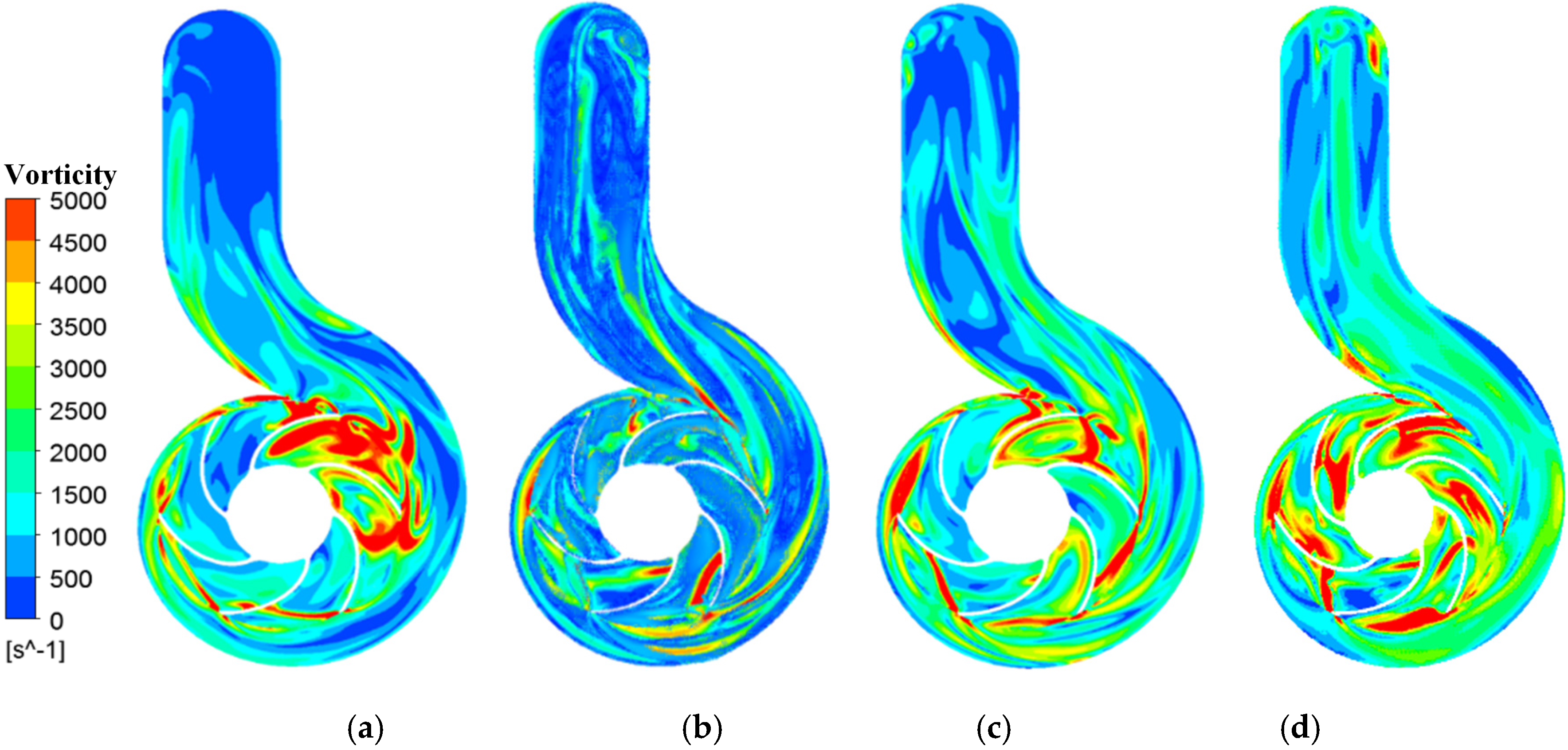
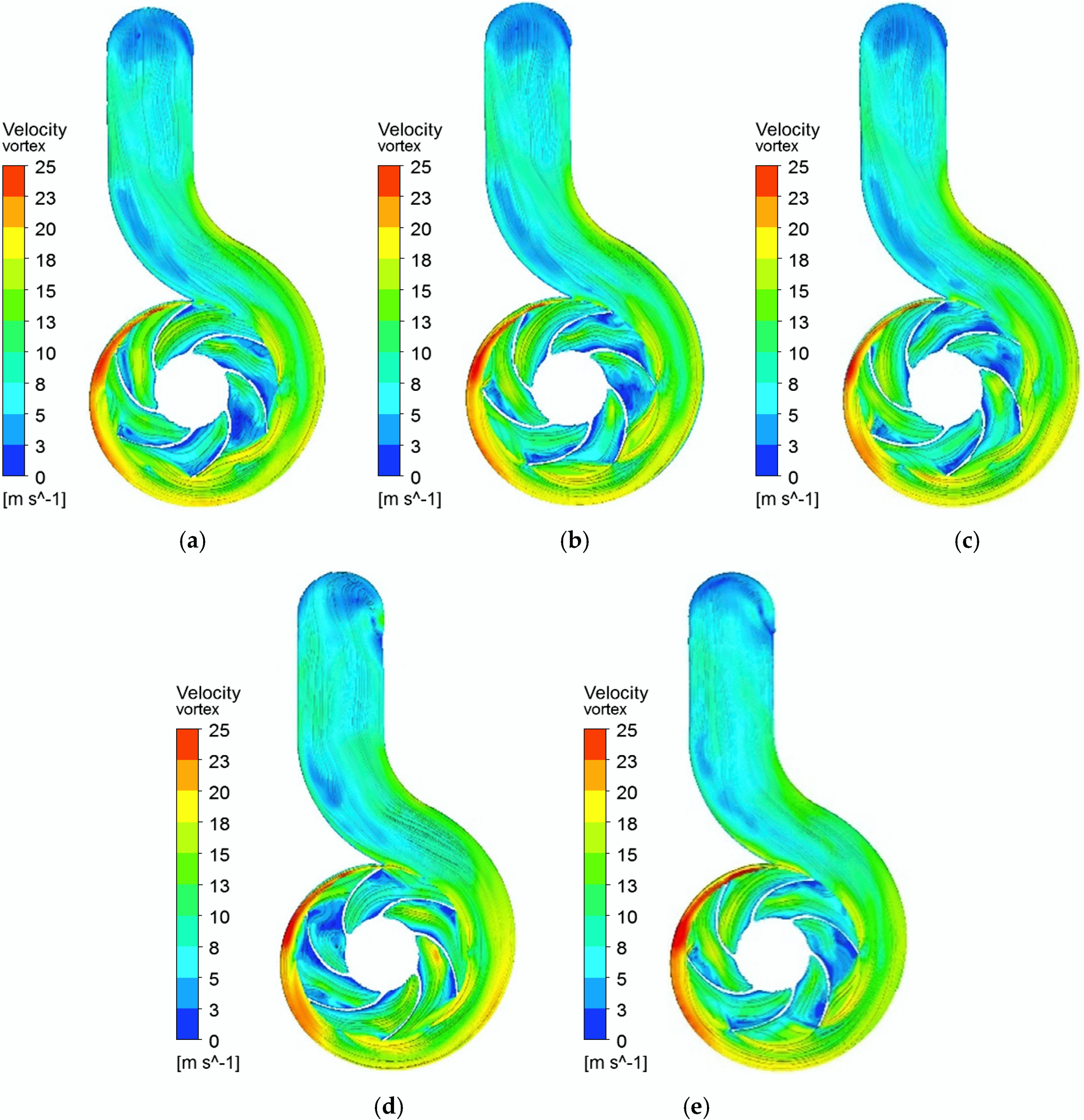
4.1. Flow Field Results Analysis

A comparison of pump performance between the simulation and experimental results is shown in Figure 12 under 6750 r/min. Q_r is equivalent to the flow rate coefficient C_q = 0.0715. Seen from the figure, the simulated and experimental values of both the head coefficient and efficiency are almost the same at Q_r. The maximum error between the test value and the simulated value of the head coefficient is below 5.5% for the full flow rate. From the simulated efficiency curve, the operation point with the highest efficiency is near 0.7Q_r. At the small flow rate condition, the test value of efficiency is close to the simulated ones. The maximum error is not higher than 4.3% for the full flow rate. Therefore, the selected calculation model used in the simulation can be considered to accurately predict the performance of the pump and could be used to translate pump internal flow information for further analysis.

The absolute velocity distribution of the model pump flow field under different flow conditions are presented in Figure 13. As seen from the figure, the fluid velocity appears the highest at impeller exit and shows asymmetry on the circumference due to the rotor–stator interaction caused by the volute tongue. Under all presented flow conditions, swirls appear inside the impeller flow channel, especially at the suction side of blade leading edge and pressure side of the blade trailing edge. At the flow rate exceeding the highest efficiency working point (0.7Q_r), the number of vortices gradually increased, and the size continued to expand, which severely affected the impeller operation and caused noise problems. In addition to 0.7Q_r, flow separation near the volute tongue also occurred, which also became a source of flow-induced noise. The special structure of the exit with a 90° corner also caused a vortex, which resulted in a significant hydraulic problem.

Vorticity is often used to represent the curl characteristic of a flow field. The swirling motion in the fluid medium is the source of flow-induced noise based on the vortex sound theory [20]. The vorticity distributions of the model pump’s flow field under different flow conditions are presented in Figure 14. It can be seen that high-energy vortices are mostly concentrated near the velocity vortex areas of the flow field, such as the rotor–stator interaction zones and flow separation zones inside the blade channel. The highest efficiency working conditions present the least distribution of high energy vorticity. The working condition appeared as the least distribution of high energy vorticity at 0.7Q_r. Due to insufficient flow, large areas of backflow and secondary flow exist in the impeller flow channel at a low flow rate (0.5Q_r), showing relatively high vorticity and asymmetric distribution. Under large flow conditions, the vortex diffuses into the impeller flow channel, which is related to the high-speed area at the leading edge of impeller blade. In addition, a small amount of high-energy vortex mass also appears at the exit of the volute. When the vorticity moves in the same direction of the mean flow inside the rotational impeller, the energy dissipation rate on the blade surface will be reduced. On the contrary, it is not conducive to the fluid energy conversion between the impeller and the volute, which explains the head and efficiency dropping at large flow rates. To be fair, the hydraulic design of this model pump is not excellent due to space constraints, resulting in lower hydraulic efficiency and vibration and noise problems.

4.2. Unsteady Flow Characteristic Analysis

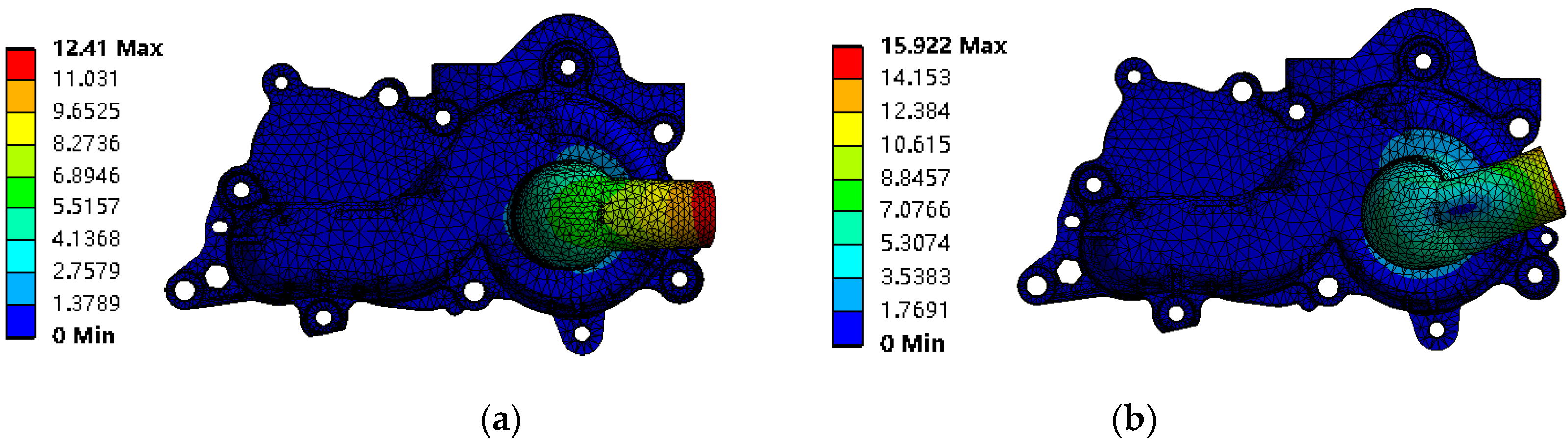
In order to study the pressure pulsation of the model pump, 16 virtual monitoring points are set in the middle section of the pump from the inlet pipe to the outlet of the volute during the simulation process, and the dimensionless pressure coefficient C_p is introduced to characterize the pressure pulsation intensity at each monitoring point [29]. C_p is defined by Equation (15), with p denoting the static pressure and p standing for the averaged static pressure.

$$C_P=\frac{\left(p-\overline{p}\right)}{0.5\rho u_2{}^2}$$

(15)

After applying the FFT (fast Fourier transform) to C_p in the time domain, the frequency domain amplitude coefficients C_p^*of the pressure pulsation at every monitoring point are obtained. The trusted sampling frequency is 6756 Hz based on DES unsteady calculation, which could cover the analysis frequency range of flow-induced noise from the experiment information. The location and spectrum of the monitoring points are shown in Figure 15. As seen from it, the spectrum curves present discrete characteristics; the main frequency of mostly monitoring points is blade passing frequency (6f₀ = 675 Hz) and its multiple due to the rotor–stator interaction between the impeller and the volute. The characteristic frequency is concentrated in the low-frequency region; the pulsation peak decreases after increasing above the threshold of 30f₀. C_p^* appears largest at the impeller exit area, especially around the volute tongue (P6, P7, P8). Affected by unstable flow phenomena such as flow separation and stall in the impeller, pulsations also obviously exist below 6f₀. The main frequency of P11 located at the inlet of the impeller blade is 2f₀, which may be due to the stall phenomenon in the flow channel. The main frequencies of P9 and P10 are also 6f₀, which indicates that the pump’s outlet pressure wave propagation is characterized by rotor–stator interaction as dipole characteristics.

In order to understand the flow characteristics of the pump more clearly, the velocity vortex distribution located on the middle span of the pump in one blade passing time is shown in Figure 16. The symbol t₀ presents the moment that one blade passes the volute tongue. T means 1/(6f₀). The shape and size of the flow vortex in each of the six flow-paths are different and there is relative motion with the direction of impeller rotation. The flow field does not change much from the volute tongue to the pump outlet during a blade passing time. Many flow pulsations occur with a period higher than one blade passage time, which is reflected by the low-frequency characteristic of the pressure pulsation for each monitoring point. Low-speed vortices areas are generated, developed, and disappear in the impeller flow path and, mostly, at the impeller outlet. The velocity varies greatly at the impeller blade inlet, which corresponds to the peak value of pressure pulsation amplitude at P11. The main reason for the change of the flow field is still the unsteady flow of the impeller and rotor–stator interaction between the blade and the volute tongue.

4.3. Modal Analysis

The grid division of structure domain, material selection, and calculation execution is carried out in Ansys Workbench14.1. Because the cooling pump is mainly connected to the base of the internal combustion engine by 12 bolts, the simulation restrains the 12 holes and assumes thesurface of the inlet pipe as a fix in the pretreatment for the model calculation to obtain natural frequency and mode of vibration. The first 10-order natural frequencies are shown in

Table 2. Natural frequency of the pumps structure.

Mode	Natural Frequency/Hz	Mode	Natural Frequency/Hz
1st mode	928.29	6th mode	3702.2
2nd mode	1095.7	7th mode	3840.5
3rd mode	2045.2	8th mode	4767.8
4th mode	2932.3	9th mode	5089
5th mode	3670.6

, and the selected first and fourth order model shapes of pump structure are shown in Figure 17.

There are 9th-order natural frequencies below 5200 Hz; the third-order natural frequency is 2045.2 Hz, which is relatively close to triple the blade passing frequency (675 Hz). It is necessary to pay attention to avoid possible resonance. From the view of mode shapes, the deformation of the pump casing mainly occurs at the inlet tube and the volute tongue. The inlet pipe shows the greatest deformation due to the relatively thin connection at this location. The possibility to induce resonance phenomenon by fluid excitation force is small due to the pressure pulsation is being mainly concentrated in the low-frequency region.

4.4. Acoustic Field Results Analysis

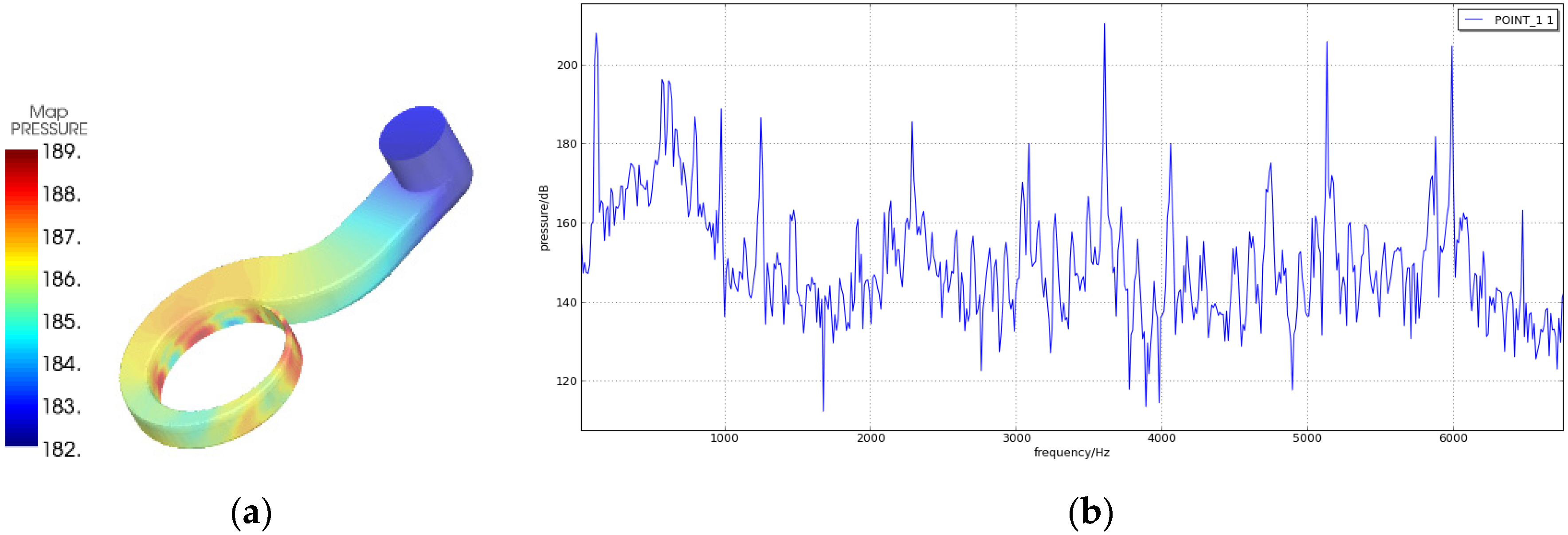
4.4.1. Fluid-Borne Noise

The flow data file of the last 10 impeller rotation cycles (including the pressure, velocity, and fluid density values) is used as the initial sound source file for the hydrodynamic noise calculation at Q_r. The coupling effect of the pump shell is considered in the simulation. Distribution map of sound pressure level and the spectrum curve of field point located at the pump outlet are shown in Figure 18. It can be seen from the figure that the sound pressure level is steadily decreasing from volute inlet to volute outlet. The regions with the highest sound pressure level are distributed at the impeller outlet, especially the volute tongue area. That might be because of the rotor-stator interaction between the rotating impeller and stationary volute. Flow-path space of the spiral volute start from the first cross-section is increased and eventually becomes big enough for the passing fluid, which results in weakening of sound source intensity. The frequency spectrum of predicted noise is dominated by discrete frequencies. The sound pressure level in the low-frequency area is relatively high overall; f₀ and 6f₀ (675Hz) are the main frequencies, which are consistent with the aforementioned noise test and flow field simulation results. There are relatively large peaks between 3000–6000 Hz, which might be due to the coupling of the pump shell and the vibro-acoustic interaction.

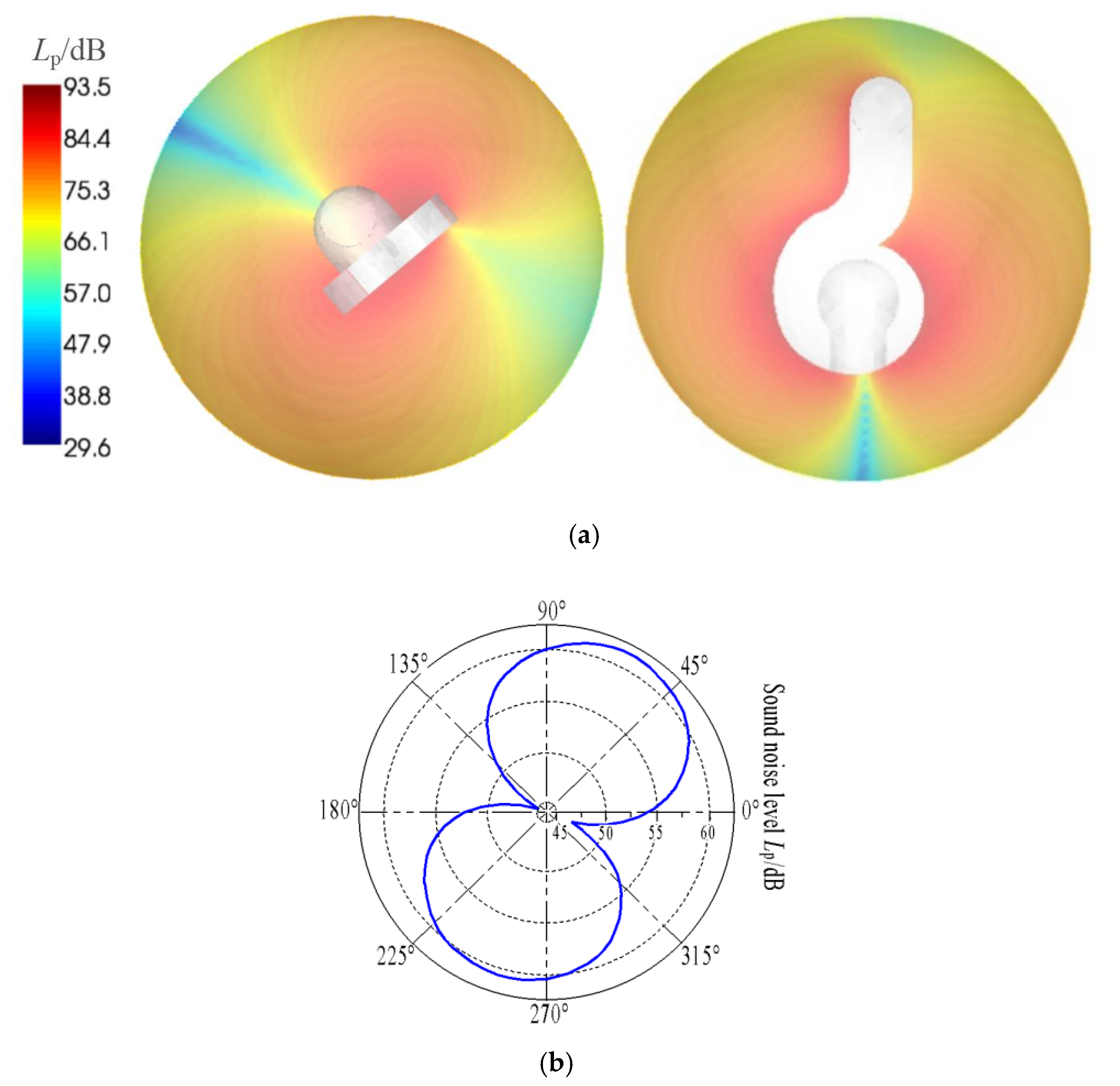
4.4.2. Fluid-Induced Radiated Noise

Radiated noise calculations are performed on the basis of fluid-borne noise calculations after adding the air domain and establishing the infinite element boundary conditions at the radiated air surface. A cloud map and a directivity curve of the radiated noise are shown in Figure 19. Orientation and location are set as the same to the experiment, as shown in Figure 3. Unlike the experimental results, it shows full-space curves, while the experiment could only show half-space curves because of ground constraints. Figure 19a shows the sound pressure level distribution of the model pump at vertical impeller midsection (left) and parallel impeller midsection (right). Figure 19b presents the directive curve obtained by interpolating the sound pressure level values of the monitoring points. the radiated noise level of the color chart based on the value.

Seen from the figure, both the cloud map and the directivity diagram of radiation noise corresponding to blade-passing frequency show dipole characteristics (“8 shape”), which is confirmed by the previous radiation noise test. It indirectly means that the pressure fluctuation caused by the rotor–stator interaction between the impeller and volute is the main source of the radiation noise because there is a conversion of energy taking place here. The sound pressure level of radiation noise in the air domain presents the highest near the pump shell surface and decreases along the radial direction. From the forward direction of the cloud diagram, the gradient of the sound pressure level is small. The light blue band area formed at the entrance pipe indicates that the flow instability is more pronounced at the impeller inlet area. In general, the CFD/CFA method used in this paper provides an accurate estimate of the flow-induced noise characteristics under the design operation point. However, stimulation in the form of velocity field fluctuations comes from the inner blade channels and acoustic effects at off-design (overload) point of operation would be very high, which needs more consideration in the future.

5. Conclusions

An open type system is built in a semi-anechoic room as a test rig to study performance and radiated noise characteristics of a high-speed centrifugal pump under different rotational speed. A CFD/CFA calculation method is proposed to predict the fluid-borne noise and radiated noise characteristics. Experimental and numerical analyses were performed on the model pump for flow-induced noise characteristics. The main conclusions are the following:

1. In the speed range of 5000–6750 r/min, pump performance conforms to similar laws; the dimensionless head curve is basically the same at different speeds. With decreases of rotational speed, the zone with high value in the efficiency becomes narrow and moves to small flow rate area, and the highest value of efficiency gets continuously reduced. The dimensionless radiated noise also conforms to a similar law, and the highest efficiency point pump presents the lowest noise level.

2. Based on Lighthill’s acoustic analogy theory, the proposed CFD/CFA method is proven effective to calculate the fluid-borne noise and flow-induced radiated noise of the model pump. The DES model could give accurate sound-source information. Considering the coupling effect of the structure field, the predicted radiation sound field exhibited dipole characteristics combined with the acoustic finite element method. Consistent with the experimental results, the predicted noise spectrum of pump required flow rate shows broadband characteristics but with obvious discrete peaks, which are not only related to the fluid sound source (6f₀) at the low-frequency region, but also to the natural vibration frequency of the structural mode (3000–6000 Hz region).

3. The main frequency of the pressure pulsation in the flow field presents blade passing frequency (6f₀), which further causes the radiated noise to show dipole characteristics. Therefore, rotor–stator interaction between the rotating impeller and stationary volute of the pump flow field is the main cause of flow-induced noise. The unstable flow such as the stall vortex in the pump impeller and the flow separation in the tongue area lead to the broadband characteristics of pressure pulsation concentrated at the low-frequency region, which also present in the noise spectrum.

References

1. Gülich, J.F. Centrifugal Pumps, 3rd ed.; Springer: Berlin/Heidelberg, Germany, 2014. [Google Scholar]
2. Guo, C.; Gao, M.; He, S.Y. A review of the flow-induced noise study for centrifugal pumps. Appl. Sci. 2020, 10, 1022. [Google Scholar] [CrossRef] [Green Version]
3. Wu, Y.L.; Li, S.C.; Liu, S.H.; Dou, H.S.; Qian, Z.D. Vibration of Hydraulic Machinery; Springer: Dordrecht, The Netherlands, 2013. [Google Scholar]
4. Zhong, S.Y.; Huang, X. A review of aero acoustics and flow-induced noise: For beginners. Acta Aero Dyn. Sin. 2018, 36, 363–371. [Google Scholar]
5. Lighthill, M. On sound generated aerodynamically: I. general theory. Proc. R. Soc. Lond. 1954, 222, 1–32. [Google Scholar]
6. Si, Q.R.; Ali, A.; Yuan, J.P.; Fall, I.; Muhammad, F.Y. Flow-induced noises in a centrifugal pump: A review. Sci. Adv. Mater. 2019, 11, 909–924. [Google Scholar] [CrossRef]
7. Simpson, H.C.; Macaskill, R.; Clark, T.A. Generation of hydraulic noise in centrifugal pumps. Proc. Instn. Mech. Engrs. 1966, 181, 84–108. [Google Scholar]
8. Chu, S.M.; Dong, R.Y.; Katz, J. Relationship between unsteady flow pressure fluctuations and noise in a centrifugal pump. Part A: Effects of blade-tongue interactions. J. Fluid Eng.-T ASME 1995, 117, 24–29. [Google Scholar] [CrossRef]
9. Chu, S.M.; Dong, R.Y.; Katz, J. Relationship between unsteady flow pressure fluctuations and noise in a centrifugal pump. Part B: Effects of blade-tongue interactions. J. Fluid Eng.-T ASME 1995, 117, 30–35. [Google Scholar] [CrossRef]
10. Choi, J.S.; Mclaughlin, D.K.; Thompson, D.E. Experiments on the unsteady flow field and noise generation in a centrifugal pump impeller. J. Sound Vib. 2003, 263, 493–514. [Google Scholar] [CrossRef]
11. Černetič, J. The use of noise and vibration signals for detecting cavitation in kinetic pumps. Proc. Inst. Mech. Eng. C 2009, 223, 1645–1655. [Google Scholar] [CrossRef]
12. Langthjem, M.A.; Olhoff, N. A numerical study of flow-induced noise in a two-dimensional centrifugal pump, Part II. Hydroacoustics. J. Fluid Struct. 2004, 19, 369–386. [Google Scholar] [CrossRef]
13. Parrondo, J.; Pérez, J.; Barrio, R.; Gonzales, J. A simple acoustic model to characterize the internal low frequency sound field in centrifugal pumps. Appl. Acoust. 2011, 72, 59–64. [Google Scholar] [CrossRef]
14. Keller, J.; Barrio, R.; Parrondo, J.; Barrio, R.; Fernandez, J.; Blanco, E. Effects of the pump-circuit acoustic coupling on the blade-passing frequency perturbations. Appl. Acoust. 2014, 76, 150–156. [Google Scholar] [CrossRef]
15. Mao, X.L.; Pavesi, G.; Chen, D.Y. Flow induced noise characterization of pump turbine in continuous and intermittent load rejection processes. Renew. Energy 2019, 139, 1029–1039. [Google Scholar] [CrossRef]
16. Jiang, Y.Y.; Yoshimura, S.; Imai, R.; Katsura, H.; Yoshida, T.; Kato, C. Quantitative evaluation of flow-induced structural vibration and noise in turbomachinery by full-scale weakly coupled simulation. J. Fluid Struct. 2007, 23, 531–544. [Google Scholar] [CrossRef]
17. Si, Q.R.; Shen, C.H.; Ali, A.; Cao, R.; Yuan, J.P.; Wang, C. Experimental and numerical study on gas-liquid two-phase flow behavior and flow induced noise characteristics of radial blade pumps. Process 2019, 7, 920. [Google Scholar] [CrossRef] [Green Version]
18. Si, Q.R.; Wang, B.B.; Yuan, J.P.; Huang, K.L.; Lin, G.; Wang, C. Numerical and experimental investigation on radiated noise characteristics of the multistage centrifugal pump. Processes 2019, 7, 793. [Google Scholar] [CrossRef] [Green Version]
19. Kapellos, C.S.; Papoutsis-Kiachagias, EM.; Giannakoglou, K.C.; Hartmann, M. The unsteady continuous adjoint method for minimizing flow-induced sound radiation. J. Comput. Phys. 2019, 392, 368–384. [Google Scholar] [CrossRef] [Green Version]
20. Velarde, S.; Tajadura, R. Numerical simulation of the aerodynamic tonal noise generation in a backward-curved blades centrifugal fan. J. Sound Vib. 2006, 295, 781–786. [Google Scholar]
21. Cravero, C.; Marsano, D. Numerical Prediction of Tonal Noise in Centrifugal Blowers. In Proceedings of the Turbo Expo 2018: Turbomachinery Technical Conference & Exposition, Oslo, Norway, 11–15 June 2018. [Google Scholar]
22. Caro, S.; Ploumhans, P.; Gallez, X. Implementation of Lighthill’s Acoustic Analogy in a Finite/Infinite Elements Framework. In Proceedings of the 10th AIAA/CEAS Aeroacoustics Conference, Manchester, UK, 10–12 May 2004. [Google Scholar]
23. International Organization for Standardization (ISO). ISO 9906: 2012 Rotodynamic Pumps-Hydraulic Performance Acceptance Tests—Grades 1, 2 and 3; ISO: Geneva, Switzerland, 2012. [Google Scholar]
24. Si, Q.R.; Lu, R.; Shen, C.H.; Xia, S.J.; Sheng, G.C.; Yuan, J.P. An intelligent CFD-based optimization system for fluid machinery: Automotive electronic pump case application. Appl. Sci. 2020, 10, 366. [Google Scholar] [CrossRef] [Green Version]
25. Huang, K.; Yuan, J.; Si, Q.; Lin, G. Numerical simulation on pressure pulsation in multistage centrifugal pump under several working conditions. J. Drain. Irrig. Mach. Eng. 2019, 37, 387–392. [Google Scholar]
26. Strelets, M. Detached Eddy Simulation of Massively Separated Flows. In Proceedings of the 39th Aerospace Sciences Meeting and Exhibit, Reno, NV, USA, 8–11 January 2001. [Google Scholar]
27. Si, Q.; Bois, G.; Liao, M.; Zhang, H.; Cui, Q.; Yuan, S. A comparative study on centrifugal pump designs and two-phase flow characteristic under inlet gas entrainment conditions. Energies 2020, 13, 65. [Google Scholar] [CrossRef] [Green Version]
28. Free Field Technologies Co. MSC Actran14.1 User’s Guide; Free Field Technologies, Co.: Mont-Saint-Guibert, Belgium, 2012. [Google Scholar]
29. Yang, J.; Xie, T.; Liu, X.H.; Si, Q.R.; Liu, J. Study of unforced unsteadiness in centrifugal pump at partial flow rates. J. Therm Sci. 2019. [Google Scholar] [CrossRef]
Figure 1. Three-dimensional structure of high-speed centrifugal pump model.
Applsci 10 03105 g001
Figure 2. The flow chart of the radiated noise analysis of the high-speed centrifugal pump.
Applsci 10 03105 g002
Figure 3. Test Rig: (a) test loop (b) microphone placement; (c) test scene.
Applsci 10 03105 g003aApplsci 10 03105 g003b
Figure 4. Analysis of mesh independence.
Applsci 10 03105 g004
Figure 5. Computational domains and generated meshes of the model pump.
Applsci 10 03105 g005
Figure 6. The sound field calculation: (a) water flow domain; (b) pump casing structure; (c) air radiation sound fields.
Applsci 10 03105 g006
Figure 7. Grid interpolation method: (a) integration solution; (b) solution at boundary.
Applsci 10 03105 g007
Figure 8. Pump performance curves at different rotational speed: (a) dimensionless head curve; (b) pump efficiency curves.
Applsci 10 03105 g008
Figure 9. Variation of radiated noise at different speeds.
Applsci 10 03105 g009
Figure 10. Half directivity characteristics curves of radiated noise at different operating conditions: (a) vertical direction; (b) skew 45 °direction.
Applsci 10 03105 g010
Figure 11. Contrast chart of frequency spectrum under the full opening of the valve.
Applsci 10 03105 g011
Figure 12. Hydraulic characteristics of numerical calculation and experiment.
Applsci 10 03105 g012
Figure 13. Velocity streamline line of model pump: (a) 0.5 Qr, (b) 0.7 Qr, (c) 1.0 Qr, (d) 1.2Qr.
Applsci 10 03105 g013
Figure 14. Vortex distribution of model pump: (a) 0.5 Qr, (b) 0.7 Qr, (c) 1.0 Qr, (d) 1.2 Qr.
Applsci 10 03105 g014
Figure 15. Spectrum of pressure fluctuation in the cooling pump at Qr: (a) monitoring points location; (b) pressure spectrum of P1–P4; (c) pressure spectrum of P5–P8; (d) pressure spectrum of P9–P11.
Applsci 10 03105 g015
Figure 16. Velocity vortex distribution under Qr: (a) t = t0; (b) t = t0 + 1/2T; (c) t = t0 + T; (d) t = t0 + 3T; (e) t = t0 + 5.5T.
Applsci 10 03105 g016
Figure 17. Mode shapes of pumps structure with amplitude unit mm: (a) 1st mode; (b) 4th mode.
Applsci 10 03105 g017
Figure 18. Fluid-borne noise characteristics at Qr: (a) the Lp contour at 6f0 with unit dB; (b) spectrum curve.
Applsci 10 03105 g018
Figure 19. Radiated noise characteristics under 6f0: (a) cloud map; (b) directivity and radiated noise level curve.
Applsci 10 03105 g019