Fatigue Evaluation of Steel Bridge Details Integrating Multi-Scale Dynamic Analysis of Coupled Train-Track-Bridge System and Fracture Mechanics

Abstract
:Featured Application
Abstract
1. Introduction
2. Multi-Scale Bridge FE Model
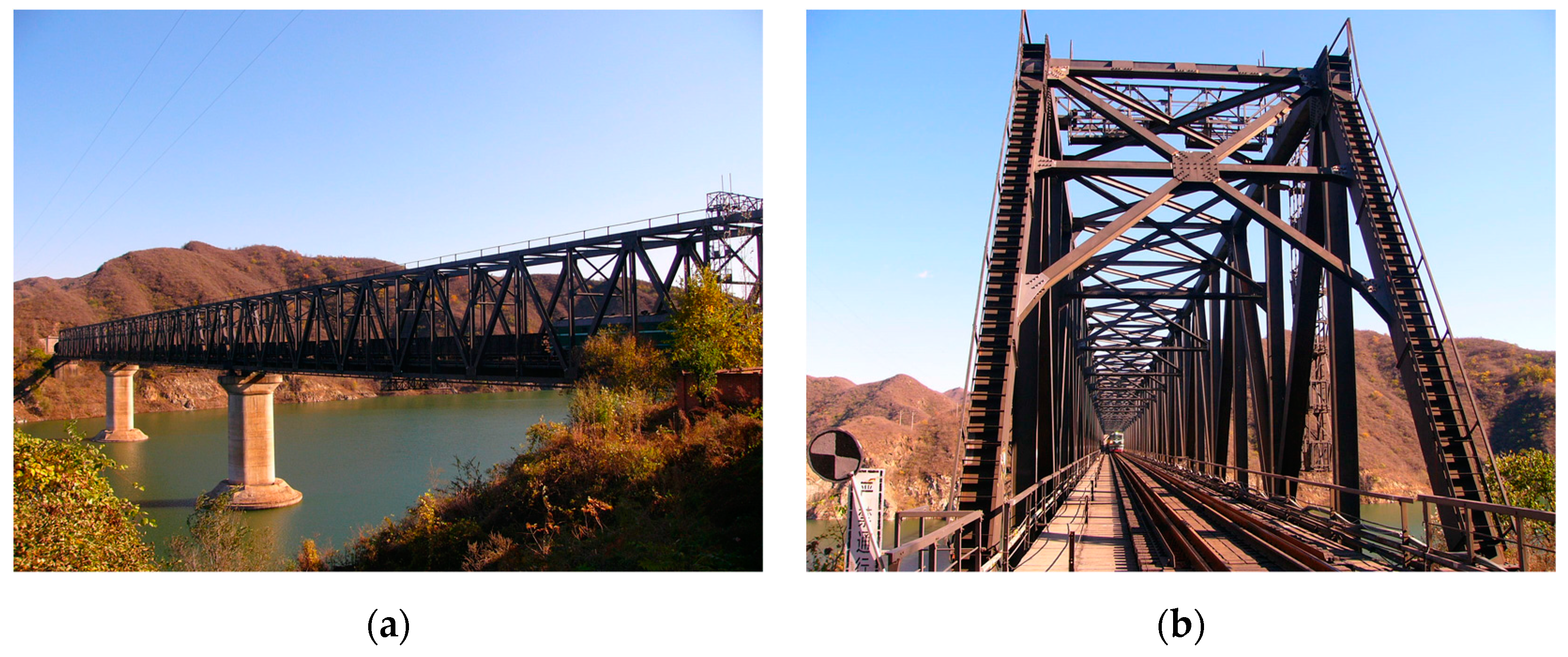
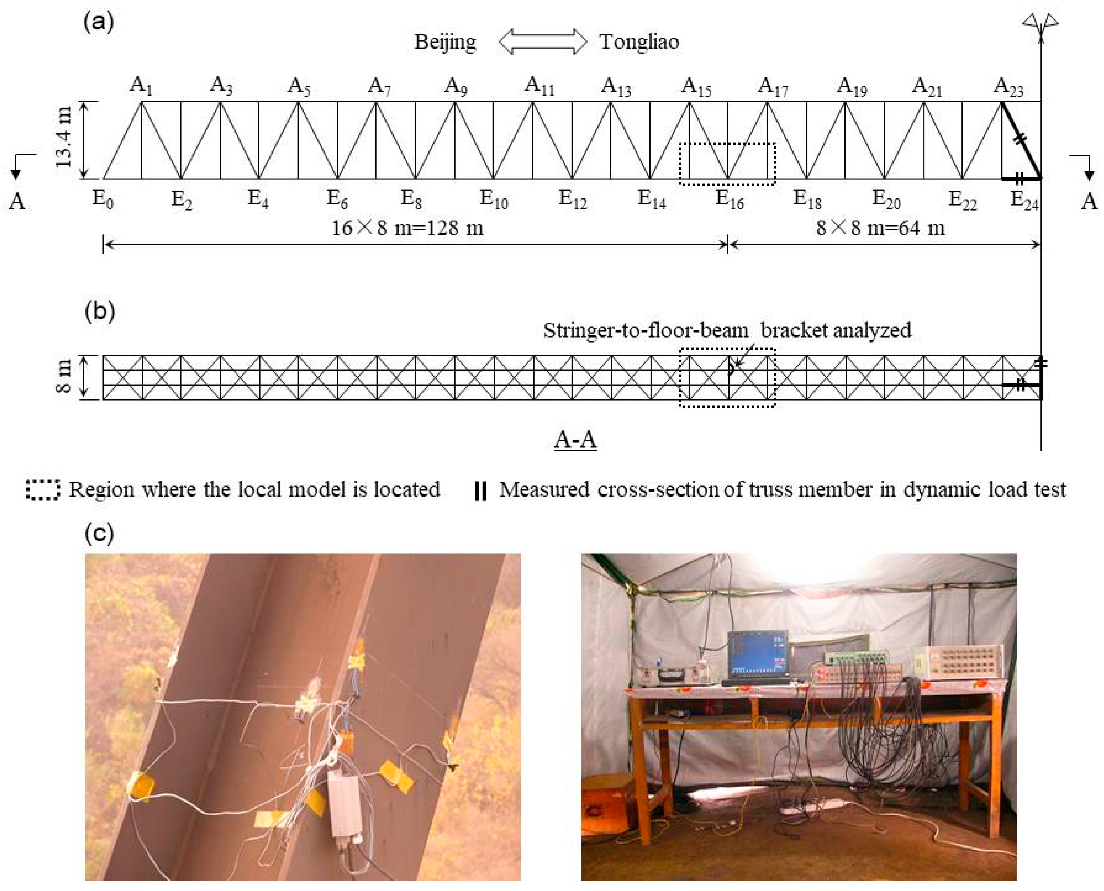
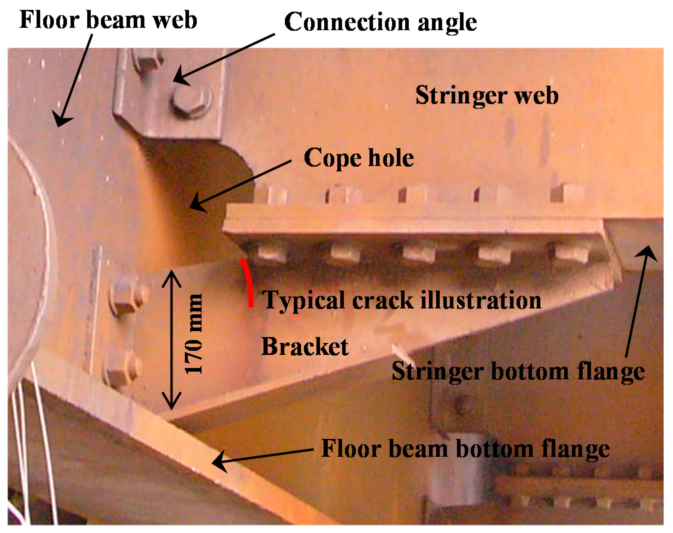
2.1. Engineering Background
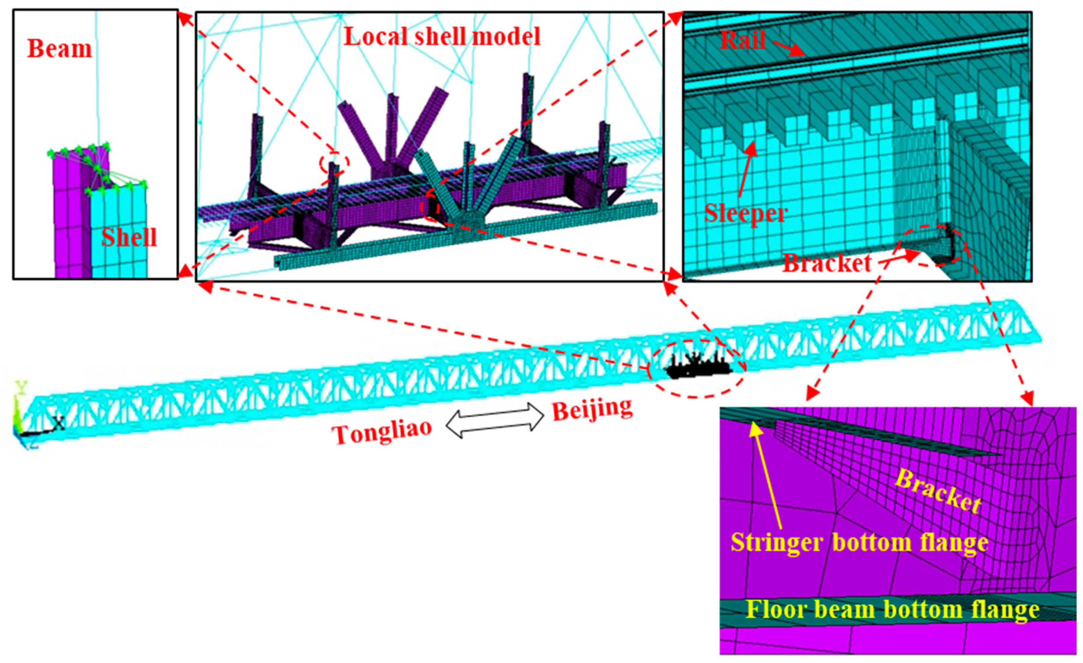
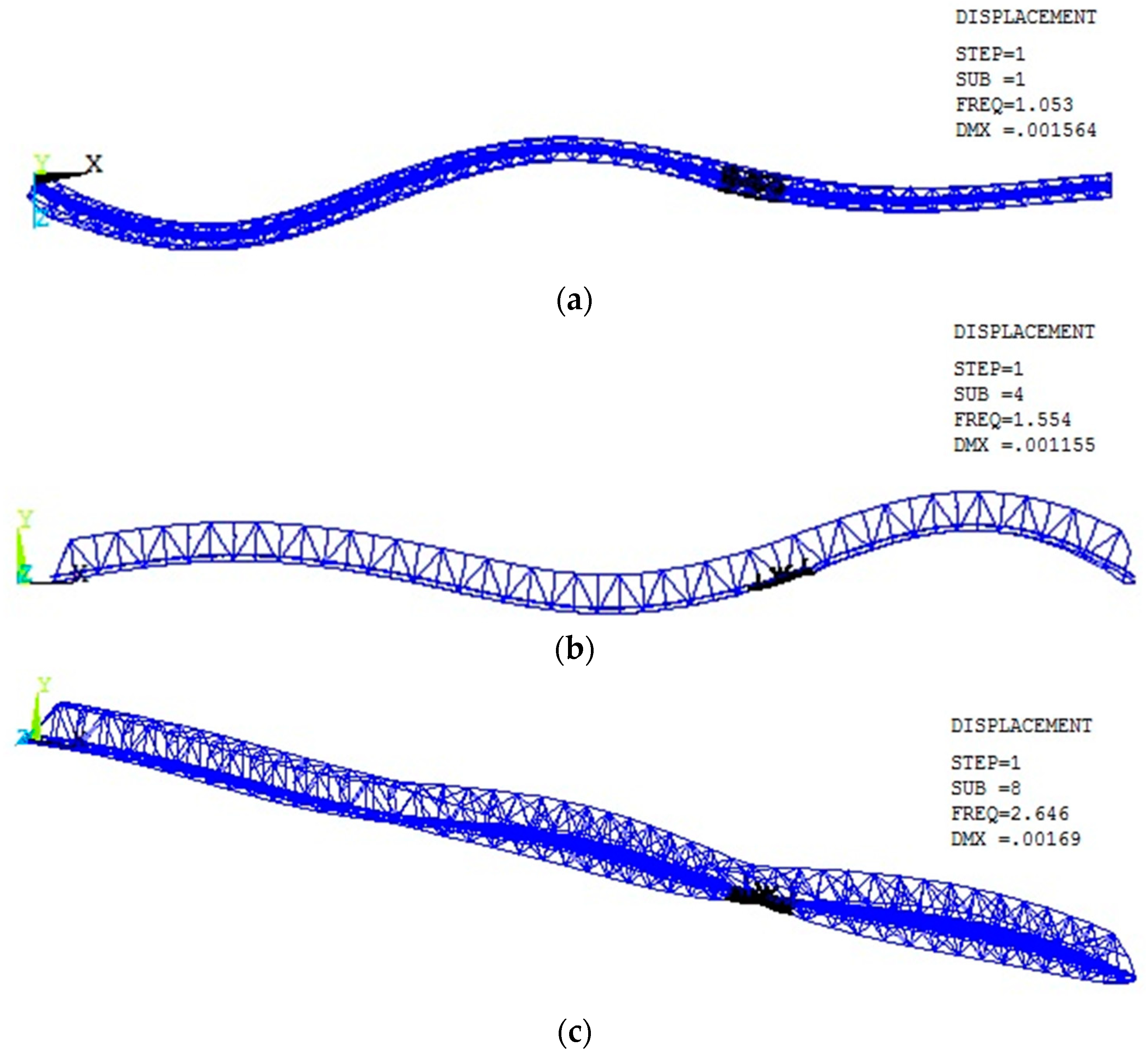
2.2. Multi-Scale FE Modeling of the Baihe Bridge
3. Multi-Scale Coupled Vibration Analysis of the TTB System
3.1. TTB System Analysis Model
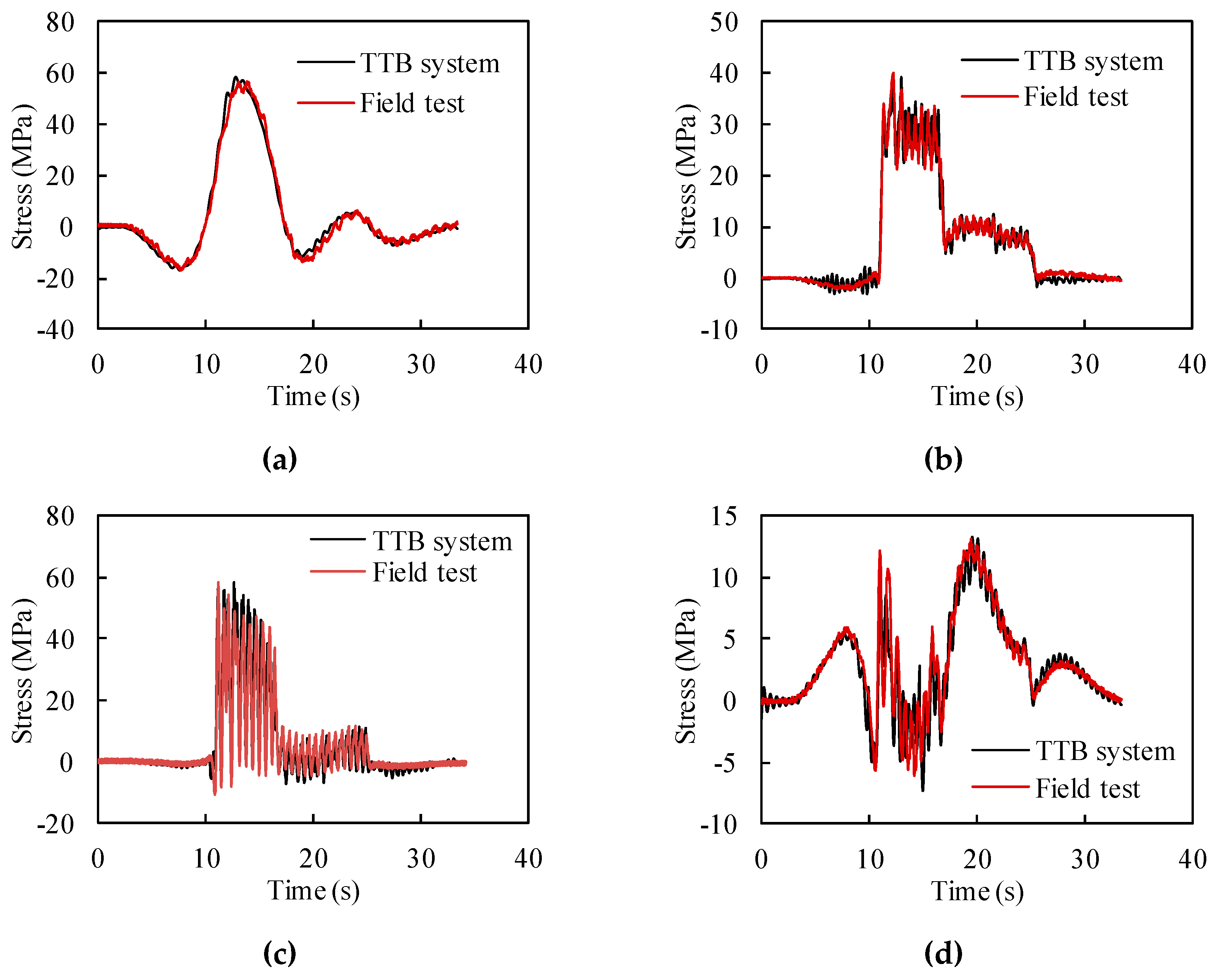
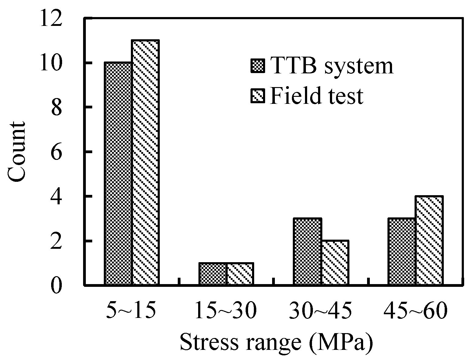
3.2. Field Test Validation
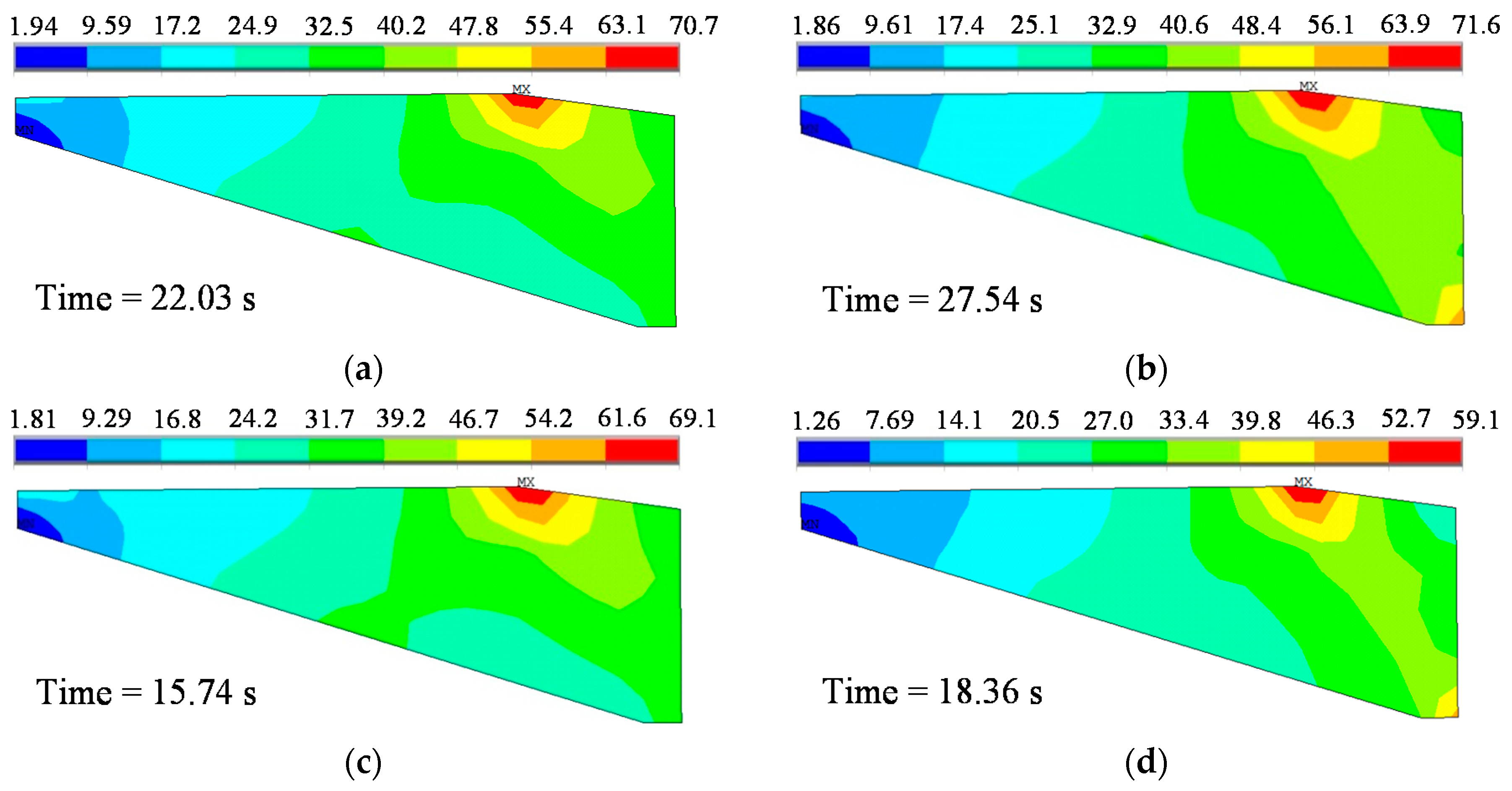
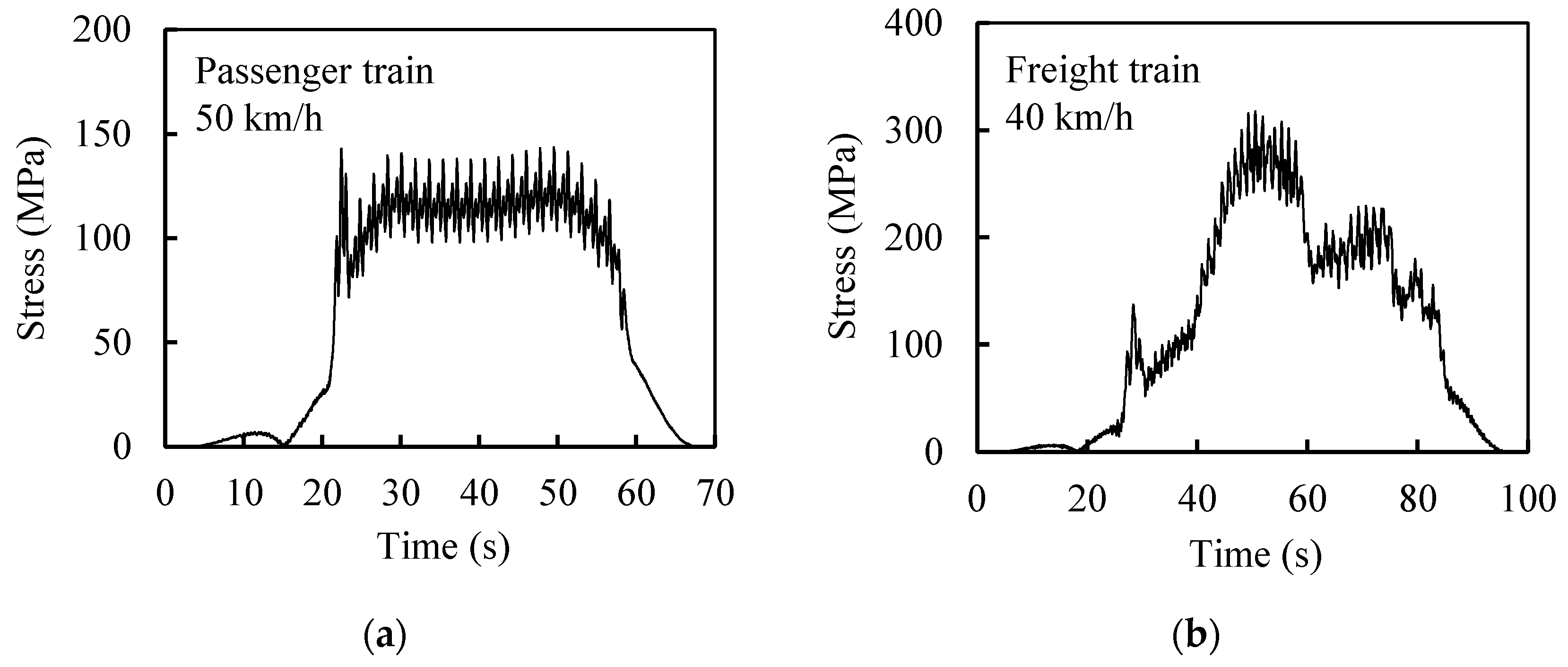
4. Fatigue Load Effects
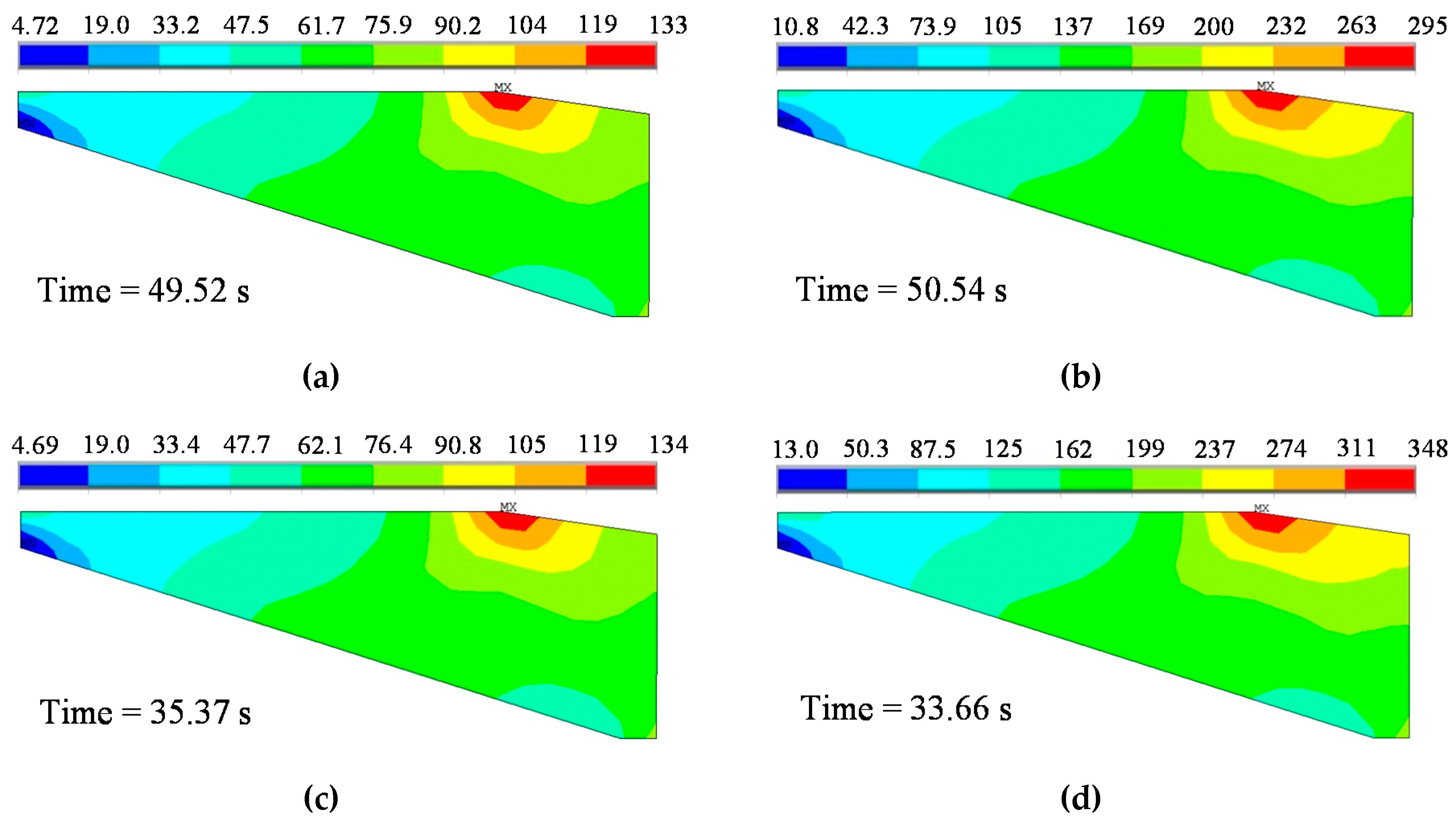
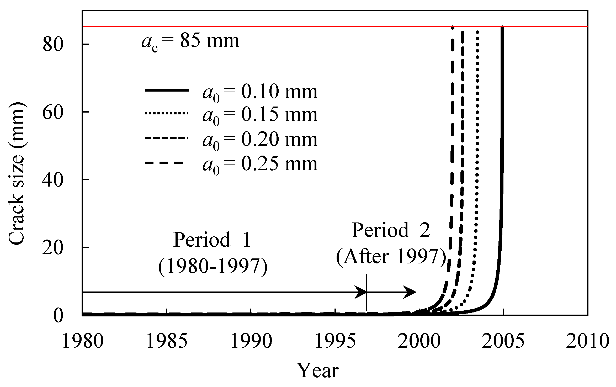
5. Fatigue Crack Propagation Analysis
5.1. Fatigue Life of the Bracket
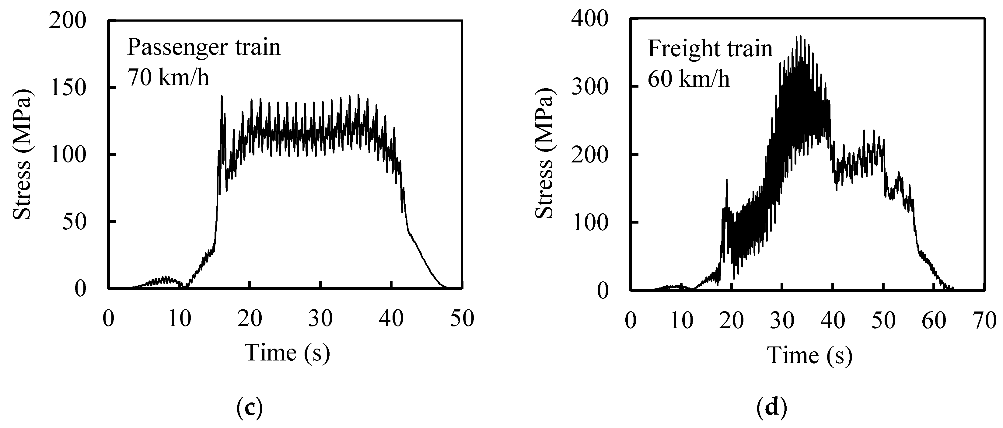
5.2. Effects of Track Irregularity and Train Speed
6. Conclusions
Author Contributions
Funding
Conflicts of Interest
References
- Deng, L.; Wang, W.; Yu, Y. State-of-the-art review on the causes and mechanisms of bridge collapse. J. Perform. Constr. Facil. 2016, 30, 04015005-1–04015005-13. [Google Scholar] [CrossRef]
- Liu, Y.; Li, D.R.; Zhang, Z.H.; Zhang, H.P.; Jiang, N. Fatigue load model using the weigh-in-motion system for highway bridges in China. J. Bridge Eng. 2017, 22, 04017011-1–04017011-8. [Google Scholar] [CrossRef]
- Siriwardane, S.; Ohga, M.; Dissanayake, R.; Taniwaki, K. Application of new damage indicator-based sequential law for remaining fatigue life estimation of railway bridges. J. Constr. Steel Res. 2008, 64, 228–237. [Google Scholar] [CrossRef]
- Basso, P.; Casciati, S.; Faravelli, L. Fatigue reliability assessment of a historic railway bridge designed by Gustave Eiffel. Struct. Infrastruct. Eng. 2015, 11, 27–37. [Google Scholar] [CrossRef]
- Liu, K.; Zhou, H.; Shi, G.; Wang, Y.Q.; Shi, Y.J.; De Roeck, G. Fatigue assessment of a composite railway bridge for high speed trains. Part II: Conditions for which a dynamic analysis is needed. J. Constr. Steel Res. 2013, 82, 246–254. [Google Scholar] [CrossRef]
- Lee, H.H.; Jeon, J.C.; Kyung, K.S. Determination of a reasonable impact factor for fatigue investigation of simple steel plate girder railway bridges. Eng. Struct. 2012, 36, 316–324. [Google Scholar] [CrossRef]
- Lippi, F.V.; Orland, M.; Salvatore, W. Assessment of the dynamic and fatigue behavior of the Panaro railway steel bridge. Struct. Infrastruct. Eng. 2013, 9, 834–848. [Google Scholar] [CrossRef]
- Zhou, H.; Liu, K.; Shi, G.; Wang, Y.Q.; Shi, Y.J.; De Roeck, G. Fatigue assessment of a composite railway bridge for high speed trains. Part I: Modeling and fatigue critical details. J. Constr. Steel Res. 2013, 82, 234–245. [Google Scholar] [CrossRef]
- Wang, F.Y.; Xu, Y.L.; Sun, B.; Zhu, Q. Dynamic stress analysis for fatigue damage prognosis of long-span bridges. Struct. Infrastruct. Eng. 2019, 15, 582–599. [Google Scholar] [CrossRef]
- Garg, V.K.; Chu, K.H.; Wiriyachai, A. Fatigue life of critical members in a railway truss bridge. Earthq. Eng. Struct. Dyn. 1982, 10, 779–795. [Google Scholar] [CrossRef]
- Leitão, F.N.; Da Silva, J.G.S.; Da SVellasco, P.C.G.; De Andrade, S.A.L.; De Lima, L.R.O. Composite (steel-concrete) highway bridge fatigue assessment. J. Constr. Steel Res. 2011, 67, 14–24. [Google Scholar] [CrossRef]
- Zhang, W.; Cai, C.S. Fatigue reliability assessment for existing bridges considering vehicle speed and road surface conditions. J. Bridge Eng. 2012, 17, 443–453. [Google Scholar] [CrossRef]
- Zhang, W.; Cai, C.S.; Pan, F. Fatigue reliability assessment for long-span bridges under combined dynamic loads from winds and vehicles. J. Bridge Eng. 2013, 18, 735–747. [Google Scholar] [CrossRef]
- Wang, W.; Deng, L.; Shao, X.D. Fatigue design of steel bridges considering the effect of dynamic vehicle loading and overloaded trucks. J. Bridge Eng. 2016, 21, 04016048-1–04016048-12. [Google Scholar] [CrossRef]
- Li, H.L.; Xia, H.; Soliman, M.; Frangopol, D.M. Bridge stress calculation based on the dynamic response of coupled train-bridge system. Eng. Struct. 2015, 99, 334–345. [Google Scholar] [CrossRef]
- Li, H.L.; Frangopol, D.M.; Soliman, M.; Xia, H. Fatigue reliability assessment of railway bridges based on probabilistic dynamic analysis of a coupled train-bridge system. J. Struct. Eng. 2016, 142, 04015158-1–04015158-16. [Google Scholar] [CrossRef]
- Li, H.L.; Soliman, M.; Frangopol, D.M.; Xia, H. Fatigue damage in railway steel bridges: Approach based on a dynamic train-bridge coupled model. J. Bridge Eng. 2017, 22, 06017006-1–06017006-8. [Google Scholar] [CrossRef]
- Zhou, H.; Shi, G.; Wang, Y.Q.; Chen, H.T.; De Roeck, G. Fatigue evaluation of a composite railway bridge based on fracture mechanics through global-local dynamic analysis. J. Constr. Steel Res. 2016, 122, 1–13. [Google Scholar] [CrossRef]
- Hou, Y.F.; Yang, Z.M.; Zhang, N. Report on the Routine Inspection of the Baihe Bridge in Jing-Tong Railway Line; Rep. No. 24; Beijing Railway Bureau: Beijing, China, 2012. (In Chinese) [Google Scholar]
- ANSYS 15. Computer Software; ANSYS: Canonsburg, PA, USA, 2013. [Google Scholar]
- Yang, Y.B.; Yau, J.D.; Wu, Y.S. Vehicle-Bridge Interaction Dynamics: With Applications to High-Speed Railways; World Scientific: Singapore, 2004. [Google Scholar]
- Xia, H.; De Roeck, G.; Goicolea, J.M. Bridge Vibration and Controls: New Research; Nova Science: New York, NY, USA, 2012. [Google Scholar]
- Zhai, W.M.; Xia, H.; Cai, C.B.; Gao, M.M.; Li, X.Z.; Guo, X.R.; Zhang, N.; Wang, K.Y. High-speed train-track-bridge dynamic interactions—Part I: Theoretical model and numerical simulation. Int. J. Rail Transp. 2013, 1, 3–24. [Google Scholar] [CrossRef]
- Zhai, W.M.; Han, Z.L.; Chen, Z.W.; Ling, L.; Zhu, S.Y. Train-track-bridge dynamic interaction: A state-of-the-art review. Veh. Syst. Dyn. 2019, 57, 984–1027. [Google Scholar] [CrossRef] [Green Version]
- Yang, S.C.; Hwang, S.H. Train-track-bridge interaction by coupling direct stiffness method and mode superposition method. J. Bridge Eng. 2016, 21, 04016058-1–04016058-16. [Google Scholar] [CrossRef]
- Li, H.L.; Xia, H. Fatigue stress analysis of a steel railway bridge using dynamic train-bridge system model. In Proceedings of the Third International Conference on Railway Technology: Research, Development and Maintenance, Cagliari, Italy, 5–8 April 2016; pp. 1–15. [Google Scholar]
- Zhai, W.M.; Wang, K.Y.; Cai, C.B. Fundamentals of vehicle-track coupled dynamics. Veh. Syst. Dyn. 2009, 47, 1349–1376. [Google Scholar] [CrossRef]
- Guo, W.W.; Xia, H.; De Roeck, G.; Liu, K. Integral model for train-track-bridge interaction on the Sesia viaduct: Dynamic simulation and critical assessment. Comput. Struct. 2012, 112–113, 205–216. [Google Scholar] [CrossRef]
- Zhang, N.; Xia, H.; Guo, W.W.; De Roeck, G. A vehicle-bridge linear interaction model and its validation. Int. J. Struct. Stab. Dyn. 2010, 10, 335–361. [Google Scholar] [CrossRef]
- MATLAB. Computer Software; MathWorks: Natick, MA, USA, 2015. [Google Scholar]
- Garg, V.K.; Dukkipati, R.V. Dynamics of Railway Vehicle System; Academic Press: Toronto, ON, Canada, 1984. [Google Scholar]
- Chen, G.; Zhai, W.M.; Zuo, H.F. Comparing track irregularities PSD of Chinese main lines with foreign typical lines by numerical simulation computation. J. China Railw. Soc. 2001, 23, 82–87. (In Chinese) [Google Scholar]
- Huang, D.Z. Dynamic analysis of steel curved box girder bridges. J. Bridge Eng. 2001, 6, 506–513. [Google Scholar] [CrossRef]
- Downing, S.D.; Socie, D.F. Simple rainflow counting algorithms. Int. J. Fatigue 1982, 4, 31–40. [Google Scholar] [CrossRef]
- Zhang, Y.L.; Xin, X.Z.; Cui, X. Updating fatigue damage coefficient in railway bridge design code in China. J. Bridge Eng. 2012, 17, 788–793. [Google Scholar] [CrossRef]
- Paris, P.; Erdogan, F. A critical analysis of crack propagation laws. J. Basic Eng. 1963, 85, 528–534. [Google Scholar] [CrossRef]
- Tada, H.; Paris, P.; Irwin, G. The Stress Analysis of Cracks Handbook; Del Research Corporation: Hellertown, PA, USA, 1973. [Google Scholar]
- Miner, M.A. Cumulative damage in fatigue. J. Appl. Mech. 1945, 12, A159–A164. [Google Scholar]
- Madsen, H.O. Random fatigue crack growth and inspection. In Proceedings of the International Conference on Structural Safety and Reliability ICOSSAR’85, Kobe, Japan, 27–29 May 1985; pp. I-475–I-484. [Google Scholar]
- British Standards Institution. Code of Practice for Fatigue Design and Assessment of Steel Structures; BS 7608: London, UK, 1993. [Google Scholar]
- Fisher, J.W. Fatigue and Fracture in Steel Bridges: Case Studies; John Willey & Sons: New York, NY, USA, 1984. [Google Scholar]


| Components | Elastic Modulus (GPa) | Density (kg/m3) | Poisson’s Ratio | Yield Strength (MPa) |
|---|---|---|---|---|
| Truss member, stringer, floor beam, and bracing | 206 | 7850 | 0.30 | 345 |
| Some truss chords, gusset, and connection | 206 | 7850 | 0.30 | 420 |
| Steel rail | 206 | 7850 | 0.30 | 630 |
| Wooden sleeper | 9 | 600 | 0.43 | N/A |
| Track Class | Parameter | Allowed Speed (km/h) | ||||
|---|---|---|---|---|---|---|
| Aa (cm2 rad/m) | Av (cm2 rad/m) | Ωc (rad/m) | Ωs (rad/m) | Passenger Train | Freight Train | |
| 1 | 3.3634 | 1.2107 | 0.8245 | 0.6046 | 24 | 16 |
| 2 | 1.2107 | 1.0181 | 0.8245 | 0.9308 | 48 | 40 |
| 3 | 0.4128 | 0.6816 | 0.8245 | 0.8520 | 96 | 64 |
| 4 | 0.3027 | 0.5376 | 0.8245 | 1.1312 | 128 | 96 |
| 5 | 0.0762 | 0.2095 | 0.8245 | 0.8209 | 144 | 128 |
| 6 | 0.0339 | 0.0339 | 0.8245 | 0.4380 | 176 | 176 |
| Parameter | Unit | Locomotive | Wagon |
|---|---|---|---|
| Mass of the car-body | kg | 9.05e4 | 1.56e4 |
| Moment of inertia of car-body around longitudinal axis | kg m2 | 8.88e4 | 2.66e4 |
| Moment of inertia of car-body around lateral axis | kg m2 | 2.88e6 | 2.66e5 |
| Moment of inertia of car-body around vertical axis | kg m2 | 2.88e6 | 2.84e5 |
| Mass of the bogie | kg | 1.02e4 | 1.13e3 |
| Moment of inertia of bogie around longitudinal axis | kg m2 | 5e3 | 1.92e2 |
| Moment of inertia of bogie around lateral axis | kg m2 | 2.26e4 | 4.19e2 |
| Moment of inertia of bogie around vertical axis | kg m2 | 2.26e4 | 4.19e2 |
| Mass of the wheelset | kg | 4.52e3 | 1.2e3 |
| Moment of inertia of wheelset around longitudinal axis | kg m2 | 3.26e4 | 7.4e2 |
| Moment of inertia of wheelset around vertical axis | kg m2 | 3.26e4 | 7.4e2 |
| Primary vertical spring stiffness | N/m | 1.47e6 | 1.7e7 |
| Primary lateral spring stiffness | N/m | 2.65e6 | 3.6e6 |
| Primary longitudinal spring stiffness | N/m | 0 | 3.6e6 |
| Secondary vertical spring stiffness | N/m | 6.62e6 | 5.32e6 |
| Secondary lateral spring stiffness | N/m | 5.5e7 | 4.14e6 |
| Secondary longitudinal spring stiffness | N/m | 0 | 6.5e6 |
| Primary vertical damping | N s/m | 1.2e5 | 3e3 |
| Primary lateral damping | N s/m | 0 | 0 |
| Primary longitudinal damping | N s/m | 0 | 0 |
| Secondary vertical damping | N s/m | 7.2e4 | 3e3 |
| Secondary lateral damping | N s/m | 1e5 | 0 |
| Secondary longitudinal damping | N s/m | 0 | 0 |
| Half span of the primary suspension system | m | 1.025 | 1 |
| Half span of the secondary suspension system | m | 1.025 | 1 |
| Half distance between two wheelsets | m | 1.8 | 0.875 |
| Half distance between two bogies | m | 6.0 | 4.35 |
| Half distance between two car-body couplers | m | 21.1 | 13.438 |
| Wheel radius | m | 0.525 | 0.42 |
| Distance between the car-body and the secondary suspension system | m | 1.744 | 0.74 |
| Distance between the secondary suspension system and bogie | m | 0.010 | 0.59 |
| Distance between the bogie and wheelsets | m | 0.55 | 0.015 |
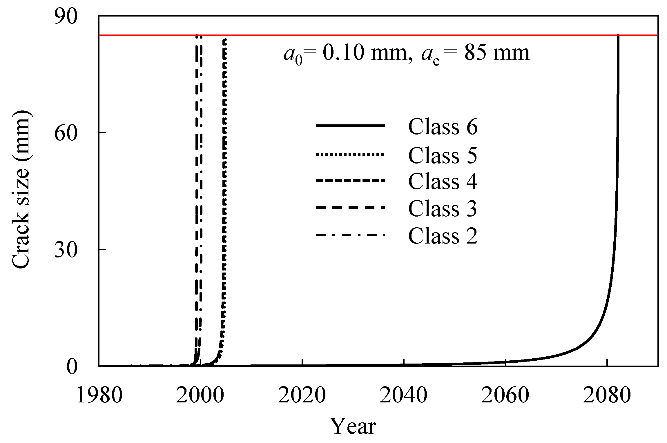
| Track Irregularity Class | ΔSeq (MPa) in Equation (12) | ∑ni in Equation (12) | Time of the Crack Size Reaching 85 mm | ||
|---|---|---|---|---|---|
| 1980–1997 | After 1997 | 1980–1997 | After 1997 | a0 = 0.1 mm, ac = 85 mm | |
| 2 | 18.55 | 44.87 | 69810 | 43128 | 2000 |
| 3 | 11.25 | 70.28 | 61440 | 34140 | 1999 |
| 4 | 13.75 | 39.19 | 57702 | 34574 | 2004 |
| 5 | 11.45 | 41.40 | 48804 | 30584 | 2004 |
| 6 | 9.09 | 18.97 | 43770 | 27486 | 2082 |
| Track Irregularities | Vertical Wheel-Rail Force (kN) | Lateral Wheel-Rail Force (kN) | Torsional Wheel-Rail Moment (kN m) |
|---|---|---|---|
| Class 2 | 267.5 | 46.9 | 56.7 |
| Class 3 | 250.1 | 23.3 | 48.1 |
| Class 4 | 243.2 | 23.0 | 38.5 |
| Class 5 | 238.3 | 10.7 | 29.1 |
| Class 6 | 229.1 | 5.88 | 9.98 |
| No irregularities | 226.9 | 2.54 | 5.83 |
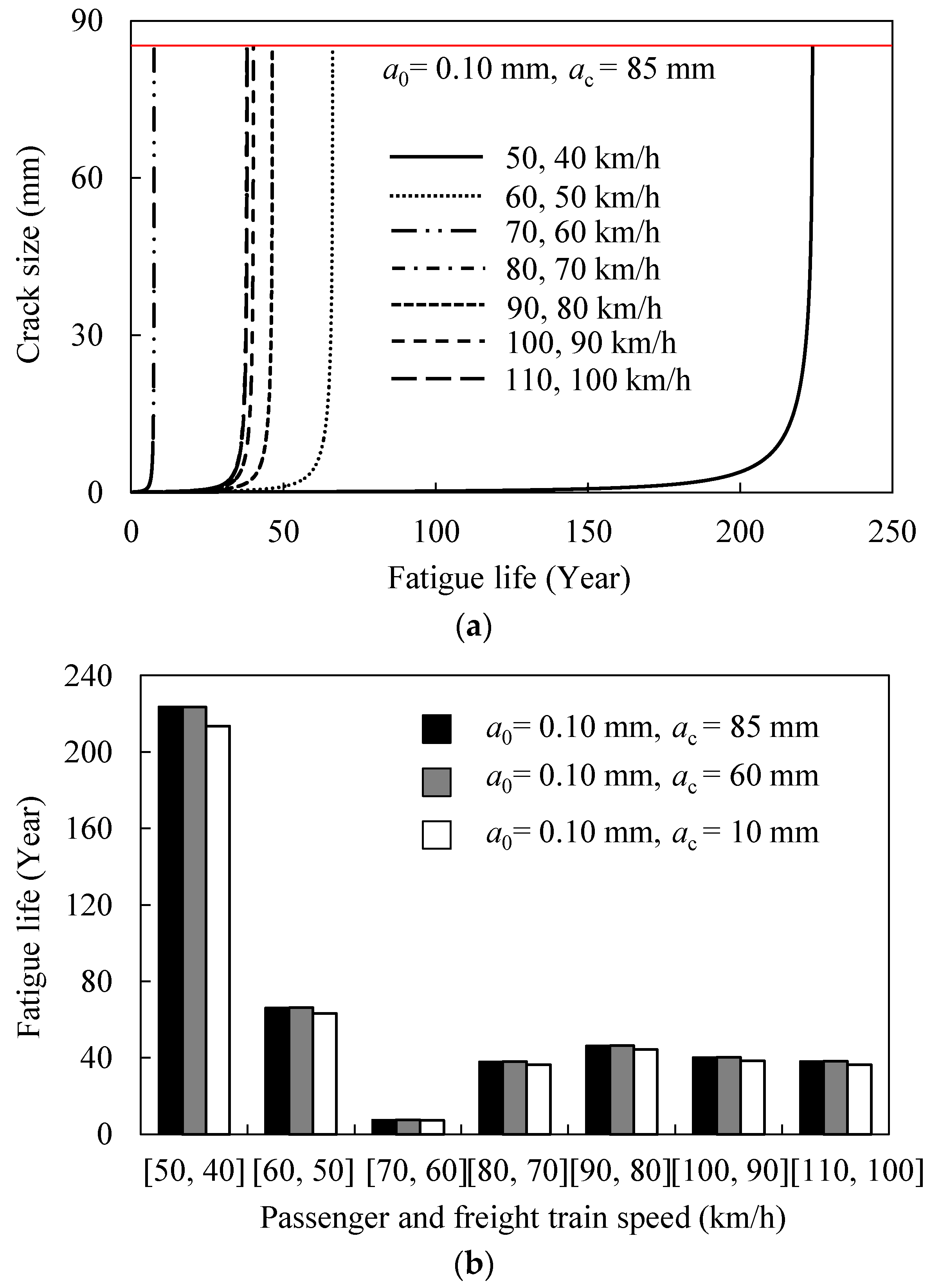
| Operating Speed (km/h) | ΔSeq (MPa) in Equation (12) | ∑ni in Equation (12) | Fatigue Life N in Terms of Stress Cycle Number | |||
|---|---|---|---|---|---|---|
| Passenger Train | Freight Train | a0 = 0.1 mm ac = 85 mm | a0 = 0.1 mm ac = 60 mm | a0 = 0.1 mm ac = 10 mm | ||
| 50 | 40 | 11.45 | 48804 | 3.9858e9 | 3.9821e9 | 3.8042e9 |
| 60 | 50 | 19.27 | 34602 | 8.3577e8 | 8.3499e8 | 7.9769e8 |
| 70 | 60 | 41.40 | 30584 | 8.4321e7 | 8.4242e7 | 8.0479e7 |
| 80 | 70 | 23.53 | 33160 | 4.5923e8 | 4.5880e8 | 4.3830e8 |
| 90 | 80 | 23.44 | 27460 | 4.6488e8 | 4.6445e8 | 4.4370e8 |
| 100 | 90 | 24.31 | 28418 | 4.1650e8 | 4.1612e8 | 3.9753e8 |
| 110 | 100 | 26.40 | 23382 | 3.2518e8 | 3.2488e8 | 3.1036e8 |
© 2020 by the authors. Licensee MDPI, Basel, Switzerland. This article is an open access article distributed under the terms and conditions of the Creative Commons Attribution (CC BY) license (http://creativecommons.org/licenses/by/4.0/).
Share and Cite
Li, H.; Wu, G. Fatigue Evaluation of Steel Bridge Details Integrating Multi-Scale Dynamic Analysis of Coupled Train-Track-Bridge System and Fracture Mechanics. Appl. Sci. 2020, 10, 3261. https://0-doi-org.brum.beds.ac.uk/10.3390/app10093261
Li H, Wu G. Fatigue Evaluation of Steel Bridge Details Integrating Multi-Scale Dynamic Analysis of Coupled Train-Track-Bridge System and Fracture Mechanics. Applied Sciences. 2020; 10(9):3261. https://0-doi-org.brum.beds.ac.uk/10.3390/app10093261
Chicago/Turabian StyleLi, Huile, and Gang Wu. 2020. "Fatigue Evaluation of Steel Bridge Details Integrating Multi-Scale Dynamic Analysis of Coupled Train-Track-Bridge System and Fracture Mechanics" Applied Sciences 10, no. 9: 3261. https://0-doi-org.brum.beds.ac.uk/10.3390/app10093261