Author Contributions
Conceptualization, H.I. and M.R.K.; Data curation, M.S.F.b.M.; Formal analysis, H.I. and A.F.b.A.; Funding acquisition, M.R.K.; Investigation, A.F.b.A.; Methodology, H.I. and M.R.K.; Project administration, M.R.K. and A.F.b.A.; software, H.I.; supervision, M.R.K.; Validation, H.I.; Visualization, A.F.b.A.; Writing—original draft, H.I. and M.S.F.b.M.; Writing—review & editing, M.R.K. and A.F.b.A. All authors have read and agreed to the published version of the manuscript.
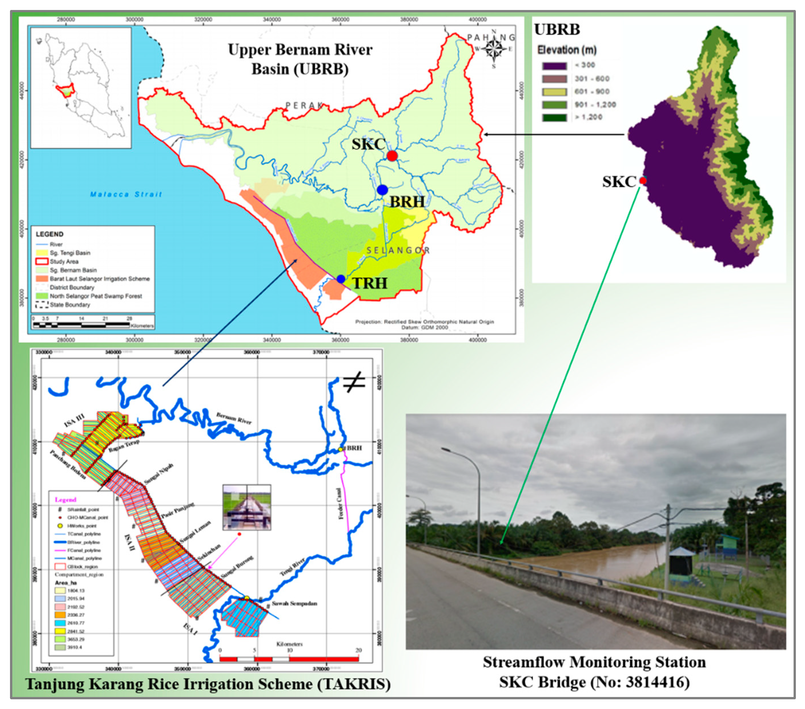
Figure 1.
Map of the Tanjung Karang Rice Irrigation Scheme [
26].
Figure 1.
Map of the Tanjung Karang Rice Irrigation Scheme [
26].
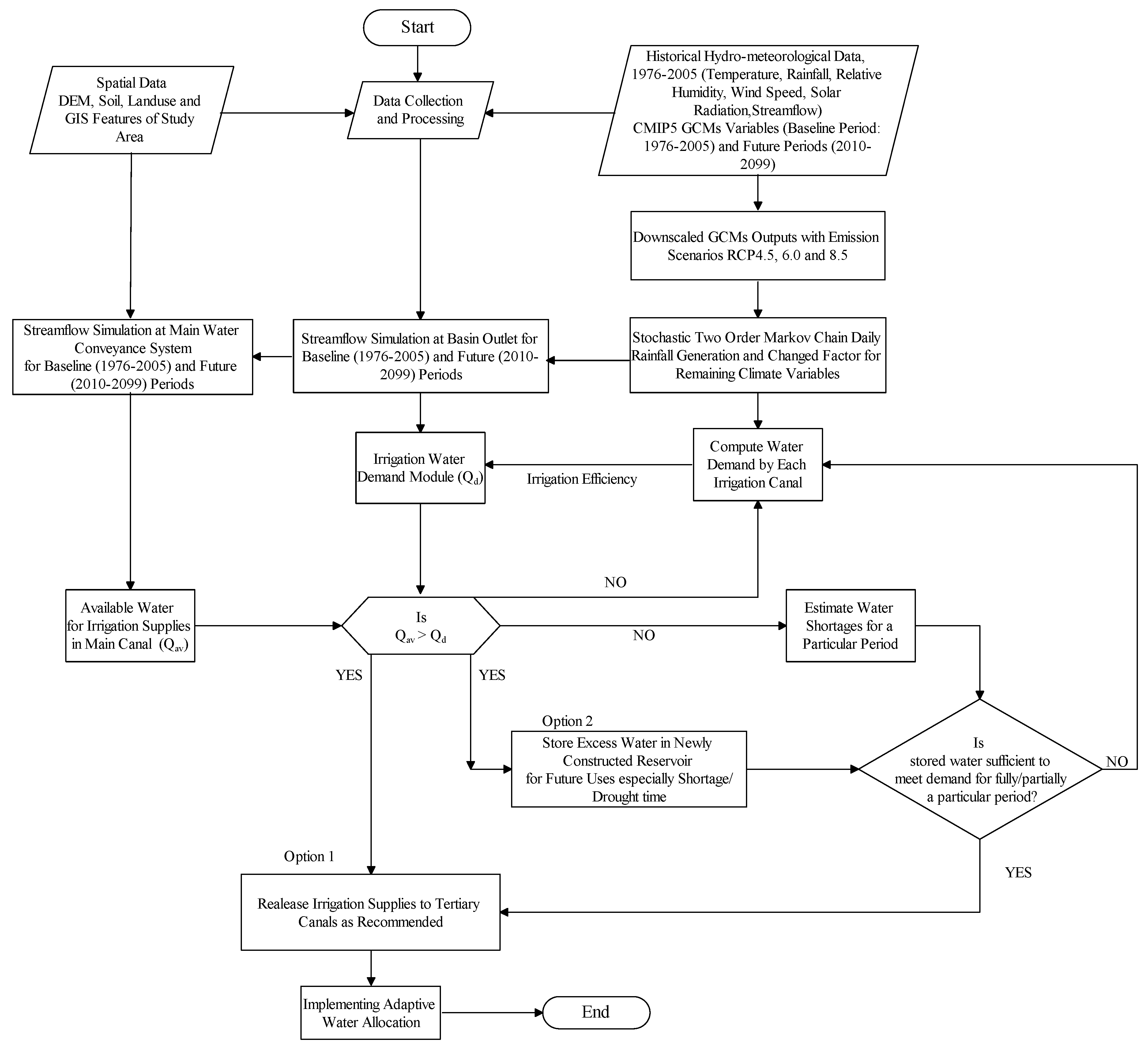
Figure 2.
Framework for the development of the climate-smart agro-hydrological model.
Figure 2.
Framework for the development of the climate-smart agro-hydrological model.
Figure 3.
Projected average monthly effective rainfall using multiple models under RCPs 4.5, 6.0, and 8.5 for the periods 2010–2039, 2040–2069, and 2070–2099 with respect to the 1976–2005 baseline.
Figure 3.
Projected average monthly effective rainfall using multiple models under RCPs 4.5, 6.0, and 8.5 for the periods 2010–2039, 2040–2069, and 2070–2099 with respect to the 1976–2005 baseline.
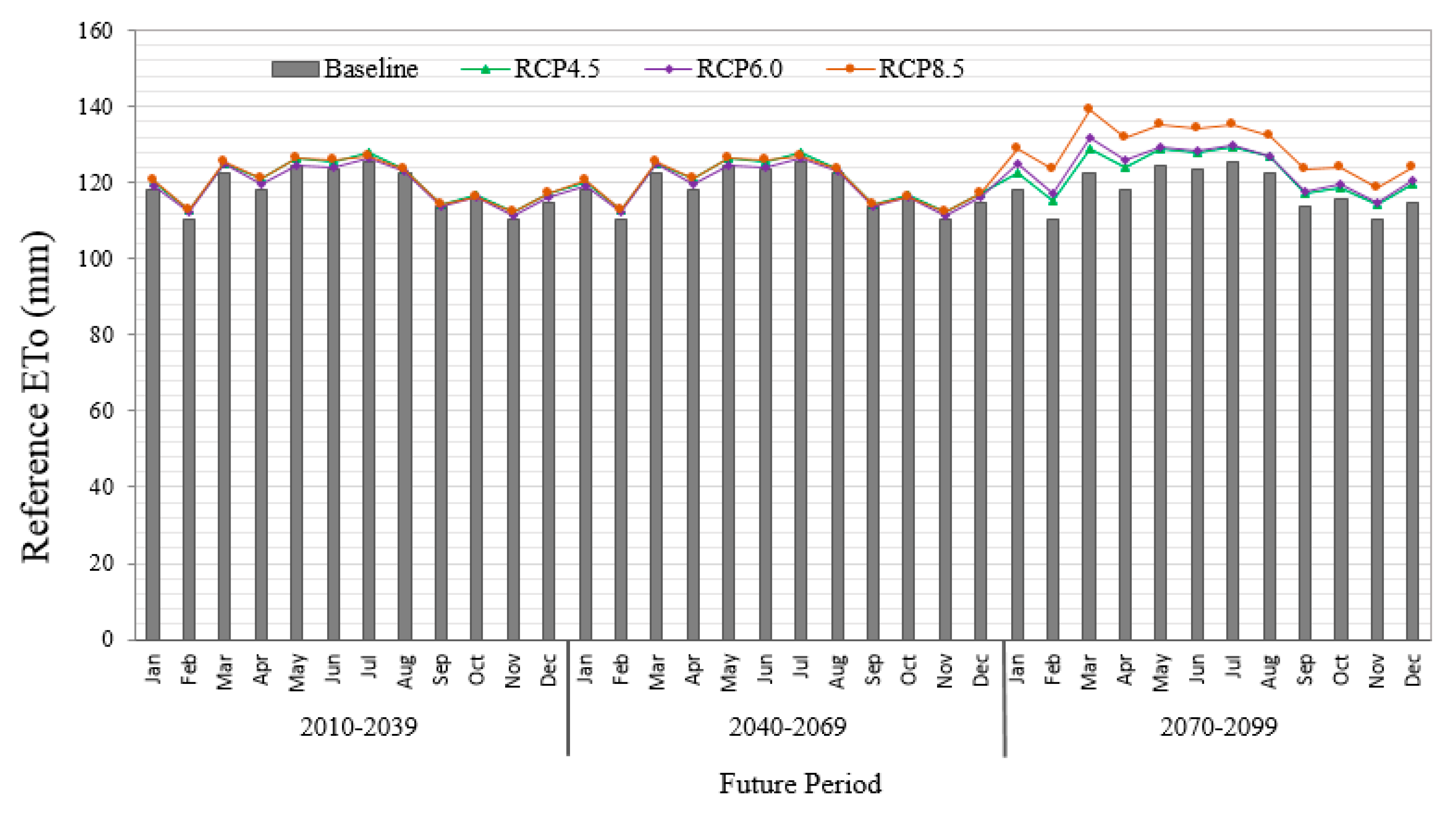
Figure 4.
Projected mean monthly ensemble of multi-model reference evapotranspiration (ET0) for RCP4.5, RCP6.0, and RCP8.5 scenarios and future periods of 2020s, 2050s, and 2080s compared to the baseline period.
Figure 4.
Projected mean monthly ensemble of multi-model reference evapotranspiration (ET0) for RCP4.5, RCP6.0, and RCP8.5 scenarios and future periods of 2020s, 2050s, and 2080s compared to the baseline period.
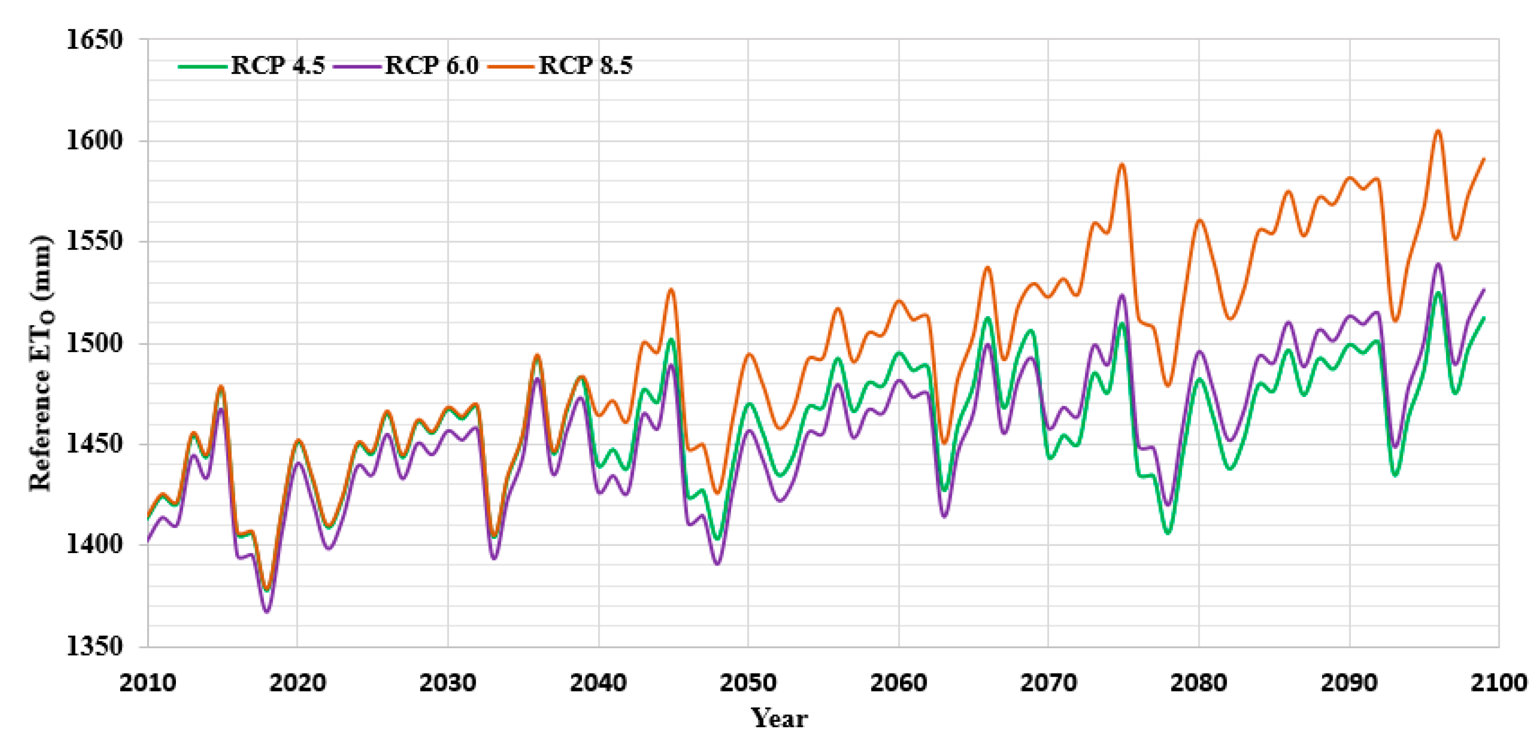
Figure 5.
Projected multi-model annual reference evapotranspiration (ET0) for the RCP4.5, RCP6.0, and RCP8.5 scenarios from 2010 to 2099.
Figure 5.
Projected multi-model annual reference evapotranspiration (ET0) for the RCP4.5, RCP6.0, and RCP8.5 scenarios from 2010 to 2099.
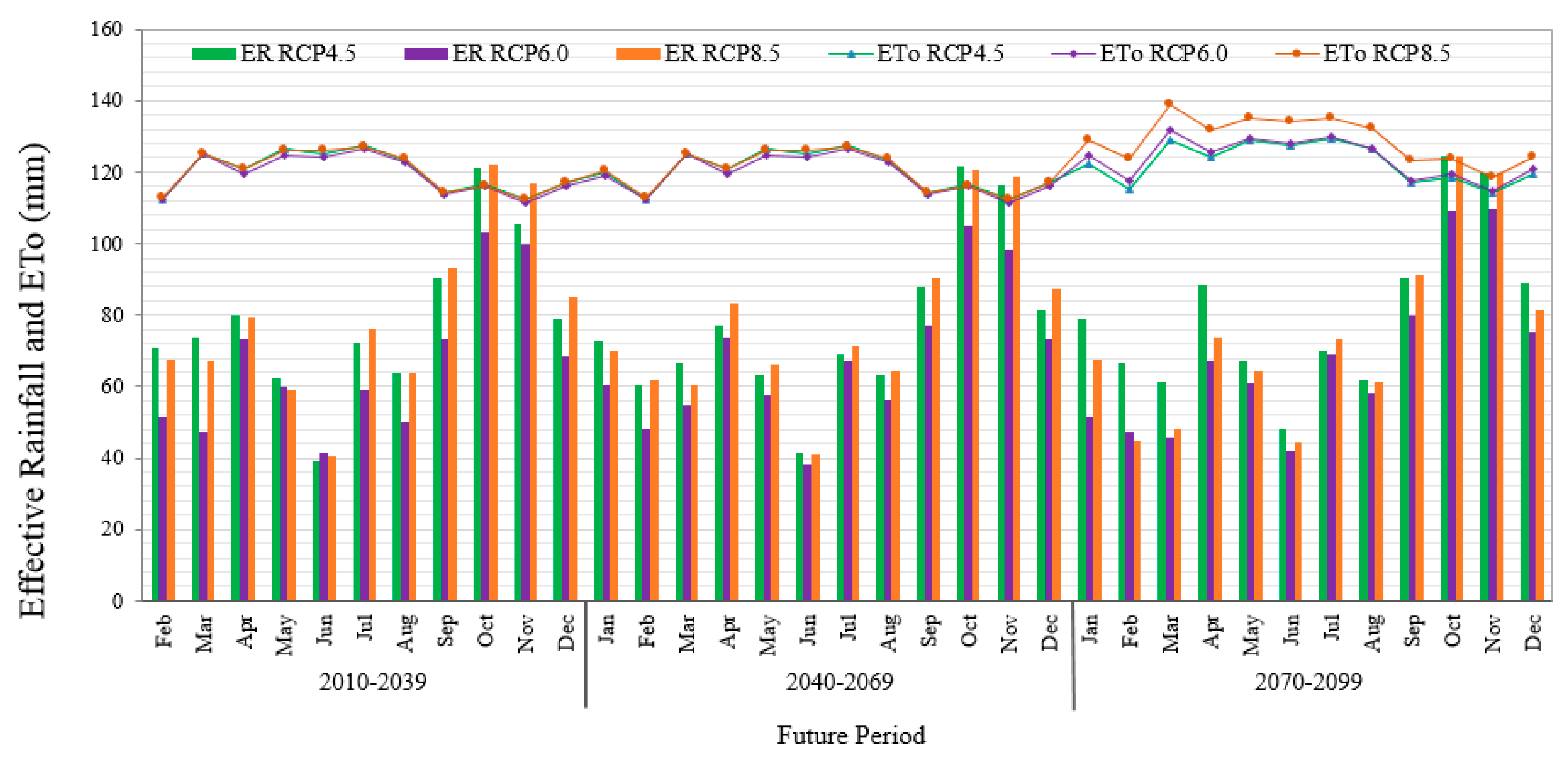
Figure 6.
Projected monthly multi-model effective rainfall (ER) and reference evapotranspiration (ET0) for RCP scenarios in future periods (2010–2099).
Figure 6.
Projected monthly multi-model effective rainfall (ER) and reference evapotranspiration (ET0) for RCP scenarios in future periods (2010–2099).
Figure 7.
Projected mean monthly streamflow from multiple models for three RCP scenarios (RCPs 4.5, 6.0, and 8.5) for three future periods of 2010–2039, 2040–2069, and 2070–2099 relative to the baseline period of 1976–2005.
Figure 7.
Projected mean monthly streamflow from multiple models for three RCP scenarios (RCPs 4.5, 6.0, and 8.5) for three future periods of 2010–2039, 2040–2069, and 2070–2099 relative to the baseline period of 1976–2005.
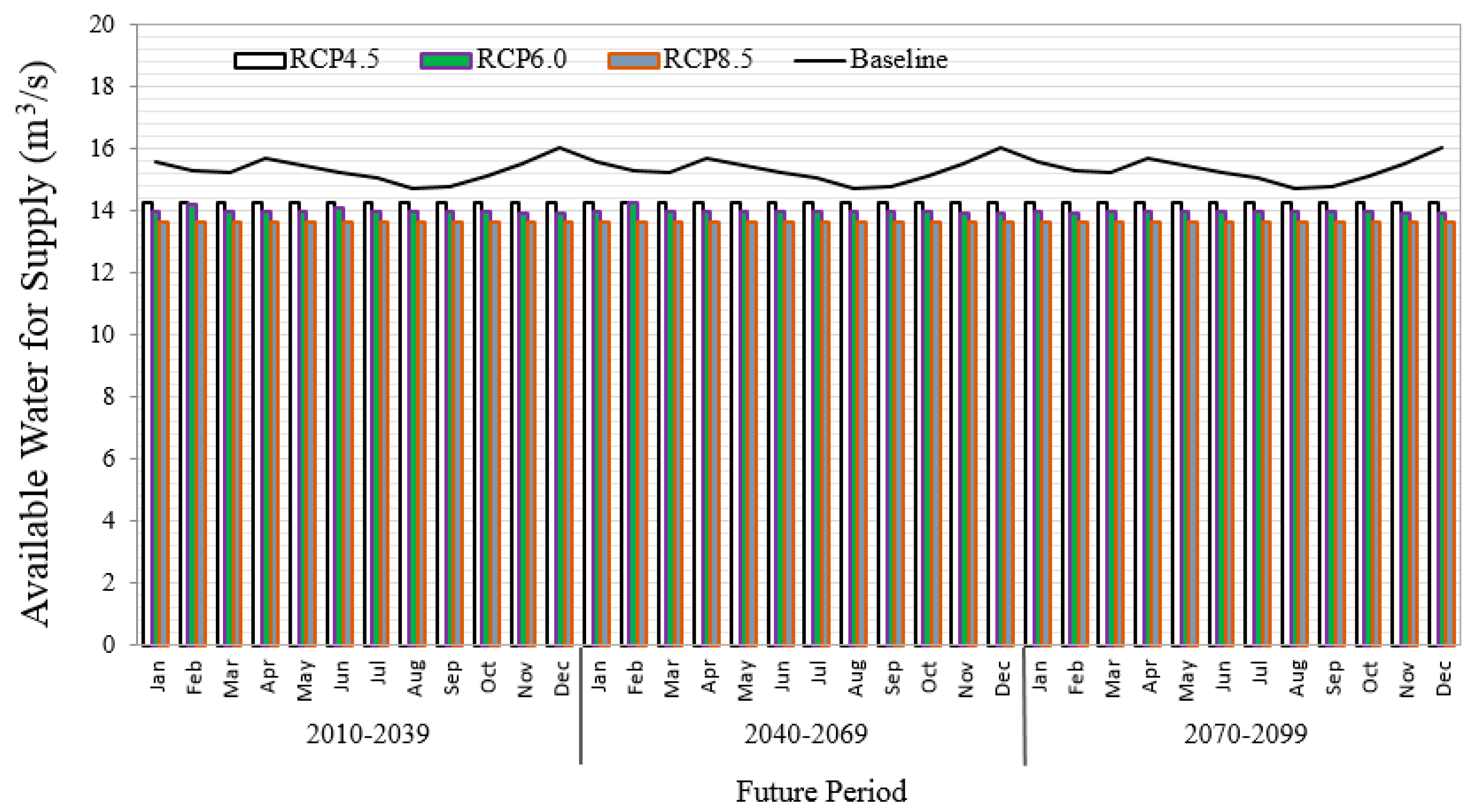
Figure 8.
Projected mean monthly available supply from multiple models for three RCP scenarios (RCPs 4.5, 6.0, and 8.5) for three future periods of 2010–2039, 2040–2069, and 2070–2099 relative to the baseline period of 1976–2005.
Figure 8.
Projected mean monthly available supply from multiple models for three RCP scenarios (RCPs 4.5, 6.0, and 8.5) for three future periods of 2010–2039, 2040–2069, and 2070–2099 relative to the baseline period of 1976–2005.
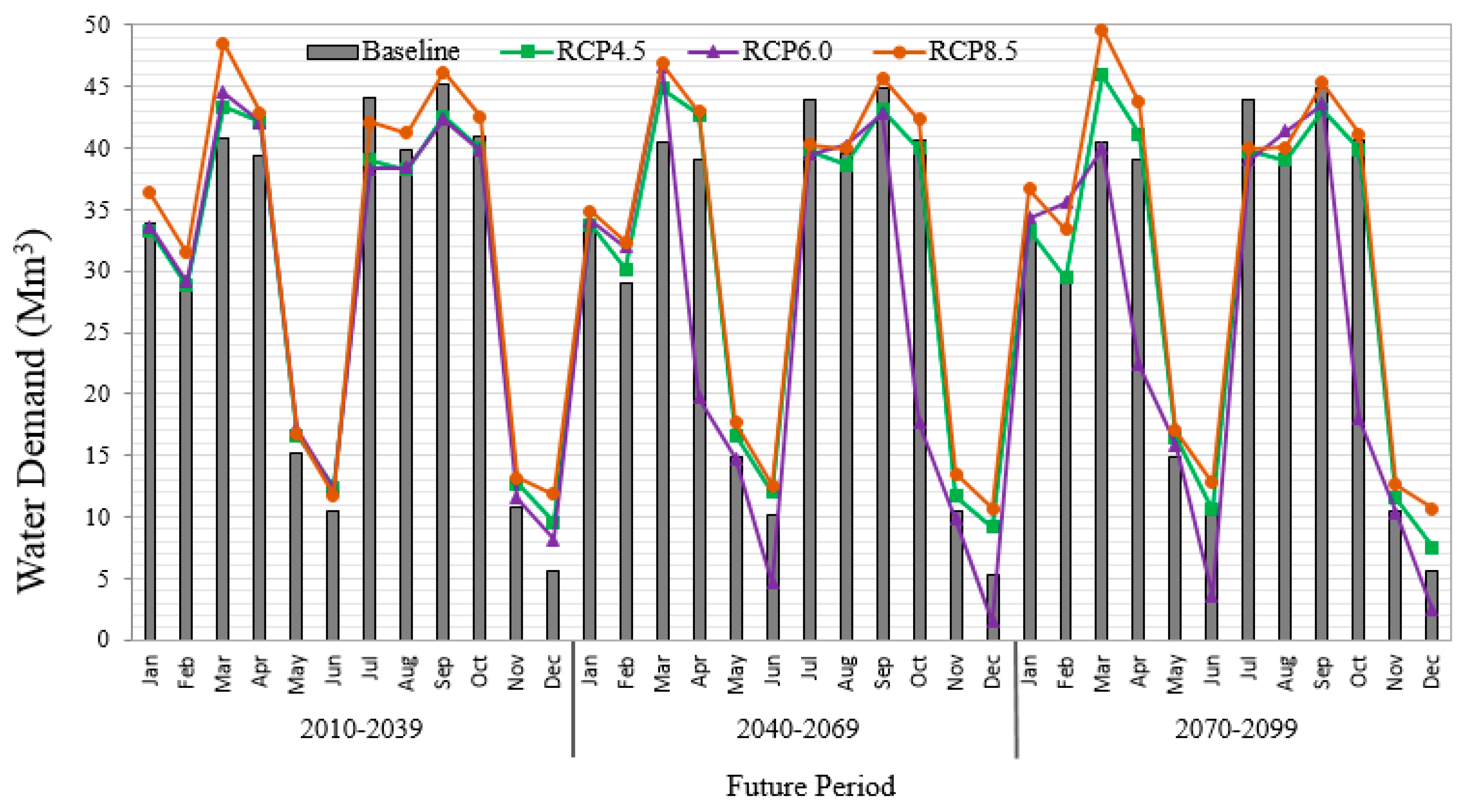
Figure 9.
Projected mean monthly water demand from multiple models for three RCP scenarios (RCPs 4.5, 6.0, and 8.5) for three future periods of 2010–2039, 2040–2069, and 2070–2099 relative to the baseline period of 1976–2005.
Figure 9.
Projected mean monthly water demand from multiple models for three RCP scenarios (RCPs 4.5, 6.0, and 8.5) for three future periods of 2010–2039, 2040–2069, and 2070–2099 relative to the baseline period of 1976–2005.
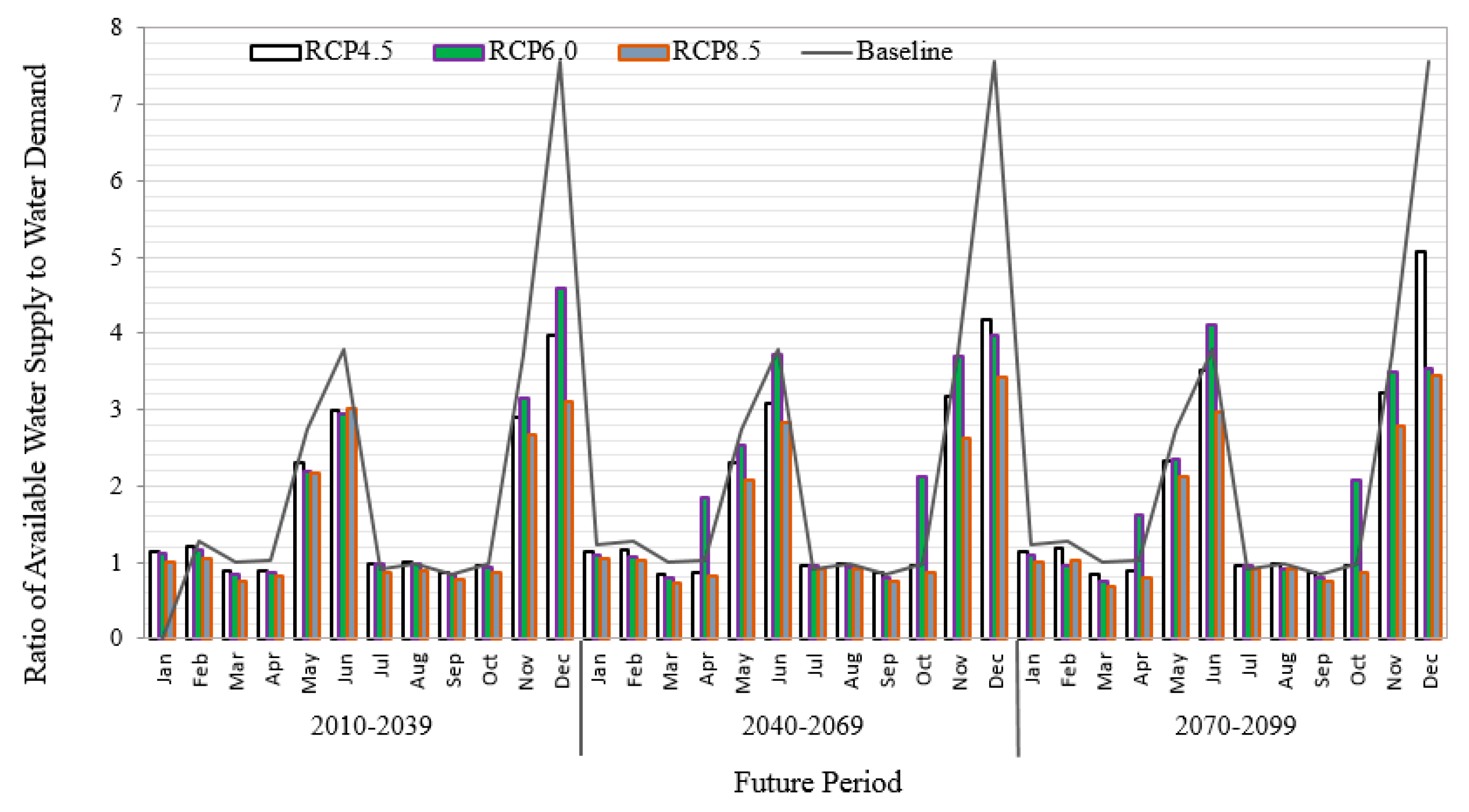
Figure 10.
Projected ratio of available water for supply (WS) to water demand (WD) from multiple models for three RCP scenarios (RCPs 4.5, 6.0, and 8.5) for three future periods of 2010–2039, 2040–2069, and 2070–2099 relative to the baseline period of 1976–2005.
Figure 10.
Projected ratio of available water for supply (WS) to water demand (WD) from multiple models for three RCP scenarios (RCPs 4.5, 6.0, and 8.5) for three future periods of 2010–2039, 2040–2069, and 2070–2099 relative to the baseline period of 1976–2005.
Table 1.
Current cropping calendar and distribution of irrigation supplies for the dry and wet irrigation seasons in the Tanjung Karang Rice Irrigation Scheme.
Table 1.
Current cropping calendar and distribution of irrigation supplies for the dry and wet irrigation seasons in the Tanjung Karang Rice Irrigation Scheme.
| Cropping Activities | Dry Season | Wet Season |
|---|
| | ISA I | ISA II | ISA III | ISA IV | ISA I | ISA II | ISA III | ISA IV |
|---|
| Pre-saturation | 1-January | 1-February | 1-March | 1-April | 1-July | 1-August | 1-September | 1-October |
| Sowing starts | 15-January | 15-February | 15-March | 15-April | 15-July | 15-August | 15-September | 15-October |
| Normal irrigation | 1-February | 1-March | 1-April | 1-May | 1-August | 1-September | 1-October | 1-November |
| Irrigation ends | 10-April | 10-May | 10-June | 10-July | 10-October | 10-November | 10-December | 10-January |
Table 2.
Projected annual changes in effective rainfall (%) by global climate models (GCMs) under Representative Concentration Pathways (RCPs) 4.5, 6.0, and 8.5 for the periods 2010–2039, 2040–2069, and 2070–2099 relative to the 1976–2005 baseline period.
Table 2.
Projected annual changes in effective rainfall (%) by global climate models (GCMs) under Representative Concentration Pathways (RCPs) 4.5, 6.0, and 8.5 for the periods 2010–2039, 2040–2069, and 2070–2099 relative to the 1976–2005 baseline period.
| GCMs | RCP4.5 | RCP6.0 | RCP8.5 |
|---|
| | 2020s | 2050s | 2080s | 2020s | 2050s | 2080s | 2020s | 2050s | 2080s |
|---|
| CANESM2 | – | – | – | – | – | – | 16.38 | 27.72 | 37.85 |
| CCSM4 | −0.98 | 3.86 | 3.95 | −6.46 | −2.97 | 0.59 | −2.28 | 5.46 | −3.65 |
| CNRM | −6.58 | −0.95 | −4.47 | – | – | – | −1.88 | −7.05 | 0.00 |
| CSIRO | −1.87 | 1.33 | 8.07 | −4.65 | −9.70 | −7.14 | 0.29 | −33.5 | −72.20 |
| GFDL-ESM2G | 3.35 | 6.14 | 3.55 | 4.68 | 6.62 | 8.09 | 1.24 | 14.60 | 0.00 |
| GFDL-ESM2M | 5.56 | 2.92 | 6.47 | 7.23 | 14.46 | 14.16 | 11.72 | 5.15 | 9.28 |
| HadGEM2-CC | 13.75 | −5.13 | 5.46 | – | – | – | 4.09 | −1.47 | 0.14 |
| HadGEM2-ES | 1.97 | −9.42 | −0.65 | −55.31 | −55.46 | −62.29 | −0.78 | −8.44 | −8.23 |
| MPI-ESM-LR | 34.1 | 28.7 | 43.6 | – | – | – | 44.9 | 34.7 | 27.3 |
| MRI-CGCM3 | 2.72 | −2.88 | 10.14 | −5.43 | −0.16 | −6.08 | −3.17 | 3.85 | −5.14 |
Table 3.
Projected changes in temperature under multi-model projections based on RCP scenarios relative to the baseline period of 1976–2005.
Table 3.
Projected changes in temperature under multi-model projections based on RCP scenarios relative to the baseline period of 1976–2005.
| Period | Changes in Temperature under RCPs |
|---|
| | RCP4.5 | RCP6.0 | RCP8.5 |
|---|
| Maximum temperature (°C) | | | |
| 2020s | 0.68 | 0.52 | 0.82 |
| 2050s | 1.29 | 1.06 | 1.85 |
| 2080s | 1.57 | 1.85 | 3.25 |
| Average | 1.18 | 1.14 | 1.97 |
| Minimum temperature (°C) | | | |
| 2020s | 0.71 | 0.62 | 0.92 |
| 2050s | 1.36 | 1.16 | 1.95 |
| 2080s | 1.75 | 1.85 | 3.36 |
| Average | 1.27 | 1.21 | 2.08 |
Table 4.
Projected changes in streamflow under multi-model projections based on RCP scenarios relative to the baseline period of 1976–2005.
Table 4.
Projected changes in streamflow under multi-model projections based on RCP scenarios relative to the baseline period of 1976–2005.
| Irrigation Season | Period | Changes (%) in Streamflow |
|---|
| | RCP4.5 | RCP6.0 | RCP8.5 |
|---|
| | 2020s | −0.40 | −1.70 | −5.66 |
| Dry Season | 2050s | −0.63 | −1.90 | −5.54 |
| | 2080s | −0.18 | −1.44 | −5.94 |
| | Average | −0.40 | −1.68 | −5.71 |
| | 2020s | 0.19 | −0.84 | −3.92 |
| Wet Season | 2050s | 0.59 | −0.47 | −3.67 |
| | 2080s | 0.31 | −0.71 | −3.90 |
| | Average | 0.36 | −0.67 | −3.83 |
Table 5.
Projected annual changes in water demand under multi-model projections based on RCP scenarios.
Table 5.
Projected annual changes in water demand under multi-model projections based on RCP scenarios.
| Irrigation Season | Period | Annual Changes (%) in Water Demand under RCPs |
|---|
| | RCP4.5 | RCP6.0 | RCP8.5 |
|---|
| | 2020s | 4.36 | 5.54 | 10.03 |
| | 2050s | 6.21 | −11.40 | 11.02 |
| Dry Season | 2080s | 6.21 | −11.40 | 11.09 |
| | Average | 5.59 | −5.75 | 10.71 |
| | 2020s | −2.3 | −4.5 | −5.4 |
| Wet Season | 2050s | −2.4 | 17.5 | −5.9 |
| | 2080s | −3.3 | 14.0 | −7.3 |
| | Average | −2.6 | 9.0 | −6.2 |
Table 6.
Historical and projected water supply excess/shortage under RCP scenarios 4.5, 6.0, and 8.5 for the periods 2010–2039, 2040–2069, and 2070–2099.
Table 6.
Historical and projected water supply excess/shortage under RCP scenarios 4.5, 6.0, and 8.5 for the periods 2010–2039, 2040–2069, and 2070–2099.
| Season | Historical | | RCP4.5 | | RCP6.0 | RCP8.5 |
|---|
| | 1976–2005 | 2020s | 2050s | 2080s | 2020s | 2050s | 2080s | 2020s | 2050s | 2080s |
|---|
| Dry season | | | | | | | | | | |
| Jan | 2.92 | 1.80 | 1.65 | 1.78 | 1.38 | 1.26 | 1.16 | 0.11 | 0.67 | −0.11 |
| Feb | 3.35 | 2.46 | 1.92 | 2.19 | 2.01 | 0.89 | −0.61 | 0.76 | 0.42 | 0.20 |
| Mar | −0.03 | −1.94 | −2.47 | −2.87 | −2.66 | −3.50 | −4.61 | −4.46 | −4.94 | −6.52 |
| Apr | 0.51 | −1.98 | −2.23 | −1.61 | −2.27 | 6.38 | 5.33 | −2.87 | −2.90 | −3.53 |
| May | 9.84 | 8.06 | 8.07 | 8.14 | 7.56 | 8.44 | 8.04 | 7.37 | 7.10 | 7.22 |
| June | 11.21 | 9.50 | 9.65 | 10.20 | 9.23 | 12.22 | 12.57 | 9.12 | 8.83 | 9.07 |
| Wet season | | | | | | | | | | |
| Jul | −1.40 | −0.34 | −0.62 | −0.59 | −0.32 | −0.76 | −0.61 | −2.03 | −1.40 | −1.23 |
| Aug | −0.13 | −0.02 | −0.15 | −0.30 | −0.37 | −1.03 | −1.49 | −1.73 | −1.26 | −1.23 |
| Sep | −2.63 | −2.22 | −2.36 | −2.36 | −2.38 | −3.62 | −3.56 | −4.22 | −4.39 | −4.73 |
| Oct | −0.15 | −0.68 | −0.67 | −0.62 | −0.90 | 7.37 | 7.25 | −2.23 | −2.16 | −2.08 |
| Nov | 11.39 | 9.34 | 9.76 | 9.81 | 9.51 | 10.17 | 9.97 | 8.56 | 8.45 | 8.77 |
| Dec | 13.90 | 10.68 | 10.84 | 11.45 | 10.92 | 13.44 | 13.02 | 9.25 | 9.67 | 9.69 |

 ,
, 


