Landslide Susceptibility Mapping Using the Stacking Ensemble Machine Learning Method in Lushui, Southwest China

Abstract

Landslide susceptibility mapping is considered to be a prerequisite for landslide prevention and mitigation. However, delineating the spatial occurrence pattern of the landslide remains a challenge. This study investigates the potential application of the stacking ensemble learning technique for landslide susceptibility assessment. In particular, support vector machine (SVM), artificial neural network (ANN), logical regression (LR), and naive Bayes (NB) were selected as base learners for the stacking ensemble method. The resampling scheme and Pearson’s correlation analysis were jointly used to evaluate the importance level of these base learners. A total of 388 landslides and 12 conditioning factors in the Lushui area (Southwest China) were used as the dataset to develop landslide modeling. The landslides were randomly separated into two parts, with 70% used for model training and 30% used for model validation. The models’ performance was evaluated using the area under the receiver operating characteristic (ROC) curve (AUC) and statistical measures. The results showed that the stacking-based ensemble model achieved an improved predictive accuracy as compared to the single algorithms, while the SVM-ANN-NB-LR (SANL) model, the SVM-ANN-NB (SAN) model, and the ANN-NB-LR (ANL) models performed equally well, with AUC values of 0.931, 0.940, and 0.932, respectively, for validation stage. The correlation coefficient between the LR and SVM was the highest for all resampling rounds, with a value of 0.72 on average. This connotes that LR and SVM played an almost equal role when the ensemble of SANL was applied for landslide susceptibility analysis. Therefore, it is feasible to use the SAN model or the ANL model for the study area. The finding from this study suggests that the stacking ensemble machine learning method is promising for landslide susceptibility mapping in the Lushui area and is capable of targeting areas prone to landslides.

1. Introduction

Landslides are severe natural disasters and are responsible for losses of life and property [1]. In 2018, approximately 105 deaths and direct economic losses of US$212 million were caused by landslides along with other disasters in China (http://www.cigem.cgs.gov.cn). To reduce these harmful impacts, an assessment of slope conditions must be performed. Landslide susceptibility mapping is an efficient method to identify vulnerable areas, and is used to carry out early risk assessments [2].

Numerous approaches, including the heuristic and physical-based methods, have been applied for landslide susceptibility mapping in the last few decades, and their advantages and disadvantages are well summarized in previous studies [3,4,5]. Heuristic methods usually fail to provide a quantitative evaluation of the spatial likelihood of landslide occurrence [6]. Physical-based methods are characterized by computing requirements and high costs for collecting necessary data, and are not suitable for large-scale susceptibility mapping [7]. Recently, machine learning methods have been shown to be effective to address the issue of landslide spatial prediction [8]. Relevant work has focused on logistic regression (LR) [9,10], the fuzzy logic method [11,12], maximum entropy (ME) [13], artificial neural network (ANN) [14,15,16], Bayesian network [3], naïve Bayes (NB) [17], support vector machine (SVM) [18,19,20], classification and regression tree [21,22], and logistic model tree [23], etc. Machine learning algorithms treat landslide-related conditions as input to predict where landslides are probably to occur without the constraint of statistical assumptions. Specifically, state-of-the-art machine learning techniques such as SVM and ANN are the most popular landslide modeling methods. They have achieved promising predictive capability for landslide modeling and are usually used as benchmarks to test novel methods [24,25]. NB and LR have also been widely employed for landslide susceptibility mapping as they are easily implemented [2]. Yet, there is still no general agreement on which method is better because the single or simple hypothesis space of learning algorithms shows difficulties in meeting all case scenarios, as the used data change [26].

Modeling of landslide susceptibility still faces challenges due to the complex nonlinear relationship between conditioning factors and landslide occurrences [27]. Achieving higher accuracy is the focus for landslide susceptibility assessment. More recently, the ensemble machine learning method has proved to be able to provide an improved solution for landslide susceptibility modeling [28]. Ensemble methods can expend the hypothesis space of the fitting function, thus providing better prediction than the single algorithms [29,30]. In general, the single algorithm used to constitute ensemble is called the “base learner” algorithm and can be homogeneous or heterogeneous. Several landslide studies have investigated meta-learning techniques for assembling homogeneous base learners [25,31,32,33,34,35,36]. In these studies, the bagging [37], boosting [38,39], random forest [40], and rotation forest [41] were most widely applied. Additionally, combination schemes based on heterogeneous landslide models were also applied for landslide susceptibility mapping successfully, such as ANN-Bayes analysis [42], ANN-fuzzy logic [43], combinations based on linear discriminant analysis (LDA), quadratic discriminant analysis (QDA), LR, and ANN [44]; the combination of the statistical index and adaptive neuro-fuzzy inference system [45]; and combinations based on ANN, MaxEnt, and SVM [24]. Exploring novel ensemble modeling methods is of significance for landslide susceptibility assessment.

In this paper, for the first time the stacking ensemble method based on multiple machine learning algorithms was used to conduct landslide susceptibility mapping in the Lushui area, southwest China. The method has a two-level structure including the heterogeneous base learners at the base level and the meta-learner at the high level. It is worth mentioning that the advantages of the stacking method have been explored in different disciplines. Wang et al. [46] stated that the stacking-based credit scoring model obtained an improved predictive performance over base learners with respect to the average accuracy and error. Another example is a study of flood frequency analysis where the ANN with stacking outperformed both the standalone ANN and the combination of ANNs using the averaging strategy [47]. In this work, four machine learning algorithms, namely, SVM, ANN, LR, and NB, were selected as candidate base learners of the stacking ensemble method to predict the spatial landslide susceptibility.

Furthermore, a strategy of evaluating the importance level for stacking ensemble method components is presented. The strategy was achieved by using the resampling strategy and Pearson’s correlation analysis methods. We firstly constructed an initial ensemble model comprised of four machine learning algorithms. Then a series of estimation points of performance for each base learner was obtained via resampling strategy. The scatter of these point pairs reflected their correlations, which could be measured using the Pearson’s correlation coefficient. The strong correlated base learners were treated as inappropriate components and could be eliminated from the initial ensemble model. The performance of ensemble models including remaining base learning algorithms was compared with the initial ensemble model to verify this strategy. This strategy was used to construct a proper stacking ensemble machine learning model for a realistic case: Lushui area, southwest China, where landslides occur frequently.

The structure of the paper is as follows. Section 2 gives a description of the study area. Section 3 presents the data and methodology used in this study. Section 4 and Section 5 provide the results and discussion, respectively, and conclusions are given in the last section.

2. Study Area

Lushui is a subordinate Autonomous County of Yunnan Province in Southwest China, located between the longitudes of 98°34′ E and 99°09′ E and the latitudes of 25°33′ N and 26°32′ N, with a total area of approximately 3100 km² (Figure 1). Topographically, the Nujiang River Grand Canyon runs through the whole area from north to south. The elevation ranges from 740 m to 4160 m, and increases from the middle of the canyon to both sides. Areas with the slope angle between 15° and 35° account for 59.7% of the study area, and areas with slopes over 40° cover 13.2%. The region has a tropical monsoon climate, with an annual average temperature of approximately 15.1 °C. The rainy season extends from May to October each year, and the rainfall during the rainy season accounts for 70% of the total annual rainfall. The largest daily rainfall can reach to 105.3 mm during the rainy season. The annual average rainfall is approximately 1200 mm. The surface runoff of the study area mainly consists of the Nujiang River system and its tributaries.

Geologic units in the study area range from Precambrian to Quaternary and include metamorphic, igneous, and sedimentary rocks as well as unconsolidated sediments (Figure 2). The oldest geological units are represented by the Proterozoic Gaoligongshan (Ptgl) and Chongshan (Ptch) groups, which widely appear in the eastern part of the study area and along the area west of Nujiang Fault. Strata from the Paleozoic (Pz) to Mesozoic (Mz) outcrop in the area east of the Nujiang Fault. The youngest Quaternary sediments consisting of alluvial and pluvial deposits are widely distributed in the terrace of the Nujiang River, and are the major slope-forming materials. Knowledge of geology is critical because different rock types and sediments have different physical hardness, interlayer structures, and weathering and erosion resistance, and those properties are related to slope susceptibility. In particular, soft clay or other phyllosilicate minerals are highly plausible causes of landslide occurrence, while the rocks or sediments with strong mechanical strength and good weathering resistance usually have a better inhibiting effect on slope deformation. In this study, the geological unit was reclassified into seven engineering rock groups (ERGs) according to the lithology, structure, hardness, and weathering degree of the rocks.

Table 1. Description of the engineering rock groups (ERGs).

ERG	Code	Lithology
1. Layered, massive hard metamorphic rock	Ptgl1, Ptgl2, Ptch1, Ptch2, Ptch3	Migmatite, granulite, gneiss, and mylonite intercalated with mica schist, quartzite
2. Layered, flaky soft mudstone, shale, and sandstone	O3p, S1r, P1b	Mudstone, shale, and sandstone
3. Layered karst medium hard carbonate rock	ϵ3s, S2r, D2hy, D3d, C1x, C1p, P1d, T2h1, T2h2, T3nn	Chert limestone, argillaceous limestone, oolitic limestone, argillaceous strip limestone, biological limestone, limestone, dolomite, lime dolomite, and dolomitic limestone
4. Layered hard sandy mudstone	D1w, C3d, J2m,	Glutenite, sandstone, siltstone, and mudstone intercalated with marlite
5. Massive, hard extrusive rock with veins	β	Amygdaloidal basalt intercalated with lens
6. Massive hard intrusive rock	γ, ν, βμ	Granite, gabbro, and diabase
7. Loose and semi-cemented rock dominated by gravel and sand	Q	Fine sand, gravel, clay, and silt

Note: Ptgl¹ and Ptgl² are the lower and upper members of the Proterozoic Gaoligongshan group (Ptgl); Ptch¹, Ptch², and Ptch³ are the lower, middle, and upper members of the Proterozoic Chongshan group (Ptch); ϵ₃s is the Late Cambrian Shahechang formation; O₃p is the Late Ordovician Shangpupiao formation; S₁r and S₂r are the Early and Middle Silurian Renheqiao formation; D₁w is the Early Devonian Wangjiacun formation; D₂hy is the Middle Devonian Heyuanzhai formation; D₃d is the Late Devonian Dazhai formation; C₁x and C₁p are the Early Carboniferous Xiangshan and Pumenqian formations; C₃d is the Late Carboniferous Dingjiazhai formation; P₁b and P₁d are the Early Permian Bingma and Daaozi formations; T₂h¹ and T₂h² are the lower and upper members of the Middle Triassic Hewanjie formation; T₃nn is the Late Triassic Nanniuba formation; J₂m is the Middle Jurassic Mengjia formation; Q is the Quaternary.

gives a detailed description for the ERGs.

Lushui County is one of the key monitoring zones for geo-hazards in Yunnan Province. A complex geographic and geological setting and seasonal heavy rain make the area prone to geo-hazards. For example, on 5 July 2018, falling rocks induced by a landslide nearby a road of Chenggan hit running cars and directly caused three deaths, with seven injured. On 3 October 1997, unwise mining activities at the Shiganghe disturbed the unstable strata located on a fracture zone, triggering slope sliding and causing 23 deaths and economic losses of US$2.5 million. Landslides have caused huge damage in this area, prompting the urgent need for effective regional landslide susceptibility mapping.

3. Data and Methodology

3.1. Spatial Database

Landslide modeling is mainly based on the assumption that landslides will more likely to occur in the future under similar conditions that led to past landslides [2]. Therefore, the landslide inventory plays a fundamental role in landslide susceptibility assessment. The field surveys from 2014 to 2016 by the Department of Nature Resources of Yunnan Province are the major sources of landslide inventory data used in this study. A total of 388 landslide locations were identified in the study area, and were mainly distributed in the middle area of Lushui County, especially along the Nujiang River Grand Canyon and important traffic lines. Those recorded landslides mainly belonged to soil slopes, varying from 80 m² to 600,000 m² in plane area. Overall, 66.8% had a slide depth <10 m and 94.04% were classified as being small to medium-sized (<100 × 104 m³). Since most of the landslides were small enough against the working scale, their location information could be represented as point features [48,49]. Subsequently, the landslide inventory map of the study area was generated by plotting the centroids of those landslides (Figure 1).

Landslide occurrence is the result of the negative synergy of various topographical, geological, and hydrological as well as anthropogenic features [50]. The preparation of conditioning factors used for landslide modeling is a crucial step. According to the condition of the study area and the mechanism of landslide occurrence, twelve landslide-related factors were considered firstly: elevation, slope angle, slope aspect, plan curvature, profile curvature, ERG, land use, distance to roads, distance to rivers, distance to faults, annual rainfall, and normalized difference vegetation index (NDVI). Those factors were collected from various available sources. Specifically, the digital elevation models (DEMs) were derived from a digital contour map (at the scale of 1:10,000) with an equidistance of 5 m. We identified five geomorphic factors including elevation, slope angle, slope aspect, plan curvature, and profile curvature, with a resolution of 100 m. The road network, river network, and land use were acquired from the data of the Second Detailed Land Investigation Nationwide of China (on a county scale) that was provided by the Department of Nature Resources of Yunnan Province. The distance to roads and distance to rivers were then generated by buffering the road network and river network, respectively. Geological factors played an indispensable part in landslide susceptibility analysis [51]. The ERG and distance to faults were considered as important geological factors which were collected from a regional geological map at the scale of 1:100,000. The types of ERGs reflect different physical and mechanical properties of rocks that are related to the failure mechanism. The integrity of rock and slope is usually influenced by distance to the faults. The NDVI map used in this study was constructed based on the Landsat 8 OLI imagery with a resolution of 30 m (http://www.gscloud.cn). Rainfall is generally regarded as a causative factor for the slope movement [52]. In this work, the Yunnan Digital Village Website (http://www.ynszxc.net) was used to collect the annual average rainfall for each village in Lushui County, from which the annual rainfall map of the whole study area was then produced through the Kriging interpolation. Finally, all landslide conditioning factor layers were resampled into 310,604 raster cells with the same pixel size of 100 m × 100 m to unify the data scale for further analysis (Figure 3).

3.2. Preparation of Training and Validation Datasets

Landslide spatial prediction can be treated as a binary classification problem, where landslides and non-landslides represent positive cases and negative cases, respectively [53]. It is usually recommended that an equal number of negative and positive cases should be prepared [54]. To select representative negative cases, K-means clustering was used to determine non-landslides from extensive landslide-free areas. Accordingly, the information of all non-landslide grid units was imported to SPSS 22 software, and those grid units were classified into 388 categories by using the K-means clustering function. The nearest unit of each category to the clustering center was taken as a negative case because the distance of clustering represents the extent of approximation to a category [55]. The calculated 388 non-landslide locations are shown in Figure 4a. Then, landslides and non-landslides were randomly divided into two parts with a same configuration (70% for training and 30% for validation) (Figure 4b).

3.3. Importance Analysis of Landslide Conditioning Factors

Many studies have suggested that the importance of landslide conditioning factors should be evaluated because factors with noise or poor quality may jeopardize landslide spatial prediction results [5,23]. With the purpose of assessing the landslide susceptibility in the study area, we prepared twelve conditioning factors in the initial step. Considering that the contribution of each factor to the landslide occurrence may not be equal, the information value (IV) evaluation method was utilized in this step to detect the factors appropriate for modeling. The IV is known as an effective feature selection method in the field of credit risk scorecards [56,57], which is designed to describe the ability of an input variable to distinguish whether a target variable occurs or not. A higher IV value indicates the variable is more important. The IV can be calculated using the following equations:

$$\mathrm{IV}\left(x_i\right)=\left(n_{i1}/n_1-n_{i0}/n_0\right)\ln \frac{n_{i1}/n_1}{n_{i0}/n_0}$$

(1)

$$\mathrm{IV}\left(x\right)={\displaystyle \sum }_{i=1}^N\mathrm{IV}\left(x_i\right)$$

(2)

where $n_1$ is the total number of the landslide pixels, $n_0$ is the total number of the non-landslide pixels, $n_{i1}$ is the number of landslide pixels in the class $x_i$of variable $x$, and $n_{i0}$ is the number of landslide pixels in the class $x_i$of variable $x$.

The prepared landslide conditioning factors contain continuous variables (e.g., elevation) and discrete variables (e.g., land use). The IV analysis implemented by R software can automatically split continuous variables into several intervals based on supervised discretization [58,59]. The parameter p (minimum allowing percentage of samples per interval) was set as 0.01 to control the discretization.

3.4. Modeling Methods

The stacking ensemble method was first introduced by Wolpert [60]. Unlike most existing ensemble learning methods, stacking uses meta-learning skill to combine different types of algorithms [61]. The structure of stacking consists of two levels, namely level-0 and level-1, and the outputs of multiple base learners (level-0) are combined by the meta-learner (level-1). The simple sketch of the stacking structure constructed in this study is shown in Figure 5. The base learners were served by SVM, ANN, LR, and NB. These machine learning methods are commonly used for landslide susceptibility modeling [20,24,62,63]. As for the meta-learner, LR was applied following the suggestions of previous research [64,65].

3.4.1. Support Vector Machine

The support vector machine (SVM) is a binary classifier based on the structural risk minimization principle [66], which takes advantage of the quadratic optimization technique to calculate the optimum separating hyperplane between datasets with a maximum margin on either side. In this way, two different classes of points can be separated as far as possible. The classification function of the SVM can be expressed as a set of constrains as below:

$$\mathrm{minimize}\frac{1}{2}\Vert \mathit{\omega }{\Vert }^2$$

(3)

$$\mathrm{subject}\mathrm{to}:y_i\left(\mathit{\omega }·x_i-b\right)\ge 1 \forall x_i$$

(4)

where $\mathit{\omega }$ is an n-dimensional vector normal to the optimum hyperplane, $b$ is bias, and $y_i$ is the classified variable (landslide and non-landslide) which belongs to set $\left\{1,-1\right\}$.

The radial basis function (RBF) kernel trick is usually recommended for the case where the classification task is non linearly separable [67,68]. In this work, the SVM with the RBF kernel was utilized.

3.4.2. Artificial Neural Network

The artificial neural network (ANN) is a calculating algorithm that attempts to simulate the method of biological brain neurons to process information [69]. The error backpropagation algorithm (BP) is probably the most popular ANN algorithm [70]. The process of BP ANN includes forward propagation of signal and backward propagation of error. The initial connection weights used to pass the units in previous layer forward to the units in next layer are randomly set, and then recursively adjusted according to the back-propagating error discrepancies between the computed and desired results until the error discrepancies of the network reach a satisfactory threshold or are minimized.

3.4.3. Logistic Regression

Logistic regression (LR) tries to fit the most suitable regression model to describe the relationship between several independent variables and the dependent variable [71]. The output of the LR is an approximate logarithmic probability of real classification, which is actually a value transformed from the result of linear regression by the logarithmic function [72]. The calculation of the LR is shown as follows:

$$p=\frac{1}{1+e^{-(B_0+B_1{x}_1+B_2{x}_2+\dots +B_n{x}_n)}}$$

(5)

where $p$ is the probability of the landslide occurrence,$n$ represents the number of landslide conditioning factors, $B_0$ is a constant which represents the intercept of the fitting model, and $B_i\left(i=0,1\dots \mathrm{I}\right)$ are the regression coefficients.

3.4.4. Naïve Bayes

Naïve Bayes (NB) is a statistical classifier based on the Bayesian theorem [73]. To simplify the calculation of the posterior probability of observed cases in training data, the NB assumes that each attribute independently affects the classification results [74]. Landslide spatial prediction using NB can be expressed as following equation:

$$y_{NB}=\mathrm{P}\left(y_i\right){\displaystyle \prod }_{i=1}^n\mathrm{P}\left(x_i|y_i\right)$$

(6)

where $\mathrm{P}\left(y_i\right)$ is prior probability of target class $y_i$ (landslide), and $\mathrm{P}\left(x_i|y_i\right)$ is the conditional probability of each attribute.

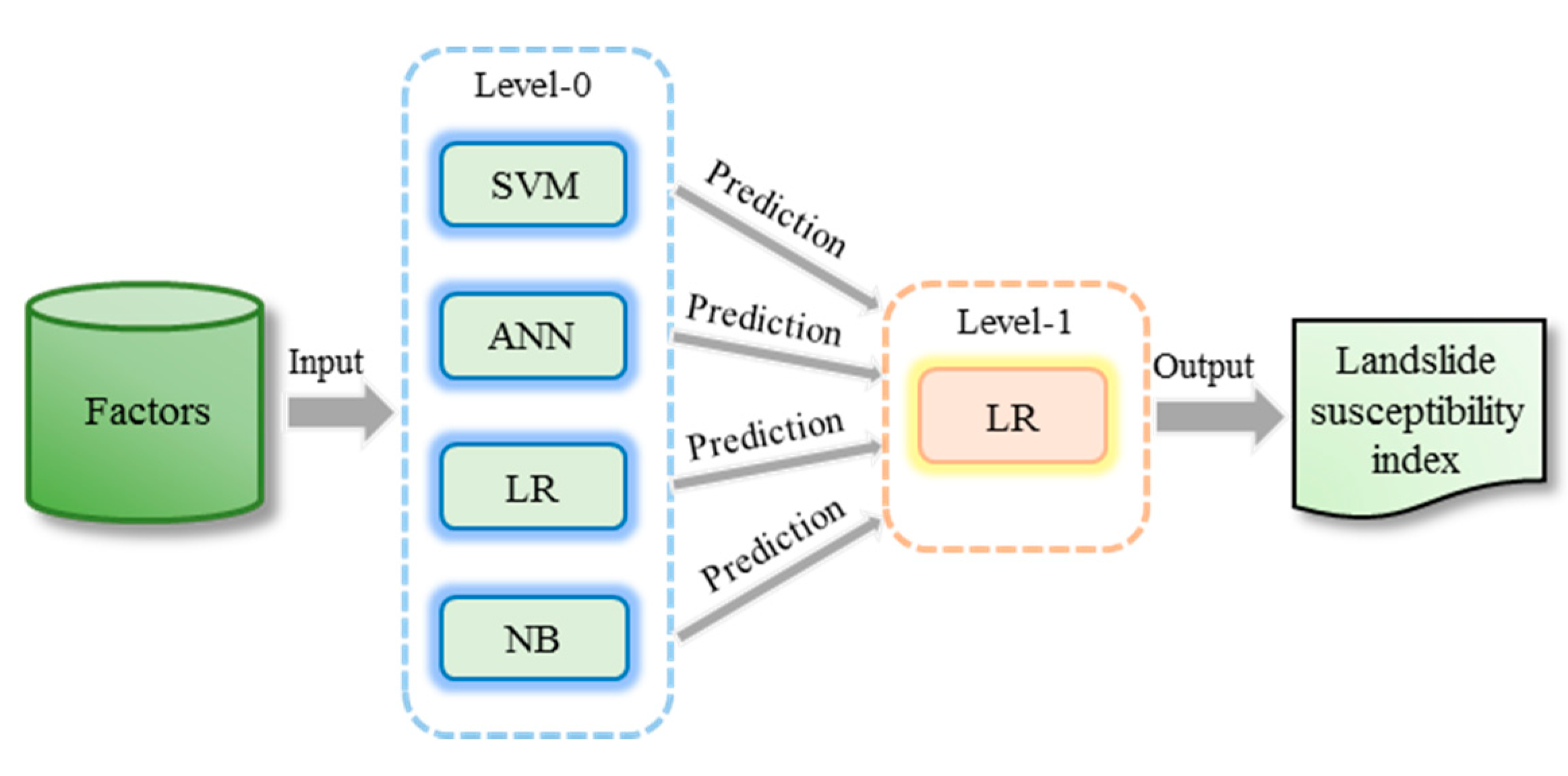
3.4.5. Ensemble Modeling

Once all base learning algorithms are prepared, they are integrated into a whole framework using the stacking method. Suppose the initial dataset$D$ consists of examples $d_i=\left(x_{\mathrm{i}},y_{\mathrm{i}}\right)$, where $x_{\mathrm{i}}$ indicate landslide conditioning factors, and $y_{\mathrm{i}}$ indicates corresponding classifications (landslide or non-landslide). $\mathrm{i}\in \left[1,\mathrm{N}\right]$, where N represents the total number of the modeling dataset. Base learning algorithms such as SVM, ANN, LR, and NB are denoted as $L_t\left(\mathrm{t}=1,2,3,4\right)$. Firstly, the dataset$D$ is repeatedly divided into two disjoint subsets; one is used to train base learning algorithms to generate level-0 classifiers, noted as $h_t$:

$$h_t^i=L_t\left(D-d_i\right)\forall \mathrm{i}=1,2,\cdots ,\mathrm{N};\forall \mathrm{t}=1,2,3,4$$

(7)

The remaining examples are used to make predictions ($z_{it}$) through trained classifiers:

$$z_{it}=h_t^i\left(x_i\right)$$

(8)

These outputs from level-0 classifiers along with their true classification comprise a new dataset $D^{\prime }$ = $\left(\left(z_{it},z_{it},\cdots ,z_{it}\right),y_i\right)$, and are then fed to level-1 to train the meta-learner (LR). Thus, LR can assemble the classification results of base learners to produce the final prediction for new cases:

$$Y_x=LR\left(h_1\left(x\right),h_2\left(x\right),h_3\left(x\right),h_4\left(x\right)\right)$$

(9)

Based on four single candidate algorithms and the stacking technique, the initial ensemble model was constructed, denoted as the SVM–ANN–NB–LR (SANL).

3.5. Resampling Strategy and Correlation Analysis

In statistical learning, an experiment with the purpose of comparing and ranking several algorithms in terms of a certain performance measure is referred to as a benchmark experiment. The resampling strategy is usually utilized to generate point estimations for the performance, which allows for an observation on the performance distribution of an algorithm on resampled subsets [75]. In this work, resampling was used as a pretreatment method for evaluating the correlation between candidate algorithms (Figure 6).

To be specific, when an ensemble model was simulated and constructed in the training stage, the training data could be randomly divided into ten folds to test single base learners. Each fold data was used to produce a prediction by a base learner, and then its prediction accuracy on this fold was recorded. This processing was repeated with n rounds. In other words, n × 10 different subsets with the same size were randomly resampled from the initial training data, and thus n × 10 accuracy values were obtained for each base learner. In this study, we set n as 2, 3, and 4 to produce 20 resamples, 30 resamples, and 40 resamples, respectively. Recalling the processing of resampling, for each resampled subset, four base learners produced prediction in parallel. As resampling proceeded, a series of point estimates of prediction accuracy was derived. Thus, the correlation between base learners could be measured according to the variation degree of those prediction accuracy pairs over the change of subset.

Pearson’s correlation analysis is considered as an effective method to estimate the linear correlative degree between variables [76]. Therefore, the correlation between those base learners was measured using Pearson’s correlation coefficient (PCC) in this study. The PCC between two base learners $L_i$ and $L_j$ is defined as below:

$$PCC\left(L_i,L_j\right)=\frac{cov\left(AC{C}_i,AC{C}_j\right)}{\sqrt{var\left(AC{C}_i\right)\times var\left(AC{C}_j\right)}}$$

(10)

where$cov\left(AC{C}_i,AC{C}_j\right)$ is the covariance, and $AC{C}_i$ and $AC{C}_j$ are respectively the predictive accuracy sets of $L_i$ and $L_i$. $var\left(AC{C}_i\right),$ and $var\left(AC{C}_j\right)$ are respectively the variance of $AC{C}_i$ and $AC{C}_j$.

4. Results

4.1. Selection of Conditioning Factors

The IV evaluation method was carried out to analyze the importance of landslide conditioning factors, and the results are presented in

Table 2. Information value (IV) analysis of landslide conditioning factors.

Conditioning Factors	Classes	Numbers of Landslide Pixel	Numbers of Non- Landslide Pixel	IV of Classes	IV of Factors
Distance to roads (m)	0–67.26	144	27,281	0.408	3.329
	67.26–179.97	115	35,161	0.180
	179.97–430.47	75	51,765	0.003
	430.47–803.09	32	45,260	0.036
	803.09–2048.00	19	70,570	0.261
	2048.00–2556.69	3	16,078	0.108
	>2556.69	0	64,101	2.333
Elevation (m)	740.00–1043.67	88	12,262	0.334	2.694
	1043.67–2138.90	271	105,623	0.254
	2138.90–2389.03	25	35,515	0.025
	2389.03–4160.00	4	156,816	2.081
Land use	Residential area	36	1951	0.233	1.136
	Forest	146	247,017	0.315
	Grassland	20	26,894	0.018
	Farmland	33	3918	0.138
	Bare land	131	28,544	0.319
	Engineering land	2	169	0.010
	Other	20	1723	0.103
NDVI	−1–0.12	10	28,751	0.087	1.089
	0.12–0.35	97	19,308	0.282
	0.35–0.58	144	50,805	0.168
	0.58–0.75	62	38,833	0.006
	0.75–0.89	38	39,805	0.008
	0.89–1	37	132,714	0.539
Distance to faults(m)	0–583.52	226	101,844	0.148	0.733
	583.52–1782.99	125	83,965	0.009
	1782.99–2317.76	18	18,050	0.004
	>2317.76	19	106,357	0.572
ERG	1	131	110,304	0.001	0.396
	2	0	335	0.007
	3	104	63,313	0.017
	4	36	26,766	0.001
	5	52	21,698	0.042
	6	30	81,418	0.226
	7	35	6382	0.103
Slope angle (°)	0–6.22	18	5105	0.035	0.176
	6.22–21.27	126	63,154	0.054
	21.27–32.86	156	121,863	0.000
	>32.86	88	120,094	0.086
Profile curvature	−16.00–0.04	106	130,893	0.068	0.105
	−0.04–26.53	282	179,323	0.037
Slope aspect (°)	0–302.33	358	262,403	0.007	0.065
	>302.33	30	47,813	0.057
Annual rainfall (mm)	773.87–1210.57	292	202,052	0.015	0.052
	1210.57–1419.27	96	108,164	0.037
Distance to rivers (m)	0–272.17	199	124,775	0.027	0.050
	272.17–2566.56	189	185,441	0.023
Plan curvature	−28.56–20.05	388	310,216	0.000	0.000

. It can be observed that the distance to roads gained a highest IV value of 3.329 among all factors, followed by elevation (2.694), land use (1.136), NDVI (1.0894), distance to faults (0.733), ERG (0.396), slope angle (0.176), profile curvature (0.105), slope aspect (0.065), annual rainfall (0.052), distance to rivers (0.050), and plan curvature (0), respectively. This result indicates that distance to roads was the most important factor responsible for landslide susceptibility assessment in the study area. Previous studies emphasized the role of roads, as excavation activities and removal of vegetation during road constructions usually disturb natural terrain and interfere with slope stability [32]. In addition, the effect of faults can never be neglected in landslide analysis. The integrity of rock in the neighboring area of faults is disturbed by fault activities, which makes it prone to weathering and benefits to landslide [77]. Cracks and joints induced by faults also contribute to the enrichment and infiltration process of rainwater and groundwater. It should be noted that the spatial variation of plan curvature fails to distinguish the landslide-prone areas effectively. Therefore, plan curvature was eliminated from landslide modeling owing to its incompetence.

4.2. Appropriateness Evaluation for Base Learners

The appropriateness of a base learner to the ensemble was evaluated mainly through the correlation analysis. However, in order to verify the improved role of the stacking-based ensemble, the performance of its single counterparts integrated into the whole ensemble framework still needed to be presented. In the stage of resampling, a series of predictive accuracies were recorded for each base learner as the subset was constantly sampled. To observe the accuracy distribution, a density curve was created by plotting the accuracy value on the x-axis and the corresponding frequency of the accuracy on the y-axis. Figure 7 shows the density curves for all base learners in terms of 20, 30, and 40 resamples, respectively. In general, it is preferable to use a specific value to describe a model’s performance. Thus, the mean accuracy (MACC) was used to quantify the performance of base learners against the ensemble. Regarding the 20 resamples, the ANN showed the highest MACC with a value of 84.20%, followed by the SVM (83.92%), NB (82.63%), and LR (81.00%), respectively. In the case of 30 resamples, the highest MACC was also achieved by the ANN (84.49%), followed by the SVM (84.01%), NB (82.36%), and LR (81.26%), respectively. As for 40 resamples, the results showed a similar ranking, as the ANN gained the highest MACC value of 84.38%, followed by the SVM (83.92%), NB (82.68%), and LR (81.17%), respectively. Consistently, the results demonstrated the ANN had a slightly better performance than the SVM, NB, and LR.

The scatter-plot matrix of the accuracy belonging to corresponding pairs of base learners is shown in Figure 8. This allowed for a pair-wise comparison to base learners. The correlation between base learners is an estimation of how closely the scatter points of the accuracy lie to the straight line. Visual inspection of Figure 8 shows that the scatter belonging to the pair of SVM and LR was roughly linear. The PCC provided a quantitative measure for this correlation, and its result revealed that the highest correlated pair was the SVM and LR regardless of 20, 30, or 40 resamples, with PCC values of 0.75, 0.73, and 0.68, respectively. The mean of PCC (MPCC) reached to 0.72, which was considered as a value indicating a strong correlation. The remaining pairs were weakly or not highly correlated, with MPCC values of 0.37, 0.33, 0.59, 0.47, and 0.42 for NB/SVM, NB/LR, NB/ANN, SVM/ANN, LR/ANN, and LR/SVM, respectively. On average, pairs that contained the NB had the lowest PCCs.

If highly correlated base learning algorithms are considered to be inappropriate components in ensemble modeling, they should be excluded from the initial ensemble model. According to the PCC results, the LR and SVM were separately eliminated from the SANL model to produce the SVM-ANN-NB (SAN) model and the ANN-NB-LR (ANL) model. Furthermore, in order to verify the weakly correlated base learners are good candidates, the NB was also removed from the SANL model, and the SVM-ANN-LR (SAL) model was further constructed. As a result, a total of four ensemble models were prepared for the experiments and their performances were evaluated and compared.

4.3. Landslide Susceptibility Assessment Using Ensemble Modeling

As the main goal of this study is to examine the “optimal” ensemble on the basis of available candidates for landslide susceptibility assessment, the susceptibility maps of the study area are developed mainly using four ensemble models. Once ensemble modeling was successfully implemented, landslide conditioning factors were fed into the model to produce predictions for the whole area. Thus, each pixel in the study area was allocated a unique landslide susceptibility index (LSI). The higher the index value, the more susceptible the location. Those values were then categorized into five levels, namely, very low, low, moderate, high, and very high by using the geometrical interval classification technique in ArcGIS 10.2 software. Inspection of Figure 9 shows that a similar distribution pattern of landslide susceptibility was gained for various models, especially for the SAN model and the ANL model. All ensemble models were in accordance with the in that areas with very high susceptibility classes were mainly distributed near the Nujiang River Grand Canyon where strong tectonic breaks disturb the terrain, and that the developed road system in conjunction with low vegetation coverage in low-elevation areas further promoted slope instability. Clay-bearing rocks (e.g., mudstones and shales) and sediments play an important role in slope sliding as they contribute to the infiltration process [24]. Additionally, carbonate rocks are likely to be located in highly vulnerable areas because they are prone to weathering which damages slope stability. The visual inspection of the geological map indicates that landslides were related to these negative geologic conditions.

Statistical results on the percentage of landslide pixels (PL) and the percentage of pixels in a susceptibility class (PC) are summarized in

Table 3. Landslide density analysis on landslide susceptibility maps. LD: landslide density; PC: percentage of pixels in a susceptibility class; PL: percentage of landslide pixels.

Class	SANL			SAN			ANL			SAL
	PC (%)	PL (%)	LD	PC (%)	PL (%)	LD	PC (%)	PL (%)	LD	PC (%)	PL (%)	LD
Very low	35.60	0.00	0.00	36.16	0.00	0.00	36.79	0.00	0.00	27.81	0.26	0.01
Low	13.32	0.77	0.06	13.24	0.52	0.04	12.47	0.52	0.04	20.84	0.52	0.02
Moderate	8.13	2.06	0.25	7.89	2.06	0.26	7.88	2.32	0.29	7.20	1.55	0.21
High	26.14	27.32	1.05	19.82	13.66	0.69	21.04	17.78	0.85	32.35	39.95	1.23
Very high	16.80	69.85	4.16	22.90	83.76	3.66	21.82	79.38	3.64	11.80	57.73	4.89

. Regarding the SANL model, 69.85% of the total landslides were located in the very high class that accounted for 16.80% of the total study area, whereas 83.76% of the total landslides occurred in the very highly susceptible areas (22.90%) using the SAN model. As for ANL and SAL models, 79.38% and 57.73% of the total landslides fell into very highly vulnerable classes, while very high classes occupied 21.82% and 11.80% of the total study area, respectively.

Furthermore, the reliability of landslide susceptibility mapping was evaluated using landslide density (LD) analysis. LD is expressed by a ratio of PL and PC [2]. It can be observed from Table 3 that LD values consistently increased from very low susceptibility level to very high susceptibility level for all ensemble models, indicating the developed landslide susceptibility assessment was reasonable.

4.4. Performance Evaluation of Landslide Models

The model evaluation was performed using both the training set and validation set. The former shows the model’s fitting skill and the latter reflects its generalization ability. The accuracy (ACC), Kappa coefficient (K), and the receiver operating characteristic (ROC) curve technique were employed as performance metrics in this study. The ACC is the ratio of landslide and non-landslide grid cells that are correctly predicted, while the K measures the reliability of a constructed model. As for the ROC curve, it is a popular method to evaluate the performance of the landslide model [78,79]. The area under the ROC curve (AUC) value is the area under the ROC curve, and a higher AUC value indicates the model is better.

The overall performance is shown in

Table 4. Performance evaluation of landslide models. AUC: the area under the receiver operating characteristic (ROC) curve; K: Kappa coefficient.

Models	On the Training Stage			On the Validation Stage
	ACC (%)	K	AUC	ACC (%)	K	AUC
SANL	86.40	0.728	0.945	85.34	0.707	0.931
SAN	86.95	0.739	0.951	85.34	0.707	0.940
ANL	86.58	0.732	0.944	85.34	0.707	0.932
SAL	84.93	0.699	0.927	82.33	0.647	0.886

and Figure 10. All ensemble models performed well in goodness of fit as well as generalization ability. Note that the SANL model, the SAN model, and the ANL model yielded almost equal values with respect to the ACC, K, and AUC, but in detail the SAN model (with the ACC, K, and AUC values of 86.95%, 0.739, and 0.951) and the ANL model (with the ACC, K, and AUC values of 86.58%, 0.732, and 0.944) gained slightly better goodness of fit than the SANL model (with ACC, K, and AUC values of 86.40%, 0.728, and 0.945, respectively). The SAL model had a relatively lower performance especially in generalization ability, with values of 82.33%, 0.647, and 0.886 for ACC, K, and AUC, respectively, on the validation set.

5. Discussion

Landslide susceptibility mapping aims to detect the vulnerable areas potentially threatened by landslide geo-hazards. Over the years, advancements in computer technology, the development of machine learning methods, the availability of multi-source data such as GIS data and remote sensing data, and the accessibility of convenient software have facilitated the conduction of landslide susceptibility assessment. In this context, how to improve the accuracy of assessment results has become the main concern of researchers [5]. Recently, ensemble techniques have proved to be able to provide a more accurate solution in landslide susceptibility modeling. In this work, we attempted to use a meta-learning method, namely the stacking ensemble method, to integrate multiple different algorithms. When the predictive accuracy was used as the measure, the ensemble of the SVM-ANN-NB-LR was found to be superior to all single algorithms. The advantage of stacking is reflected in that the two-level framework can learn more classification information, and meta-learner in the high level is capable of correcting bias generated in the former level [80,81]. In this study, the stacking ensemble model showed improved performance against their components, and can be considered as a promising method for landslide susceptibility mapping.

In general, combining several algorithms enables an ensemble model to gain better performance [29]. However, is it necessary to use all of them to constitute the ensemble when multiple predictors are available? For landslide susceptibility modeling, this needs to be investigated. In the field of machine learning, Zhou [82] introduced the concept of the selective ensemble, that is, making appropriate choices from multiple solutions and then combining those selected solutions to obtain the final decision. Similarly, Zeng et al. [83] proposed the selecting base classifiers on bagging (SBCB) algorithm, which proved to be superior to the original bagging method. Determining suitable base learning algorithms is important to examine the “optimal” landslide susceptibility assessment when ensemble modeling is the case. Rossi et al. [44] found the combination of LDA-QDA-LR had a better generalization capability than the combination of LDA-QDA-LR-ANN because the ANN overfitted the landslide information in the training stage. Chen et al. [24] investigated the SVM, ANN, and ME accompanied by their possible ensembles of ANN-SVM, ANN-ME, SVM-ME, and ANN-ME-SVM for landslide susceptibility mapping. They concluded that synergic interaction of two best single models, namely the SVM and ANN, constituted a stronger bond compared with remaining modeling methods. The ensemble models containing the ME showed moderate performance due to the underperformance of the ME model. This result is quite consistent with a gully erosion modeling study which reported that single models with good performance such as SVM and ANN played an improver role in ensemble modeling, while the relatively weak model (e.g., ME) acted as a depriver [84]. A powerful model tends to add positive properties to subordinate models. To put it in another way, the outperformance of the ensemble depends mainly on good components. Therefore, the best base learner, e.g., the ANN used in this study, should be included in ensemble modeling to maintain the outperformance. In contrast, the base learner with a relatively poor performance that may play a reducer role seems to be inappropriate for constituting the ensemble. However, all base learners used in this study achieved good predictive accuracies. Here, “slightly weak” is a relative concept; the threshold for positive synergy among base learners may be difficult to determine [24]. In addition, it is also questionable to explain the extremely similar behaviors between the SAN model and the ANL model only judged by the component’s performance, because removing SVM or LR from the initial ensemble of the SVM-ANN-NB-LR has an equal effect in the case where the SVM outperformed the LR.

To address this issue, we introduced a resampling scheme and correlation analysis for estimating the correlation between base learners within the ensemble. When constituting the ensemble, it is desirable that the predictions produced by base learners be weakly correlated as the similar predictions may not contribute to the ensemble performance. In this study, the PCC values under different resampling times (with the 20, 30, and 40 times, respectively) showed a high correlation between the SVM and LR. This result means the SVM generates very similar or even the same predictions as the LR for ensemble modeling in most cases, reducing the effect of assembling predictions. In other words, the SVM and LR played an equal role in the ensemble of SVM-ANN-NB-LR, which led to similar performances between the SAN model and the ANL model, as well as similar distribution patterns of developed susceptibility maps. In fact, the SANL model also behaved similarly to the SAN model and the ANL model. We argue that the performance evaluation for the candidate used for composing the ensemble is important but may not be conclusive, because all base learners yielded good predictive accuracies in this work. In this case, a correlation analysis is helpful to determine eligible candidates for “optimal” landslide ensemble modeling. We further verified this by removing the NB from the SANL model, and it was found that the SAL model underperformed the other ensemble models. The correlation analysis showed pairs containing the NB had the lowest PCC on average results. The decreased performance of ensemble modeling after excluding the NB indicated that weakly or not highly correlated candidates should be included in the ensemble. Overall, our results suggest that the candidates serving as base learners should be skillful but diverse, allowing the ensemble method to determine how to combine the best solutions from base learners for performance refinement [85,86].

However, some limitations should be noted. When it comes to such geologic factors as modeling input, we considered the physical and mechanical properties of engineering rock groups alone without taking into account geologic factors such as the angle of rock bedding and the orientation of bedding relative to slope direction that are related to slope failure. As detailed knowledge of geology is critical for landslide susceptibility studies, we will focus more on these important geologic factors and examine their effect in the future work.

6. Conclusions

Landslide modeling in this study mainly served two goals: (1) to investigate the stacking ensemble technique for landslide susceptibility assessment; and (2) to set a strategy to determine appropriate combinations when multiple candidates were available in ensemble learning. Before modeling, the IV evaluation was carried out for feature selection. It was found that of the initially prepared factors, eleven of them, namely distance to roads, elevation, land use, NDVI, distance to faults, ERG, slope angle, profile curvature, slope aspect, annual rainfall, and distance to rivers, were finally identified as inputs for ensemble modeling. The performance evaluation showed that the stacking ensemble-based susceptibility mapping procedure could make full use of the advantages of various individual models and achieve an improved prediction accuracy, indicating that stacking was also a promising method for landslide susceptibility mapping. Moreover, the resampling strategy and Pearson’s correlation analysis were jointly used to test the correlation between base learners. The SVM and LR were highly correlated within the ensemble of the SANL, which resulted in the similar behaviors of the SANL model, the SAN model, and the ANL model. This result implies highly correlated candidates may be inappropriate for being combined in an ensemble prediction. As a result, the use of the SAN model or the ANL model instead of the SANL model is feasible for landslide susceptibility mapping in the study area. The findings and analysis from this study present the advantages of the stacking ensemble method, and provide an accessible way to select good candidates for ensemble modeling, which may be helpful for future landslide susceptibility studies.

References

1. Gutiérrez, F.; Linares, R.; Roqué, C.; Zarroca, M.; Carbonel, D.; Rosell, J.; Gutiérrez, M. Large landslides associated with a diapiric fold in Canelles Reservoir (Spanish Pyrenees): Detailed geological–geomorphological mapping, trenching and electrical resistivity imaging. Geomorphology 2015, 241, 224–242. [Google Scholar] [CrossRef]
2. Pham, B.T.; Pradhan, B.; Tien Bui, D.; Prakash, I.; Dholakia, M.B. A comparative study of different machine learning methods for landslide susceptibility assessment: A case study of Uttarakhand area (India). Environ. Model. Softw. 2016, 84, 240–250. [Google Scholar] [CrossRef]
3. Song, Y.; Gong, J.; Gao, S.; Wang, D.; Cui, T.; Li, Y.; Wei, B. Susceptibility assessment of earthquake-induced landslides using Bayesian network: A case study in Beichuan, China. Comput. Geosci. 2012, 42, 189–199. [Google Scholar] [CrossRef]
4. Jiao, Y.; Zhao, D.; Ding, Y.; Liu, Y.; Xu, Q.; Qiu, Y.; Liu, C.; Liu, Z.; Zha, Z.; Li, R. Performance evaluation for four GIS-based models purposed to predict and map landslide susceptibility: A case study at a World Heritage site in Southwest China. Catena 2019, 183, 104–221. [Google Scholar] [CrossRef]
5. Dou, J.; Yunus, A.P.; Bui, D.T.; Merghadi, A.; Sahana, M.; Zhu, Z.; Chen, C.W.; Han, Z.; Pham, B.T. Improved landslide assessment using support vector machine with bagging, boosting, and stacking ensemble machine learning framework in a mountainous watershed, Japan. Landslides 2019. [Google Scholar] [CrossRef]
6. Dahal, R.K.; Hasegawa, S.; Nonomura, A.; Yamanaka, M.; Dhakal, S.; Paudyal, P. Predictive modelling of rainfall-induced landslide hazard in the Lesser Himalaya of Nepal based on weights-of-evidence. Geomorphology 2008, 102, 496–510. [Google Scholar] [CrossRef]
7. Guzzetti, F.; Carrara, A.; Cardinali, M.; Reichenbach, P. Landslide hazard evaluation: A review of current techniques and their application in a multi-scale study, Central Italy. Geomorphology 1999, 31, 181–216. [Google Scholar] [CrossRef]
8. Korup, O.; Stolle, A. Landslide prediction from machine learning. Geol. Today 2014, 30, 26–33. [Google Scholar] [CrossRef]
9. Suzen, M.L.; Kaya, B.Ş. Evaluation of environmental parameters in logistic regression models for landslide susceptibility mapping. Int. J. Digit. Earth 2012, 5, 338–355. [Google Scholar] [CrossRef]
10. Wang, L.J.; Sawada, K.; Moriguchi, S. Landslide susceptibility analysis with logistic regression model based on FCM sampling strategy. Comput. Geosci. 2013, 57, 81–92. [Google Scholar] [CrossRef]
11. Dimri, S.; Lakhera, R.C.; Sati, S. Fuzzy-based method for landslide hazard assessment in active seismic zone of Himalaya. Landslides 2007, 4, 101–110. [Google Scholar] [CrossRef]
12. Feizizadeh, B.; Blaschke, T.; Roodposhti, M.S. Integrating GIS Based Fuzzy Set Theory in Multicriteria Evaluation Methods for Landslide Susceptibility Mapping. Int. J. Geoinformatics 2013, 9, 49–57. [Google Scholar]
13. Park, N.W. Using maximum entropy modeling for landslide susceptibility mapping with multiple geoenvironmental data sets. Environ. Earth Sci. 2015, 73, 937–949. [Google Scholar] [CrossRef]
14. Zare, M.; Pourghasemi, H.R.; Vafakhah, M.; Pradhan, B. Landslide susceptibility mapping at Vaz Watershed (Iran) using an artificial neural network model: A comparison between multilayer perceptron (MLP) and radial basic function (RBF) algorithms. Arab. J. Geosci. 2013, 6, 2873–2888. [Google Scholar] [CrossRef]
15. Conforti, M.; Pascale, S.; Robustelli, G.; Sdao, F. Evaluation of prediction capability of the artificial neural networks for mapping landslide susceptibility in the Turbolo River catchment (northern Calabria, Italy). Catena 2014, 113, 236–250. [Google Scholar] [CrossRef]
16. Oh, H.-J.; Lee, S. Shallow Landslide Susceptibility Modeling Using the Data Mining Models Artificial Neural Network and Boosted Tree. Appl. Sci. 2017, 7, 1000. [Google Scholar] [CrossRef] [Green Version]
17. Tien Bui, D.; Pradhan, B.; Lofman, O.; Revhaug, I. Landslide Susceptibility Assessment in Vietnam Using Support Vector Machines, Decision Tree, and Naïve Bayes Models. Math. Probl. Eng. 2012, 2012, 1–26. [Google Scholar] [CrossRef] [Green Version]
18. Xu, C.; Dai, F.; Xu, X.; Lee, Y.H. GIS-based support vector machine modeling of earthquake-triggered landslide susceptibility in the Jianjiang River watershed, China. Geomorphology 2012, 145, 70–80. [Google Scholar] [CrossRef]
19. Hong, H.; Pradhan, B.; Xu, C.; Bui, D.T. Spatial prediction of landslide hazard at the Yihuang area (China) using two-class kernel logistic regression, alternating decision tree and support vector machines. Catena 2015, 133, 266–281. [Google Scholar] [CrossRef]
20. Yao, X.; Than, L.G.; Dai, F.C. Landslide susceptibility mapping based on Support Vector Machine: A case study on natural slopes of Hong Kong, China. Geomorphology 2008, 101, 572–582. [Google Scholar] [CrossRef]
21. Youssef, A.M.; Pourghasemi, H.R.; Pourtaghi, Z.S.; Al-Katheeri, M.M. Landslide susceptibility mapping using random forest, boosted regression tree, classification and regression tree, and general linear models and comparison of their performance at Wadi Tayyah Basin, Asir Region, Saudi Arabia. Landslides 2016, 13, 839–856. [Google Scholar] [CrossRef]
22. Felicísimo, Á.M.; Cuartero, A.; Remondo, J.; Quirós, E. Mapping landslide susceptibility with logistic regression, multiple adaptive regression splines, classification and regression trees, and maximum entropy methods: A comparative study. Landslides 2013, 10, 175–189. [Google Scholar] [CrossRef]
23. Chen, W.; Xie, X.; Wang, J.; Pradhan, B.; Hong, H.; Bui, D.T.; Duan, Z.; Ma, J. A comparative study of logistic model tree, random forest, and classification and regression tree models for spatial prediction of landslide susceptibility. Catena 2017, 151, 147–160. [Google Scholar] [CrossRef] [Green Version]
24. Chen, W.; Pourghasemi, H.R.; Kornejady, A.; Zhang, N. Landslide spatial modeling: Introducing new ensembles of ANN, MaxEnt, and SVM machine learning techniques. Geoderma 2017, 305, 314–327. [Google Scholar] [CrossRef]
25. Tien Bui, D.; Shirzadi, A.; Shahabi, H.; Geertsema, M.; Omidvar, E.; Clague, J.; Thai Pham, B.; Dou, J.; Talebpour Asl, D.; Bin Ahmad, B.; et al. New Ensemble Models for Shallow Landslide Susceptibility Modeling in a Semi-Arid Watershed. Forests 2019, 10, 743. [Google Scholar] [CrossRef] [Green Version]
26. Merghadi, A.; Abderrahmane, B.; Tien Bui, D. Landslide Susceptibility Assessment at Mila Basin (Algeria): A Comparative Assessment of Prediction Capability of Advanced Machine Learning Methods. ISPRS Int. J. Geo-Inf. 2018, 7, 268. [Google Scholar] [CrossRef] [Green Version]
27. Lee, J.H.; Sameen, M.I.; Pradhan, B.; Park, H.J. Modeling landslide susceptibility in data-scarce environments using optimized data mining and statistical methods. Geomorphology 2018, 303, 284–298. [Google Scholar] [CrossRef]
28. Hong, H.; Liu, J.; Bui, D.T.; Pradhan, B.; Acharya, T.D.; Pham, B.T.; Zhu, A.X.; Chen, W.; Ahmad, B.B. Landslide susceptibility mapping using J48 Decision Tree with AdaBoost, Bagging and Rotation Forest ensembles in the Guangchang area (China). Catena 2018, 163, 399–413. [Google Scholar] [CrossRef]
29. Rokach, L. Taxonomy for characterizing ensemble methods in classification tasks: A review and annotated bibliography. Comput. Stat. Data Anal. 2009, 53, 4046–4072. [Google Scholar] [CrossRef] [Green Version]
30. Zhou, Z. Ensemble learning. Encycl. Biom. 2009, 1, 411–416. [Google Scholar]
31. Tien Bui, D.; Ho, T.-C.; Pradhan, B.; Pham, B.-T.; Nhu, V.-H.; Revhaug, I. GIS-based modeling of rainfall-induced landslides using data mining-based functional trees classifier with AdaBoost, Bagging, and MultiBoost ensemble frameworks. Environ. Earth Sci. 2016, 75. [Google Scholar] [CrossRef]
32. Pham, B.T.; Tien Bui, D.; Prakash, I.; Dholakia, M.B. Hybrid integration of Multilayer Perceptron Neural Networks and machine learning ensembles for landslide susceptibility assessment at Himalayan area (India) using GIS. Catena 2017, 149, 52–63. [Google Scholar] [CrossRef]
33. Truong, X.; Mitamura, M.; Kono, Y.; Raghavan, V.; Yonezawa, G.; Truong, X.; Do, T.; Tien Bui, D.; Lee, S. Enhancing Prediction Performance of Landslide Susceptibility Model Using Hybrid Machine Learning Approach of Bagging Ensemble and Logistic Model Tree. Appl. Sci. 2018, 8, 1046. [Google Scholar] [CrossRef] [Green Version]
34. Chen, W.; Shahabi, H.; Zhang, S.; Khosravi, K.; Shirzadi, A.; Chapi, K.; Pham, B.; Zhang, T.; Zhang, L.; Chai, H.; et al. Landslide Susceptibility Modeling Based on GIS and Novel Bagging-Based Kernel Logistic Regression. Appl. Sci. 2018, 8, 2540. [Google Scholar] [CrossRef] [Green Version]
35. Park, S.; Kim, J. Landslide Susceptibility Mapping Based on Random Forest and Boosted Regression Tree Models, and a Comparison of Their Performance. Appl. Sci. 2019, 9, 942. [Google Scholar] [CrossRef] [Green Version]
36. Pham, B.T.; Prakash, I.; Singh, S.K.; Shirzadi, A.; Shahabi, H.; Tran, T.-T.-T.; Bui, D.T. Landslide susceptibility modeling using Reduced Error Pruning Trees and different ensemble techniques: Hybrid machine learning approaches. Catena 2019, 175, 203–218. [Google Scholar] [CrossRef]
37. Breiman, L. Bagging predictors. Mach. Learn. 1996, 24, 123–140. [Google Scholar] [CrossRef] [Green Version]
38. Schapire, R.E. The strength of weak learnability. Mach. Learn. 1990, 5, 197–227. [Google Scholar] [CrossRef] [Green Version]
39. Freund, Y.; Schapire, R.E. A decision-theoretic generalization of on-line learning and an application to boosting. J. Comput. Syst. Sci. 1997, 55, 119–139. [Google Scholar] [CrossRef] [Green Version]
40. Breiman, L. Random forest. Mach. Learn. 2001, 45, 5–32. [Google Scholar] [CrossRef] [Green Version]
41. Rodriguez, J.J.; Kuncheva, L.I.; Alonso, C.J. Rotation forest: A new classifier ensemble method. IEEE Trans. Pattern Anal. Mach. Intell. 2006, 28, 1619–1630. [Google Scholar] [CrossRef] [PubMed]
42. Lee, S.; Ryu, J.H.; Won, J.S.; Park, H.J. Determination and application of the weights for landslide susceptibility mapping using an artificial neural network. Eng. Geol. 2004, 71, 289–302. [Google Scholar] [CrossRef]
43. Kanungo, D.P.; Arora, M.K.; Sarkar, S.; Gupta, R.P. A comparative study of conventional, ANN black box, fuzzy and combined neural and fuzzy weighting procedures for landslide susceptibility zonation in Darjeeling Himalayas. Eng. Geol. 2006, 85, 347–366. [Google Scholar] [CrossRef]
44. Rossi, M.; Guzzetti, F.; Reichenbach, P.; Mondini, A.C.; Peruccacci, S. Optimal landslide susceptibility zonation based on multiple forecasts. Geomorphology 2010, 114, 129–142. [Google Scholar] [CrossRef]
45. Aghdam, I.N.; Varzandeh, M.H.M.; Pradhan, B. Landslide susceptibility mapping using an ensemble statistical index (Wi) and adaptive neuro-fuzzy inference system (ANFIS) model at Alborz Mountains (Iran). Environ. Earth Sci. 2016, 75, 1–20. [Google Scholar] [CrossRef]
46. Wang, G.; Hao, J.; Ma, J.; Jiang, H. A comparative assessment of ensemble learning for credit scoring. Expert Syst. Appl. 2011, 38, 223–230. [Google Scholar] [CrossRef]
47. Shu, C.; Burn, D.H. Artificial neural network ensembles and their application in pooled flood frequency analysis. Water Resour. Res. 2004, 40. [Google Scholar] [CrossRef] [Green Version]
48. Rahali, H. Improving the reliability of landslide susceptibility mapping through spatial uncertainty analysis: A case study of Al Hoceima, Northern Morocco. Geocarto Int. 2017, 34, 43–77. [Google Scholar] [CrossRef]
49. Nsengiyumva, J.B.; Luo, G.; Amanambu, A.C.; Mind’je, R.; Habiyaremye, G.; Karamage, F.; Ochege, F.U.; Mupenzi, C. Comparing probabilistic and statistical methods in landslide susceptibility modeling in Rwanda/Centre-Eastern Africa. Sci. Total Environ. 2019, 659, 1457–1472. [Google Scholar] [CrossRef] [PubMed] [Green Version]
50. Pourghasemi, H.R.; Kerle, N. Random forests and evidential belief function-based landslide susceptibility assessment in Western Mazandaran Province, Iran. Environ. Earth Sci. 2016, 75, 185. [Google Scholar] [CrossRef]
51. Juliev, M.; Mergili, M.; Mondal, I.; Nurtaev, B.; Pulatov, A.; Hubl, J. Comparative analysis of statistical methods for landslide susceptibility mapping in the Bostanlik District, Uzbekistan. Sci. Total Environ. 2019, 653, 801–814. [Google Scholar] [CrossRef] [PubMed]
52. Grelle, G.; Soriano, M.; Revellino, P.; Guerriero, L.; Anderson, M.G.; Diambra, A.; Fiorillo, F.; Esposito, L.; Diodato, N.; Guadagno, F.M. Space–time prediction of rainfall-induced shallow landslides through a combined probabilistic/deterministic approach, optimized for initial water table conditions. Bull. Eng. Geol. Environ. 2013, 73, 877–890. [Google Scholar] [CrossRef]
53. Bennett, G.L.; Miller, S.R.; Roering, J.J.; Schmidt, D.A. Landslides, threshold slopes, and the survival of relict terrain in the wake of the Mendocino Triple Junction. Geology 2016, 44, 363–366. [Google Scholar] [CrossRef] [Green Version]
54. Kornejady, A.; Ownegh, M.; Bahremand, A. Landslide susceptibility assessment using maximum entropy model with two different data sampling methods. Catena 2017, 152, 144–162. [Google Scholar] [CrossRef]
55. MacQueen, J. Some Methods for classification and Analysis of Multivariate Observations. In Proceedings of the Fifth Berkeley Symposium on Mathematical Statistics and Probability, Berkeley, CA, USA, 19 June 1967; Volume 1, pp. 281–297. [Google Scholar]
56. Ghailan, O.; Mokhtar, H.M.; Hegazy, O. Improving Credit Scorecard Modeling Through Applying Text Analysis. Int. J. Adv. Comput. Sci. Appl. 2016, 7, 512–517. [Google Scholar] [CrossRef] [Green Version]
57. Refaat, M. Credit Risk Scorecard: Development and Implementation Using SAS; Lulu: San Francisco, CA, USA, 2011. [Google Scholar]
58. Jopia, H.R. Package ‘Smbinning’ Optimal Binning for Scoring Modeling. Available online: https://www.blog.revolutionanalytics.com201503r-package-smbinning-optimal-binning-for-scoring-modeling.html (accessed on 1 April 2019).
59. Hothorn, T.; Hornik, K.; Zeileis, A. Ctree: Conditional inference trees. Compr. R Arch. Netw. 2015, 1–34. [Google Scholar]
60. Wolpert, D.H. Stacked Generalization. Neural Netw. 1992, 5, 241–259. [Google Scholar] [CrossRef]
61. Zhou, Z. Ensemble Methods: Foundations and Algorithms; Chapman and Hall/CRC: Cambridge, UK, 2012; pp. 1–219. [Google Scholar] [CrossRef]
62. Lee, S.; Ryu, J.H.; Kim, I.S. Landslide susceptibility analysis and its verification using likelihood ratio, logistic regression, and artificial neural network models: Case study of Youngin, Korea. Landslides 2007, 4, 327–338. [Google Scholar] [CrossRef]
63. Tsangaratos, P.; Ilia, I. Comparison of a logistic regression and Naïve Bayes classifier in landslide susceptibility assessments: The influence of models complexity and training dataset size. Catena 2016, 145, 164–179. [Google Scholar] [CrossRef]
64. Ting, K.M.; Witten, L.H. Issues in Stacked Generalization. J. Artif. Intell. Res. 1999, 10, 271–289. [Google Scholar] [CrossRef] [Green Version]
65. Witten, I.H.; Frank, E. Data Mining: Practical Machine Learning Tools and Techniques; Todd Green: Cambridge, MA, USA, 2005; pp. 1–622. [Google Scholar] [CrossRef]
66. Vapnik, V.N. The Nature of Statistical Learning Theory; Springer: New York, NY, USA, 1995. [Google Scholar] [CrossRef]
67. Dixon, B.; Candade, N. Multispectral landuse classification using neural networks and support vector machines: One or the other, or both? Int. J. Remote Sens. 2008, 29, 1185–1206. [Google Scholar] [CrossRef]
68. Tehrany, M.S.; Pradhan, B.; Jebur, M.N. Flood susceptibility mapping using a novel ensemble weights-of-evidence and support vector machine models in GIS. J. Hydrol. 2014, 512, 332–343. [Google Scholar] [CrossRef]
69. Kawabata, D.; Bandibas, J. Landslide susceptibility mapping using geological data, a DEM from ASTER images and an Artificial Neural Network (ANN). Geomorphology 2009, 113, 97–109. [Google Scholar] [CrossRef]
70. Rumelhart, D.E.; Hinton, G.E.; Williams, R.J. Learning representations by back-propagating errors. Cogn. Model. 1988, 5, 1. [Google Scholar] [CrossRef]
71. Pradhan, B.; Lee, S. Delineation of landslide hazard areas on Penang Island, Malaysia, by using frequency ratio, logistic regression, and artificial neural network models. Environ. Earth Sci. 2010, 60, 1037–1054. [Google Scholar] [CrossRef]
72. Kavzoglu, T.; Sahin, E.K.; Colkesen, I. Landslide susceptibility mapping using GIS-based multi-criteria decision analysis, support vector machines, and logistic regression. Landslides 2014, 11, 425–439. [Google Scholar] [CrossRef]
73. Soria, D.; Garibaldi, J.M.; Ambrogi, F.; Biganzoli, E.M.; Ellis, I.O. A ‘Non-Parametric’ Version of the Naive Bayes Classifier. Knowl.-Based Syst. 2011, 24, 775–784. [Google Scholar] [CrossRef] [Green Version]
74. Domingos, P.; Pazzani, M. Beyond independence: Conditions for the optimality of the simple Bayesian classifier. In Proceedings of the 13th Intl. Conf. Machine Learning, Miami, FL, USA, 4–7 December 2013; pp. 105–112. [Google Scholar]
75. Hothorn, T.; Leisch, F.; Zeileis, A.; Hornik, K. The design and analysis of benchmark experiments. J. Comput. Graph. Stat. 2005, 14, 675–699. [Google Scholar] [CrossRef] [Green Version]
76. Rodriguez-Lujan, I.; Huerta, R.; Elkan, C.; Cruz, C.S. Quadratic programming feature selection. J. Mach. Learn. Res. 2010, 11, 1491–1516. [Google Scholar] [CrossRef] [Green Version]
77. Chen, W.; Sun, Z.; Han, J. Landslide Susceptibility Modeling Using Integrated Ensemble Weights of Evidence with Logistic Regression and Random Forest Models. Appl. Sci. 2019, 9, 171–197. [Google Scholar] [CrossRef] [Green Version]
78. Feizizadeh, B.; Roodposhti, M.S.; Jankowski, P.; Blaschke, T. A GIS-based extended fuzzy multi-criteria evaluation for landslide susceptibility mapping. Comput. Geosci. 2014, 73, 208–221. [Google Scholar] [CrossRef] [PubMed] [Green Version]
79. Razavi Termeh, S.V.; Kornejady, A.; Pourghasemi, H.R.; Keesstra, S. Flood susceptibility mapping using novel ensembles of adaptive neuro fuzzy inference system and metaheuristic algorithms. Sci. Total Environ. 2018, 615, 438–451. [Google Scholar] [CrossRef] [PubMed]
80. Menahem, E.; Rokach, L.; Elovici, Y. Troika—An improved stacking schema for classification tasks. Inf. Sci. 2009, 179, 4097–4122. [Google Scholar] [CrossRef] [Green Version]
81. Džeroski, S.; Ženko, B. Is combining classifiers with stacking better than selecting the best one? Mach. Learn. 2004, 54, 255–273. [Google Scholar] [CrossRef] [Green Version]
82. Zhou, Z.; Wu, J.; Wei, T. Ensembling neural networks: Many could be better than all. J. Artif. Intell. 2002, 137, 239–263. [Google Scholar] [CrossRef] [Green Version]
83. Zeng, X.D.; Chao, S.; Wong, F. Optimization of bagging classifiers based on SBCB algorithm. In Proceedings of the 2010 International Conference on Machine Learning and Cybernetics, Qingdao, China, 11–14 July 2010; pp. 262–267. [Google Scholar]
84. Pourghasemi, H.R.; Yousefi, S.; Kornejady, A.; Cerda, A. Performance assessment of individual and ensemble data-mining techniques for gully erosion modeling. Sci. Total Environ. 2017, 609, 764–775. [Google Scholar] [CrossRef] [PubMed] [Green Version]
85. Krogh, A.; Vedelsby, J. Neural network ensembles, cross validation, and active learning. In Proceedings of the 7th International Conference on Neural Information Processing Systems; MIT Press: Cambridge, MA, USA, January 1994; pp. 231–238. [Google Scholar]
86. Kuncheva, L.I.; Whitaker, C.J. Measures of diversity in classifier ensembles. Mach. Learn. 2003, 51, 181–207. [Google Scholar] [CrossRef]
Figure 1. Geographical position of the study area and landslide inventory map.
Applsci 10 04016 g001
Figure 2. Geological map of the study area.
Applsci 10 04016 g002
Figure 3. Landslide conditioning factors (a) Elevation, (b) Slope angle, (c) Slope aspect, (d) Plan curvature, (e) Profile curvature, (f) ERG, (g) Land use, (h) Distance to roads, (i) Distance to rivers, (j) Distance to faults, (k) Annual rainfall, (l) Normalized difference vegetation index (NDVI).
Applsci 10 04016 g003aApplsci 10 04016 g003b
Figure 4. (a) Locations of the selected non-landslide; (b) Distributions of the training dataset and validation dataset. DEM: digital elevation model.
Applsci 10 04016 g004
Figure 5. Stacking-based ensemble framework for landslide susceptibility modeling. SVM: support vector machine; ANN: artificial neural network; LR: logical regression; NB: naive Bayes.
Applsci 10 04016 g005
Figure 6. The flowchart of the resampling strategy and correlation evaluation. ACC: accuracy.
Applsci 10 04016 g006
Figure 7. Density curves of base learners (a) on 20 resamples, (b) on 30 resamples, (c) on 40 resamples. MACC: mean accuracy.
Applsci 10 04016 g007
Figure 8. Scatter-plot matrixes of base learners (a) on 20 resamples, (b) on 30 resamples, (c) on 40 resamples. PCC: Pearson’s correlation coefficient.
Applsci 10 04016 g008
Figure 9. Landslide susceptibility mapping using (a) SVM–ANN–NB–LR (SANL), (b) SVM–ANN–NB (SAN), (c) ANN–NB–LR (ANL), (d) SVM–ANN–LR (SAL).
Applsci 10 04016 g009
Figure 10. ROC analysis of four ensemble models (a) on the training dataset, (b) on the validation dataset. SE: standard error of the AUC; CI: confidence interval of the AUC; p: significance level.
Applsci 10 04016 g010