An Artificial Neural Network Approach to Predicting Most Applicable Post-Contract Cost Controlling Techniques in Construction Projects

Abstract

The post-contract phase of the construction process remains critical to cost management. Several techniques have been used to facilitate effective cost management in this phase. However, the deployment of these techniques has not caused a reduction in the incidence of cost overruns hence casting doubts on their utility. The seeming underwhelming performance posted by these post-contract cost control techniques (PCCTs), has been traced to improper deployment by construction project managers (CPM) and quantity surveyors (QS). Utilizing the perspectives of CPM and QS professionals, as elicited through a survey, produced 135 samples. The instrumentality of the artificial neural networks (ANN) in this study enabled the development of a structured decision-support methodology for analysing the most appropriate PCCTs to be deployed to different construction process phases. Besides showcasing the utility of the emergent ANN-based decision support methodology, the study’s theoretical findings indicate that CPM and QS professionals influence decisions pertaining to PCCTs choice in distinct phases of the construction process. Whereas QS professionals were particularly responsible for the choice of PCCTs during the initial and mid-level phases, CPM professionals assumed responsibility for PCCTs selection during the construction process close-out phase. In construction cost management practice, the crucial PCCTs identifies more with the application of historical data and all cost monitoring approaches.

1. Introduction

Time, cost, and quality remain basic parameters for measuring project management success and by extension, project success [1,2,3]. Therefore, for projects to be adjudged successful, the project management team (PMT) must ensure timely delivery of projects within the projected budget and to the specified quality. Over the years, the increasing inability of PMTs to successfully deliver on these facets enjoys wide reportage in various media. Amongst the three parameters, available evidence indicates a fixation of construction clients on the cost parameter. Often, construction clients have sought greater certainty as it pertains to cost for various reasons. The decision to embark upon a construction project is usually an outcome of the quest to improve service delivery (for public sector clients) or to either improve profitability or reputational capital (private sector clients). It could also be borne out of the need to gain a competitive advantage over their competition. Under any of these circumstances, the feasibility and/viability of the proposed project is often premised on the financial soundness of the outline business case. There is no gainsaying that significant cost overruns in any of these scenarios have the potential of jeopardizing the possibility of achieving the client’s objective. The plethora of uncompleted and abandoned projects across the globe have been largely attributed to the incidence of cost overruns. Suffice to state that ‘cost overruns have continued to pose a challenge to successful construction project delivery [4,5,6]. As such, effective cost management remains a panacea for curbing the incidence of abandoned projects and unsatisfied construction clients whilst boosting the productivity of the industry. However, instituting the right cost management system remains yet another challenge. This is due to the varying characteristics of construction projects, especially as it pertains to scale, nature, location, complexity, and other contextual peculiarities [7,8].

As a concept, cost management extends beyond the boundaries of normal record-keeping of expenditure and issuance of cost reports. Presently, cost management encompasses the determination of how and why costs are actually incurred and the relevant responses for curbing escalations based on available information [9,10]. Therefore, cost control remains critical to effective cost management during various stages of the construction project process. Cunningham [9] reiterates the significance of cost control during the pre- and post-contract phases of the construction process. Whereas cost control during pre-contract phase involves the Quantity Surveyor (QS) checking to ensure that the design conforms to the stipulated budget, cost control during the post-contract (construction) phase is actually described as a complex undertaking involving a multiplicity of stakeholders like the QS, the construction project manager (CPM) and the contractor [9]. Corroborating this view, Omotayo and Kulatunga [11] maintain that the post-contract phase of any construction project remained central to achieving improved cost performance and acknowledged the existence of a plethora of cost control techniques available to various construction professionals for achieving this objective. However, the authors emphasized the need for effective decision-making concerning the rightful deployment of these techniques to achieve the expected cost-related outcomes. The QS and CPM have been identified as the critical decision-makers as it pertains to the determination of the type of post-contract cost controlling techniques to be adopted and prioritized as well as the rightful phase of the construction process.

Although the case has been made for a collaborative approach to cost management on construction projects in recent studies [12], this does not detract from the notion that the responsibility for cost control in such environments fall within the remit of the QS, CPM, and the contractor [9,11,13,14,15]. The CPM’s cost management role has been reiterated in relevant literature over time [11,13,16]. For instance, Ahsan et al. [13], in search of the relevant knowledge, skills and attributes (KSA) of project managers being sought by employers through job advertorials, identified cost management as the 3rd and 4th most sought after KSAs in the construction and engineering industries respectively. Yet, till date, a paucity of studies seeking to empirically elucidate the influence of the CPM on post-contract cost control has been observed, especially as it relates to deciding the choice of post-contract cost control techniques (PCCTs) to be adopted.

Based on the foregoing, the significant contribution made by the selection of the right PCCT during any of the three sub-phases of the post-contract construction phase (initial mobilization, mid-level and the close-out phases respectively) by either the QS and CPM to effective cost management and successful project performance has been observed. However, a cursory view of the cost management literature highlights the absence of a structured decision-making methodology for facilitating the selection of PCCTs in a manner that supports optimal cost control during the post-contract phase. Rather, such decisions have been made in a manner akin to trial-and-error procedures. This is the gap that this study aims to fill, albeit using artificial neural network (ANN) approach and perspectives of QS and CPM professionals in the Nigerian construction industry. It should be noted that any considerations to the deployment of PCCTs by contractors fall outside the remit of this paper. This has been taken care of in a study on the post-contract cost management of contractors in the Nigerian construction industry by Oyeyipo et al. [17] and Igwe et al. [18]. Therefore, this study focuses on the experiences of QS and CPM professionals solely. Also, it is expected that the study will be among the few studies seeking to provide empirical evidence of the CPM’s influence on the cost management facet of the construction process.

The rest of the paper is structured as follows: a review of relevant literature post-contract cost control and the decision-making process, PCCTs and ANN applications in construction management (CM) research, a justification of the research methodology utilized in the study, the presentation and discussion of the findings and the conclusion.

2. Literature Review

2.1. Post-Contract Cost Control and the Decision-Making Process

The post-contract phase of a construction project has been deemed crucial in shaping the outcome of any construction project [9,10]. At this stage, effective cost control is vital to preventing cost overruns culminating from scope changes as well as other exogenous and endogenous variables [19], especially with the incorporation of contractors [9,20]. Therefore, post-contract cost control is carried out to ensure that the planned budget is not exceeded [11], thereby contributing to successful project delivery and achieving value for money for construction clients [21]. Scholars admit that the techniques used for post-contract construction cost control are very important for determining whether the project will be completed on time and, within budget [22]. Although the existence of several PCCTs has been reported in the literature [9,11,20,22], poor decisions relating to the appropriate timing and sequencing of their adoption and subsequent deployment in the post-contract construction phase has led to the underwhelming cost control performance being experienced. Making the right decisions pertaining to post-contract cost control, timeously, is essential during construction projects delivery to ensure that budgeted cost is not exceeded [11,23]. To buttress this assertion, Omotayo and Kulatunga [22] and Sanni and Durodola [20] maintain that the deployment of cost control techniques such as periodic monitoring or labour and material, and variations management hitherto termed ‘traditional’ cost control techniques on construction projects in Nigeria failed to deliver effective cost control performance due to the non-suitability of these techniques for the stages within which they were deployed. Also, the authors established the relationship between the size of the construction project and the utility of different PCCTs.

According to Omotayo and Kulatunga [11], post-contract cost control decisions can be a process- centric or systematic. Whereas in the former, multiple construction cost control techniques are implemented one after the other post-contract, the latter involves situations whereby a complex set of standard procedures are employed for controlling construction costs [21]. In this case, it is defined by the extent of formal procedures and documentation (efficiency) involved, and by the analysis and reporting of cost data and information (effectiveness) [21]. For instance, instituting accountability standards to create cost consciousness among project parties, followed by performance monitoring to compare estimated and actual cost data can be termed a process-centric approach whereas changing control to identify and report deviations of actual work from a plan and the cost implications remains an example of the systematic approach to post-contract cost control [21]. Also, the IDEF0-based model presently being utilized by CPM working in the Nigerian construction industry during their engagement with effective post-contract cost control procedures is a based on a combination of the process-centric and systematic decision-making approaches [11]. An IDEF0 has been described as a functional enterprise modelling tool which evolved from structured analysis and design (SADT) principles [24,25]. According to these scholars, it is used for the design and specification of functional/operational methodologies across various contexts. Similarly, the framework developed by Oladapo [26] for guiding cost management professionals to control the cost of low-income housing projects from inception to completion adopted a combination of both approaches to decision-making as it pertains to the choice of cost control techniques.

Also, due to hidden layers of commercial decisions prevalent in the supply chain, project cost information which has been made available for the purposes of post-contract cost control is often an inadequate representation of the true cost of construction. For instance, despite being primary custodians of construction cost information, Quantity Surveyors are often short of realistic cost information of construction projects in Nigeria [27], while the use of BCIS cost information in the UK often leads to inaccurate cost advice [28]. Therefore, irrespective of the techniques and decision-making process, post-contract-cost control seems not to be culminating in improvements within the supply chain [29]. This confirms the need for innovative improvements in the post-contract control processes within construction projects hence this study. It is expected that such improvements should involve an appraisal of the decision-making process, as previously highlighted.

2.2. Post-Contract Cost Control Techniques in Construction

Omotayo and Kulatunga [11] observe the absence of a widely accepted taxonomy for delineating between cost management systems, methods, and techniques. Accordingly, they note that the difference between these taxonomies lies in their nomenclature rather than the usage. This study opines that the techniques used for cost control during the construction phase of projects are unique and different from the methods adopted. Avoiding further confusion, the present study views PCCTs (the core focus of the study) as techniques which address the activities employed in fulfilling effective cost management.

A plethora of PCCTs are available for facilitating optimal post-contract cost control performance have been identified in extant literature. These PCCTs are presented in

Table 1. Post-contract cost controlling techniques used in construction projects.

CODE	Post-Contract Cost Controlling Techniques	Sources
CFLOW	Cash flow	[14,20,30]
WORKBUD	Working budget	[14,20,30]
TCACT	Taking corrective action	[14,20]
MONOV	Monitoring overheads	[14,20,30,31,32]
MONLC	Monitoring labour cost	[14,20,30,33]
MONMC	Monitoring material cost	[14,20,34,35,36]
MONEC	Monitoring equipment cost	[14,20,37,38]
VARMAN	Managing variations	[14,15,20,39,40]
FORCOM	Forecasting at completion	[41,42]
COMPUNI	Compounding unit	[14,15]
INTERIMV	Interim valuations	[14,43]
INCMIL	Incremental milestone	[36,37,44]
SIMP	Site meeting and post-project reviews	[45,46]
IDCOV	Identifying indicators of cost overruns	[14,15,20]
PampL	Summarising profit and loss	[14,20,43]
HDATA	Historical data	[47,48]
COSTR	Cost ratio	[20,49]
COSTFOR	Cost forecasting	[20,39,40]

Source: Authors’ compilation (2020).

.

Eighteen different PCCTs have been presented in Table 1. The effectiveness or otherwise of these PCCTs is dependent on several factors. The onus of selecting the most effective PCCTs for the construction phase depends on a multiplicity of factors like the nature of the project planning and procurement practices, the expertise of the construction professionals involved in the planning phase, and, the selection of the right mix of PCCTs during different phases of the construction process. The development of a structured methodology for making the right and timely selection remains imperative for optimal cost control performance. This is what this study sets out to achieve, utilizing ANN multilayer perceptron approach.

2.3. Artificial Neural Network in Construction Management Research

The ANN has been described as a machine learning tool designed to identify dynamic or non-linear behaviour [50,51]. Unlike linear regression or bivariate correlation, ANN utilises multilayer perceptron in identifying useful patterns in a system [52]. The multilayer perceptron is a network of synaptic mimicking brain neurons. Consequently, in a neural network, there will be an input variable, Synaptics leading to hidden layers and final outputs.

Also, in contrast to other modelling techniques such as regression, the artificial neural network (ANN) captures the non-linearity and complexity of the changeable environment of different construction projects better [53]. High levels of uncertainty in construction are better captured using the ANN [54], even to higher levels of accuracy [55]. As a result, the ANN is increasingly applied for modelling and proffering solutions to construction problems. According to Bhosale and Konnur [56], and Waziri et al. [57], ANN has been applied to understanding and resolving construction problems such as cost estimation, safety, productivity, and risk assessment. Meanwhile, the comprehensive overview of such application is considered broad, with very little information about the technical application of ANN to construction problems provided therein. Subsequently, a detailed narrative of the technical application of ANN to construction problems is provided. This narrative comprises the differences between ANN estimation and prediction, the prediction performance of ANN models and hybridisation.

ANN is commonly used in prediction and estimation problems in construction. In statistics, prediction and estimation models are different in terms of purpose. The purpose of an estimation model is to know the property of the actual state of nature, while a prediction model seeks to guess the outcome of a random variable [58]. As a result, the data used in building a model is also used in testing the model in estimation modelling, while prediction modelling is to substitute a random data value into a model when the data value was not used in building the model [58]. ANN is used for estimation only purposes by modelling relationships among variables to address construction problems such as construction duration [55], cost performance [54] and safety management [59]. In some research, the ANN models are mostly descriptive. For instance, Ok and Sinha [53] modelled the relationship among hauling distance, earth conditions, age of equipment and workspace restrictions using the ANN to estimate dozer productivity in construction. Similarly, Sodikov [60] modelled the relationship between road parameters like pavement width, shoulder width, ground rise fall and surface class to develop an ANN model for estimating the cost of highway projects in developing countries, while Jha and Chockalingam [61]’s ANN model was used for determining schedule performance of ongoing construction projects in India.

In addition, ANN has been deployed for prediction purposes in construction. Often, after initial estimation by modelling relationships among variables, prediction of future changes to relevant construction problems is provided. Wilmot and Mei [62] used the relationship between the highway construction cost index, cost of construction material, labour and equipment, characteristics of contract and contracting environment to produce an ANN model for predicting highway construction costs in Louisiana, USA. Subsequently, the model was used to predict a 3–4% increase per year in the cost of future highway construction between 1998–2015. Lam et al. [63] modelled extant relationships listed in the contractor pre-qualification criteria such as financial stability, management capabilities and health and safety performance using the ANN technique. The resultant ANN model was used to predict the prequalification decision of four contractors in Hong Kong [63]. Also, Shan et al. [64] used the ANN model to determine the extent of collusion in a metro project in China.

Different strategies are used in construction to ascertain the performance of ANN prediction models. The differences between the calculated outputs and targeted outputs can be observed to form a judgement about the prediction performance of ANN models. Despite being an intelligent system for complex modelling, the ANN technique is unable to explain the quality of the input-output mapping (or reasoning) process [65,66]. It is a black box that limits the use of ANN models in practical construction [66,67], especially for cost estimation [62,68]. To overcome this problem, Li and Love [65] embedded a rule-based expert system in the ANN model for contractor’s mark-up estimation. Therefore, the ANN model allows contractors to determine whether to bid or not-bid for a project in addition to mark-up estimation. Combining the ANN with other techniques is termed as hybridization, and this is becoming increasingly prevalent in resolving construction-related problems. For instance, the fuzzy logic complements the ANN with systematic reasoning compatible with human logic and intuition [66]. As a result, a Neural-Network-Driven Fuzzy Reasoning (NNDFR) structure was developed for more accurate construction productivity estimation [66]. Mirahadi and Zayed [66] used a genetic algorithm (GA) for the optimisation of datasets for developing and testing ANN models for predicting the risk of contractor’s default in Saudi Arabia and estimating construction costs respectively.

Based on the foregoing, the potential of the ANN to handle complex construction problems thereby enhancing the quality of decision making with higher accuracy can be discerned, hence its choice as an underpinning methodology for achieving the purpose of this study.

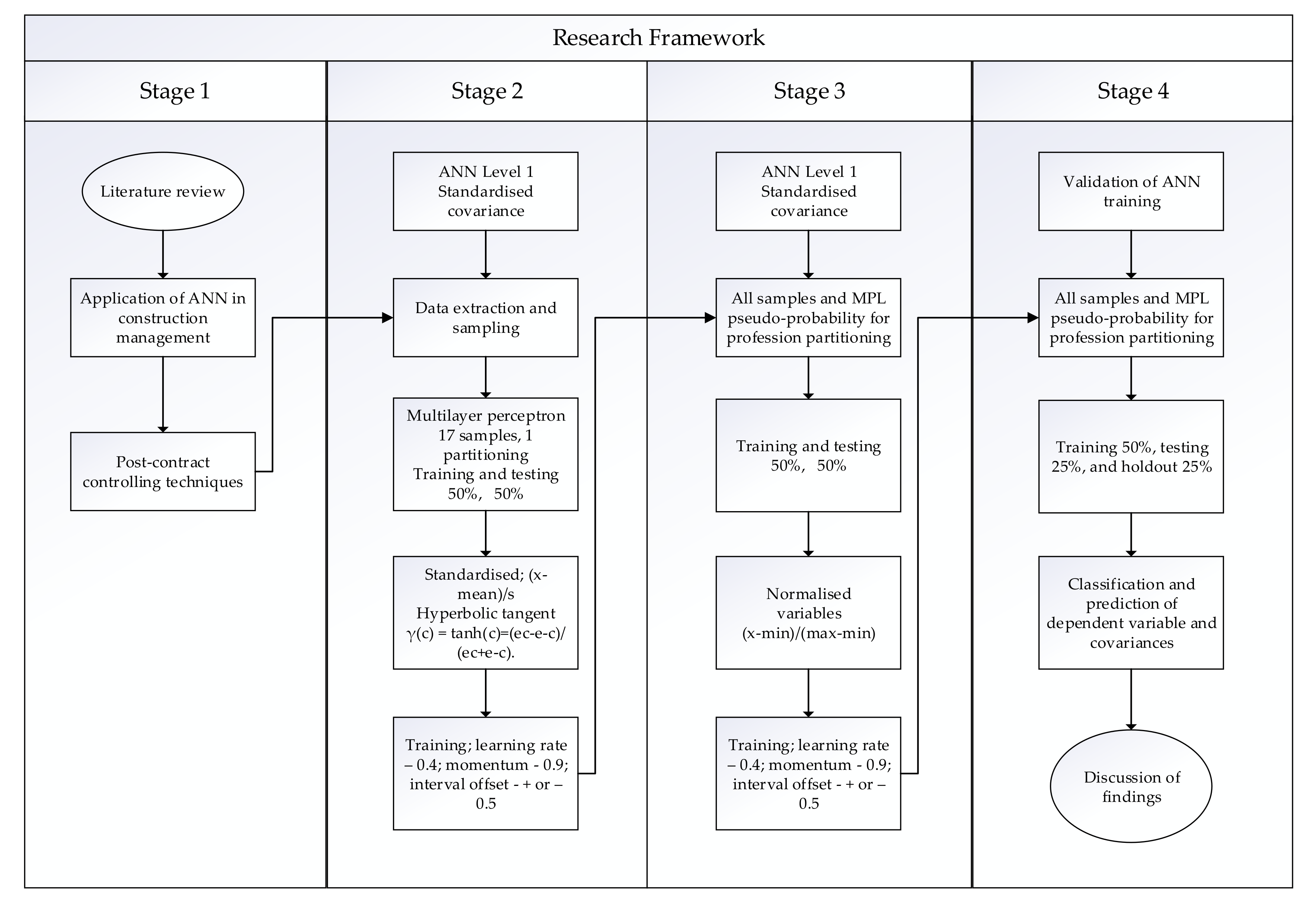
3. Research Methodology

The process of data collection and analysis in this study can be described as two-fold. In the first instance, a cross-sectional survey research design was adopted for data elicitation from a population of professionally registered QS and CPM practitioners operating in Nigeria. The choice of this research design was predicated on its flexibility, ethical advantages, efficiency, cost-effectiveness, and utility in covering geographically spread samples [69]. As such, questionnaires were distributed electronically to a cohort of pre-selected respondents. A juxtaposition of quota, purposive, and snowballing sampling techniques were deployed in identifying and recruiting respondents for this phase of the study. The respondents were drawn from the population of the database of the Quantity Surveyors Registration Board of Nigeria (QSRBN). At the point of engagement with the QSRBN database (2019), it was established that 3588 Quantity Surveyors were professionally registered and, practicing in Nigeria. Given the difficulty of identifying and accessing a similar database for CPM, it was decided to rely on data from QS professionals who had the experience of performing CPM functions on construction projects. Accordingly, respondents were asked to indicate if they had CPM experience or otherwise before engaging with subsequent sections of the questionnaire. However, this did not imply that the survey was only available for QS professionals with CPM experience. Considering the sample size of the population (3588), a margin of error of 5% and a confidence level of 95%, a total of 400 questionnaires were administered with an expectation of securing responses from at least 348 respondents. However, 135 completed responses were received from the respondents, thereby indicating a response rate of 33.75%. The minimal experience of each the respondents was over five years, and the combined linearity of the years of experience was 15 years. 54% of the respondents are QSs, and 43% of them have CPM experience in addition to their primary professional experience. At the moment, there are no Universities offering construction project management as a course and most construction project managers are from already established professions such as QS, Architecture and Building. The emphasis on CPM and QS professionals was borne out of the understanding that these professionals were mostly responsible for the determination of the post-contract cost controlling techniques to be deployed on construction sites and projects. Therefore, these professionals have a significant impact on the overall cost performance of a construction project. Consequently, the research approach extracted the data using a 5-point Likert scale. The Likert scale ratings of 1 to 5 were used to extract their perception of the importance of the post-contract cost controlling techniques. Five being highly important; 4 is important; 3, moderately important; 2, not important and 1, ignore. The second phase of this two-fold research methodology is described subsequently.

Artificial Neural Network: Multilayer Perceptron (MPL)

In this analysis, the input systems are covariances which are trained to produce an output. The QS and CPM are the primary custodians of post-contract cost controlling techniques decision making and therefore the output of the analysis.

ANN will be used to predict the most effective post-contract cost controlling technique through a pseudo-probability classification of the construction professionals in this study. The first step of this methodology extracted factors from literature sources for Likert scale data collection. The next step is level 1 ANN which adopted the standardised rescaling of the factors for the purposes of pseudo-probability. This was done to ensure that the final output is not just between the scale of 1 to 5.

The standardised rescaling used the formula:

(x − mean)/s

(1)

where x represents each value, which are subtracted from the mean of all the samples under each factor; and s is the standard deviation.

The partitioning of the data set for input was divided into training and testing. 50% of the variables were trained, and 50% were tested. The training samples served as an independent set of samples used to test the model for errors [70]. The profit and loss technique was selected as a partitioning variation in the first level because they are influenced by the remaining variables. Hence, the overall number of levels 1 training will be 17 samples instead of 18.

The hyperbolic tangent was selected as the activation function, which links the total units in one layer to another [71]. This function has the formula:

γ(c) = tanh(c)=(ec − e − c)/(ec + e − c)

(2)

γ(c) represents the hyperbolic tangent, and (ec − e − c)/(ec + e − c) connotes the direction of the synaptics.

The hyperbolic tangent collates the real-valued arguments and converts them to the range of −1 and 1. When automatic architecture selection is used, this is the activation function for all units in the hidden layers. The hyperbolic tangent is used for the output, hidden and input layers.

In stage 3 of the research framework as indicated in Figure 1, a second iteration of level 1 normalised the standardised variables using all the post-contract cost controlling factors. The multilayer perceptron output for level one was used as the new partitioning instead of profit and loss factor.

Normalisation formula involves subtracting the minimum value and then dividing it by the range, (x−min)/(max−min). Normalized values fall between 0 and 1. The learning rate for the training is given as 0.4; momentum 0.9; and offset interval is + or −0.5. The outputs of levels 1 and 2 were the pseudo-probability, classification, and normalised importance of the variables. These were all transferred to the final stage for validation using the holdout sample.

A set of holdout samples of 25% was used to validate the existing multi-trained network. In the validation stage, 50% of samples went into training and 25% was tested. The holdout samples provided an honest estimate of the predictability of the model. Therefore, identifying errors which were inconsistent in building the model. The results accruing from levels 1, 2 and the validation stage have been presented in the form of tables and graphs for clarity in the subsequent sections.

Synaptic weights represent the strength of the connections between neurons [52,70,71,72]. Iyer et al. [73] simplified synaptic weights as:

$$y_j={{\displaystyle \sum }}_i{w}_{ij }{x}_i or y=wx$$

(3)

where x is the input variable, y is the output, and the synaptic matrix represents the vector of synaptic weights for the output indexed by y_j.

The post-contract cost control variables are the neurons in this study, and the links between them are the neurons. The general rule of thumb associated neurons that fire together as wiring together. Therefore, neurons with the larger synaptic weights show stronger relations between each other.

4. Presentation and Discussion of Findings

Table 2. Network information for two training and testing sessions excluding bias.

Summary	Level 1	Level 2
Input Layer
Valid number of Samples	135	135
Number of Units	17	18
Rescaling Method for Covariates	Standardized	Normalized
Hidden Layer
Number of Hidden Layers (1)	√	√
Number of Units in Hidden (6) Layer 1	√	√
Activation Function (Hyperbolic tangent)	√	√
Output Layer
Dependent Variable (1)	√	√
Number of Units (2)	√	√
Activation Function (hyperbolic tangent)	√	√
Error Function (Sum of Squares)	16.706	29.829
Training time (sec)	2	3

(Source: Authors’ compilation, 2020)

summarised the network information for levels 1 and 2 artificial neural network training and testing. Table 2 also presents the summary of the inputs, hidden and output layers. 135 valid samples provided 17 and 18 units excluding the biases for the multilayer perceptron for Levels 1 and 2 of the research frameworks, respectively.

The sum of squares error (SSE) is 16.706% and 29.829% respectively, for levels 1 and 2. These SSE values indicate the actual error functions which are realistic for this scale of samples available. The error function for the training is averagely considerable for a predictive model. The SSE is a measure between the discrepancy between the data set and the estimated model [74,75]. Consequently, a smaller value indicates suitability.

The synaptic weights are coefficients showing the connections between the input, hidden and output layers. The training samples inform the strength of the synaptic weights even though there is a partitioning factor. The synaptic parameters in

Table 3. Synaptic parameter estimates for level 1.

Predictor		Predicted
		Hidden Layer 1						Output Layer
		H(1:1)	H(1:2)	H(1:3)	H(1:4)	H(1:5)	H(1:6)	QS	CPM
Input Layer	(Bias)	0.217	0.290	0.346	−0.143	0.535	0.025
	CFLOW	−0.303	0.107	0.487	0.057	−0.243	0.370
	HDATA	0.030	−0.661	−0.083	0.196	−0.558	−0.461
	SIMP	0.062	0.514	−0.243	0.331	−0.001	−0.187
	TCACT	0.019	0.520	−0.435	−0.102	0.144	−0.562
	MONLC	0.034	0.202	−0.395	−0.115	0.197	−0.007
	MONMC	−0.095	−0.100	−0.377	−0.481	−0.504	0.486
	MONEC	0.201	−0.882	0.183	−0.045	−0.521	−0.212
	MONOV	−0.541	0.479	−0.805	−0.505	−0.616	0.232
	VARMAN	0.653	−0.441	−0.072	0.592	0.191	−0.245
	COSTR	−0.365	0.277	0.432	0.932	−0.554	0.078
	INCMILE	−0.806	0.405	−0.124	0.501	−0.568	−0.113
	COMPUNI	−0.115	0.431	0.098	0.185	0.456	0.277
	IDCOV	−0.152	−0.071	−0.577	−0.840	0.391	0.596
	FORCOMP	0.099	−0.353	−0.690	−0.051	−0.335	−0.061
	COSTFOR	−0.338	0.381	−0.348	−0.239	−0.014	0.793
	INTERIMV	0.706	−0.094	−0.613	0.192	0.616	0.172
	WORKBUD	0.601	0.166	−0.934	−0.162	0.665	0.569
Hidden Layer 1	(Bias)							0.503	0.740
	H(1:1)							1.063	−1.063
	H(1:2)							0.565	−0.617
	H(1:3)							0.594	−0.536
	H(1:4)							−0.463	0.485
	H(1:5)							−1.046	1.069
	H(1:6)							0.421	−0.421

In the level 1, weights above 0.400 have been colour coded as MLP in the input layer synaptics leads INTERIMV; WORKBUD; INCMILE; VARMAN; MONOV largely leads mostly to H(1:1) and H(1:5). The aforementioned hidden layers links to the output layers. QS and CPM. (Source: Authors’ compilation, 2020)

are usually indicated by thicker blue or grey lines in the model. This can be in the negative or positive direction. However, the weights in

Table 4. Synaptic parameter estimates for level 2.

Predictor		Predicted
		Hidden Layer 1						Output Layer
		H(1:1)	H(1:2)	H(1:3)	H(1:4)	H(1:5)	H(1:6)	QS	CPM
Input Layer	(Bias)	0.058	−0.064	0.266	0.452	0.350	0.184
	CFLOW	0.254	0.053	0.562	0.349	0.376	0.303
	HDATA	0.527	−0.144	−0.158	−0.372	−0.261	0.195
	SIMP	0.196	0.253	−0.062	0.138	0.023	0.434
	TCACT	0.072	0.376	−0.500	0.030	−0.382	0.456
	MONLC	0.341	0.564	0.151	0.078	0.077	−0.044
	MONMC	−0.297	0.523	0.283	0.224	−0.322	0.606
	MONEC	−0.405	−0.090	0.566	−0.339	−0.402	0.667
	MONOV	−0.130	0.136	−0.098	0.196	0.326	−0.201
	VARMAN	−0.272	−0.100	−0.340	−0.322	−0.247	0.030
	COSTR	−0.146	−0.342	−0.059	0.334	0.107	−0.099
	INCMILE	−0.278	0.338	0.529	−0.627	−0.388	0.275
	COMPUNI	0.617	−0.223	−0.076	−0.034	0.058	−0.413
	IDCOV	0.381	−0.352	−0.189	0.233	0.074	0.294
	FORCOMP	0.018	−0.104	0.117	−0.098	0.126	0.275
	COSTFOR	−0.349	0.140	0.656	0.114	0.335	0.159
	INTERIMV	0.160	0.445	0.546	0.017	0.132	−0.185
	WORKBUD	0.627	0.574	−0.225	0.322	−0.107	0.056
	PampL	0.215	−0.567	0.285	−0.444	−0.235	−0.069
Hidden Layer 1	(Bias)							0.555	0.030
	H(1:1)							−0.494	0.367
	H(1:2)							0.163	−0.294
	H(1:3)							0.259	−0.198
	H(1:4)							0.527	−0.388
	H(1:5)							0.295	−0.229
	H(1:6)							0.034	0.638

(Source: Authors’ compilation, 2020).

do not entirely reflect the complete relationship between the independent or dependent variables or signify stronger association between the variables. The weights in Table 4 were presented to merely indicate the strengths of the synaptic weights.

The number of synaptic might not be used to interpret the network result if they are generally large [76]. In this study, the values of the synaptics weights will only lead us to the classification and pseudo-probability. Thus, the values in Table 3 will only be used for a preliminary mode of connecting the neurons.

From Table 4, WORKBUD; INTERIMV; INCMILE; MONEC; MONMC; and TACT largely associate with H(1:1); H(1:2); H(1:3) and H(1:6). However, H(1:1) and H(1:4) are closely linked to the QS dependent variable.

A review of the classification of the predicted dependent variables in

Table 5. Classification of predicted observed outcome from the multilayer perceptron.

Sample	Observed	QS	CPM	Percent Correct
Level 1
Training	QS	70	7	90.90%
	CPM	19	39	67.20%
	Overall Percent	65.90%	34.10%	80.70%
Level 2
Training	QS	68	9	88.30%
	CPM	38	20	34.50%
	Overall Percent	78.50%	21.50%	65.20%

(Source: Authors’ compilation, 2020).

for levels 1 and 2, signifies the QS dependent variable as 90.90% of the predictions for the post-contract cost controlling techniques. CPM is 67.20%. 80.70% of the neurons are correct for this prediction. In Level 2, 88.30% of the correct predicted outcomes are QS, and the CPM are 34.50%.

This implies that 90.90% of QS influence the decisions to choose the most influence post-contract cost controlling techniques in the first model. The first model excludes the profit and loss account. In the next model (level 2) where the profit and loss account is part of the post-contract cost controlling process, the QS has less influence on the choice of post-contract cost controlling techniques. In this model, the CPM play more role in decision making when the profit and loss account preparation is part of the process.

From Table 5, there is a confirmatory finding of who makes the most decisions to adopt a post-contract cost planning technique. The probability and pseudo-probability of who likely makes the most decisions when it comes to the choice of post-contract cost controlling techniques are crucial for overall success in the construction project.

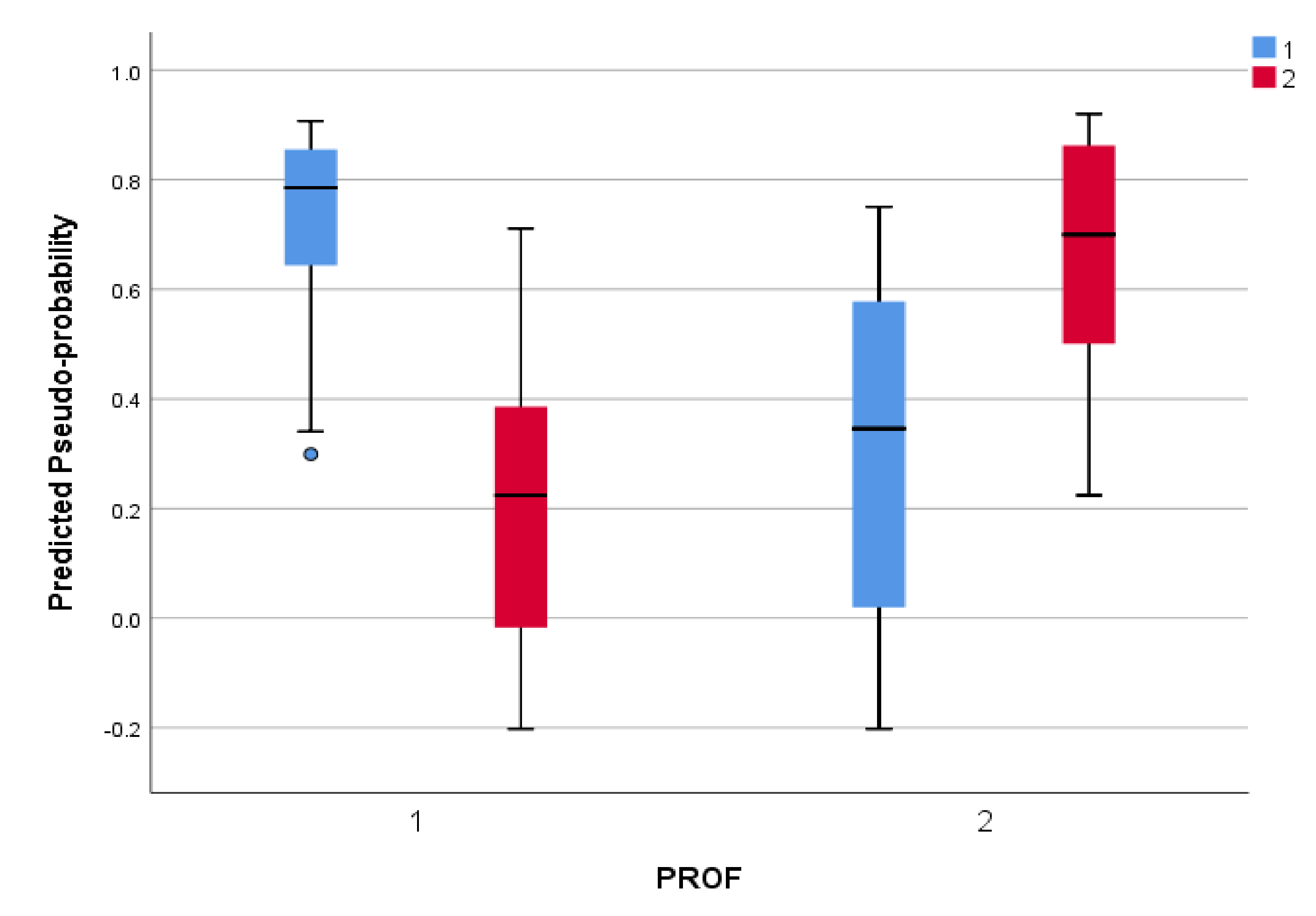
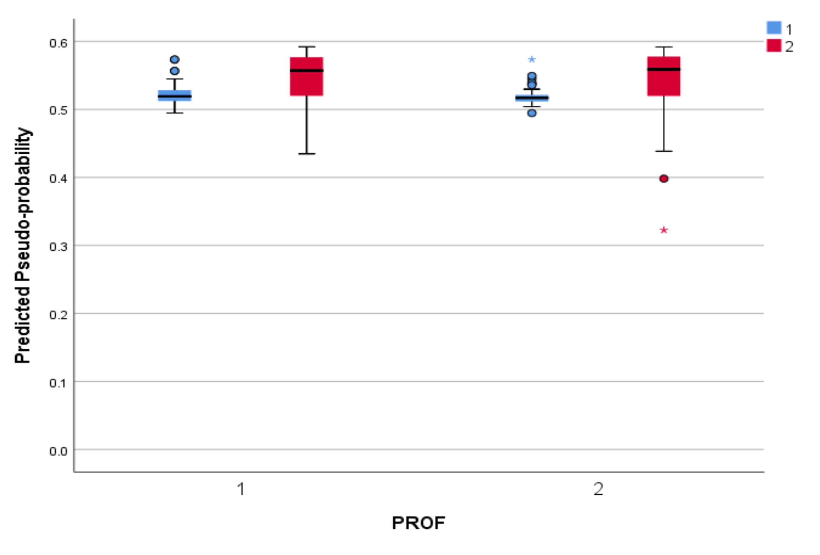
4.1. Predicted Pseudo-Probability of the Professionals

The predictive pseudo-probability of level 2 as shown in Figure 2, further confirms the findings of Table 4. Pseudo-probability is the combined likelihood of all random variables [71]. Consequently, predictive pseudo-probability further confirms the classification of the predicted output. Predictive pseudo-probability, there is further confirmation of Table 4 in a graphical format. The predictive pseudo-probability is a confirmation of the correct percentages in Table 4. Figure 3 reveals the blue box to the ‘y’ axis as values above 0.5. The blue boxes, which are also labelled as 1, represents the QS. This shows that the cases are correctly classified. The classification of 2, which is the CPM shows that the majority of the blue boxes below are below 0.5.

The predictive pseudo-probability of level 2 as shown in Figure 2, further confirms the findings of Table 4. The QS predictive percentage have a pseudo-probability which is far above 0.5 for the two categories in blue. Hence, there is a confirmation that the category of the professional output of decision making comes from the QS. This is a good result which must be validated with a holdout sample. Before the validation process, there has to be an association of variables to the classification.

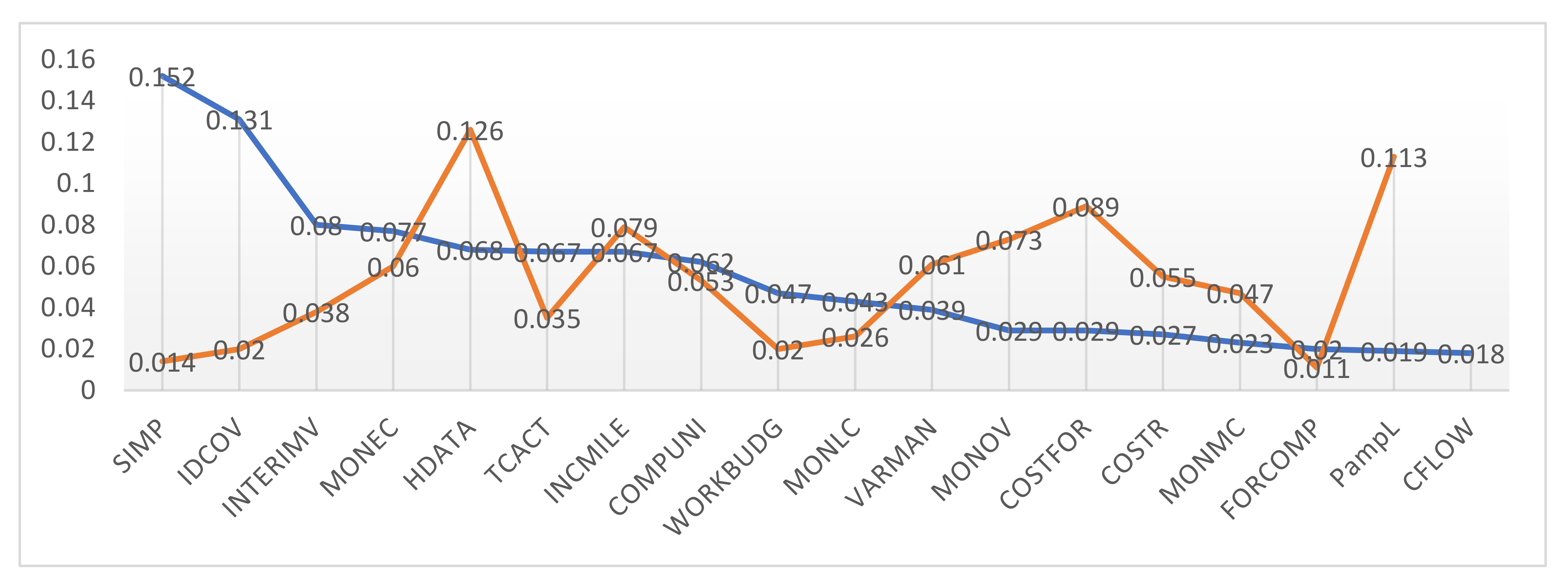
4.2. Importance of the Independent Variables

The importance of the independent variables reveals the post-contract cost controlling techniques which have more impact on the classification of outputs. The importance of the independent variables for levels 1, as indicated in

Table 6. Independent variable importance for 2 training sessions (noted: Level 1 has PampL as a partition variable in the training set).

	Level 1				Level 2
Variables	Importance	Standardised Importance	Rank	Variables	Importance	Normalised Importance	Rank
MONMC	0.087	100.00%	1	HDATA	0.126	100.00%	1
MONOV	0.086	98.40%	2	PampL	0.113	89.80%	2
MONEC	0.076	87.60%	3	COSTFOR	0.089	70.10%	3
INCMILE	0.071	82.00%	4	INCMILE	0.079	62.80%	4
VARMAN	0.069	79.40%	5	CFLOW	0.079	62.20%	5
COSTR	0.064	73.10%	6	MONOV	0.073	57.80%	6
COMPUNI	0.063	72.50%	7	VARMAN	0.061	48.50%	7
WORKBUD	0.062	71.40%	8	MONEC	0.06	47.40%	8
CFLOW	0.062	71.30%	9	COSTR	0.055	43.90%	9
IDCOV	0.061	70.50%	10	COMPUNI	0.053	42.10%	10
INTERIMV	0.05	57.70%	11	MONMC	0.047	36.90%	11
HDATA	0.05	56.80%	12	INTERIMV	0.038	30.30%	12
FORCOMP	0.049	56.00%	13	TCACT	0.035	27.70%	13
COSTFOR	0.047	54.50%	14	MONLC	0.026	20.90%	14
TCACT	0.039	44.50%	15	WORKBUD	0.02	16.20%	15
MONLC	0.032	36.50%	16	IDCOV	0.02	15.70%	16
SIMP	0.03	34.80%	17	SIMP	0.014	11.30%	17
				FORCOMP	0.011	8.70%	18

(Source: Authors’ compilation, 2020)

, clearly shows that monitoring of material cost (MONMC); variations (MONOV); equipment cost (MONEC); INCMILE and VARMAN occupy the largest percentage of the post-contract cost controlling techniques which are mostly decided by the QS.

In level 2 iteration where PampL is involved, HDATA; PampL; COSTFOR; INCMILE and CFLOW are very crucial to the QS. When there is a monthly profit and loss preparation, evidence from historical data (HDATA) and the preparation of cost forecast (COSTFOR) and cashflow registers (CFLOW) is very essential. Hence, as a building project continues, the preference for post-contract cost controlling techniques changes. The normalisation of the importance in level 2 was conducted because there is no clear indication of data distribution will behave in later stages of a construction project. In the first phase, standardised rescaling was adopted because the data had varying scales.

In the second level, the monitoring activities (MONEC, MONMC and MONMOV) have less influence in the construction project when the monthly profit and loss statements are part of the cost controls process. A validation phase towards the end of the construction project will involve all the post-contract cost controlling techniques under a normalised scenario.

4.3. Validation Using Holdout Samples

The validation of samples was conducted to finally train the model using the previously predicted outcomes of levels 1 and 2. This phase also represents the final construction stages in a project. The parameters for the input variables, which are all 135 samples are divided accordingly:

Table 7. Validation model summary.

Activity	Parameters	Values
Training	Sum of Squares Error	4.331
	Percent Incorrect Predictions	7.90%
	Stopping Rule Used	1 consecutive step(s) with no decrease in error
	Training Time	00:00.02
Testing	Sum of Squares Error	5.283
	Percent Incorrect Predictions	17.10%
Holdout	Percent Incorrect Predictions	10.70%

(Source: Authors’ compilation, 2020)

displays the model summary for the validation phase just as Figure 4 displays the connections between the nodes and variables. They are: training 50%, testing 30%, holdout sample 20% with MPL of the previous predictive value of the professionals. There are two hidden layers in the validation phase. The sum of square error for the training and testing variables are 4.331 and 5.283, respectively. The percentage of incorrect predictions for training, testing and holdout samples is 7.90%, 17.10% and 10.70% respectively. The values of the sum of squares error and incorrect predictions are considerably low enough for the validation phase of this study.

Figure 4 displays the connections between the variables and variables. The model output selected 47.4% of the training sample, 29.6% of testing and 23.0% of the holdout samples.

Table 8. Synaptic weights for normalised two hidden layers.

Predictor		Predicted
		Hidden Layer 1		Hidden Layer 2		Output Layer
		H(1:1)	H(1:2)	H(2:1)	H(2:2)	QS	CPM
Input Layer	(Bias)	0.046	0.322
	CFLOW	−0.138	0.181
	HDATA	−0.012	−0.474
	SIMP	0.452	0.360
	TCACT	−0.234	−0.174
	MONLC	−0.038	0.306
	MONMC	−0.005	0.150
	MONEC	0.422	−0.110
	MONOV	−0.210	0.299
	VARMAN	−0.261	0.086
	COSTR	−0.135	0.274
	INCMILE	0.017	0.398
	COMPUNI	0.499	−0.359
	IDCOV	0.398	0.313
	FORCOMP	0.148	−0.201
	COSTFOR	0.100	−0.286
	PampL	−0.118	0.032
	INTERIMV	0.117	0.364
	WORKBUD	0.139	0.132
Hidden Layer 1	(Bias)			0.018	0.033
	H(1:1)			−0.461	0.083
	H(1:2)			−0.505	0.424
Hidden Layer 2	(Bias)					0.575	0.222
	H(2:1)					0.318	−0.474
	H(2:2)					0.324	0.137

(Source: Authors’ compilation, 2020)

indicates the values. Site meetings and planning activities (SIMP) have a connection with H(1:1). This is consistent with monitoring equipment cost (MONEC) and the compounding unit (COMPUNI). Hidden layer H(1:2) is strongly associated with H(2:1). H(2:1) has a strong classification with the CPM.

The classification of the predicted output layer associates the SIMP; MONEC; and COMPUNI to the CPM. In

Table 9. Validated classification of predicted observed outcome from the multilayer perceptron.

Sample	Observed	Predicted
		QS	CPM	Percent Correct
Training	QS	11	26	29.7%
	CPM	8	19	70.4%
	Overall Percent	29.7%	70.3%	46.9%
Testing	QS	6	14	30.0%
	CPM	5	15	75.0%
	Overall Percent	27.5%	72.5%	52.5%
Holdout	QC	6	14	30.0%
	CPM	2	9	81.8%
	Overall Percent	25.8%	74.2%	48.4%

(Source: Authors’ compilation, 2020)

, the predicted classification of the CPM has 70.4% of the distribution for the training. The testing samples have 75% of the CPM, and the holdout validation proved 81.8% of the CPM make the most decision.

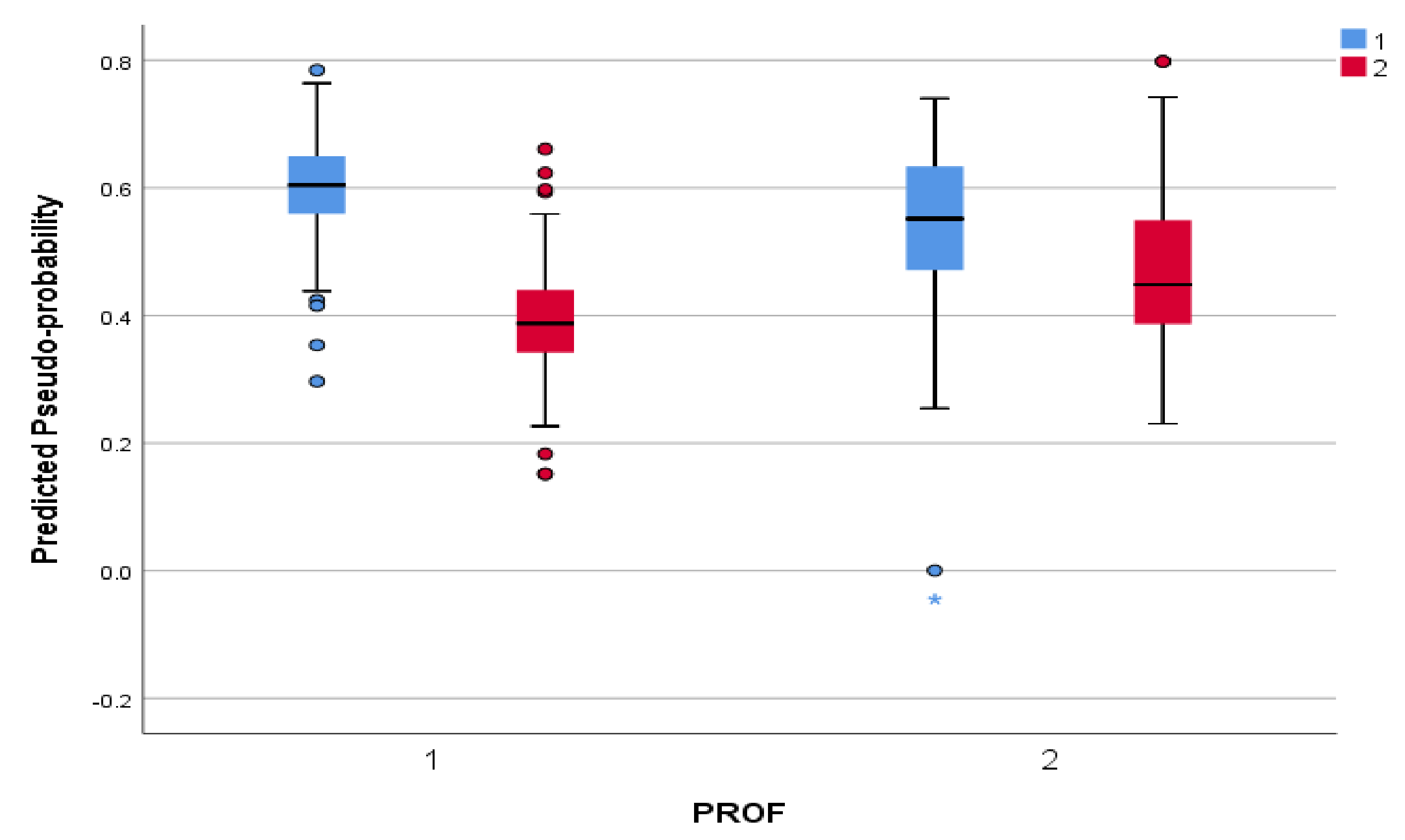
4.4. Validated Predicted Pseudo-Probability of the Professionals

The validated predicted pseudo-probability of the normalised samples reveals that all the samples are above 0.5 to the y-axis. This confirms that both the QS and CPM are involved in the decision-making process. However, the red boxes in Figure 5, shows that the CPM variables are more involved in the final phase of the decision-making process.

The validated normalised independent variables identified more of the roles the CPM plays in decision making at the end of a building construction project.

4.5. Importance of the Validated Normalised Independent Variables

The normalised variables identified site meetings (SIMP); identifying indicators of cost overrun (IDCOV); interim valuations (INTERIMV); monitoring equipment cost (MONEC) and historical (HDATA) as the main post-contract cost controlling techniques which are mostly influenced by the CPM. The abovementioned independent variables all have importance values of 0.152; 0.131; 0.080; 0.077; and 0.068 respective.

A comparison of the validated post-contract cost controlling techniques and the level 2 ranking in Figure 6, shows a chart based on

Table 10. Validated normalised importance of the post-contract cost controlling techniques.

Variable	Importance	Normalised Percentage	Rank
SIMP	0.152	100.00%	1
IDCOV	0.131	86.20%	2
INTERIMV	0.08	52.60%	3
MONEC	0.077	50.90%	4
HDATA	0.068	44.60%	5
TCACT	0.067	44.00%	6
INCMILE	0.067	44.20%	7
COMPUNI	0.062	41.00%	8
WORKBUDG	0.047	30.90%	9
MONLC	0.043	28.60%	10
VARMAN	0.039	25.70%	11
MONOV	0.029	18.80%	12
COSTFOR	0.029	18.80%	13
COSTR	0.027	17.80%	14
MONMC	0.023	15.00%	15
FORCOMP	0.02	13.30%	16
PampL	0.019	12.30%	17
CFLOW	0.018	12.10%	18

(Source: Authors’ compilation, 2020).

. In Figure 6, the x-axis is taken from the ranking in Table 10. The red line is the normalised values, while the blue line shows the values from level 2. The y-axis indicates the important values.

SIMP has a higher value in the validation when the CPM is involved in the post-contract cost controlling process. This reflects a change from 0.014 to 0.152. IDCOV is ranked second in the table with a value of 0.131 when the CPM makes most of the decisions and 0.02 when the QS is involved in choosing the post-contract cost controlling technique. INTERIMV has closer values of 0.080 and 0.038 in situations when the CPM and QS are the prime decision-makers. The values get closer for MONEC. In this variable, the CPM scenario provided a value of 0.077 and 0.060 for the QS. HDATA higher in the QS lead decision making process with a value of 0.126, while the CPM classification provided a value of 0.068.

The result of this analysis further uncovers that MONEC, INTERIMV and HDATA are often adopted by the QS and CPM in most construction projects. The least applicable techniques from the graph are the COMPUNI and MONMC. The greatest discrepancy in this analysis is the importance QS place on PampL and CFLOW during construction projects and the diminishing relevance of these post-contract cost controlling techniques to the CPM.

4.6. Reliability of Models Using Root Square Mean Error (RMSE)

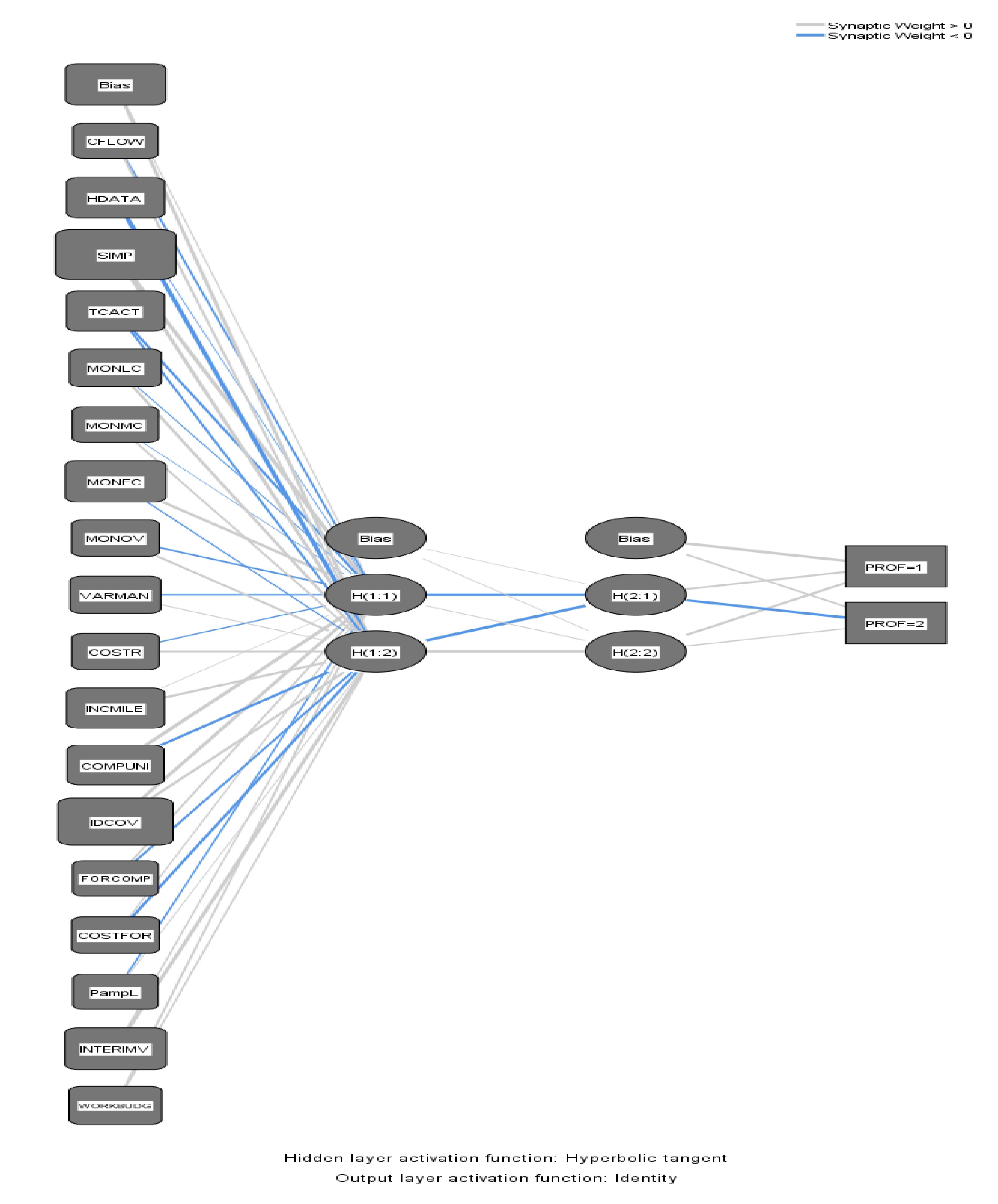
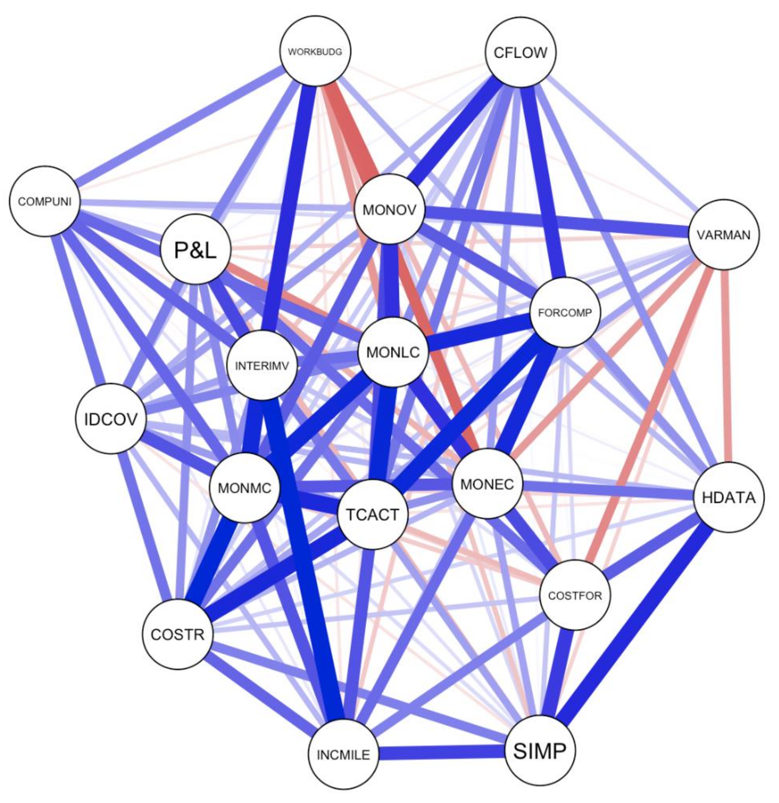
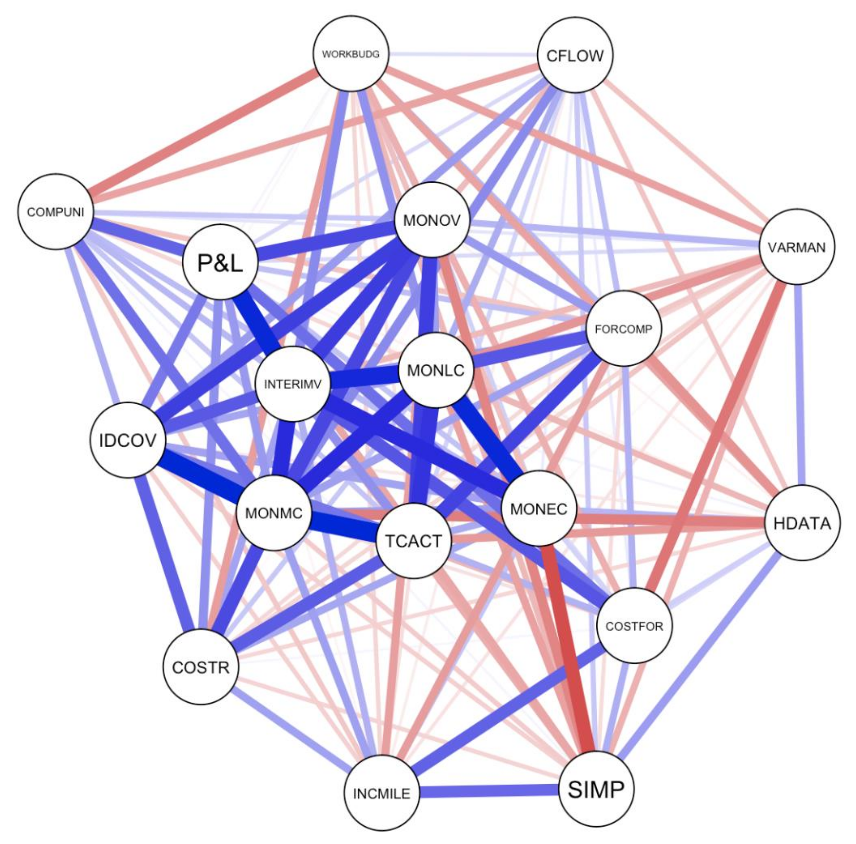
According to AgriMetSoft [76] the root square means error (RMSE) is the difference between the predicted model and observed values. The spread of the individual differences provides an aggregated predicted power of the model. The R squared values can also be used to calculate the RMSE by dividing the number of samples and then the square root of the values. The R squared values are usually between 0 and 1. The larger the R square values, the more reliable the model is. In the RMSE, the smaller values near 0 reflect absolute reliability of the model. The formula for RMSE is also given as:

$$RMSE=\frac{\sqrt{{{\displaystyle \sum }}_{i=1}^n{\left(\mathrm{XObs},\mathrm{i}-\mathrm{Xmodel},\mathrm{i}\right)}^2}}{\mathrm{n}}$$

(4)

where X(Obs,i) is the observation value and X(model,i) is the forecast value.

The RMSE for the models in level 1, 2 and validation are indicated below.

Table 11. R square and RMSE values.

Level	N	R SQUARE	RMSE
1	135	0.308	0.048
2	135	0.725	0.073
Validation	135	0.726	0.073

(Source: Authors’ compilation, 2020)

displays the various models, levels 1, 2 and validation, the number of samples, R squared and RMSE values for each model.

The R square value for the first level excluded the monthly profit and loss statements and was able to predict 30.8% of the independent variables. The RMSE indicates a value of 0.048, thus, providing a very good fit for the model. An enhanced study with the multilayer perceptron dependent variable in level 2 and validation provided R square values of 72.5% and 72.5% of the independent variables. They provide an excellent RMSE fit of 0.073 for both levels. The RMSE value of 0.073 proves that the predictions are very reliable.

4.7. Network Model

Nykamp [77] opined that a network is a collection of nodes connected to each other with links. When the sizes of the edges are weighted in a matrix, it is denoted by thicker lines [77]. Network diagrams mimic synaptics in a brain and are used to illustrate the strength of relationships between nodes. The synaptics from the artificial neural network within a brain wave format can be linked together to create a network.

Table 12. Summary of the network.

Network	Number of Nodes	Number of Non-Zero Edges	Sparsity
QS	18	153/144	0.000
CPM	18	153/144	0.000

(Source: Authors’ compilation, 2020)

summarised the network diagram in Figure 7 and Figure 8. There are 18 nodes representing post-contract cost control and 153 links for all 18 post-contract cost controlling techniques out a possible 144 links. The sparsity value of 0 indicates a very sparse and less dense network, thereby indicating linearity of the nodes. Hence, the closer the value is to 0, the sparser the network is. This is a good indication of linearity in the network. The network diagram shows the darker blue lines as the positive links between the nodes and the red lines are the negative connections within the network. The relevant post-contract cost controlling techniques are also larger in the network. The smaller nodes specify less relevance. For instance, there is a negative connection between the working budget (WORKBUDG) and monitoring equipment cost (MONEC). This is realistic because equipment costs are not prepared in the bill of quantities by the QS.

The network plot for the QS in Figure 7, shows the connection between taking corrective action (TCACT); monitoring labour cost (MONLC); monitoring material cost (MONMC); cashflows (CFLOW). Site meeting and post-project reviews are very relevant to the QS and it is associated strongly with historical data (HDATA), incremental milestones and cost forecasting (COSTFOR). The CPM network plot in Figure 8, clearly shows a strong relationship between Monitoring material cost (MONMC); labour cost (MONLC) and equipment cost (MONMC) along with interim valuations (INTERIMV). The CPM also thinks that site-meeting and post-project reviews are important. However, monitoring equipment cost (MONEC) is very difficult for the CPM to management, hence, the bold red line in the network.

A comparison of the QS and CPM network plots revealed that there are more negative (red) connections in the CPM plot compared to the QS. The negative connections in the CPM network plot is an indication of a lack of understanding of how post-contract cost controlling techniques work. Hence, the QS must be the primary influencer of the type of post-contract cost controlling techniques that will be adopted at every construction stage. The next sections discuss the implication of the findings, limitation of the study and conclusions, which will lead to further studies.

5. The Implications of Results

At various stages of construction, new decisions are made to keep the project within the expected objectives. The results from this study have addressed post-contract cost controlling techniques from the QS and CPM perspective. Levels 1, 2 and validation were taken respectively as the initiation phase of construction cost control; mid-point of the construction; and final stages of construction. Levels 1 and 2 also connotes, the training phases before the validation of the model.

5.1. Levels 1 and 2

From the classification Table 5, 90.9% and 88.3% of QSs make the most decisions to select a post-contract cost controlling technique. Table 6 also predicts monitoring material cost (MONMC) historical data (HDATA) have the highest normalised importance of 100% to the QS. In level 1, the use of the terminology ‘monitoring’ connotes that some construction activities cannot be controlled but monitored. However, by monitoring the material cost, inflations, payments, the sub-contractors and suppliers, there will be more an opportunity to keep the project within budget at the earlier stages which are usually the facilitating works and substructure.

At Level 2, which represents the mid-point of construction, another set of post-contract cost controlling techniques become more sacrosanct. From the findings, the QS has more need to control the cost. Thus, the need for historical data (100%), cost forecasting (70.1%), cash flows (62.8%) and profit and loss statements (62.8%) will suffice. From recent studies into cost overruns, cost control has been studied as a valid influence [23,24]. This implies that further studies, into more stages of building construction, may expose differing behavioural tendencies towards construction cost control among stakeholders.

The network model of Figure 6 further confirms the normalised importance of the techniques to the QS. Monitoring material cost (MNMC) is associated with labour cost, equipment cost; and taking corrective action. The similarity between QS and CPM network model is the site meeting and post-project reviews which relate to historical data.

5.2. Validation: Towards the End and after Construction

Towards the end of the construction phase, the CPM has been predicted to have more stake in the decision-making process when it comes to cost control by a value of 81.8%. Hence, the need for more site meetings and post-project reviews (100%); identification of cost overrun indicators (86.2%); interim valuations (52.6%) and historical data (44.6%). The results are linked to the network model of Figure 7 which revealed that site meeting and post-project reviews are closely linked to historical data and identifying cost overruns have links to interim variations and monitoring material cost and taking corrective action. This is from the perspective of the CPM’s thinking.

Interim valuations are a common post-contract cost controlling techniques across level 2 and the final validation phase. According to Ashworth and Perera [14], interim valuations entails valuations of a construction project at stages or specified intervals. Interim evaluations are connected to monthly statements and the profit and loss accounts. The profit and loss account statement is also linked to cashflow registers or cost forecasting. At the end of every construction project, there is a need to review the project though post-project evaluation and assess the profit and loss account.

The implication of the findings of this study is that the QS should be more involved in decision-making as it pertains to the choice of post-contract cost controlling techniques at every state in construction. In terms of cost control, the techniques adopted by the QS are different from the CPM. Consequently, there is a need to understand construction cost management and how different stakeholders influence decisions during construction. Further studies into how other stakeholders influence the choice of post-contract cost controlling techniques will engender a strengthening of collaborations between the construction stakeholders whilst enhancing a reduction of disputes occurrence.

6. Limitations of this Study

This study has only addressed the backward prediction of the type of post-contract cost controlling techniques QS and CPM may adopt in construction. The data set used in this analysis is also smaller than the usual big data analysis, a case study using larger sample size can be used in the future with this methodological approach. The outcome of the artificial neural network reveals how classification of QS and CPM at different stages in a project perform under a network analysis. Future work will need to further validate the findings with on-site case data. Future studies may address other construction stakeholders who may influence the adoption of specific post-contract cost controlling techniques based on case scenarios. Other modern techniques such as intranet-based cost control, BIM 5D and other non-traditional cost controlling measures were not included. The justification for this limitation stems from the cross-sectional nature of the study and the source of the primary data, which is Nigeria. Traditional cost controlling techniques are still in force in Nigeria and in many developing countries. Consequently, the analysis and results of this study are confirmatory in nature.

7. Conclusions

The aim of this study was to propose a structured decision-support methodology for predicting the most applicable PCCTs using ANN. Eighteen (18) post-contract cost controlling techniques were identified through literature search and their applicability in practice was obtained from QSs and CPM through a questionnaire survey in the Nigerian construction industry. The ANN outputs had three iterations taken at the initial phase of construction, mid-level, and the close-out phases, respectively. The ANN analysis provided normalised importance of the post-contract cost controlling techniques. At the initial phase, the results of the multilayer perceptron show that 90.9% of QS will normally combine monitoring of material, equipment, and overhead cost. In the mid-level phase, the results show that 88.3% QS will use historical data along with profit and loss statements, cost forecasting and cash flow registers. It is concluded that the QS is the primary decision maker for the type of PCCTs at the initial and middle phases of construction project delivery. In the closing out phase of a project, the ANN output classified 81.8% of the CPM as the primary decision-maker. It is concluded that the CPM is the primary decision maker for the type of PCCTs at the closing phase of construction project delivery. The CPM at the final stages of construction adopts site meeting and post-project reviews; identification of cost overruns; interim valuations and historical data. As a construction project progresses, the CPM influences the decision-making process and thus, the post-contract cost controlling techniques adopted. Furthermore, the network plot reveals more interactions between the post-contract cost controlling techniques for the QS and fewer associations for the CPM. The conclusion is that the QS has the greater involvement and influence than the CM in the decision making for selecting post-contract cost controlling techniques for construction project delivery.

The innovation of this study are as follows. The ANN has been presented as method for analyzing cross-sectional survey data to predict the decision making of construction professionals in choosing the PCCTs in different phases in construction project delivery. The standardised rescaling of operationalised variables for pseudo-probability demonstrates how data collected using the questionnaire can be adapted for ANN analysis. Furthermore, this study shows that the decision making on PCCTs covers three distinct phases of construction project delivery (initial phase, mid-level phase and closing phase) and that the influence of the decision makers differs across the phases. This study presents the stages where QS and CPM are influential in ensuring that the right PCCTs are selected for successful project delivery and client satisfaction.

References

1. Jugdev, K.; Müller, R. A retrospective look at our evolving understanding of project success. Proj. Manag. J. 2005, 36, 19–31. [Google Scholar] [CrossRef]
2. Munns, A.K.; Bjeirmi, B.F. The role of project management in achieving project success. Int. J. Proj. Manag. 1996, 14, 81–87. [Google Scholar] [CrossRef]
3. Radujković, M.; Sjekavica, M. Project management success factors. Procedia Eng. 2017, 196, 607–615. [Google Scholar] [CrossRef]
4. Khodeir, L.M.; El Ghandour, A. Examining the role of value management in controlling cost overrun [application on residential construction projects in Egypt]. Ain Shams Eng. J. 2019, 10, 471–479. [Google Scholar] [CrossRef]
5. Petheram, C.; McMahon, T. Dams, dam costs and damnable cost overruns. J. Hydrol. X 2019, 3, 100026. [Google Scholar] [CrossRef]
6. Pinheiro Catalão, F.; Cruz, C.O.; Sarmento, J.M. Exogenous determinants of cost deviations and overruns in local infrastructure projects. Constr. Manag. Econ. 2019, 37, 697–711. [Google Scholar] [CrossRef]
7. Love, P.E.; Sing, M.C.; Ika, L.A.; Newton, S. The cost performance of transportation projects: The fallacy of the Planning Fallacy account. Transp. Res. Part A Policy Pract. 2019, 122, 1–20. [Google Scholar] [CrossRef]
8. Pilger, J.D.; Machado, Ê.L.; de Assis Lawisch-Rodriguez, A.; Zappe, A.L.; Rodriguez-Lopez, D.A. Environmental impacts and cost overrun derived from adjustments of a road construction project setting. J. Clean. Prod. 2020, 2020, 120731. [Google Scholar] [CrossRef]
9. Cunningham, T. Cost Control during The Construction Phase of the Building Project: The Consultant Quantity Surveyor’s Perspective; Dublin Institute of Technology: Dublin, Ireland, 2017. [Google Scholar]
10. Potts, K.; Ankrah, N. Construction Cost Management: Learning from Case Studies; Routledge: London, UK, 2014. [Google Scholar]
11. Omotayo, T.; Kulatunga, U. A continuous improvement framework using IDEF0 for post-contract cost control. J. Constr. Project Manag. Innov. 2017, 7, 1807–1823. [Google Scholar]
12. Monyane, G.; Emuze, F.; Awuzie, B.; Crafford, G. Evaluating a Collaborative Cost Management Framework with Lean Construction Experts. In Proceedings of the The 10th International Conference on Engineering, Project, and Production Management, Berlin, Germany, 2–4 September 2019; Springer: Singapore, 2020. [Google Scholar]
13. Ahsan, K.; Ho, M.; Khan, S. Recruiting project managers: A comparative analysis of competencies and recruitment signals from job advertisements. Project Manag. J. 2013, 44, 36–54. [Google Scholar] [CrossRef]
14. Ashworth, A.; Perera, S. Cost Studies of Buildings; Routledge: London, UK, 2015. [Google Scholar]
15. Olawale, Y.A.; Sun, M. Cost and time control of construction projects: Inhibiting factors and mitigating measures in practice. Constr. Manag. Econ. 2010, 28, 509–526. [Google Scholar] [CrossRef]
16. Cartlidge, D. Construction Project Manager’s Pocket Book; Routledge: London, UK, 2015. [Google Scholar]
17. Oyeyipo, O.; Odusami, K.T.; Ojelabi, R.A.; Afolabi, A.O. Factors affecting contractors’ bidding decisions for construction projects in Nigeria. J. Constr. Dev. Ctries. 2016, 21, 21–35. [Google Scholar] [CrossRef]
18. Igwe, U.S.; Mohamed, S.F.; Azwarie, M.B.M.D.; Paulson Eberechukwu, N. Recent Developments in Construction Post Contract Cost Control Systems. J. Comput. Theor. Nanosci. 2020, 17, 1236–1241. [Google Scholar] [CrossRef]
19. Abobakr, A. Necessity of Cost Control Process (Pre & Post Contract Stage) in Construction Projects: Cost Control in Pre & Post Contract. MSc Thesis, University of Applied Sciences, Berlin, Germany, 2018. [Google Scholar]
20. Sanni, A.; Durodola, O. Assessment of contractors’ cost control practices in Metropolitan Lagos. In Proceedings of the Procs 4th West Africa built Environment Research (WABER) Conference, Abuja, Nigeria, 24–26 July 2012. [Google Scholar]
21. Mac-Barango, D. Cost Control Systems and Good Governance: Tools for Effective Project Delivery. Int. J. Econ. Financ. Manag. 2017, 2, 29–44. [Google Scholar]
22. Omotayo, T.; Kulatunga, U. Re-Thinking Post-Contract Cost Controlling Techniques in the Nigerian Construction Industry. In Proceedings of the 5th World Construction Symposium: Greening Environment, Eco Innovations and Entrepreneurship, Colombo, Sri Lanka, 29–31 July 2016. [Google Scholar]
23. Kern, A.; Soares, A.; Formoso, C. Introducing target costing in cost planning and control: A case study in a Brazilian construction firm. In Proceedings of the CIB W107 Construction in Developing Countries International Symposium-“ Construction in Developing Economies: New issues and Challenges”, Santiago, Brazil, 18–20 January 2006. [Google Scholar]
24. Fedorova, N.V.; Shaforost, D.A.; Bundikova, V.R.; Denisova, I.A. Some aspects of functional modeling in the IDEF0 standard as the initial stage of TPPs design. AIP Conf. Proc 2019, 2188, 050010. [Google Scholar]
25. Presley, A.; Liles, D.H. The use of IDEF0 for the design and specification of methodologies. In Proceedings of the 4th Industrial Engineering Research Conference, Nashville, TN, USA, 24–25 May 1995. [Google Scholar]
26. Oladapo, M. A framework for cost management of low-cost housing. In Proceedings of the International Conference on Spatial Information for Sustainable Development, Nairobi, Kenya, 2–5 October 2001. [Google Scholar]
27. Akintoye, A.S.; Ajewole, O.; Olomolaiye, P.O. Construction cost information management in Nigeria. Constr. Manag. Econ. 1992, 10, 107–116. [Google Scholar] [CrossRef]
28. Corbett, P.; Rowley, P. The use of BCIS elemental cost data by quantity surveyors as part of cost planning techniques: The practitioners’ perspective. In Proceedings of the 15th Annual ARCOM Conference, Liverpool John Moores University, Liverpool, UK, 15–17 September 1999. [Google Scholar]
29. Robson, A.; Boyd, D.; Thurairajah, N. Studying ‘cost as information’ to account for construction improvements. Constr. Manag. Econ. 2016, 34, 418–431. [Google Scholar] [CrossRef]
30. Sanni, A.; Hashim, M. Assessing the challenges of cost control practices in Nigerian construction industry. Interdiscip. J. Contemp. Res. Bus. 2013, 4, 366–374. [Google Scholar]
31. Aliverdi, R.; Naeni, L.M.; Salehipour, A. Monitoring project duration and cost in a construction project by applying statistical quality control charts. Int. J. Project Manag. 2013, 31, 411–423. [Google Scholar] [CrossRef]
32. Kubba, S. Handbook of Green Building Design and Construction: LEED, BREEAM, and Green Globes; Butterworth-Heinemann: Oxford, UK, 2012. [Google Scholar]
33. Al-Jibouri, S.H. Monitoring systems and their effectiveness for project cost control in construction. Int. J. Project Manag. 2003, 21, 145–154. [Google Scholar] [CrossRef] [Green Version]
34. Al-Hazim, N.; Salem, Z.A.; Ahmad, H. Delay and cost overrun in infrastructure projects in Jordan. Procedia Eng. 2017, 182, 18–24. [Google Scholar] [CrossRef]
35. Bolhassani, B.; Hovorka, S.D.; Hosseini, S.A.; Young, M.H.; Anderson, J.S.; Yang, C. Model-based assessment of the site-specific cost of monitoring. Energy Procedia 2017, 114, 5316–5319. [Google Scholar] [CrossRef]
36. Moser, R.; Narayanamurthy, G.; Kusaba, K.; Kaiser, G. Performance of low-cost country sourcing projects–Conceptual model & empirical analysis. Int. J. Prod. Econ. 2018, 204, 30–43. [Google Scholar]
37. Jeong, H.; Sun, A.Y.; Zhang, X. Cost-optimal design of pressure-based monitoring networks for carbon sequestration projects, with consideration of geological uncertainty. Int. J. Greenh. Gas Control 2018, 71, 278–292. [Google Scholar] [CrossRef]
38. Martens, A.; Vanhoucke, M. The impact of applying effort to reduce activity variability on the project time and cost performance. Eur. J. Oper. Res. 2019, 277, 442–453. [Google Scholar] [CrossRef] [Green Version]
39. Odeck, J.; Kjerkreit, A. The accuracy of benefit-cost analyses (BCAs) in transportation: An ex-post evaluation of road projects. Transp. Res. Part A Policy Pract. 2019, 120, 277–294. [Google Scholar] [CrossRef]
40. Oliveira, R. Monitoring and Control of Schedule and Cost Performance in Facade Conservation. Procedia Struct. Integr. 2019, 22, 151–159. [Google Scholar] [CrossRef]
41. Cavalieri, M.; Cristaudo, R.; Guccio, C. On the magnitude of cost overruns throughout the project life-cycle: An assessment for the Italian transport infrastructure projects. Transp. Policy 2019, 79, 21–36. [Google Scholar] [CrossRef]
42. Çelik, T.; Arayici, Y.; Budayan, C. Assessing the social cost of housing projects on the built environment: Analysis and monetization of the adverse impacts incurred on the neighbouring communities. Environ. Impact Assess. Rev. 2019, 77, 1–10. [Google Scholar] [CrossRef]
43. Peñaloza, G.A.; Saurin, T.A.; Formoso, C.T. Monitoring complexity and resilience in construction projects: The contribution of safety performance measurement systems. Appl. Ergon. 2020, 82, 102978. [Google Scholar] [CrossRef]
44. Construction Industry Institute. Control for Construction; Construction Industry Institute: Texas, TX, USA, 1987. [Google Scholar]
45. Czernigowska, A. Earned value method as a tool for project control. Bud. Archit. 2008, 3, 15–32. [Google Scholar]
46. Verma, A.; Pathak, K.; Dixit, R. Earned value analysis of construction project at Rashtriya Sanskrit Sansthan, Bhopal. Int. J. Innov. Res. Sci. Eng. Technol. 2014, 3, 11350–11355. [Google Scholar]
47. Puvanasvaran, A.; Kerk, S.; Ismail, A. A case study of kaizen implemention in SMI. In Proceedings of the National Conference in Mechanical Engineering Research and Postgraduate Studies, UMP Pekan, Pahang, Malaysia, 3–4 December 2010. [Google Scholar]
48. Okoye, P.V.C.; Egbunike, F.C.; Meduoye, O.M. Product cost management via the kaizen costing system: Perception of Accountants. J. Mgmt. Sustain. 2013, 3, 114. [Google Scholar]
49. Sanchez, F.; Steria, S.; Bonjour, E.; Micaelli, J.P.; Monticolo, D. An approach based on bayesian network for improving project management maturity: An application to reduce cost overrun risks in engineering projects. Comput. Ind. 2020, 119, 1066–3615. [Google Scholar] [CrossRef]
50. Sarbayev, M.; Yang, M.; Wang, H. Risk assessment of process systems by mapping fault tree into artificial neural network. J. Loss Prev. Process Ind. 2019, 60, 203–212. [Google Scholar] [CrossRef]
51. Zainuddin, N.H.; Lola, M.S.; Djauhari, M.A.; Yusof, F.; Ramlee, M.N.A.; Deraman, A.; Ibrahim, Y.; Abdullah, M.T. Improvement of time forecasting models using a novel hybridization of bootstrap and double bootstrap artificial neural networks. Appl. Soft Comput. 2019, 84, 1568–4946. [Google Scholar] [CrossRef]
52. Bewes, J.; Low, A.; Morphett, A.; Pate, F.D.; Henneberg, M. Artificial intelligence for sex determination of skeletal remains: Application of a deep learning artificial neural network to human skulls. J. Forensic Legal Med. 2019, 62, 40–43. [Google Scholar] [CrossRef]
53. Ok, S.C.; Sinha, S.K. Construction equipment productivity estimation using artificial neural network model. Constr. Manag. Econ. 2006, 24, 1029–1044. [Google Scholar] [CrossRef]
54. Attalla, M.; Hegazy, T. Predicting cost deviation in reconstruction projects: Artificial neural networks versus regression. J. Constr. Eng. Manag. 2003, 129, 405–411. [Google Scholar] [CrossRef]
55. Ogunlana, S.O.; Sdhabhon, B. Application of artificial neural network to forecast construction duration of buildings at the predesign stage. Eng. Constr. Archit. Manag. 1999, 6, 133–144. [Google Scholar]
56. Bhosale, A.; Konnur, B. Use of Artificial Neural Network in Construction Management. Int. J. Innov. Eng. Sci. 2019, 4, 73–76. [Google Scholar]
57. Waziri, B.S.; Bala, K.; Bustani, S.A. Artificial neural networks in construction engineering and management. Int. J. Arch. Eng. Constr. 2017, 6, 50–60. [Google Scholar] [CrossRef]
58. StackExchange. What is the difference between estimation and prediction? 2011. Available online: https://stats.stackexchange.com/questions/17773/what-is-the-difference-between-estimation-and-prediction (accessed on 20 January 2020).
59. Goh, Y.M.; Chua, D. Neural network analysis of construction safety management systems: A case study in Singapore. Constr. Manag. Econ. 2013, 31, 460–470. [Google Scholar] [CrossRef]
60. Sodikov, J. Cost estimation of highway projects in developing countries: Artificial neural network approach. J. East. Asia Soc. Transp. Stud. 2005, 6, 1036–1047. [Google Scholar]
61. Jha, K.N.; Chockalingam, C. Prediction of schedule performance of Indian construction projects using an artificial neural network. Constr. Manag. Econ. 2011, 29, 901–911. [Google Scholar] [CrossRef]
62. Wilmot, C.G.; Mei, B. Neural network modeling of highway construction costs. J. Constr. Eng. Manag. 2005, 131, 765–771. [Google Scholar] [CrossRef]
63. Lam, K.C.; Ng, S.T.; Tiesong, H.; Skitmore, M.; Cheung, S.O. Decision support system for contractor pre-qualification—artificial neural network model. Eng. Constr. Archit. Manag. 2000, 7, 251–266. [Google Scholar]
64. Shan, M.; Le, Y.; Yiu, K.T.; Chan, A.P.; Hu, Y.; Zhou, Y. Assessing collusion risks in managing construction projects using artificial neural network. Technol. Econ. Dev. Econ. 2018, 24, 2003–2025. [Google Scholar] [CrossRef]
65. Li, H.; Love, P.E. Combining rule-based expert systems and artificial neural networks for mark-up estimation. Constr. Manag. Econ. 1999, 17, 169–176. [Google Scholar] [CrossRef]
66. Mirahadi, F.; Zayed, T. Simulation-based construction productivity forecast using neural-network-driven fuzzy reasoning. Autom. Constr. 2016, 65, 102–115. [Google Scholar] [CrossRef]
67. Shan, M.; Le, Y.; Yiu, K.T.; Chan, A.P.; Hu, Y.; Zhou, Y. Application of artificial neural network (s) in predicting formwork labour productivity. Adv. Civil Eng. 2019, 2019, 1–11. [Google Scholar]
68. Arafa, M.; Alqedra, M. Early stage cost estimation of buildings construction projects using artificial neural networks. Early Stage Cost Estim. Build. Constr. Proj. Using Artif. Neural Netw. 2011, 4, 63–75. [Google Scholar] [CrossRef] [Green Version]
69. Owens, L.K. Introduction to survey research design. SRL Fall 2002 Seminar Series, 1 January 2002. [Google Scholar]
70. Roman, N.D.; Bre, F.; Fachinotti, V.D.; Lamberts, R. Application and characterization of metamodels based on artificial neural networks for building performance simulation: A systematic review. Energy Build. 2020, 2020, 109972. [Google Scholar] [CrossRef]
71. International Business Machine (IBM). IBM Neural Networks 19; SPPS: Sussex, UK, 2010. [Google Scholar]
72. Yu, Y.; Qu, Y. Multi-component spectral detection based on neural network in water quality inspection. Optik 2020, 2020, 164915. [Google Scholar] [CrossRef]
73. Iyer, R.; Menon, V.; Buice, M.; Koch, C.; Mihalas, S. The influence of synaptic weight distribution on neuronal population dynamics. PLoS Comput. Biol. 2013, 9, e1003248. [Google Scholar] [CrossRef] [Green Version]
74. Kharin, V.V.; Zwiers, F.W. On the ROC score of probability forecasts. J. Clim. 2003, 16, 4145–4150. [Google Scholar] [CrossRef]
75. Fawcett, T. An introduction to ROC analysis. Pattern Recognit. Lett. 2006, 27, 861–874. [Google Scholar] [CrossRef]
76. AgriMetSoft. RMSE (Root Mean Square Error). 2019. Available online: https://agrimetsoft.com/calculators/Root%20Mean%20Square%20Error (accessed on 4 June 2020).
77. Nykamp, D. An introduction to networks. 2020. Available online: https://mathinsight.org/network_introduction (accessed on 4 January 2020).
Figure 1. Research framework for ANN prediction of post-contract cost controlling techniques in building construction (Source: Authors’ compilation, 2020)
Applsci 10 05171 g001
Figure 2. Predictive pseudo-probability for the level 1 training.
Applsci 10 05171 g002
(Source: Authors, 2020)
Figure 3. Predictive pseudo-probability of the second level.
Applsci 10 05171 g003
Figure 4. Validated multilayer perception.
Applsci 10 05171 g004
Figure 5. Validated predicted pseudo-probability for the professionals.
Applsci 10 05171 g005
Figure 6. A comparison of the normalised importance for level 2 and validate independent variable.
Applsci 10 05171 g006
Figure 7. Network plot for quantity surveyor.
Applsci 10 05171 g007
Figure 8. Network plot for CPM.
Applsci 10 05171 g008