On the Synergy between Elemental Carbon and Inorganic Ions in the Determination of the Electrical Conductance Properties of Deposited Aerosols: Implications for Energy Applications

Featured Application

Results presented in this work demonstrated that the elemental carbons have a role in the formation of electrical bridging phenomena in synergy with hygroscopic aerosol components. Applications are related to filtering systems in free cooled data centers and cleaning protocol (e.g., for high power level insulators) able to remove the elemental carbon hydrophobic element and not only the hydrophilic compounds to avoid shorts and failures.

Abstract

The role of the elemental carbon (EC), in synergy with hygroscopic ionic species, was investigated to study the formation of electrical bridging phenomena once the aerosol deliquescence is achieved. Ambient aerosol samples were collected on hydrophobic surfaces in urban and rural sites in Northern Italy; their conductance was measured in an Aerosol Exposure Chamber (AEC) while varying the relative humidity. An electric signal was detected on 64% of the collected samples with conductance values (11.20 ± 7.43 μS) above the failure threshold (1 μS) of printed circuit boards. The ionic content was higher for non-electrically conductive samples (43.7 ± 5.6%) than for electrically conductive ones (37.1 ± 5.6%). Conversely, EC was two times higher for electrically conductive samples (26.4 ± 4.1 μg cm⁻²; 8.4 ± 1.7%) than for non-electrical ones (12.0 ± 4.1 μg cm⁻²; 5.2 ± 1.9%) suggesting that the synergy between the ionic and carbonaceous fractions is necessary to promote a bridging phenomenon. Synthetic aerosols (EC only, saline only, mixed saline and EC) were generated in laboratory and their conductance was measured in the AEC to verify the ambient results. Only in case of a contemporary presence of both EC and ionic components the bridging phenomenon occurred in keeping with the theoretical deliquescence values of each salt (R² = 0.996).

1. Introduction

The physical state (wet or dry) of atmospheric aerosols determines their physical–chemical properties responsible for their behavior in various environmental processes, such as atmospheric corrosion and bridging phenomena [1,2,3,4,5], interaction with solar radiation and satellite applications [6,7,8,9,10,11] as well as heterogeneous reactivity on the aerosol’s surface [12]. The critical points of the phase transition of an atmospheric particle are the deliquescence and the crystallization relative humidity (DRH and CRH). DRH and CRH determine whether in certain atmospheric conditions aerosol particles are solid or liquid (i.e., their soluble components are in solution) in function of the variation of the relative humidity (RH) of the surrounding atmosphere. Particularly, starting from a RH < DRH, the aerosol is dry until RH reaches DRH; from this point the aerosol absorbs water producing a saturated aqueous solution. Any other RH increase leads to a continuous condensation of water (hygroscopic growth). Conversely, a reduction in RH (starting from a value above DRH) leads to evaporation until the CRH is reached promoting the aerosol crystallization and bringing again the aerosol to a dry state [13,14,15,16]. The DRH and the CRH depend on the chemical composition of the aerosol itself and on the ambient temperature [11,13,14,17]. The aforementioned cycle is known as hysteresis cycle of the aerosol [14,18,19].

Among many fields of interest, the aerosol hydration state is relevant for energy applications related to energy distribution and electronic reliability [18,20,21]. They concern both outdoor and indoor environment. In the first case, an example of outdoor exposed components is represented by insulators of high voltage (HV) transmission lines. Transmission lines are used for transmission of electric power and their continuous operation is essential for the reliability of power grid. Insulators are a relevant part of the system, because of their role in isolation of conductors from the tower and mechanical support for the line. Insulator performance is commonly affected by several factors: material, shape, degradation and pollution [22,23]. The last one, combined to atmospheric conditions, plays a relevant role in failures: hygroscopic aerosol particles, such as saline deposits layers, mostly cause flashover during their water-soluble state [24,25,26]. In fact, it is well known that an insulating surface, placed between two electrodes and moistened with atmospheric agents (dew, rain, fog, etc.), reduces its dielectric strength [27]. This phenomenon increases when soluble pollution species dissociate in ions, acquiring conductive characteristics. The consequence is a disruptive discharge over insulator surface [28,29,30] which finally turns into energy distribution failures and financial consequences for the energy distributor.

On the other hand, aerosols conductivity (in function of RH) also represents a central issue in indoor contexts. Hereinafter, the term “indoor” is used in its broader meaning describing any confined environment, ranging from an Information Technology room to a case (of any electronic device) installed outdoors. With respect to this, atmospheric aerosols can penetrate indoor [20,31] and when hydrated, could represent a potential danger for the indoor installed electronic components [32,33,34,35], since they can induce three main effects on electronics [36]. First of all, electrochemical corrosion can occur and the impact of the deposited aerosols can be different if ionic species are in the solid state or are dissolved [1,4,5,37]. In addition, particles deposited on electronics can have mechanical effects, such as heat accumulation on electronic circuitry, or electrical effects. For example, electrical bridging phenomena could be caused by particles deposited between components that would normally be electrically insulated in a printed circuit [38,39]. In addition, according to the percolation theory [40], the aerosol loading has to exceed a critical surficial concentration value in order to create a continuous conductive path. A further factor that affects electrical bridging caused by deposited particles is that the conductance of aerosols can be different as a function of their physical state. If the aerosol particles are hydrated (i.e., over the DRH with increasing RH or over the CRH if RH is decreasing from above the DRH) the ionic components spontaneously dissolve, creating a conductive electrolytic solution. Therefore, hygroscopic particles can potentially originate conductive paths and cause electrical leakage [41]. Consequently, in literature, hygroscopic aerosol is believed to be the major responsible for printed circuit boards (PCBs) failures [1,38,39,42,43].

The aerosol induced failures in indoor environment are also extremely connected with energy consumption. In recent studies, Ferrero et al. [18,20] performed aerosol conductance measurements in function of RH in order to set-up safe thermodynamic ranges for the electronic equipment installed indoor in “green” Free-Cooled Data Centers to avoid any failure. Green Free-Cooled Data Centers consists of data centers in which outdoor air is used to cool the information technology equipment (i.e., high-performance calculators) within a data center. However, traditionally, in order to avoid any corrosion and failure, data centers cool the hot air produced by the information technology using air-conditioning units through a closed-loop air cycle also drying the recycled air. This approach is responsible for a ~35–50% of energy consumption in a data center just for the cooling process [33,34,44]. As a result, data centers are responsible for more than 2% of worldwide electricity consumption [45]. In an alarmist scenario, Andrae and Edler [46] suggested that the global power demand of data centers could reach as much as 13% of global electricity use in 2030, corresponding to a 14-fold increase compared with the 1.1 to 1.5% of the global electricity use, in 2010 [47]. However, Andrae [48] revised this value to 3% in 2025. Ferrero et al. [18,20] demonstrated that a safe use (i.e., avoiding ions deliquescence) of the Free-Cooling approach (which avoid the air-conditioning usage) leads to an energy saving up to 80% of the cooling process allowing to avoid the emissions of tens of ktons of CO₂ and other absorbing material into the atmosphere. This is beneficial also in a climate change mitigation perspective [49,50]. In this respect, it is well-known that aerosol components other than the ionic inorganic fraction are hygroscopic, consequently be involved in this kind of phenomena [51,52]. Examples are carboxylic acids and other organic compounds classes [53,54,55,56,57,58]. Most important, it has been demonstrated that even non-electrolyte substances (e.g., sucrose) can induce a deterioration of PCB components [59].

Among the non-electrolyte substances, the elemental carbon (EC) could play a significant role. Briefly, elemental carbon indicates carbonaceous particles deriving from combustion processes and composed of graphene layers with small contents of heteroatoms, especially oxygen and hydrogen [60,61,62]. Often the term “soot” is improperly used as a synonymous of elemental carbon especially when laboratory flame carbonaceous material is generated. Here this term is introduced as it was proven that flame generated soot can be electrically conductive [63], even if the measured conductivity values (between 10⁻⁶ and 10⁻² Ω⁻¹ cm⁻¹, depending on the sample density and on the fuel used for soot production) could be lower than those of pure graphite (between 10⁻³ and 10⁻¹ Ω⁻¹ cm⁻¹, depending on the sample density). This is caused by the mainly disordered and amorphous structure of soot: in effect, unlike pure graphite that has just hybrid sp2 C atoms and valence electrons in the remaining π-orbital, flame soot contains also some sp3 bonds [60,64]. Accordingly, supposing that soot could play a role in electrical bridging processes caused by aerosols deposited on electronics seems reasonable.

Despite the huge amount of aforementioned literature, up to now, to the authors’ knowledge, the synergy between ionic components and other common atmospheric aerosol conductive species (e.g., the elemental carbon) in the formation of electrical bridges was never investigated. Tencer et al. [39] discussed the surficial critical ionic density in promoting a bridging effect while Ferrero et al. [18] determined the surficial critical aerosol density (127 ± 7.8 μg cm⁻²) to observe it. The threshold of 127 μg cm⁻² corresponds to an ambient concentration of PM_2.5 of 27.5 μg m⁻³ (considering the filtering area of PM_2.5 filter samples) which in Milan for example is exceeded more than ~70% of time in winter and just ~34% of all days throughout the year. No information is available on the role of EC with respect to the aforementioned barrier.

Therefore, the aim of this work is to investigate the role that EC, in synergy with hygroscopic saline species, has in the formation of electrical bridging phenomena promoted by deposited aerosol particles on hydrophobic surfaces, simulating the high voltage insulator and printed circuit boards (PCBs) surfaces.

At this purpose, aerosol samples were collected on PTFE (Teflon) in different environments (urban and rural site), in Northern Italy (Po Valley). The investigated sites are located in the Po Valley, a hotspot for atmospheric pollution [65] where the dry aerosol deposition rate ranges from 30 to 70 μg cm⁻² month⁻¹ [66] making the aerosol a potential dangerous material for energy application. Moreover, the two urban and rural sites were chosen as affected by different EC and ionic content [67].

The collected samples were examined measuring their conductance in an Aerosol Exposure Chamber in function of the relative humidity (RH) meanwhile the inorganic ionic and EC content of each sample was analyzed. In addition to field measurements, laboratory experiments, with generation of synthetic aerosol were conducted. Pure saline, pure EC and externally mixed EC and saline aerosols were generated and collected on hydrophobic supports; their conductance during humidity cycles was measured as well.

All the obtained conductance measurements are discussed in relation to the quantified ionic and EC content in the context of two significant energy application in the Italian territory: maintenance of the insulators of high-voltage transmission lines and green data centers geared with Direct Free-Cooling.

2. Materials and Methods

This section describes the main features of the methodological approach followed to determine the synergy between the EC and the hygroscopic saline species in promoting the formation of electrical bridging phenomena at different RH.

At this purpose, Section 2.1 describes the aerosol sampling in different environments (urban and rural sites). Section 2.2 is dedicated to the aerosol chemistry determination while conductance measurements (as a function of RH) are detailed in Section 2.3. Finally, Section 2.4 describes the generation of synthetic aerosol either saline-inorganic or EC; their conductance during humidity cycles was measured as well.

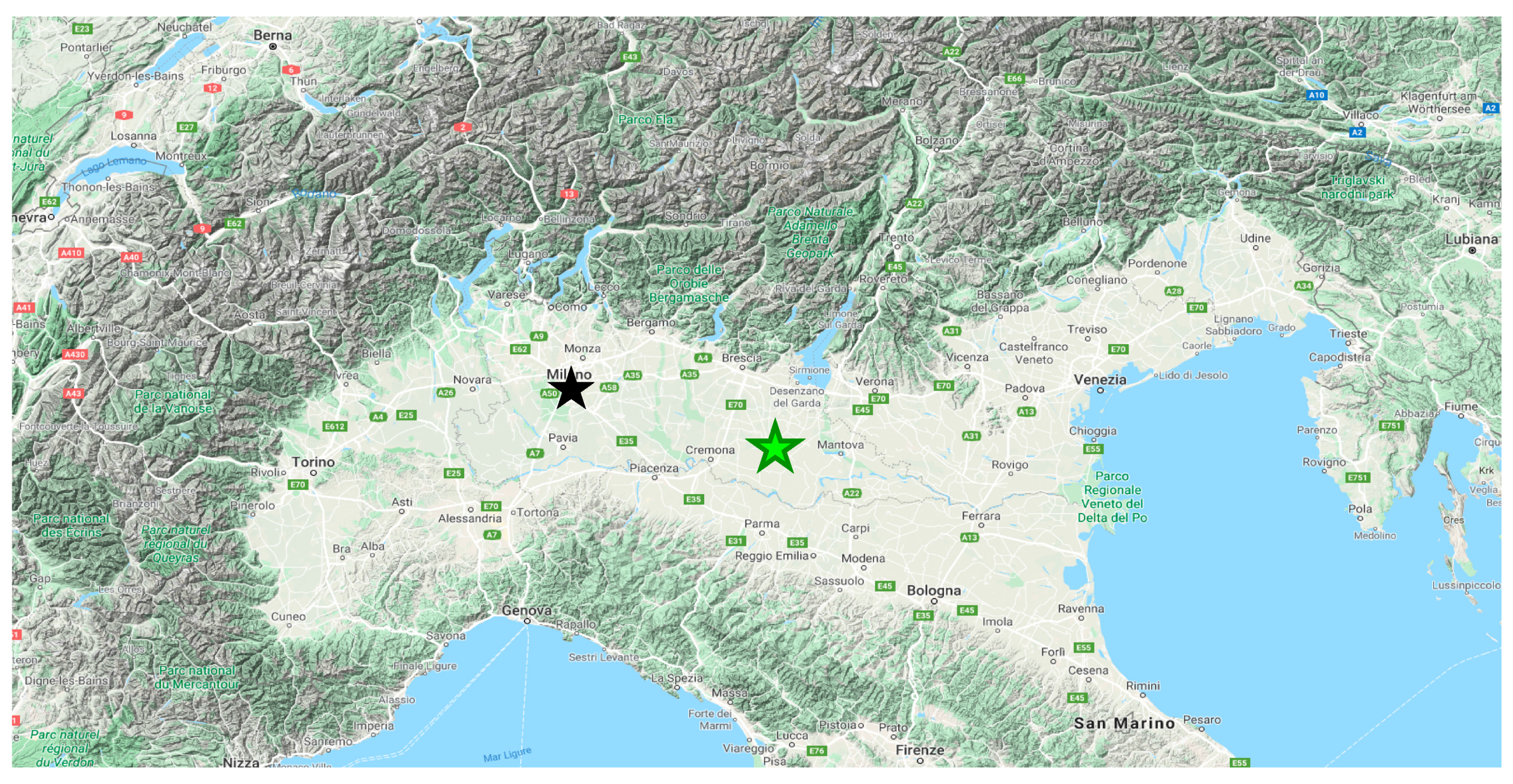
2.1. Aerosol Sampling

The aerosol samples were collected choosing the PM2.5 as a reference standard. This choice is supported by previous studies [18,20,33,68] in which it has been demonstrated that this fine aerosol fraction is capable of getting into a data center despite the presence of an industrial filtering system (MERV13). Moreover, as it has been shown in other studies [19,69] PM_2.5 represents an important fraction of the aerosol involved in the deposition mechanism occurring on vertical surfaces such as the high voltage transmission lines insulators. In this respect, fine aerosol particles (i.e., PM_2.5) have a long residence time and are able to reach high altitudes as PM vertical profiles in the Po Valley demonstrated [6,70,71]. Thus, PM_2.5 particles are also able to reach the electric line insulators making the choice of PM_2.5 reliable for the purpose of the present study.

PM_2.5 samples were collected in accordance with the EN-14907 standard on both PTFE (Ø = 47 mm, PTFE, PALL R2PJ047, 2.0 µm porosity with a retention of 1 and 2 µm particle size of 99.99% and 3 µm particle size of 99,79%) and quartz fiber filters (Ø = 47 mm, Whatman QM-A, 2.2 µm nominal porosity, 99.999% filtration efficiency) for 24 h with a FAI-Hydra Dual Channel Low-Volume-Sampler (2.3 m3 h-1 flow rate). PM_2.5 samples were collected at the Milan ‘Torre Sarca’ sampling site (MI-TS, 45°31′19″ N, 9°12′46″ E) and at the rural site of ‘Oasi Le Bine’ (OB, 45°8′17.24″ N 10°26′10.99″ E) from 2005 to 2009. Figure 1 presents the location of the two PM_2.5 sampling sites (MI, urban and OB, rural), which are characterized by a different chemical composition (Section 3.2) and are located in the Po Valley (a European atmospheric pollution hot spot) [71,72,73,74] due to the frequent stable atmospheric conditions which favors pollutant accumulation. A full description of these sampling sites and the characterization of aerosol properties (chemical composition, vertical profiles, sources and toxicity) for both MI-TS and OB sites was published by Ferrero et al. [7,70,73], Perrone et al. [67], Sangiorgi et al. [75]. Here we just underline that all the collected samples were stored at −18 °C in dark conditions in the Filters Bank of the University of Milano Bicocca. This Filters Bank has the purpose of storing PM samples in safe conditions for later analysis and investigations on new aspects of the research on aerosols. For the aims of this work, comparing aerosol samples from different sampling sites was important, since their different mean chemical compositions result in different electrical behaviors (Section 3.2). The number of samples considered in this work together the season of sampling are detailed in Section 3.2 and Supplementary Material (Table S1).

PTFE filters were chosen because they are among the most common membranes for aerosol collection, thanks to their low blank values for ions they are a suitable matrix for ion chromatography analysis [76] (Section 2.2); in addition, previous studies [8,18,19,77] demonstrated that hydrophobic supports are the most suitable for aerosol-water interaction measurements (e.g., via conductance measurements). In addition, their hydrophobicity makes them a good surrogate [66] for hydrophobic surfaces, e.g., epoxy-based composites that constitute PCBs and circuit component encapsulates [78] and for glass/ceramic insulator material, making them a good candidate for the present study. Quartz fiber filters were used to determined elemental and organic carbon as detailed in Section 2.2.

PTFE filters were cut exactly in two halves, so that it was possible to perform ion chromatography analysis (Section 2.2) and conductance measurements in the AEC (Section 2.3) on two equal portions of the same sample. In this respect, the homogeneity of PM samples on filters was assessed in a previous study [79]. Moreover, any mechanical artefact was avoided using a specific Teflon Cylinder which keep the filter locked during a guillotine cut performed by a pre-cleaned stainless steel cutter (Figure S1, Supplementary Materials). The method was validated along more ten years of research on PM (e.g., Ferrero et al., [18] and reference therein) and also validated in Aerosol Exposure Chamber measurements when comparing the hygroscopic responses and conductance of the two halves [8,80].

2.2. Aerosol Chemical Characterization

PM chemical composition was determined at TS-MI and OB sites. A coupled ion chromatography system (Dionex ICS-90 and ICS-2000) was used to analyze the ionic inorganic fraction [6,81]. For ion chromatography analysis, samples were extracted in 3 mL of ultrapure water (Milli-Q Water; resistivity of 18.2 MΩ∙cm at 25 °C) with a 20 min ultrasonic bath. Prior to analysis, the obtained solutions were filtered (0.45 μm PTFE membrane, 15 mm Syringe Filters, Phenomenex), in order to remove any possible solid particle in suspension. The characterization of the ionic fraction was performed by means of the ICS2000 and ICS90 coupled ion chromatography systems (Dionex) equipped with an AS3000 Autosampler. Anions (F⁻, Cl⁻, NO3⁻, SO₄²⁻) were separated with Dionex AG14A-5μm and AS14A-5μm Guard and Analytical columns in an isocratic run of Na₂CO₃/NaHCO₃ (concentration 8.0 mM/1.0 mM, Dionex) at a flow rate of 0.5 mL min⁻¹. The electrical signal of the eluent was lowered by means of a chemical suppressor (Dionex AMMS III 2 mm MicroMembrane Suppressor, regenerant solution: H₂SO₄, 0.05 M, Fluka 84720). Cations (Na⁺, NH₄⁺, K⁺, Ca²⁺, Mg²⁺) were separated with CG12A-5 μm and CS12A-5 μm Guard and Analytical columns by means of an isocratic run of MSA (methanesulfonic acid, CH₃SO₃H, 20 mM, Fluka 64280) at a flow rate of 0.5 mL/min. In this case too, the signal of the eluent was decreased with a chemical suppressor (Dionex CMMS III 4 mm MicroMembrane Suppressor, regenerant solution: tetrabutylammonium hydroxide, TBA-OH, 0.1 M, Fluka). Elemental and organic carbon (EC and OC) were determined using a Thermal Optical Transmission method (TOT, Sunset Laboratory inc.; NIOSH 5040 procedure; [82,83]). The chemical methods as well as the main results of the chemical analysis were yet validated and published [7].

2.3. Conductance Measurements

The determination of the conductance in function of RH, and thus the determination of both DRHs and CRHs of the collected aerosol samples was performed in a specifically designed Aerosol Exposure Chamber (AEC) [8,18,19]. The AEC is a sealed 1 m³ glass chamber in which the collected aerosol samples are exposed to humidification and dehumidification cycles, from 30 to 90% RH and vice versa, with RH steps of 1%. The RH is varied inside the chamber by introducing either dry or moist pure air in it (Aria Zero, Sapio), while the temperature is kept constant at 25 °C (the fixed temperature cooling of the Free-Cooling data center, see Ferrero et al. [18,20]). Temperature and relative humidity were monitored by means of a thermo-hygrometric sensor (DMA672 coupled with an ELO008 Data-Logger, LSI-Lastem, ±1% RH and ± 0.1 °C accuracy) during the whole cycle. As reported in D’Angelo L. [80], equilibration tests were performed monitoring the electrical response and RH with 30 min step each within the AEC in order to observe the time needed to reach the equilibrium in conductance measurements. Figure S2a (Supplementary Materials) shows a typical equilibration time experiment. During 30 min, the RH conditions resulted to be constant with a fluctuation of less than 0.5% RH and this produced a constant electrical response (Figure S2a, Supplementary Materials). However, whenever RH exhibit small variations (e.g., in Figure S2b,c at 56% and 58% RH) the electrical conductance followed RH in perfect agreement (R² = 0.915). Moreover, Figure S3 reports conductance for each RH steps at 0 s, 180 s, 1200 s and 1800 s for the sample showed in Figure S2a. As the conductance was constant and reached very fast (i.e., seconds) the equilibration, the conductance measurements were carried out waiting two minutes after that the RH reached the target value to avoid any random fluctuations. As a result, each experiment (humidification and dehumidification) lasted ~4 h.

Within the AEC, up to 6 aerosol samples can be housed at a time in specifically-designed PTFE filter holders, each provided with a pair of electrodes that allowed the measurement of the electrical resistance of the deposited aerosol at each RH step. The electrodes were set at a fixed calibrated distance of 5 mm (a balance between inter soldier parts on PCB board, size of PTFE filters) and the electrical measurements were performed with a 3421A Data Acquisition Unit (Hewlett-Packard, 0–30 MΩ measured resistance range). With respect to the electrodes, any influence of their mechanical pressure applied to samples is negligible as previously demonstrated [80]. This result was obtained by measuring via AEC the conductance signal on the same PM_2.5 sample (collected on PTFE filters) a second time. In this respect an example of a sample exposed to two RH cycles is reported in Figure S4 (Supplementary Materials): the profiles highlighted a good repeatability (R² = 0.99, slope = 1.032) of the measurements.

During the humidification phase, the hygroscopic components of the aerosol samples promote water uptake and a steep increase in the samples’ conductance can be observed in correspondence to the deliquescence of water-soluble compounds, because of the formation of a conductive electrolytic solution. On the contrary during dehumidification, when a strong decrease in conductance is measured, the crystallization of water-soluble compounds occurs. Thus, DRH and CRH values of each sample can be determined in correspondence to the maximum conductance gradient in the humidification and dehumidification curves respectively, according to the method reported by Ferrero et al. [18] and validated in D’Angelo et al. [8]. A typical plot of the measured conductance as a function of the RH applied in the chamber is shown in Section 3.1. Their determination in a sample implies that the whole ensemble of aerosol chemical composition deposited onto the filter concurred, in synergy, to an electrical bridging at a certain RH. In this respect, the minimum aerosol mass surficial loading for these kinds of measurements (127 ± 7.8 μg cm⁻²) has been first determined in Ferrero et al. [18] (to which we refers) and the factors affecting it are discussed in the present paper in Section 3.2 as they are strictly connected to synergy between EC and ionic fractions in promoting bridging and other failures on electronic devices.

2.4. Laboratory Generated EC and Saline Aerosols

In order to investigate the role of EC in promoting the aerosol conductance, different aerosol types (soot only, saline only, externally mixed saline and soot) were generated in the laboratory.

First of all, soot particles were generated from an acetylene non-premixed diffusion flame. Acetylene was produced from a controlled reaction between ultrapure water and calcium carbide. The generated acetylene was gurgled in ultrapure water in order to prevent any particle or solid contaminant to reach the flame. In addition, the gurgler avoids any possible backfire to the acetylene generation unit. The flame was constantly kept at a height of 5 cm and the generated soot was sampled by means of a glass cone placed above the flame itself for 20 s and injected into a 50 L PTFE chamber. As the aim of the paper is to investigate the role that the EC has (in synergy with hygroscopic saline species) on the aerosol conductance, the chemical-physical features of the generated soot were characterized. First of all, the generated soot was analyzed with a Thermal Optical Transmission method (TOT, Sunset Laboratory inc.; NIOSH 5040 procedure) to quantify the elemental and organic carbon (EC and OC) content (Section 2.2); the measured EC percentage on the total carbon content (TC) was determined on five soot samples: it was on average 95.2 ± 2.5%. This indicates a low content of organic matter and is in agreement with what found in literature for acetylene flame soot [84,85] reaching the highest level compared to industrial soot generators [86]. Too deepen the chemical investigation, the same samples were analyzed with gas chromatography (Agilent 6850, mass spectrometer 5973) according to the method described by Pietrogrande et al. [87] for the quantification of polycyclic aromatic hydrocarbons (PAHs) and n-alkanes (C20-C32) as organic carbon matter, in order to verify the low content of organic species found with TOT measurements. On average, 104 ± 62 pg of PAHs were quantified per μg of soot mass while the content of n-alkanes was 305 ± 184 pg μg⁻¹. If these amounts are compared with the average concentrations of PAHs and n-alkanes measured in atmospheric aerosols at the MI-TS site (PAHs from 100 to 600 pg μg⁻¹, n-alkanes in the 800–3000 pg μg⁻¹ range, annual ranges; [88]) the PAHs and n-alkanes content in the laboratory generated soot samples is either much lower with what found in atmospheric aerosols. In addition to its chemical characterization, the number size distribution of the generated soot was determined by means of an SMPS 3936 (Scanning Mobility Particle Sizer Spectrometer, TSI Inc.) and it was found to be bimodal, with the two maximums at 68 nm and 250 nm, respectively (Figure S5, Supplementary Material).

Finally, the generated EC conductance was also measured within the AEC in dry conditions (30% RH) for eight soot samples (3 to 20 μg cm⁻² deposited on a PTFE filter). The measured conductance was in the 20–180 μS range at 30% RH, which is comparable to what measured for the soot from a gas turbine engine by Popovicheva et al. [63].

In order to investigate the synergy between EC and inorganic ions, pure saline aerosols were generated by means of the Aerosol Generator ATM 220 (Topas GmbH) from aqueous solutions. Four salts were investigated, namely: ammonium sulfate (AS: (NH₄)₂SO₄), ammonium nitrate (AN: NH₄NO₃), ammonium chloride (AC: NH₄Cl), sodium chloride (SC: NaCl) and sodium sulfate (SS: Na₂SO₄). Among them, special attention was given to (NH₄)₂SO₄ and NH₄NO₃, since they are among the most abundant inorganic species found in the Po Valley atmospheric aerosols; in this respect, as their relative abundances reflect their Winter and Summer concentrations in the Po Valley [7,88], winter-like aerosol (WI-mix) and summer-like saline (SU-mix) aerosol were also generated. They were composed of 24% (NH₄)₂SO₄ + 76% NH₄NO₃ (WI-mix) and of 86% (NH₄)₂SO₄ + 14% NH₄NO₃ (SU-mix). The starting solutions were prepared at a concentration of 2.5 × 10⁴ ppm, in order to achieve satisfactory particles concentrations according to the manufacturer specifications for the Aerosol Generator. The concentration was always the same for all solutions, and when a mix is used, the reported concentration was the total of all components. The number size distribution of the generated aerosol was characterized with the TSI SMPS, too (monomodal, 50–80 nm range peak, Figure S5, Supplementary Material).

First of all, pure saline samples were generated and they were exposed to humidification and dehumidification cycles in the AEC (Section 2.3). At a later stage, EC and saline aerosols were generated simultaneously into two different Sampling Chambers (50 L volume each, TEFLON^® FEP type 200 A, thickness 50 μm), as shown in the schematic in Figure 2. All the generated aerosols were collected on PTFE filters (Ø = 47 mm, 2 μm porosity) by means of a pump (Leland Legacy, SKC, 15 L/min flow). In order to obtain well externally-mixed generated aerosol samples, the two flows from the two Sampling Chambers were conveyed through a three-ways glass connector, which couples the two sampling flows before they get to the filtering PTFE membrane. In order to avoid contamination between two consecutive aerosol generation experiments, the two Sampling Chambers were cleaned with a pure air flow for five times their volume.

SMPS data were collected at the inlet of the PTFE filter holder to be representative of the real size distribution deposited onto the PTFE filters (average residence time of particles into the chambers: 6.7 min). Finally, the cake deposits were characterized as reported in literature [89,90,91] from SMPS data determining first the a-dimensionless Peclet number (Pe) and the following cake porosity (ε) as detailed in Thomas et al. [91]:

$$Pe=\frac{Uf{d}_{agg}}{D}$$

(1)

$$\epsilon =\frac{1+0.44Pe}{1.019+0.46Pe}$$

(2)

where Uf is the filtration face velocity, d_agg, the aggregated or agglomerated particle size (SMPS data, Figure S5, Supplementary Materials) and D, the particle diffusion coefficient. In the present case, even the PTFE filters were of 47 mm diameter, the PMP ring reduced the active size spot to a 39 mm diameter (11.94 cm²; Figure S6, Supplementary Materials); thus, considering a sampling flow rate of 15 l min⁻¹ this translate into a Uf of 0.21 m s⁻¹. D was calculated from d_agg according to the Stokes–Einstein equation [92]. The ε determined using the Thomas et al. [91] method enables to account for the non-linearity over a wide range of Pe.

From the cake porosity and the cake mass per surface area (m_s) the deposit thickness ΔZ can be computed as follows [90,91]:

$$\Delta Z=\frac{m_s}{(1 - \epsilon ){\rho }_p}$$

(3)

where ρ_p is the material density.

The aforementioned calculations were used to discuss the obtained results in Section 3.3. Similarly to the atmospheric aerosol samples, also these soot and saline aerosols were exposed to humidification and dehumidification cycles. The results of these measurements are presented and discussed in Section 3.3 while Table S2 (Supplementary Materials) reports the aerosol mass deposited and composition for all synthetic samples.

3. Results and Discussion

Conductance and chemical analysis on samples collected at the urban site of MI-TS and at the rural site OB are first presented in Section 3.1 and Section 3.2, respectively; the aim is to highlight the different electrical behavior in function of the ionic and EC content presents on ambient aerosol samples in different sites. Section 3.3 presents the results obtained from laboratory generated aerosol samples in order to confirm the results obtained from MI-TS and OB samples. All the data along the manuscript text, within tables and figures are reported as mean ± confidence interval at 99% (α = 0.01).

3.1. Measured Conductance

Starting with ambient measurements, 62 samples were characterized and exposed to RH cycles in the AEC for the determination of their DRHs and CRHs together with their conductance. 50 of them were collected at the urban site of MI-TS and 12 at the rural site OB (sampling activity in OB was conducted on a shorter period compared to MI-TS). The mass distributions on filter for MI-TS samples varied from 74.8 μg cm⁻² to 496.8 μg cm⁻², while the samples from the OB site presented surficial mass distributions from 100.0 μg cm⁻² to 184.4 μg cm⁻². These are typical values for the Po Valley, which is characterized by seasonally modulated pollution [72]. As previously reported in Ferrero et al. [18] a first estimation of the minimum aerosol loading to observe an electric conduction gave the value of 127 ± 7.8 μg cm⁻². In this respect, considering the whole ensemble of the investigated PM2.5 samples, a subset of 42 samples gave a detectable electrical signal in function of RH, representing 68% of the collected samples.

Thus, in order to deepen the critical factors of the aerosol chemical composition affecting the aerosol conductivity (in an energy application perspective; next section), here below conductance measurements carried out on PM2.5 samples in the AEC are first investigated focusing on the electric signal behavior in function of RH changes.

Figure 3 shows a typical electrical conductance measurement on a PM_2.5 sample as a function of RH applied in the AEC during both humidification and dehumidification. DRH and CRH values together with the deliquescence and crystallization regions can be individuated according to the conductance derivative [18] (Section 2.3). As a case study, a winter sample was chosen (PM2.5, 264.8 μg cm⁻² on filter, collected March 2009, MI-TS site, 24 h sampling). The humidification and dehumidification curves show a well-rendered hysteresis cycle, in agreement with literature studies [11,13,14]. In facts, on the basis of the maximum gradient method (Section 2.3) the DRH was individuated at 56.6% RH and the CRH at 47.3% RH. The deliquescence region was between 53.3% and 61.3% RH and the corresponding increase in conductance (ΔG_{deliquescence}) in this range was 18.04 μS. The crystallization region is located between 48.1% and 45.9% RH and it is characterized by an 8.84 μS conductance drop (ΔG_{crystallization}). The maximum conductance value reached by this case study sample was 21.63 μS at 70.7% RH.

As aforementioned, considering the whole ensemble of the investigated PM_2.5 samples, a detectable electrical signal in function of RH was observed on 68% of the collected samples. The highest and lowest measured values of ΔG_{deliquescence}, ΔG_{crystallization} and maximum conductance (for the subset of samples which gave an electrical signal in function of RH) are reported in

Table 1. Highest, lowest and average measured values for ΔG_{deliquescence}, ΔG_{crystallization} and maximum measured conductance (μS) for the subset of samples (42) with measured DRH and CRH.

	ΔGdeliquescence (μS)	ΔGcrystallization (μS)	Gmax (μS)
Minimum	0.35	0.04	0.57
Maximum	54.04	10.01	127.77
Average	8.56	2.55	35.54
CI99%	5.76	1.35	13.58

. ΔG_{deliquescence} is always higher than ΔG_{crystallization} (average values of 11.20 ± 7.43 and 2.55 ± 1.35 μS, respectively), simply because the crystallization occurs at supersaturated conditions: during the dehumidification, between the DRH and the CRH the measured conductance gradually decreases as water evaporates until the actual crystallization occurs, and therefore ΔG_{deliquescence} > ΔG_{crystallization}.

These results are very important as the failure threshold usually set for PCBs is 10⁶ Ohms (1 μS) [35,93], one order of magnitude lower than the average increase in conductance associated with the deliquescence of the water-soluble components: 8.56 ± 5.76 μS. The failure threshold indicates the minimum resistance (maximum conductance) beyond which electrical bridging between two neighboring plates can cause failure; thus, if the DRH promoted by atmospheric aerosols deposited on PCBs is reached it can represent an actual danger for them. These values also represent a hazard for insulators of high power lines. In addition, ΔG_{deliquescence} < 1 μS was measured for just the 16% of the samples and for just one sample over the entire dataset the measured G_max was below this threshold level. This means that for the large majority of the samples the 1 μS threshold is exceeded either during the deliquescence process or because of the subsequent water absorption by the deposited aerosol particles indicating that these processes can be potentially dangerous for PCBs or electrical insulators contaminated with deposited hygroscopic aerosol.

With respect to insulators, it is necessary to recall that dry aerosol deposition rates in the Po Valley were previously measured. In this respect, at MI-TS, Ferrero et al. [66] determined (using a new developed deposition box; details in the reference above) an aerosol deposition rate on different surfaces ranging from 30 to 70 μg cm⁻² month⁻¹; this implies that the mass distribution of the analyzed filters (collected using an active sampler) would correspond to a surface contamination obtained in ~1–4 months, for deposition only, e.g., on high power supply insulators in the Po Valley. In this respect, the passive PM deposition can affect the surface characteristics with positive feedback on the deposition rate itself. As reported in Ferrero et al. [66], if passive deposition rate data for different surfaces are considered in function of the exposure time a high linear correlation can be found showing that the passive deposition rate increase with the exposure time due to a surface roughness increase. However, deposition on insulators follows a different mechanism with respect to filter sampling. The wind speed and direction, insulator shape and material and insulator coating will affect the deposit and its amount. Thus, the filter results cannot be directly transferred to insulators avoiding the aforementioned terms. Thus, future activity will be focused on sampling both on real insulators both on insulators embedded in the Deposition box described in Ferrero et al. [66]. For what concerns the present work, whatever the deposit structure, the results presented in the following Section 3.2 and Section 3.3 demonstrate the need to account for EC hydrophobic presence and not only for inorganic ions.

Coming back to the electrical signal on filters, besides the electrical conductance increase caused by deliquescence, it is also worth noting that during the humidification phase the electrical conductance of the samples is always activated before the deliquescence range. For the case study sample in Figure 3, the first electrical signal is detected at 48.3% RH and the initial measured conductance is 0.04 μS. This early activation of the electrical signal before the deliquescence was likely caused by an early water uptake of water by hygroscopic aerosol components [94]. This is in line with the findings by D’Angelo et al. [8], who characterized the water uptake of MI-TS PM_2.5 samples as a function of the surrounding RH by means of a gravimetric method. They detected early water uptake of water before the deliquescence region that led to hygroscopic growth factor values higher that 1, even before deliquescence has occurred. After the activation point in Figure 3, the conductance gradually slightly increases up to 0.83 μS at 53.3% of RH, which is the starting point of the deliquescence region previously individuated. Most important, for the 55% of the samples the measured conductance was already higher than 1 μS at the initial point of the deliquescence region. These results indicate that the hygroscopic components are not the only potentially dangerous components in aerosol, but other conductive species could be involved in the formation of electrical bridging phenomena too, also at RH values below the DRH of the water-soluble components. Understanding what causes the activation in these conductance measurements is therefore crucial to better comprehend all the factors involved in the determination of the electrical conductance properties of aerosols. In this respect, a carboxylic acid quantification for MI-TS PM_2.5 samples during the same period was previously performed [88] showing concentrations of 389 ± 133 ng m⁻³ (1.1 ± 0.4% of PM_2.5). As reported by both Ling and Chan [95] and Miñambres et al. [96], the role of carboxylic acids (malonic acid, glutaric acid and succinic acid) can affect the water uptake close to the deliquescence leading to a gradual dissolution of the solid particles. Thus, water soluble organic material can play an important role in the early water uptake.

In addition to the aforementioned considerations, a second important aspect is that no electrical signal was detected for 20 out of the 62 considered samples. The existence of a minimum aerosol loading for the conductance to be detected with this experimental setup was yet discussed above and highlights the need to investigate what gives rise to it in order to understand what determines the electrical conductance properties of aerosol samples. Therefore, in the next section, the ‘quantity’ (surficial loading) and the ‘quality’ (chemical composition) of the considered aerosol samples are investigated.

3.2. PM2.5 Samples Chemical Composition and Conductance Measurements

Conductance measurements carried out on 62 samples collected at MI-TS and OB showed that an electrical signal was detected on 42 samples (68%). Thus, the aim of this section is to investigate and compare the PM_2.5 samples chemical composition with relationship to the measured conductance signal.

Table 2. The mean mass surficial concentrations for the overall PM_2.5 content, the inorganic ionic fraction (calculated as the sum of F^-, Cl^-, NO₃^-, SO₄^2-, Na⁺, NH₄⁺, K⁺, Ca²⁺, Mg²⁺), the other components (calculated as a difference between the previous two quantities) are presented. Weight percentages (wt%) for the inorganic ionic and the other components are reported, as well. Average values are reported alongside the corresponding 99% confidence intervals. The whole dataset is split into detected and not-detected samples, in relation to the conductivity measurements in the AEC. n indicates the number of samples in each subset.

			Mass Concentration (μg cm−2)			wt%
	n		PM	Ionic Fraction	Other Components	Ionic Fraction	Other
Samples with conductivity	42	Mean	226.5	88.2	138.3	37.1%	62.9%
		CI99%	36.0	25.0	20.1	5.6%	5.6%
Samples without conductivity	20	Mean	128.4	57.6	70.9	43.7%	56.3%
		CI99%	16.7	14.9	10.4	5.6%	5.6%

reports a comparison between the 36 samples in which a conductance signal was detected and the 20 ones in which it was not-detected; Table 2 refers to the whole dataset (both MI-TS and OB sampling sites).

First of all, the average PM_2.5 mass concentrations on filter were on average higher for detected samples (226.5 ± 36.0 μg cm⁻²) than for not-detected ones (128.4 ± 16.7 μg cm⁻²) which are close to the 127 ± 7.8 μg cm⁻² threshold limit; the t-student test confirms that for the two sets of samples these means are statistically different. In order to understand if it is just the overall amount of deposited aerosol that determines its electrical conductance or also its chemical composition, the same comparison was carried out first for the ionic fraction.

The inorganic ionic fraction average masses need to be considered first, because when charged species pass in solution they form a conductive medium (Introduction section). The data reported in Table 2 show that they did not statistically differ for detected and not-detected samples and they turn out to be 88.2 ± 25.0 μg cm⁻² and 57.6 ± 14.9 μg cm⁻², respectively. In addition, a quite surprising result can be obtained comparing mass/mass percentages (wt%) for the ionic inorganic fractions, since the order of their values reverse and appears greater for not-detected samples (43.7 ± 5.6%) than for samples with detected conductance (37.1 ± 5.6%) even not statistically different. If the samples with the highest ionic surficial content are those that are not conductive, it can be supposed that the presence of saline hygroscopic compounds is not the only necessary condition to create a continuous conductive path between particles deposited on a hydrophobic substrate (such as PTFE) and therefore to provoke electrical bridging phenomena. In this respect it is worth noticing that the components other than inorganic ions (“other components”) were statistically different between the two subsets reported in Table 2: 138.3 ± 20.1 μg cm⁻² for samples that showed an electrical signal and just 70.9 ± 10.4 μg cm⁻² for those that did not. The same happened considering the wt% of these components other than inorganic ions: 62.9 ± 5.6 and 56.3 ± 5.6%, respectively.

For this reason, the hypothesis that conductive EC plays a role in this process was investigated.

Therefore, the elemental carbon (EC) and organic carbon (OC) content in the 62 samples in the dataset, previously determined via TOT analysis [88], was considered. The data are reported in

Table 3. The mean mass surficial concentrations for the overall the inorganic ionic fraction (calculated as the sum of F⁻, Cl⁻, NO₃⁻, SO₄²⁻, Na⁺, NH₄⁺, K⁺, Ca²⁺, Mg²⁺), elemental carbon (EC) and organic carbon (OC) are presented. Weight percentages (wt%) for the inorganic ionic, EC and OC are reported, as well. Average values are reported alongside the corresponding 99% confidence intervals. The whole dataset is split into detected and not-detected samples, in relation to the conductivity measurements in the AEC. n indicates the number of samples in each subset.

			Mass Concentration (µg cm−2)			wt%
	n		Ionic fraction	EC	OC	Ionic fraction	EC	OC
Samples with conductivity	42	Mean	88.2	26.4	52.4	37.1%	8.4%	17.0%
		CI99%	25.0	4.1	8.6	5.6%	1.7%	3.4%
Samples without conductivity	20	Mean	57.6	12.0	25.8	43.7%	5.2%	11.3%
		CI99%	14.9	4.1	3.8	5.6%	1.9%	2.2%

as surficial masses for EC and OC together with inorganic ions and their wt%, respectively. The most relevant result is related to EC: as envisaged, the mean surficial distribution for detected samples was statistically higher (26.4 ± 4.1 μg cm⁻²) and more than double than for not detected ones (12.0 ± 4.1 μg cm⁻²). The mean OC masses are another relevant factor, since many organic compounds have a well-known hygroscopic behavior that can promote an early water uptake even prior DRH (see previous section) and can therefore have a role in the formation of potentially dangerous conductive solutions on PCB surfaces. In a similar way to what has been pointed out for EC, detected samples result richer in OC than those that did not show any electrical conductance response, and their mean OC contents (52.4 ± 8.6 μg cm⁻² and 25.8±3.8 μg cm⁻², respectively) were statistically different.

This broad discrepancy observed for the estimated carbonaceous fractions coupled with the observation that the average ionic percentage content was higher in non-detected samples represents a first important indication that a synergy between these different chemical components is necessary to determine the electrical conductance of aerosols. As reported in Table S1 (Supplementary Materials), winter samples were always detected due to high concentrations of PM_2.5, EC and ions related to the atmospheric stable conditions characteristics of this period [72].

Furthermore, if the entire dataset is split between samples collected at the urban site (MI-TS) and at the rural site (OB), other proof of a synergy between the ionic fraction and elemental carbon can be found (Figure 4).

The statistically higher PM_2.5 surficial mass for detected samples (that was found for the entire dataset) is also observed once samples from the two different sampling sites are separated. The MI-TS samples present a mean PM_2.5 loading of 230.5 ± 38.4 μg cm⁻² for detected ones and 126.7 ± 27.2 μg cm⁻² for not-detected ones; for OB samples, the mean PM_2.5 loading is 174.2 ± 87.8 μg cm⁻² for detected ones and 130.4 ± 27.6 μg cm⁻² for not-detected ones.

It is worth highlighting that only 25% of OB samples showed an electrical conductance response (3 out of 12), while this percentage was 78% for MI-TS samples (39 out of 50). To better understand this different behavior of the samples from the two different sites, the chemical composition of the two subsets has to be considered (Figure 4).

First of all, the average ionic contents of the samples from both the rural and the urban site are comparable and do not statistically differ for detected and not-detected samples. Particularly they are 88.5 ± 27.0 and 53.1 ± 11.3 µg cm⁻² (MI-TS detected and not-detected samples) and 83.4 ± 37.2 and 62.9 ± 12.9 µg cm⁻² (OB detected and not-detected samples). Therefore, if the sole ions determined the electrical conductance properties of these two different types of aerosols, the discrepancies in the percentages of detected and not-detected samples observed for the two different sampling sites could not be explained. When the EC concentrations are compared, they are statistically different at the MI-TS site for samples with electrical conductivity (27.9 ± 3.7 μg cm⁻²) compared to samples that did not show it (17.0 ± 1.8 μg cm⁻²). The poor estimated EC contents for rural samples are therefore responsible for the fact that a majority of OB samples didn’t show any electrical response and they are respectively 7.3 ± 6.2 μg cm⁻² for detected samples and 5.9 ± 0.8 μg cm⁻² for not-detected ones.

Accordingly, the two different subsets collected in the two different sampling sites and with distinct chemical composition present a different electrical response. This result highlights once again the aforementioned synergy between the inorganic ionic components and the conductive elemental carbon fraction in the determination of aerosol conductance properties.

3.3. Generated Aerosols Conductance Measurements

In order to prove the role of the synergy between ionic fraction and EC in the determination of the electrical conductance of deposited aerosols, conductance measurements on laboratory generated aerosol samples were performed.

First of all, 7 pure saline aerosol samples were generated, collected on PTFE filters and exposed to humidification and dehumidification cycles in the AEC; they were: AS, AN, AC, SC, SS, WI-mix and SU-mix. Their mass loadings ranged from 116.6 to 857.7 μg cm⁻² (concentrations refer to the range of the whole ensemble of component and mix) and were at least comparable or even significantly higher than the surficial mass distributions of the atmospheric samples presented in previous sections. In addition, SMPS data (Figure S5, Supplementary Materials) allowed the computation of deposit porosity (ε = 0.9618 ± 0.0024, Equations (1) and (2)) which was in keeping with data reported in Thomas et al. [91] and Kim et al. [90]. From ε, the deposit thickness was determined (from 16.0 to 125.6 µm, Equation (3)). Despite that their mass loading and layer thickness were considerable, none of the them showed any electrical signal when humidity raised inside the chamber.

It was observed the formation of little droplets of saline solution over the surface of the PTFE filter that were visible to the naked eye at high RH values (Figure 5a,c). This kind of behavior was attributed to the hydrophobic nature of the substrate and it results in the formation a discontinuous medium and in the lack of any conductance signal between the electrodes. This first result is in keeping with those obtained on ambient samples (previous sections); moreover, as the filtering surface was chosen as a surrogate of hydrophobic surfaces used in electronic/energy applications, these results highlight the need for a deeper investigation of aerosol deposits in critical electronic/energy applications.

Therefore, electrical conductance measurements were also conducted on pure laboratory generated EC as well and repeated eight times. Their porosity was 0.9569 ± 0.0001, in agreement with diesel soot porosity (0.953–0.961) found by Liu et al. [97]. The deposited EC thickness ranged from 0.3 to 2.6 µm. As mentioned in the method section, the measured electrical conductance at 30% RH for the eight EC samples was in the 20–180 μS range despite they had a surficial mass distribution of 3 to 20 μg cm⁻², at least of one order of magnitude lower than the mass loading for pure saline aerosol samples. As the main aim of the present work is to investigate the role that EC, in synergy with hygroscopic saline species, has in the formation of electrical bridging phenomena promoted by deposited aerosol particles on hydrophobic surfaces, the EC conductance was measured at 30% RH only as its conductance in function of RH was beyond the scope of the present work.

At a later stage, mixed saline and EC samples were prepared; the average concentration of particles into the generation chambers were and 8.9 ± 1.7 x 10⁴ and 4.5 x 10³ ± 7.6 x 10² cm⁻³, respectively. The ionic content was then quantified by ion chromatography and it resulted on average of 86.6 ± 5.0% on the overall deposited mass (402.3 ± 140.9 μg cm⁻²). This data is close to that of ambient PM_2.5 samples in which the ionic fraction accounted for 73.3 ± 12.0% with respect to the ions+EC mass loading; most important, the highest ions/EC ratio (i.e., less EC) in the laboratory generated aerosol represent a worst scenario to test the crucial role in bridging effects. The possible presence of other contaminant ionic species from the previous generation experiment was also assessed via ion chromatography. This kind of impurities was quantified to be on average the 1.5 ± 1.6% of the overall sampled mass. Finally, the distribution of saline particles in soot deposits was investigated using a stereomicroscope (Leica Wild M420, 64× enlargement; Figure 5b,d). The distribution appeared quite homogeneous (the EC particles embedded the white salt crystals) and close to ambient PM_2.5 samples (Figure S7, Supplementary Materials). All the aforementioned data highlight the reliability of the laboratory generated samples as a proxy of the ambient ones.

The mixed saline and EC samples were exposed to the same humidity cycles in the AEC as the atmospheric aerosol samples. Contrary to the pure saline samples, an electrical conductance signal was measured for all the mixed saline and soot samples. Most important, the electrical signal sharply increased at an RH corresponding with the theoretical DRH of each component [11,14] (R² = 0.996, slope = 1.101; not shown) as reported in Figure 6.

Therefore, the presence of EC is essential for the creation of a conductive medium in these laboratories generated samples. The reason for this is schematized in Figure 7, which represents the portion of aerosol deposited on PTFE filters between a pair of electrodes in the AEC filter housings. When a pure saline aerosol is deposited on a hydrophobic surface like PTFE and the deliquescence of its components occurs, tiny isolated droplets of an electrolytic solution are formed, thus preventing the creation of a continuous conductive path on the surface of the sample (Figure 7a), even with a very high surficial mass distribution on filter. When soot is added to the saline components, it helps the formation of an electrical bridge thanks to its conductive nature (Figure 7b); in this case, an electrical signal is measured between the two electrodes because a conductive continuum is formed between them.

It noteworthy that the scheme reported in Figure 7 should be theoretically applied in 3-dimensions on a multi-layered deposit but with great care due to the complex shape and composition of particles. However, the mixed saline and EC samples were characterized by an average porosity of 0.9611 ± 0.0020 and deposit thickness of 55.8 ± 22.0 µm. As the porosity represents the ratio between the volume of void in the deposit and the total volume of the cake (the volume occupied by the material plus that of the void inside the deposited cake), the aforementioned porosity data could explain the crucial role of EC in acting as a bridge for electrical conductance. Thus, new studies are needed to deepen this topic in 3D especially in function of cake porosity.

Some pictures of the experiment also confirmed the synergic behavior between EC and ionic component. The first ones were taken on a pure saline samples in the AEC (Figure 5a,c) showing isolated droplets, while the second ones (Figure 5b,d) show mixed saline and soot samples). In Figure 5b,d a mixed ammonium sulphate and soot sample is shown with a visual surficial distribution of the sample essentially uniform: the EC particles embedded the white salt crystals allowing conductance to occur at the DRH. Note again the similarity with stereomicroscope (Leica Wild M420, 64× enlargement) image (Figure S7, Supplementary Materials) for a MI-TS typical PM_2.5 sample.

When winter and summer Po Valley composition (Section 2.4; WI-mix and SU-mix) are mixed with EC, a conductance signal, in keeping with the expected DRH, is measured. Results are reported in Figure 8. WI-mix sample showed a sharp conductance increase of 1.98 μS RH⁻¹ (in keeping with previous results in D’Angelo et al. [8]) at 60% RH (the DRH of AN) due to the 76% AN in the WI-mix solution; this sharp transition was followed by a second increase in conductance (0.37 μS RH⁻¹) till 79% RH (DRH of AS) due to the presence of 24% AS within the WI-mix solution. It noteworthy that the second conductance increase of WI-mix was smoother than the first one and was finally followed by a conductance decrease till 90% RH. As demonstrated in previous studies [8,98,99] the hygroscopic growth after the first DRH (i.e., that of AN) causes the dilution of the solution formed on the filter smoothing the second step of conductance increase (that of AS); moreover, at higher RH the continuous water condensation diluted the ion concentrations that at the end led to an electrical conductance decrease. The aforementioned behavior was also observed analyzing the SU-mix sample: a first electrical signal (1.41 μS RH⁻¹) occurred at 60% RH in keeping with the low AN content (14%) and a second strongest conductance increase (3.08 μS RH⁻¹) reached its maximum at 79% RH in agreement with the 86% AS within the SU-mix. Finally, as happened for the WI-mix, the continuous water condensation led to a dilution of ions resulting in an electrical conductance decrease till 90% RH.

Due to EC emissions, e.g., from traffic [62], and its conductive properties [100] the EC presence becomes particularly crucial in any atmosphere, not only related to the Po Valley one described in the previous sections. Thus, as the aim of the present work is to investigate the synergy between EC and inorganic ions in promoting conductance a correlation with chemistry was checked. Particularly, the conductance value at the DRH overcoming was related with the product (i.e., synergic effect) between the number of equivalent of inorganic ions and the mass of EC on filters (both ambient and laboratory generated: Figure S8a,b, Supplementary Materials). Note that the mass of EC cannot be transformed into moles as EC is not a well-defined molecule characterized by its own molecular weight. Results highlighted a high level of correlation (R² > 0.9); despite this, for a prognostic model, the amount of water molecules [18] and the cake structure [89,90,91] should be quantitatively accounted for in future works.

4. Conclusions

Conductance measurements, carried out during humidity cycles in an Aerosol Exposure Chamber (AEC), were performed on ambient aerosol samples collected on PTFE filters as surrogate for hydrophobic surfaces used in electronic/energy application. The samples mass surficial densities, their chemical composition and the conductance in function of relative humidity were investigated. It was pointed out that the measured percentage ionic content was statistically higher for the non-electrical conductive samples, despite the overall aerosol mass was higher for electrically conductive samples. Therefore, the presence of components, other than the ionic ones, were necessary to determine aerosol conductance was investigated. EC and OC content were also measured allowing to demonstrate the presence of a synergy between the ionic and the carbonaceous fractions of atmospheric aerosol to promote electrical bridging phenomenon of particles deposited on hydrophobic substrates. A further proof of this kind of interaction was obtained using laboratory generated aerosol samples (saline only, EC only and mixed EC saline) that were exposed to humidity cycles while measuring their electrical properties. For none of the pure saline aerosol samples any conductance signal was detected, while it was possible for all the mixed saline and EC samples, confirming that a synergy between different species in the aerosol samples is essential for the formation of a conductive medium on a hydrophobic surfaces. When EC was added to the saline components, it helped the formation of an electrical bridge thanks to its conductive nature, As in literature the hygroscopic components in aerosols are believed to be the major responsible for electrical/energy failures, the results presented in this work demonstrated that other aerosol conductive species, such as EC, and their interaction with the hygroscopic components have a role in the formation of electrical bridging phenomena that can be potentially dangerous for energy applications. Thus, any cleaning protocol (e.g., for high power level insulators) able to remove not only the hydrophilic compounds but only the hydrophobic one should be adopted in energy applications.

References

1. Lobnig, R.E.; Frankenthal, R.P.; Siconolfi, D.J.; Sinclair, J.D.; Stratmann, M. Mechanism of Atmospheric Corrosion of Copper in the Presence of Submicron Ammonium Sulfate Particles at 300 and 373 K. J. Electrochem. Soc. 1994, 141, 2935–2941. [Google Scholar] [CrossRef]
2. Leygraf, C. Atmospheric Corrosion. In Encyclopedia of Electrochemistry; John Wiley and Sons: New York, NY, USA, 2003; Volume 4, pp. 191–215. [Google Scholar] [CrossRef]
3. Chen, Z.Y. The Role of Particles on Initial Atmospheric Corrosion of Copper and Zinc. Ph.D. Thesis, Royal Institute of Technology, Stockholm, Sweden, 2005. [Google Scholar]
4. Lau, N.T.; Chan, C.K.; Chan, L.I.; Fang, M. A microscopic study of the effects of particle size and composition of atmospheric aerosols on the corrosion of mild steel. Corros. Sci. 2008, 50, 2927–2933. [Google Scholar] [CrossRef]
5. D’Angelo, L.; Verdingovas, V.; Ferrero, L.; Bolzacchini, E.; Ambat, R. On the Effects of Atmospheric Particles Contamination and Humidity on Tin Corrosion. IEEE Trans. Device Mater. Reliab. 2017, 17, 746–757. [Google Scholar] [CrossRef] [Green Version]
6. Ferrero, L.; Castelli, M.; Ferrini, B.S.; Moscatelli, M.; Perrone, M.G.; Sangiorgi, G.; D’Angelo, L.; Rovelli, G.; Moroni, B.; Scardazza, F.; et al. Impact of black carbon aerosol over Italian basin valleys: High-resolution measurements along vertical profiles, radiative forcing and heating rate. Atmos. Chem. Phys. 2014, 14, 9641–9664. [Google Scholar] [CrossRef] [Green Version]
7. Ferrero, L.; Riccio, A.; Ferrini, B.S.; D’Angelo, L.; Rovelli, G.; Casati, M.; Angelini, F.; Barnaba, F.; Gobbi, G.P.; Cataldi, M.; et al. Satellite AOD conversion into ground PM10, PM2.5 and PM1 over the Po valley (Milan, Italy) exploiting information on aerosol vertical profiles, chemistry, hygroscopicity and meteorology. Atmos. Pollut. Res. 2019, 10, 1895–1912. [Google Scholar] [CrossRef]
8. D’Angelo, L.; Rovelli, G.; Casati, M.; Sangiorgi, G.; Perrone, M.G.; Bolzacchini, E.; Ferrero, L. Seasonal behavior of PM2.5 deliquescence, crystallization and hygroscopic growth in the Po Valley (Milan): Implications for remote sensing applications. Atmos. Res. 2016, 176, 87–95. [Google Scholar] [CrossRef]
9. Stock, M.; Cheng, Y.F.; Birmili, W.; Massling, A.; Wehner, B.; Müller, T.; Leinert, S.; Kalivitis, N.; Mihalopoulos, N.; Wiedensohler, A. Hygroscopic properties of atmospheric aerosol particles over the Eastern Mediterranean: Implications for regional direct radiative forcing under clean and polluted conditions. Atmos. Chem. Phys. 2011, 11, 4251–4271. [Google Scholar] [CrossRef] [Green Version]
10. Wang, J.; Jacob, D.J.; Martin, S.T. Sensitivity of sulfate direct climate forcing to the hysteresis of particle phase transitions. J. Geophys. Res. Atmos. 2008, 113, D11207. [Google Scholar] [CrossRef] [Green Version]
11. Seinfeld, J.H.; Pandis, S.N. Atmospheric Chemistry and Physics: From Air Pollution to Climate Change, 2nd ed.; John Wiley and Sons: New York, NY, USA, 2006. [Google Scholar]
12. Ravishankara, A.R. Heterogeneous and Multiphase Chemistry in the Troposphere. Science 1997, 276, 1058–1065. [Google Scholar] [CrossRef]
13. Randriamiarisoa, H.; Chazette, P.; Couvert, P.; Sanak, J.; Mégie, G. Relative humidity impact on aerosol parameters in a Paris suburban area. Atmos. Chem. Phys. Discuss. 2006, 5, 8091–8147. [Google Scholar] [CrossRef]
14. Martin, S.T. Phase Transitions of Aqueous Atmospheric Particles. Chem. Rev. 2000, 100, 3403–3454. Available online: http://0-www-ncbi-nlm-nih-gov.brum.beds.ac.uk/pubmed/11777428 (accessed on 10 August 2020). [CrossRef] [PubMed]
15. Martin, S.T.; Schlenker, J.C.; Malinowski, A.; Hung, H.M.; Rudich, V. Crystallization of atmospheric sulfatenitrate-ammonium particles. Geophys. Res. Lett. 2003, 30, 2102. [Google Scholar] [CrossRef]
16. Seinfeld, J.H.; Pandis, S.N. Atmospheric Chemistry and Physics; John Wiley and Sons: New York, NY, USA, 1998. [Google Scholar]
17. Potukuchi, S.; Wexler, A.S. Identifying solid-aqueous-phase transitions in atmospheric aerosols. II. Acidic solutions. Atmos. Environ. 1995, 29, 3357–3364. [Google Scholar] [CrossRef]
18. Ferrero, L.; D’Angelo, L.; Rovelli, G.; Sangiorgi, G.; Perrone, M.G.; Moscatelli, M.; Casati, M.; Rozzoni, V.; Bolzacchini, E. Determination of aerosol deliquescence and crystallization relative humidity for energy saving in free-cooled data centers. Int. J. Environ. Sci. Technol. 2015, 12, 2777–2790. [Google Scholar] [CrossRef] [Green Version]
19. Casati, M.; Rovelli, G.; D’Angelo, L.; Perrone, M.G.; Sangiorgi, G.; Bolzacchini, E.; Ferrero, L. Experimental Measurements of Particulate Matter Deliquescence and Crystallization Relative Humidity: Application in Heritage Climatology. Aerosol Air Qual. Res. 2015, 15, 399–409. [Google Scholar] [CrossRef] [Green Version]
20. Ferrero, L.; Sangiorgi, G.; Ferrini, B.S.; Perrone, M.G.; Moscatelli, M.; D’Angelo, L.; Rovelli, G.; Ariatta, A.; Truccolo, R.; Bolzacchini, E. Aerosol Corrosion Prevention and Energy-Saving Strategies in the Design of Green Data Centers. Environ. Sci. Technol. 2013, 47, 3856–3864. [Google Scholar] [CrossRef]
21. Tschudi, W.; Xu, T.; Sartor, D.; Nordman, B.; Koomey, J.; Sezgen, O. Energy Efficient Data Centers; Report LBNL-54163; Lawrence Berkeley National Laborator: Berkeley, CA, USA, 2004. Available online: http://www.osti.gov/bridge/servlets/purl/841561-aO7Lg9/native/841561.pdf (accessed on 10 August 2020).
22. Miller, H.C. Surface flashover of insulators. IEEE Trans. Electr. Insul. 1989, 24, 765–786. [Google Scholar] [CrossRef]
23. International Electrotechnical Commission. Selection and Dimensioning of High-Voltage Insulators Intended for Use in Polluted Conditions—Part 1: Definitions, Information and General Principles; IEC/TS 60815-1; International Electrotechnical Commission: Geneva, Switzerland, 2008. [Google Scholar]
24. Zhang, F.; Zhao, J.; Wang, L.; Guan, Z. Experimental Investigation on Outdoor Insulation for DC Transmission Line at High Altitudes. IEEE Trans. Power Deliv. 2010, 25, 351–357. [Google Scholar] [CrossRef]
25. Hussain, M.M.; Farokhi, S.; McMeekin, S.G.; Farzaneh, M. Mechanism of saline deposition and surface flashover on outdoor insulators near coastal areas part II: Impact of various environment stresses. IEEE Trans. Dielectr. Electr. Insul. 2017, 24, 1068–1076. [Google Scholar] [CrossRef]
26. Bojovschi, A.; Quoc, T.V.; Trung, H.N.; Quang, D.T.; Le, T.C. Environmental Effects on HV Dielectric Materials and Related Sensing Technologies. Appl. Sci. 2019, 9, 856. [Google Scholar] [CrossRef] [Green Version]
27. ENEL. Ricerca—Area Distribuzione Sistemi di Utenza, Corso Coordinamento Dell’Isolamento, Protezione Elettrica e Aspetti Manutentivi delle Reti di Distribuzione MT; ENEL: Cologno Monzese, Italy, 1998. (In Italian) [Google Scholar]
28. Lloyd, K.J.; Schneider, H.M. Insulation for Power Frequency Voltage. In Transmission Line Reference Book (345 kV and above); Electric Power Research Institute: Palo Alto, CA, USA, 1982. [Google Scholar]
29. Looms, T.J. Insulators for High Voltage; Peter Peregrinus Ltd.: London, UK, 1988. [Google Scholar]
30. Karady, G.; Amarh, F. Signature analysis for leakage current waveforms of polluted insulators. In Proceedings of the IEEE Transmission and Distribution Conference, New Orleans, LA, USA, 11–16 April 1999; Volume 2, pp. 806–811. [Google Scholar] [CrossRef]
31. Nazaroff, W.W. Indoor particle dynamics. Indoor Air 2004, 14 (Suppl. 7), 175–183. [Google Scholar] [CrossRef] [PubMed]
32. Shields, H.C.; Weschler, C.J. Are indoor air pollutants threatening the reliability of your electronic equipment? Heat. Pip. Air Cond. 1998, 70, 46–54. [Google Scholar]
33. Shehabi, A.; Horvath, A.; Tschudi, W.; Gadgil, A.J.; Nazaroff, W.W. Particle concentrations in data centers. Atmos. Environ. 2008, 42, 5978–5990. [Google Scholar] [CrossRef]
34. Shehabi, A. Energy Demands and Efficiency Strategies in Data Center Buildings; Lawrence Berkeley National Laboratory: Berkeley, CA, USA, 2009; Available online: http://escholarship.ucop.edu/uc/item/8xh147cm (accessed on 10 August 2020).
35. Song, B.; Azarian, M.H.; Pecht, M.G. Effect of Temperature and Relative Humidity on the Impedance Degradation of Dust-Contaminated Electronics. J. Electrochem. Soc. 2013, 160, C97–C105. [Google Scholar] [CrossRef]
36. Dai, J.; Das, D.; Pecht, M. A multiple stage approach to mitigate the risks of telecommunication equipment under free air cooling conditions. Energy Convers. Manag. 2012, 64, 424–432. [Google Scholar] [CrossRef]
37. Syed, S. Atmospheric corrosion of materials. Emir. J. Eng. Res. 2006, 11, 1–24. [Google Scholar]
38. Sinclair, J.D. Corrosion of electronics: The role of ionic substances. J. Electrochem. Soc. 1988, 135, 89C–95C. [Google Scholar] [CrossRef]
39. Tencer, M. Deposition of aerosol (“hygroscopic dust”) on electronics—Mechanism and risk. Microelectron. Reliab. 2008, 48, 584–593. [Google Scholar] [CrossRef]
40. Hoshen, J.; Kopelman, R. Percolation and cluster distribution. I. Cluster multiple labeling technique and critical concentration algorithm. Phys. Rev. B 1976, 14, 3438–3445. [Google Scholar] [CrossRef]
41. Antler, M.; Gilbert, J. Electric Contacts. J. Air Pollut. Control. Assoc. 1963, 13, 405–450. [Google Scholar] [CrossRef]
42. Comizzoli, R.B.; Frankentahal, R.P.; Milner, P.C.; Sinclair, J.D. Corrosion of Electronic Materials and Devices. Science 1986, 234, 340–345. [Google Scholar] [CrossRef] [PubMed] [Green Version]
43. Litvak, A.; Gadgil, A.J.; Fisk, W.J. Hygroscopic fine mode particle deposition on electronic circuits and resulting degradation of circuit performance: An experimental study. Indoor Air 2000, 10, 47–56. [Google Scholar] [CrossRef] [PubMed]
44. Greenberg, S.; Mills, E.; Tschudi, W.; Rumsey, P.; Myatt, B. Best practices for data centers: Results from benchmarking 22 data centers. In Proceedings of the 2006 ACEEE Summer Study on Energy Efficiency in Buildings, Washington, DC, USA, 14–18 August 2006; Available online: Http://www.eceee.org/conference_proceedings/ACEEE_buildings/2006/Panel_3/p3_7/paper (accessed on 10 August 2020).
45. Castellazzi, L.; Avgerinou, M.; Bertoldi, P. Trends in data centre energy consumption under the European Code of Conduct for data centre energy efficiency. Energies 2017, 10, 1470. [Google Scholar]
46. Andrae, A.S.G.; Edler, T. On Global Electricity Usage of Communication Technology: Trends to 2030. Challenges 2015, 6, 117–157. [Google Scholar] [CrossRef] [Green Version]
47. Koomey, J. Growth in Data Center Electricity Use 2005 to 2010; Analytics Press: Oakland, CA, USA, 2011. [Google Scholar]
48. Andrae, A. Should we be concerned about the power consumption of ICT? In Proceedings of the Presented at the Around the World Sustainable Research e-Conference, Edmonton, AB, Canada, 4 May 2018. [Google Scholar]
49. IPCC. Climate Change 2013: The Physical Science Basis; Cambridge University Press: Cambridge, UK; New York, NY, USA, 2013. [Google Scholar]
50. Ferrero, L.; Močnik, G.; Cogliati, S.; Gregorič, A.; Colombo, R.; Bolzacchini, E. Heating Rate of Light Absorbing Aerosols: Time-Resolved Measurements, the Role of Clouds, and Source Identification. Environ. Sci. Technol. 2018, 52, 3546–3555. [Google Scholar] [CrossRef] [PubMed]
51. Conseil, H.; Verdingovas, V.; Jellesen, M.S.; Ambat, R. Decomposition of no-clean solder flux systems and their effects on the corrosion reliability of electronics. J. Mater. Sci.-Mater. Electron. 2016, 27, 23–32. [Google Scholar] [CrossRef]
52. Verdingovas, V.; Jellesen, M.S.; Ambat, R. Solder Flux Residues and Humidity-Related Failures in Electronics: Relative Effects of Weak Organic Acids Used in No-Clean Flux Systems. J. Electron. Mater. 2015, 44, 1116–1127. [Google Scholar] [CrossRef]
53. Saxena, P.; Hildemann, L.M.; McMurry, P.H.; Seinfeld, J.H. Organics alter hygroscopic behavior of atmospheric particles. J. Geophys. Res. 1995, 100, 18755. [Google Scholar] [CrossRef]
54. Peng, C.; Cha, M.N.; Chan, C.K. The hygroscopic properties of dicarboxylic and multifunctional acids: Measurements and UNIFAC predictions. Environ. Sci. Technol. 2001, 35, 4495–4501. [Google Scholar] [CrossRef]
55. Gysel, M.; Weingartner, E.; Nyeki, S.; Paulsen, D.; Baltensperger, U.; Galambos, I.; Kiss, G. Hygroscopic properties of water-soluble matter and humic-like organics in atmospheric fine aerosol. Atmos. Chem. Phys. Discuss. 2003, 3, 4879–4925. [Google Scholar] [CrossRef]
56. Duplissy, J.; DeCarlo, P.F.; Dommen, J.; Alfarra, M.R.; Metzger, A.; Barmpadimos, I.; Prevot, A.S.H.; Weingartner, E.; Tritscher, T.; Gysel, M.; et al. Relating hygroscopicity and composition of organic aerosol particulate matter. Atmos. Chem. Phys. 2011, 11, 1155–1165. [Google Scholar] [CrossRef] [Green Version]
57. Qiu, C.; Zhang, R. Physiochemical properties of alkylaminium sulfates: Hygroscopicity, thermostability, and density. Environ. Sci. Technol. 2012, 46, 4474–4480. [Google Scholar] [CrossRef] [PubMed]
58. Clegg, S.L.; Qiu, C.; Zhang, R. The deliquescence behaviour, solubilities, and densities of aqueous solutions of five methyl- and ethyl-aminium sulphate salts. Atmos. Environ. 2013, 73, 145–158. [Google Scholar] [CrossRef]
59. Anderson, J.E.; Markovac, V.; Troyk, P.R. Polymer Encapsulants for Microelectronics: Mechanisms for Protection and Failure. IEEE Trans. Compon. Hybrids Manuf. Technol. 1988, 11, 152–158. [Google Scholar] [CrossRef]
60. Bond, T.C.; Bergstrom, R.W. Light Absorption by Carbonaceous Particles: An Investigative Review. Aerosol Sci. Technol. 2006, 40, 27–67. [Google Scholar] [CrossRef]
61. Andreae, M.O.; Gelencsér, A. Black carbon or brown carbon? The nature of light absorbing carbonaceous aerosols. Atmos. Chem. Phys. Discuss. 2006, 6, 3419–3463. [Google Scholar] [CrossRef] [Green Version]
62. Li, X.; Dallmann, T.R.; May, A.A.; Presto, A.A. Seasonal and Long-Term Trend of on-Road Gasoline and Diesel Vehicle Emission Factors Measured in Traffic Tunnels. Appl. Sci. 2020, 10, 2458. [Google Scholar] [CrossRef] [Green Version]
63. Popovicheva, O.B.; Persiantseva, N.M.; Kuznetsov, B.V.; Rakhmanova, T.A.; Shonija, N.K.; Suzanne, J.; Ferry, D. Microstructure and Water Adsorbability of Aircraft Combustor Soots and Kerosene Flame Soots: Toward an Aircraft-Generated Soot Laboratory Surrogate. J. Phys. Chem. A 2003, 107, 10046–10054. [Google Scholar] [CrossRef]
64. Akhter, M.S.; Chughtai, A.R.; Smith, D.M. The Structure of Hexane Soot I: Spectroscopic Studies. Appl. Spectrosc. 1985, 39, 143–153. [Google Scholar] [CrossRef]
65. Diémoz, H.; Barnaba, F.; Magri, T.; Pession, G.; Dionisi, D.; Pittavino, S.; Tombolato, I.K.F.; Campanelli, M.; Della Ceca, L.; Hervo, M.; et al. Transport of Po Valley aerosol pollution to the northwestern Alps. Part 1: Phenomenology. Atmos. Chem. Phys. 2019, 19, 3065–3095. [Google Scholar] [CrossRef] [Green Version]
66. Ferrero, L.; Casati, M.; Nobili, L.; D’Angelo, L.; Rovelli, G.; Sangiorgi, G.; Rizzi, C.; Perrone, M.G.; Sansonetti, A.; Conti, C.; et al. Chemically and size-resolved particulate matter dry deposition on stone and surrogate surfaces inside and outside the low emission zone of Milan: Application of a newly developed “Deposition Box”. Environ. Sci. Pollut. Res. 2018, 25, 9402–9415. [Google Scholar] [CrossRef] [PubMed]
67. Perrone, M.G.; Larsen, B.R.; Ferrero, L.; Sangiorgi, G.; De Gennaro, G.; Udisti, R.; Zangrando, R.; Gambaro, A.; Bolzacchini, E. Sources of high PM2.5 concentrations in Milan, Northern Italy: Molecular marker data and CMB modelling. Sci. Total Environ. 2012, 414, 343–355. [Google Scholar] [CrossRef] [PubMed]
68. Shehabi, A.; Ganguly, S.; Gundel, L.A.; Horvath, A.; Kirchstetter, T.W.; Lunden, M.M.; Tschudi, W.; Gadgil, A.J.; Nazaroff, W.W. Can combining economizers with improved filtration save energy and protect equipment in data centers? Build. Environ. 2010, 45, 718–726. [Google Scholar] [CrossRef] [Green Version]
69. Nava, S.; Becherini, F.; Bernardi, A.; Bonazza, A.; Chiari, M.; García-Orellana, I.; Vecchi, R. An Integrated Approach to Assess Air Pollution Threats to Cultural Heritage in a Semi-confined Environment: The Case Study of Michelozzo’s Courtyard in Florence (Italy). Sci. Total Environ. 2010, 408, 1403–1413. [Google Scholar] [CrossRef] [PubMed]
70. Ferrero, L.; Perrone, M.G.; Petraccone, S.; Sangiorgi, G.; Ferrini, B.S.; Lo Porto, C.; Lazzati, Z.; Cocchi, D.; Bruno, F.; Greco, F.; et al. Vertically-resolved particle size distribution within and above the mixing layer over the Milan metropolitan area. Atmos. Chem. Phys. 2010, 10, 3915–3932. [Google Scholar] [CrossRef] [Green Version]
71. Ferrero, L.; Cappelletti, D.; Moroni, B.; Sangiorgi, G.; Perrone, M.G.; Crocchianti, S.; Bolzacchini, E. Wintertime aerosol dynamics and chemical composition across the mixing layer over basin valleys. Atmos. Environ. 2012, 56, 143–153. [Google Scholar] [CrossRef]
72. Carbone, C.; Decesari, S.; Mircea, M.; Giulianelli, L.; Finessi, E.; Rinaldi, M.; Fuzzi, S.; Marinoni, A.; Duchi, R.; Perrino, C.; et al. Size-resolved aerosol chemical composition over the Italian Peninsula during typical summer and winter conditions. Atmos. Environ. 2010, 44, 5269–5278. [Google Scholar] [CrossRef]
73. Ferrero, L.; Riccio, A.; Perrone, M.G.; Sangiorgi, G.; Ferrini, B.S.; Bolzacchini, E. Mixing height determination by tethered balloon-based particle soundings and modeling simulations. Atmos. Res. 2011, 102, 145–156. [Google Scholar] [CrossRef]
74. De Jesus, A.L.; Rahman, M.D.; Mazaheri, M.; Thompson, H.; Knibbs, L.D.; Jeong, C.; Evans, G.; Nei, W.; Ding, A.; Qiao, L.; et al. Ultrafine particles and PM 2.5 in the air of cities around the world: Are they representative of each other ? Environ. Int. 2019, 129, 118–135. [Google Scholar] [CrossRef]
75. Sangiorgi, G.; Ferrero, L.; Perrone, M.G.; Bolzacchini, E.; Duane, M.; Larsen, B.R. Vertical distribution of hydrocarbons in the low troposphere below and above the mixing height: Tethered balloon measurements in Milan, Italy. Environ. Pollut. 2011, 159, 3545–3552. [Google Scholar] [CrossRef]
76. Wilson, W.E.; Chow, J.C.; Claiborn, C.; Fusheng, W.; Engelbrecht, J.; Watson, J.G. Monitoring of particulate matter outdoors. Chemosphere 2002, 49, 1009–1043. [Google Scholar] [CrossRef]
77. Eom, H.J.; Gupta, D.; Li, X.; Jung, H.J.; Kim, H.; Ro, C.U. Influence of collecting substrates on the characterization of hygroscopic properties of inorganic aerosol particles. Anal. Chem. 2014, 86, 2648–2656. [Google Scholar] [CrossRef]
78. Soles, C.L.; Yee, A.F. A discussion of the molecular mechanisms of moisture transport in epoxy resins. J. Polym. Sci. Polym. Phys. 2000, 38, 792–802. [Google Scholar] [CrossRef] [Green Version]
79. Owoade, O.K.; Olise, F.S.; Obioh, I.B.; Olaniyi, H.B.; Bolzacchini, E.; Ferrero, L.; Perrone, G. PM10 sampler deposited air particulates: Ascertaining uniformity of sample on filter through rotated exposure to radiation. Nucl. Instrum. Methods Phys. Res. Sect. A Accel. Spectrometers Detect. Assoc. Equip. 2006, 564, 315–318. [Google Scholar] [CrossRef]
80. D’Angelo, L. Atmospheric Aerosol Phase Transitions: Measurements and implications. Ph.D. Thesis, Environmental Sciences, University of Milano-Bicocca, Milano, Italy, 2016. (In Italian). [Google Scholar]
81. Perrone, M.G.; Gualtieri, M.; Ferrero, L.; Lo Porto, C.; Udisti, R.; Bolzacchini, E.; Camatini, M. Seasonal variations in chemical composition and in vitro biological effects of fine PM from Milan. Chemosphere 2010, 78, 1368–1377. [Google Scholar] [CrossRef] [PubMed]
82. Gualtieri, M.; Mantecca, P.; Corvaja, V.; Longhin, E.; Perrone, M.G.; Bolzacchini, E.; Camatini, M. Winter fine particulate matter from Milan induces morphological and functional alterations in human pulmonary epithelial cells (A549). Toxicol. Lett. 2009, 188, 52–62. [Google Scholar] [CrossRef] [PubMed]
83. Saathoff, H.; Blatt, N.; Gimmler, M.; Linke, C.; Schurath, U. Thermographic Characterisation of Different Soot Types. In Proceedings of the 8th ETH Conference on Combustion Generated Particles, Zurich, Switzerand, 14–16 September 2004; Available online: http://www.sootgenerator.com/documents/CP2004_hs.pdf (accessed on 10 August 2020).
84. Chow, J.; Watson, J.; Fung, K. Climate Change—Characterization of Black Carbon and Organic Carbon Air Pollution Emissions and Evaluation of Measurement Methods; California Air Resources Board Research Division: Sacramento, CA, USA, 2006; Volume 4–307. [Google Scholar]
85. Watson, J.; Chow, J.; Lowenthal, D.; Motallebi, N. Measurement of Ultrafine and Fine Particle Black Carbon and its Optical Properties. In Nucleation and Atmospheric Aerosols; Springer: Dordrecht, The Netherlands, 2007; pp. 684–688. [Google Scholar] [CrossRef]
86. Ess, M.N.; Vasilatou, K. Characterization of a new miniCAST with diffusion flame and premixed flame options: Generation of particles with high EC content in the size range 30 nm to 200 nm. Aerosol Sci. Technol. 2019, 53, 29–44. [Google Scholar] [CrossRef]
87. Pietrogrande, M.C.; Mercuriali, M.; Perrone, M.G.; Ferrero, L.; Sangiorgi, G.; Bolzacchini, E. Distribution of n-alkanes in the Northern Italy aerosols: Data handling of gc-ms signals for homologous series characterization. Environ. Sci. Technol. 2010, 44, 4232–4240. [Google Scholar] [CrossRef]
88. Perrone, M.G.; Gualtieri, M.; Consonni, V.; Ferrero, L.; Sangiorgi, G.; Longhin, E.; Ballabio, D.; Bolzacchini, E.; Camatini, M. Particle size, chemical composition, seasons of the year and urban, rural or remote site origins as determinants of biological effects of particulate matter on pulmonary cells. Environ. Pollut. 2013, 176, 215–227. [Google Scholar] [CrossRef]
89. Elmøe, T.D.; Tricoli, A.; Grunwaldt, J.D. Characterization of highly porous nanoparticle deposits by permeance measurements. Powder Technol. 2011, 207, 279–289. [Google Scholar] [CrossRef]
90. Kim, S.C.; Wang, J.; Shin, W.G.; Scheckman, J.H.; Pui, D.Y.H. Structural Properties and Filter Loading Characteristics of Soot Agglomerates. Aerosol Sci. Technol. 2009, 43, 1033–1041. [Google Scholar] [CrossRef]
91. Thomas, D.; Ouf, F.X.; Gensdarmes, F.; Bourrous, S.; Bouilloux, L. Pressure drop model for nanostructured deposits. Sep. Purif. Technol. 2014, 138, 144–152. [Google Scholar] [CrossRef]
92. Baron, P.A.; Willeke, K. Aerosol Meas. Principles, Techniques and Applications, 2nd ed.; Wiley-Interscience: Hoboken, NJ, USA, 2005; IBSN-13: 978-0-471-78492-0. [Google Scholar]
93. Sandroff, F.S.; Burnett, W.H. Reliability qualification test for circuit boards exposed to airborne hygroscopic dust. In Proceedings of the 42nd Electronic Components & Technology Conference, San Diego, CA, USA, 18–20 May 1992; pp. 384–389. [Google Scholar] [CrossRef]
94. Yang, L.; Pabalan, R.T.; Juckett, M.R. Deliquescence Relative Humidity Measurements Using an Electrical Conductivity Method. J. Solut. Chem. 2006, 35, 583–604. [Google Scholar] [CrossRef]
95. Ling, T.Y.; Chan, C.K. Partial crystallization and deliquescence of particles containing ammonium sulfate and dicarboxylic acids. J. Geophys. Res. 2008, 113, D14205. [Google Scholar] [CrossRef] [Green Version]
96. Miñambres, L.; Méndez, E.; Sánchez, M.N.; Castaño, F.; Basterretxea, F.J. Water uptake of internally mixed ammonium sulfate and dicarboxylic acid particles probed by infrared spectroscopy. Atmos. Environ. 2013, 70, 108–116. [Google Scholar] [CrossRef]
97. Liu, J.; Swanson, J.J.; Kittelson, D.B.; Pui, D.Y.H.; Wang, J. Microstructural and loading characteristics of diesel aggregate cakes. Powder Technol. 2013, 241, 244–251. [Google Scholar] [CrossRef]
98. Anderko, A.; Lencka, M.M. Computation of electrical conductivity of multicomponent aqueous systems in wide concentration and temperature ranges. Ind. Eng. Chem. Res. 1997, 36, 1932–1943. [Google Scholar] [CrossRef]
99. Gregor, H.P. Electrolyte solutions. R. A. Robinson and R. H. Stokes. Academic Press, New York, 1959. J. Appl. Polym. Sci. 1960, 3, 255. [Google Scholar] [CrossRef]
100. Watschke, H.; Hilbig, K.; Vietor, T. Design and Characterization of Electrically Conductive Structures Additively Manufactured by Material Extrusion. Appl. Sci. 2019, 9, 779. [Google Scholar] [CrossRef] [Green Version]
Figure 1. Location of the Milano Torre Sarca (MI-TS, black star) and Oasi Le Bine (OB, green star) sampling sites.
Applsci 10 05559 g001
Figure 2. Outline scheme of the mixed saline and soot aerosol generation and sampling system.
Applsci 10 05559 g002
Figure 3. Electrical conductance (G) measurements during a humidity cycle (RH) in the Aerosol Exposure Chamber (AEC) of MI-TS winter sample collected in March 2009 (24 h sampling). Circles indicate the measured electrical conductance (blue: during humidification, red: during dehumidification). Dotted lines indicate the conductivity curves gradient, dG/dRH. Deliquescence relative humidity (DRH) and crystallization relative humidity (CRH) values are individuated in correspondence to the maximum gradient point for humidification (blu) and dehumidification (red) curves, respectively. Data for the present figure are extracted from Ferrero et al. [18].
Applsci 10 05559 g003
Figure 4. Average surficial mass concentrations (μg cm−2) for MI-TS (grey) and OB (green) sample data for the quantified inorganic ionic fraction, EC and OC. Data are reported separately for samples that showed a conductivity and for those where it was not-detected.
Applsci 10 05559 g004
Figure 5. (a) Pure saline deposit after deliquescence onto a PTFE (Teflon)filter and (b) stereomicroscope image (Leica Wild M420, 64x enlargement) for a mixed saline and ES sample. (c) and (d) are the same as (a) and (b) with a higher magnification.
Applsci 10 05559 g005
Figure 6. Theoretical and measured DRH for ammonium sulfate (AS), ammonium nitrate (AN), ammonium chloride (AC), sodium chloride (SC), sodium sulfate (SS) mixed with laboratory generated EC.
Applsci 10 05559 g006
Figure 7. (a) Scheme showing the phenomenology behind the results of the conductance measurements obtained for pure saline samples (b) and for mixed saline and soot samples. The side bars represent a pair of electrodes of a filter housing in the AEC and the area between them is an exemplification of the laboratory generated aerosol samples deposited on a PTFE filter, before and after the deliquescence of the saline components. Gold lines represents the occurring bridging in panel B.
Applsci 10 05559 g007
Figure 8. Electrical conductance (G) measurements during a humidity cycle (RH) in the AEC for WI-mix and SU-mix aerosol mixed with EC.
Applsci 10 05559 g008