Tropical Cyclone Landfall Frequency and Large-Scale Environmental Impacts along Karstic Coastal Regions (Yucatan Peninsula, Mexico)

Abstract

Tropical cyclones (TCs) are natural systems that develop over ocean basins and are key components of the atmospheric activity during the warm season. However, there are still knowledge gaps about the combined positive and negative TC impacts on the structure and function of coastal socio-ecosystems. Using remote sensing tools, we analyzed the frequency, trajectory, and intensity of 1894 TCs from 1851–2019 to identify vulnerable “hotspots” across the Yucatan Peninsula (YP), Mexico. A total of 151 events hit the YP, with 96% of landings on the eastern coast. We focused on three major hurricanes (Emily and Wilma, 2005; Dean, 2007) and one tropical storm (Stan, 2005) to determine the impacts on cumulative precipitation, vegetation change, and coastal phytoplankton (Chl-a) distribution across the YP. Despite a short inland incursion, Wilma’s environmental damage was coupled to strong winds (157–241 km/h), slow motion (4–9 km/h), and heavy precipitation (up to 770 mm). Because of an extensive footprint, Wilma caused more vegetation damage (29%) than Dean (20%), Emily (7%), and Stan (2%). All TCs caused a Chl-a increase associated to submarine discharge and upwelling off the peninsula coastlines. Disaster risk along the coast underscores negative economic impacts and positive ecological benefits at the regional scale.

1. Introduction

Tropical cyclones (TCs) are atmospheric disturbances that develop over ocean basins in tropical and subtropical latitudes [1]. As these TCs approach the continent and land, hazardous winds, heavy cumulative precipitation, and storm surges widely impact coastal ecosystems and populated centers. The socioeconomic impacts following a TC passage are generally identified and economically quantified, especially if major urban centers are affected [2,3,4]. However, knowledge gaps exist about the positive and negative impacts of TCs on ecosystem structure and function at different spatiotemporal scales [5,6,7]. Such impacts on natural ecosystems can range from direct tree mortality, defoliation, tree snapping, and vegetation uprooting [8,9] to geomorphological and hydrological changes that alter water availability [10], sedimentation/erosion patterns [11,12], terrestrial [13,14,15], aquatic, and wetland primary productivity [16]. While global TCs’ trajectories and landing regions (i.e., hotspots) are well delineated along coastlines [17], there are discrepancies in our understanding of the relative role of the interactions among climatic and biophysical drivers that impact coastal regions [7,9,18,19,20,21].

At the global scale, only a few countries are simultaneously impacted by TCs from two ocean basins: Australia located between the South Pacific Ocean and the Indian Ocean [22] while Mexico is between the eastern Pacific Ocean (EPAC), the Caribbean Sea (CS), and Gulf of Mexico (GOM) basins [23,24,25]. Because of this double exposure to TCs and intrinsic variability in the long term—especially in the context of anthropogenic warming [25]—Mexico has a relatively higher TC landing frequency in both coasts. In comparison, the largest number of landings in Australia occurs in the coastal region facing the eastern Indian Ocean [22,26]. Indeed, Mexico is distinctly affected by Atlantic TCs that impact the CS, and GOM basins [27,28,29] while TC development in the EPAC may be due to the interaction between the atmospheric environment and the mountains of Central America and Mexico [23,30].

Although TC landings on Mexican coasts are relatively similar at both basins, there is a higher landing frequency at the EPAC basin, specifically in the northwestern coastline [31,32]. However, because of major differences in the geological origin and orography, TC precipitation and associated runoff is variable between the two basins [33]. For instance, high elevation and variable slope across mountain ranges close to the EPAC, which are linked to the subduction of the Cocos Plate and lateral movement of the Pacific Plate [34,35], strongly influence the coastal and inland regional weather and climate patterns. Further, there are contrasting climate regimes (e.g., arid vs. temperate) across the two basins that are influenced by geomorphology at the same northern latitudinal band [36].

Thus, geomorphological differences, including the presence of large mountain ranges along the extensive western Mexican coastline (12,122 km) [31,34], define the qualitative and quantitative TC impact on ecosystems. In contrast to the EPAC basin, where the elevation can reach up to 2250 m, the extensive (~165,000 km²) Yucatan Peninsula (hereafter YP), located within the CS and GOM basins, has maximum average elevations no greater than 210 m [37]. The YP is characterized by karstic geology where freshwater and precipitation is captured and routed through porous calcareous rocks and further stored in aquifers due to the lack of watersheds and rivers (e.g., [38]). Although discharge rates into the adjacent continental shelf are unknown, most of the freshwater from the continent discharges into the coastal ocean via distinct submarine zones along the YP coastline [39,40]. These distinct geomorphological and geohydrological features modulate TC impact [37,39], yet it is not clear how this interaction affects coastal vegetation and aquatic primary productivity at the landscape level. The YP’s distinct geomorphology and geohydrology have been widely characterized [37,39]; however, there are few studies assessing the direct impact of TCs on coastal vegetation and aquatic primary productivity. This interaction is different than in the EPAC basin since winds and storm surge caused by TCs can move relatively unimpeded across YP, i.e., from the CS to the southern GOM regions depending on the storm motion, incursion distance inland, and strength.

In addition to the direct impact on vegetation structure (e.g., tree snapping and mortality) on land, the storm energy increases the hydrostatic pressure of coastal waters as it approaches the coastline. These storm surges also recharge and flush the continental aquifers, potentially altering water quality (e.g., eutrophication) and primary productivity in the adjacent coastal shelf [41] as observed in other coastal systems [5,42]. However, it is not clear how chlorophyll-a concentrations (hereafter, Chl-a), as a proxy of phytoplankton productivity, are regulated by the variable freshwater discharge following a TC. It is expected that due to the YP porous and karstic geomorphology, the freshwater flux and nutrient availability along the coastline will be different and reflected in the Chl-a spatial distribution. This localized landscape-level Chl-a response to freshwater discharge and elevated nutrients likely influences trophodynamic interactions [43]. The TC’s cumulative and seasonal pulsing might also determine the location and production level of artisanal and commercial fisheries in the typically oligotrophic coastal regions of the CS and the Campeche Sound, especially along the YP’s western and northeastern coastal region [44,45,46,47].

In this study, we examined landscape-level changes in vegetation coverage and aquatic primary productivity (i.e., Chl-a) following the landfall and passage of four TCs across the YP. Two of these TCs were intense (>200 km/h) at landfall during the active season of 2005 [48] while a third TC arrived with extreme winds (278 km/h) in 2007 [49,50]. One additional event was a weak TC (≤65 km/h) that caused limited environmental impacts in 2005, yet it produced more damage as result of heavy rainfall elsewhere in southcentral Mexico. Specifically, we used remote sensing products from geostationary and polar orbit satellites together with TC intensity and river discharge data to address the following questions: (1) What is the distribution, frequency, and intensity of TC landfall along the YP shoreline from 1851 through 2019?; (2) what is the magnitude and spatial distribution of accumulated precipitation caused by each TC landfall and subsequent passage? and (3) what is the relative change in extent and spatial distribution of terrestrial vegetation and Chl-a change caused by different TC intensities and trajectories?

We also briefly discuss the impact of TCs on the population density and how they might influence the presence and productivity of local/regional fisheries. This work advances a previous study on the relative impact of TCs on the YP ecosystems [31] but focuses on distinct storms to specifically assess the relative impact on terrestrial vegetation and Chl-a spatial distribution given the potential for long-term cumulative impacts as TC strength and frequency are likely to increase due to both climate variability and change [17,33,51].

2. Materials and Methods

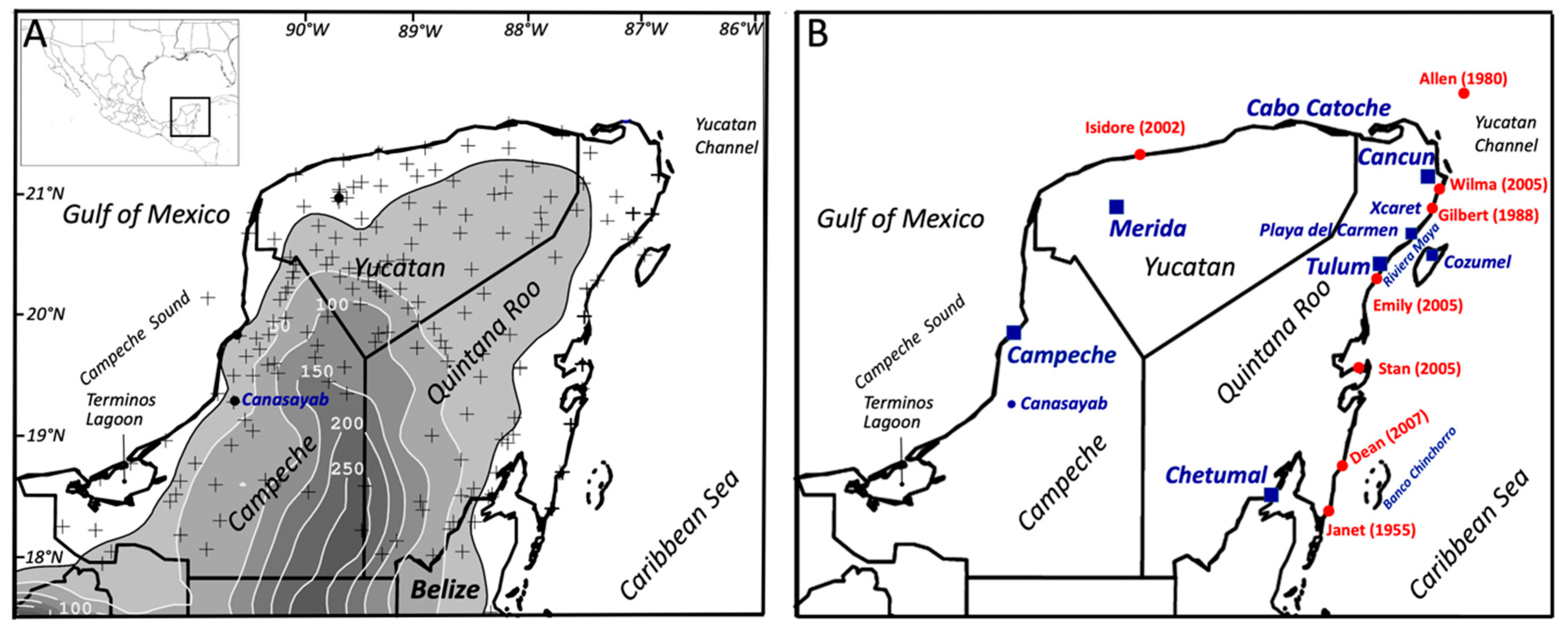
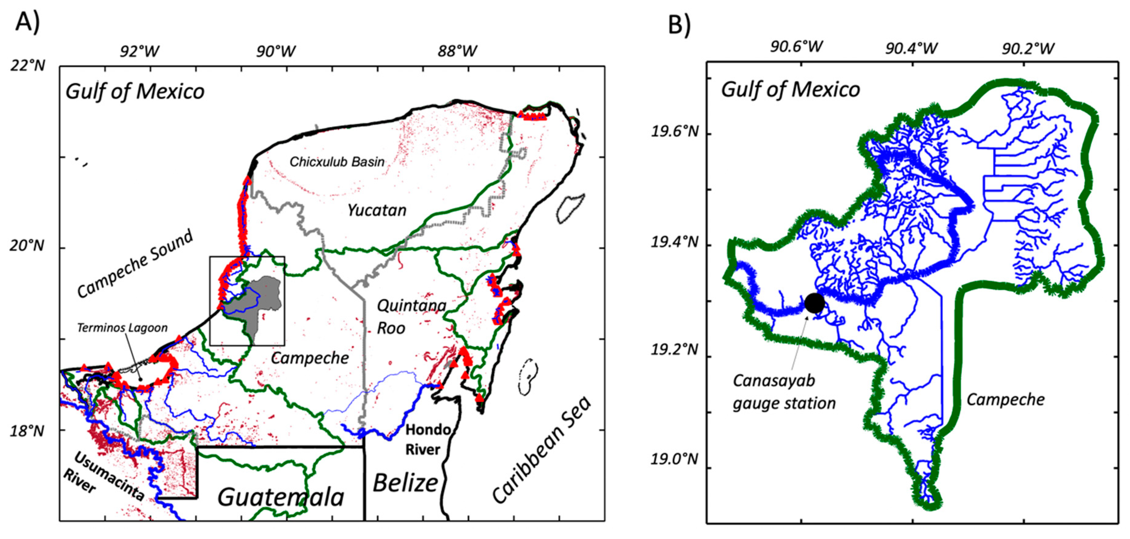
2.1. Area Description

The YP is located between latitudes 17° N and 22° N comprising the Mexican states of Quintana Roo, Yucatan, and Campeche, and northern Belize. The Mexican portion of the YP has 1941 km of shoreline representing 17% of the nation’s length, which is unevenly partitioned between the GOM (765 km) and the CS (1176 km); Belize’s shoreline in the YP extends only 386 km. In 2015, the population of the YP was ~4.9 million (Yucatan: 43%; Quintana Roo: 31%; Belize: 18%). The five largest cities in decreasing order of total population are Merida, Cancun, Campeche, Chetumal, and Playa del Carmen (5) (Figure 1B); coastal cities in Quintana Roo account for 45% of Mexico’s tourist revenue [52,53].

The average annual rainfall accumulation (1981–2010) was observed to be variable across the YP, with the highest values ranging from 1283–1333 mm (e.g., Merida, Cancun, Chetumal, Playa del Carmen, Canasayab) and lowest from 697–747 mm (e.g., Chicxulub, Dzilam, Celestun) [54,55]. The rainy season represents 70% of the annual total and occurs from May through October [56]. There are spatial differences in the precipitation distribution, with significant accumulations (800–1600 mm/year) in the southern and central peninsula while drier conditions (< 800 mm/year) are registered in the northern Yucatan state [57,58].

The regional geology consists of almost pure carbonate rocks and evaporites that define an unconfined flat lying karst landscape [37]. A distinct physiognomic structure is the Chicxulub basin, located in the northeast (Figure 2A). This basin is delimited by karstic sinkholes (“cenotes”) that route groundwater flow towards the central and northern YP [59]. Freshwater discharges occur mostly on the north coast supporting freshwater, brackish, and saline habitats, including productive wetlands and seagrasses in coastal and estuarine waters [40,60]. Relative ground elevations in the south range between sea level to ~300 m (Figure 1). The only significant topographic relief close to the coastline is in the southern region of the YP with a maximum elevation of 210 m. The northern coast of the peninsula is delineated by a series of lagoons where discharge is regulated by underground caves due to high rock permeability and gentle slopes [40,61]. Groundwater discharge along the Quintana Roo shoreline (e.g., Tulum; Figure 1), is distributed throughout a network of caves extending 8–12 km inland [62].

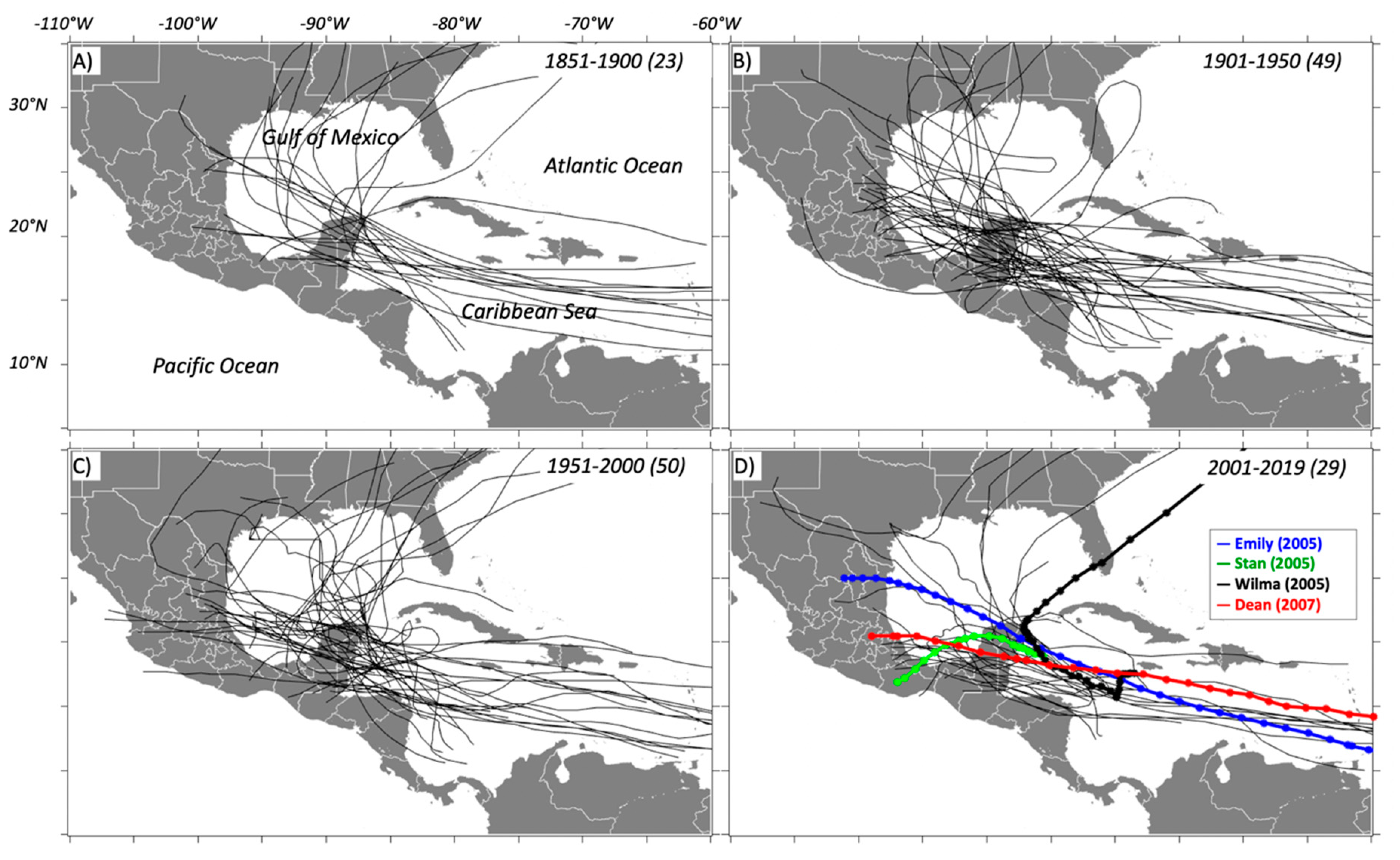
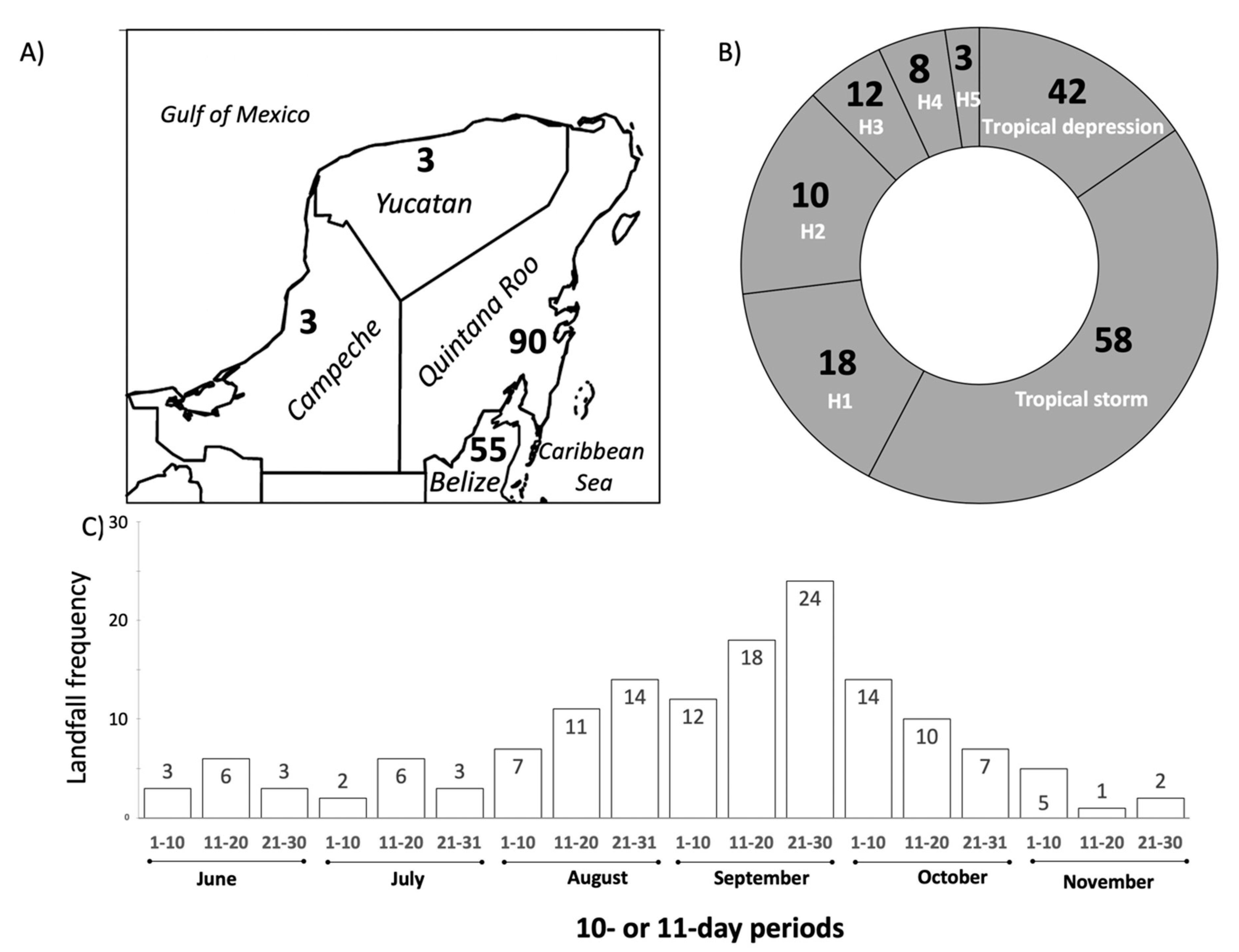
2.2. Tropical Cyclones

We used the TC historical data archive compiled by the United States National Hurricane Center (NHC). This dataset has reliable estimates of the center position and maximum sustained wind speed at six-hour intervals and at landfall [63]. Based on this wind speed during its entire lifecycle, each TC is classified in one of the following groups: tropical depression, tropical storm, or hurricane. Five hurricane categories (hereafter, HN; N = 1, 2, 3, 4, or 5) are assigned according to the Saffir–Simpson scale (e.g., [64,65]). We applied the above classification to establish the temporal and spatial characteristics of TCs that arrived in the YP. We examined 169 seasons (1851–2019) of activity in the north Atlantic basin, with 1894 TCs; most of the TCs had early stages over the central Atlantic and intensified while moving westward across the Caribbean Sea (Figure 3).

In addition to analyzing TCs’ physical features (e.g., trajectory, maximum wind, path) registered in each season, four storms were selected to further evaluate patterns in cloud cover, rainfall, vegetation changes, ocean Chl-a, and impacts on runoff (Figure 3D): Emily (H4; July 2005), Stan (tropical storm; October 2005), Wilma (H4; October 2005), and Dean (H5; August 2007). These TCs made landfall in Quintana Roo and were selected due to their variable intensity and considerable environmental impacts, including property damage, and population deaths throughout the YP (Supplemental Materials; Table S1).

2.3. Rain Gauge and Drainage Networks

To determine the spatial coverage and intensity patterns of selected precipitation events, we used records from a ground-based network of weather stations located throughout the study area and managed by the Mexican and Belizean meteorological services (Figure 1); daily records have been compiled from 248 stations in both countries. The datasets were partitioned by the timing of precipitation accumulations during five consecutive days, i.e., two days before landfall, the day of landfall, and then two days after landfall. A total of 166 stations located in the study region were selected per state and country (Figure 1A): 44 in Quintana Roo, 68 in Yucatan, 52 in Campeche, and 2 in Belize. As a climatological reference, records with significant rainfall from specific periods were compared to those from historical data with complete annual records (1981–2010).

Due to low topographic relief, no conspicuous surface drainage exists throughout the YP; runoff is from rainfall events recharging regional karst aquifers, which are the primary water source for human consumption and economic activities (e.g., livestock, agriculture) [37]. The hydrological connectivity between karst aquifers and seawater is closely coupled, and depending on interannual and seasonal variations, it can also promote saline intrusions reaching tens of kilometers inland [66,67]. The only streamflow gauge station in operation since 1956 is in the Champoton River basin (Figure 2B) north of the Usumacinta River system and its tributaries [68,69]. The river catchment area is 2583 km² while the gauge station drainage area is 2330 km². Long-term (1956–2014) and before, during, and after discharge values were estimated for each of the four storms included in the analysis.

2.4. Satellite Products

To determine the distribution of cloud cover and atmospheric humidity, as a proxy of precipitation, we used a dataset from the Geostationary Operational Environmental Satellite-12 (GOES-12) centered over the CS at 75° W [70]. The dataset includes imagery from the water vapor (6.5 μm) and infrared (13.3 μm) channels with a 4 × 8 km and 30-min spatial and temporal resolution, respectively. Infrared images are capable of measuring cloud-top temperature [71], thus providing an estimate of the cloud’s vertical development. Pixels colder than −60 °C generally delineate deep clouds in the TC core and within 444 km from the TC center (e.g., [71,72]). This temperature is at an elevation of ~13 km from July through October in the atmosphere over the CS [73,74]. To examine changes during the approach and landfall of selected TCs, we created a visualization tool (animation) available online (see Table S2) (https://met-bcs.cicese.mx/LSU). Specifically, this tool is a compilation of water vapor time-series to aid in the analysis of the TCs’ large-scale environmental impact and footprint [75]. A set of animations from this analysis is listed in the results section and the full list of web links is in Table S2 (Supplemental Materials).

We identified vegetation following TCs’ landfall using the Enhanced Vegetation Index (EVI) from the Moderate Resolution Imaging Spectroradiometer (MODIS) at a 250-m spatial resolution and the applied product MOD13Q1V from the on-line Google Earth Engine platform [76]. The EVI is derived from red (0.620–0.670 μm), near-infrared (0.841–0.876 μm), and blue (0.459–0.479 μm) reflectance bands; the EVI was averaged over time to detect vegetation change on a per-pixel basis [77]. This index minimizes canopy background variations, maintains sensitivity over dense vegetation, and includes an atmospheric correction along with a mask for water, clouds, and cloud shadows. The EVI has been used to assess TC impact on coastal vegetation (e.g., [78]) and is sensitive to structural variations in canopy structure. Here, we computed changes between two adjacent years for the periods with the same number of days before and after landfall to estimate either an increase (gain) or decrease (loss) of vegetation areas.

We used the surface satellite-based Chl-a values as a proxy to assess potential changes in coastal aquatic primary productivity (e.g., [79,80,81]) using daily satellite observations at 4 × 4-km spatial resolution (i.e., GlobColour; [82,83,84]) and level-4 processing provided by the European Space Agency [85]. These products are recommended for studies of small-scale and high-frequency phenomena in coastal areas [86]. The estimated Chl-a spatial differences were estimated before and after landfall along the YP coastal ocean bounded by the coordinates 18° N, 24° N, 85° W, and 93° W. These values were similar to Chl-a reported by other studies in the same coastal regions in the GOM [87,88,89]. We also evaluated the temporal changes of satellite-based Chl-a along a 850 km long transect at 25 m isobath from the Campeche sound and encompassing the states of Campeche, Yucatan, and partially, northern Quintana Roo coastlines. The Chl-a values along this transect are influenced by the potential interaction between the groundwater discharge and water column mixing [39,40] after TC landfall. The partial coverage of Quintana Roo’s coastline was selected to determine changes in Chl-a during TC impact at the western, northern, and eastern YP coastlines (Figure 1).

3. Results

3.1. Tropical Cyclones

The total number of TC landings on the YP, from 1851–2019, was 151 (Figure 4); 90 storms crossed Quintana Roo while 55 landed on Belize northern region. Landfall strength was variable, with most events arriving as tropical storms (58) followed by tropical depressions (42), and category-one (H1, 18) and category-two (H2, 10) hurricanes (Figure 4B). A lower number of events were identified as category-three (H3, 12), category-four (H4, 8), and category-five (H5, 3) hurricanes; these major hurricanes are characterized by destructive impact on vegetation structure and causing infrastructure damage in urban centers (Figure 4B). The highest landfall frequency (62%) occurred from mid-August through early October, with a general peak period from 21–30 September. The month with the most landings was September (54) followed by August (32) and October (31) (Figure 4C). The only category-5 hurricanes registered in the period were Janet (278 km/h at landfall; September 1955), Gilbert (259 km/h; September 1988), and Dean (278 km/h; August 2007). Additionally, two H5 hurricanes passed within 175 km of Cancun in August 1980 (Allen; 306 km/h) and September 2004 (Ivan; 259 km/h). Using wind speed as a TC-strength metric, Allen is considered the strongest in the whole Atlantic basin while crossing the Yucatan Channel [79] (Figure 1A). Three of the four storms selected for further regional environmental impact analysis occurred during the relatively active season of 2005 (Figure 3D). Dean (2007) is one of the 33 H5 hurricanes that developed in the North Atlantic since 1924 and the most powerful storm crossing the peninsula since 1988. Although Stan (2005) was a tropical storm providing heavy rainfall elsewhere in Mexico, accumulations were moderate across the YP [48].

Given their strength differences, Emily, Stan, Wilma, and Dean show distinct wind speeds at landfall (Figure 3D, Figure 5; Table S1). Wilma (213 km/h) and Emily (213 km/h) were H5 hurricanes over the Caribbean while Dean was the strongest (278 km/h) TC to cross Quintana Roo. Further, Wilma became an H5 hurricane 57.5 h before landfall but was weaker while landing on the YP coast (213 km/h). Due to the interaction with land, all TCs weakened during the next 6–12 h; although, after crossing the YP, Stan became stronger over the southern GOM and eventually crossed the state of Veracruz as an H1 hurricane (Figure 3D).

3.2. TCs Impacts: Emily, Stan, Wilma, and Dean

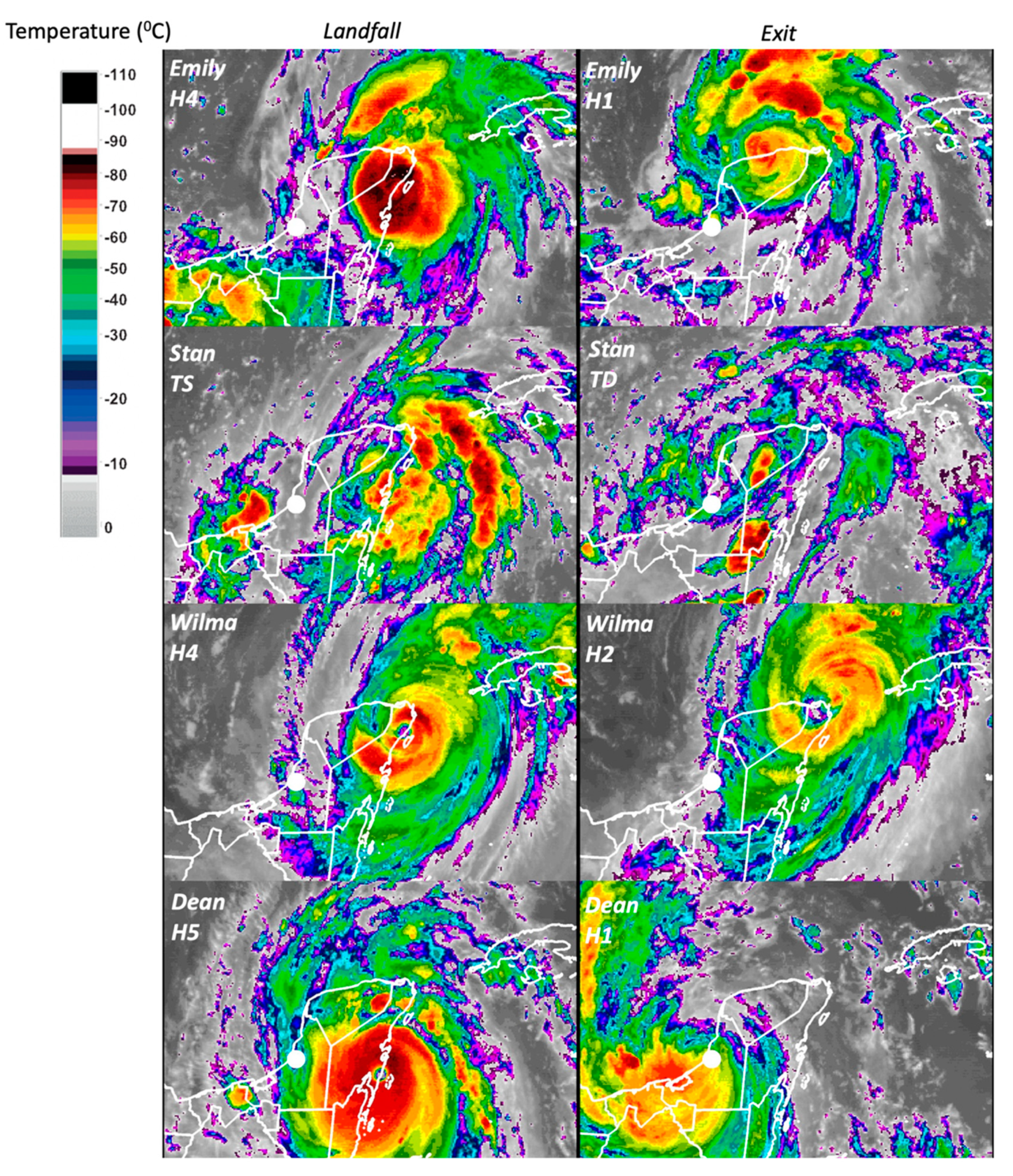
3.2.1. Cloud Cover

Cloud dispersion, coverage, and temperature over land were as expected related to TC motion and maximum speed at landfall (Table S2; Figure 5). During Emily’s landfall, near Xcaret (Figure 1B), areas with a cloud-top temperature <−60 °C covered portions of the northeastern YP, while a few isolated cells reached a temperature of −80 °C (altitude, 15 km) in Quintana Roo (Figure 6). An analysis of the landfall evolution revealed that on 18 July, 2005, this type of cell covered the northern region of the state and the northeastern Yucatan (https://met-bcs.cicese.mx/LSU/animation_emily.gif; Table S2). In contrast, Wilma had the largest area of influence (i.e., wind radii) with a circulation center remaining close to the coast (<150 km) for almost 48 h, 12 of them overland. Wilma’s and Dean’s impact was characterized by deep clouds over the YP and a large area off the Caribbean coast, which lasted for at least two days over Quintana Roo (21–22 October, https://metbcs.cicese.mx/LSU/animation_wilma.gif; Table S2). Furthermore, Dean’s intensity (21 August 2007) was the strongest at landfall (278 km h^-1; Table S1), covering a large cell with temperatures colder than −80 °C over the east across Campeche (Figure 6; Table S2) (https://metbcs.cicese.mx/LSU/animation_dean.gif).

Stan developed in early October 2005 and reached maximum wind speeds below 70 km/h and arrived as a tropical storm with slow motion (6 km/h) and a limited radius of influence. The cloud cover at landfall had a well-defined spiral band over the Yucatan Channel (Figure 1A; Figure 6) (https://met-bcs.cicese.mx/LSU/animation_stan.gif). Because of the interaction with the peninsular landmass, this TC weakened rapidly but emerged over the GOM as a tropical depression. Here, the TC circulation regained intensity and became an H1 hurricane moving over the southern GOM with maximum winds up to 130 km/h while approaching Veracruz, where it landed again. An extended imagery animation (not shown) provides evidence of deep cells with temperatures as cold as −100 °C, representing altitudes above 19 km.

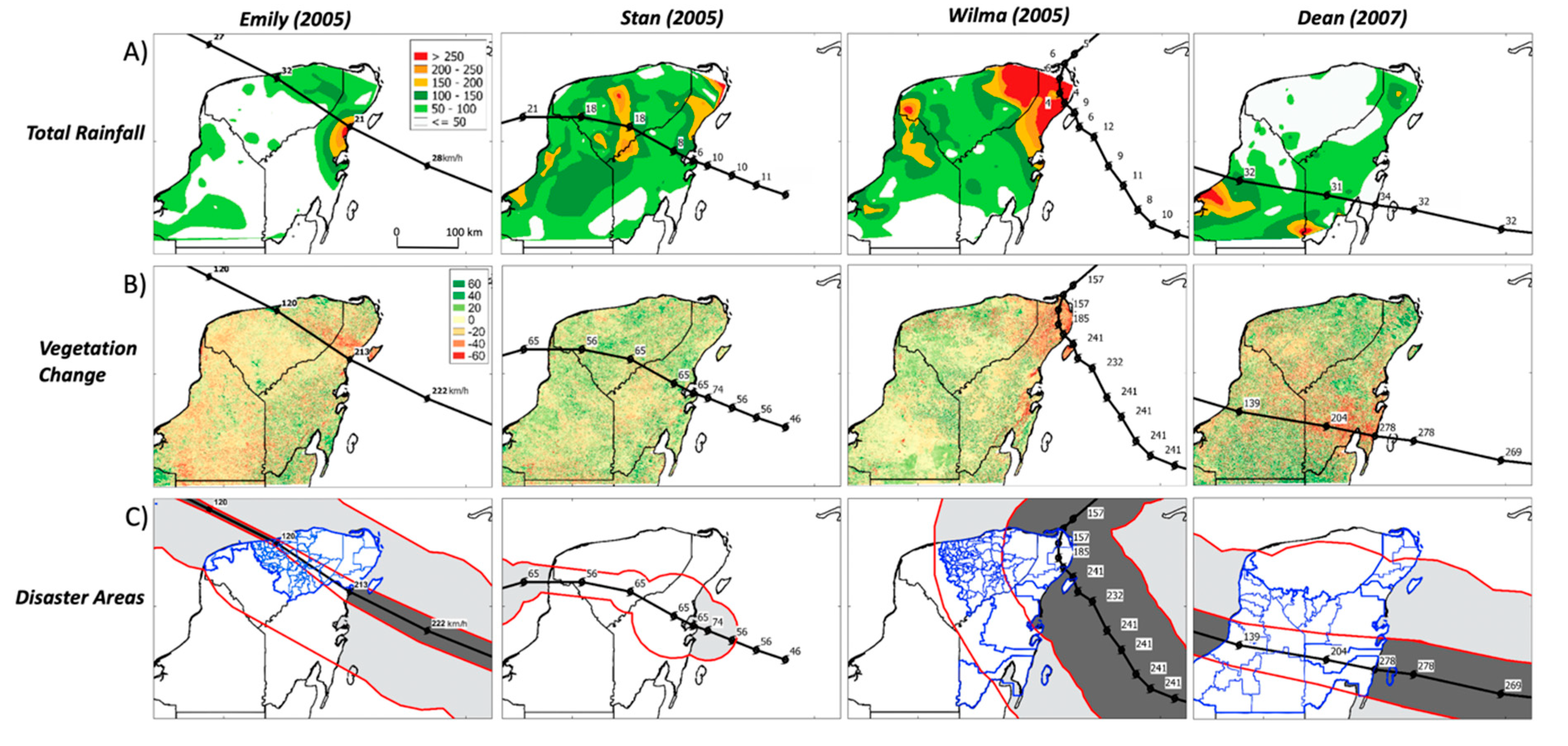
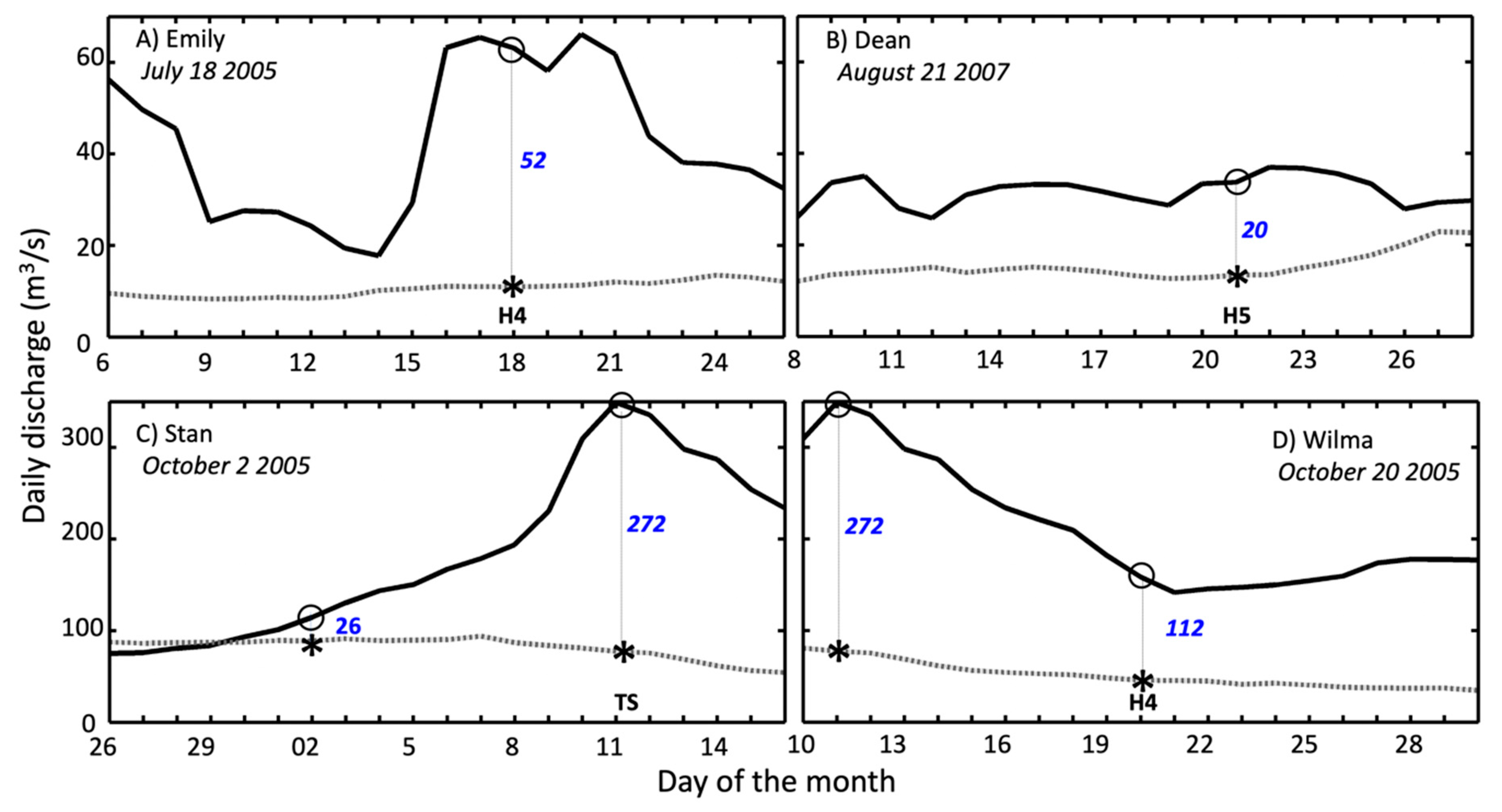
3.2.2. Rainfall and River Discharge

During Emily’s development over the YP, most rainfall accumulations (up to 300 mm) occurred near the landfall site in Tulum, Quintana Roo. Overall, totals ranged from 50–150 mm to the right (northeast) of Emily’s track (Figure 1, Figure 7A). In contrast, a more uniform rainfall distribution characterized Stan’s impact, with a 339-mm maximum in Cancun corresponding to a narrow area of winds above 63 km/h located to the northeast from the TC center (Figure 7A). Similarly, as Wilma approached the northeastern YP, the total accumulation was over 200 mm. Using Cancun observations from a 1981–2010 baseline, the record maximum registered was 770 mm on 20–21 October 2005, one day after Wilma’s landing. TC Dean arrived with the strongest winds, exceeding by 27 km/h the lower margin for an H5 hurricane, then moved quickly (31–34 km/h) while crossing the YP. This storm showed a different rainfall distribution, especially south of the storm track (Figure 7A).

The relationship between precipitation and river discharge was complex and regulated, not only by the TC strength and landing location but also by the cloud cover footprint. The YP lacks large river watersheds, except in the western region where the small Champoton River watershed (Campeche; Figure 2A) drains into the GOM (Figure 2B). A long-term mean daily discharge comparison (1956–2014) with river discharge registered after a TC landing showed not only an increase in discharge after landfall but some contrasts under different storm characteristics (Figure 8). For instance, although Emily crossed the YP farther away than Stan relative to the location of the Canasayab station (Figure 2B), the precipitation resulted in greater discharge a couple of days before landing (63 m³/s) and remained elevated (>50 m³/s for three days after its passage (18–21 June, 2005; Figure 8A); these values were much higher than the long-term mean (~11 m³/s).

Stan’s path through the YP and its emergence as a tropical depression north of the river catchment area strongly influenced streamflow discharge, which slowly increased and reached a peak (>300 m³/s) nine days after landfall (Figure 8C). Wilma, also an H4 hurricane, crossed the northeastern part of the YP, resulting in moderate discharge (140–180 m³/s, Figure 8D) after landfall. In contrast, Dean’s path south of the Champoton river showed little precipitation in its catchment area (Figure 7A), resulting in a steady discharge (20–40 m³/s) close to the long-term average following landfall (Figure 8B). Overall, the discharge was higher during Wilma (392%), Dean (229%), and Stan (150%) when compared with the long-term climatology. Although the GOES-12 imagery from Emily and Dean show similar dimensions at landfall (Figure 6), their precipitation patterns differed over the Champoton River watershed, leading to observed differences in river discharge.

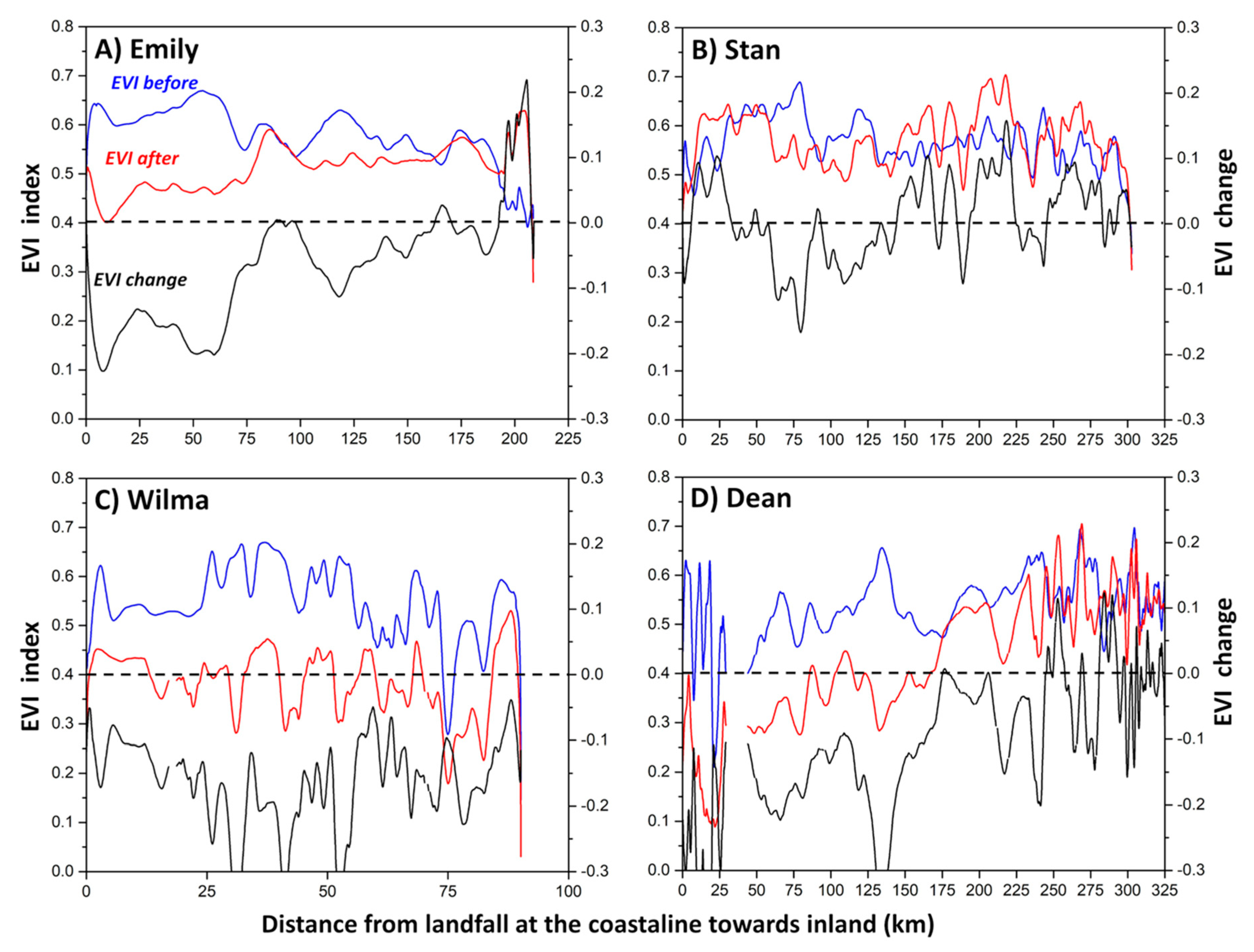
3.2.3. Enhanced Vegetation Index (EVI) Spatial Patterns

The EVI captured distinct changes in vegetation coverage after TC passage as shown in similar studies when assessing vegetation phenology or landscape-level vegetation differences [77,90]. A reduction of EVI was associated with TC strength; higher values (29%) were registered after Wilma and throughout the YP as result of Dean’s (20%) and Emily’s (7%) impacts (Figure 7B). These values contrast with a minor impact by Stan as shown by limited changes after landing. Vegetation changes due to Emily show a decline in a narrow area where TC winds were above 119 km/h for periods before (11–27 July 2004) and after landfall (12–28 July 2005). These changes depict a wide 63 km/h and 119 km/h radii, which are derived as the average from four directions, in the NHC chronology [63]. The most significant loss is just to the right (northeast) of Emily’s track, where speeds were nearly 119 km/h; the highest speed (180 km/h) occurred 24 km from the circulation center. In contrast, a limited decline in vegetation was observed to the left (southwest) of the storm core over western Yucatan, southern Quintana Roo, and Campeche.

Wilma’s maximum winds ranged from 222–241 km/h (Figure 5) and covered most of the YP northeastern tip. Areas with speeds above 119 km/h, and in the range of 63–119 km/h (tropical storm strength), comprised 14% and 48% of the YP total area, respectively. Wilma crossed Cozumel with approximately 215 km/h where a well-developed TC had an eye (Figure 6). In addition to the intense core, Wilma’s main damage to infrastructure was compounded by slow motion, with rates under 10 km/h, thus lasting longer over land (>24 h) before exiting the YP along the GOM and the Yucatan Channel. Most of the EVI changes occurred inside a wind-speed band above 119 km/h (Figure 7B); beyond this band (western Yucatan and in Campeche), only limited vegetation losses or gains were observed.

In the case of Dean, most of the vegetation losses were within 100 km from the Caribbean coast where mangrove forests were defoliated along the southern coast of Quintana Roo [91,92]. Wind speeds over the YP, southern Quintana Roo, and central Campeche were above 119 km/h across a radii ranging from 50 to 150 km. In contrast, Stan’s impact was minor and practically no areas with vegetation loss or gain were observed, even when speeds were in the range of 63–119 km/h while covering 24% of the YP. Comparatively, EVI profiles along the Emily (Figure 9A), Stan (Figure 9B), Wilma (Figure 9C), and Dean (Figure 9D) tracks revealed distinct differences. Yet, EVI averaged values were lower after landfall within the first 50–100 km, resulting in a net reduction in all four cases (Wilma: 29%, Dean: 20%, Emily: 7%, Stan: 2%; data not shown).

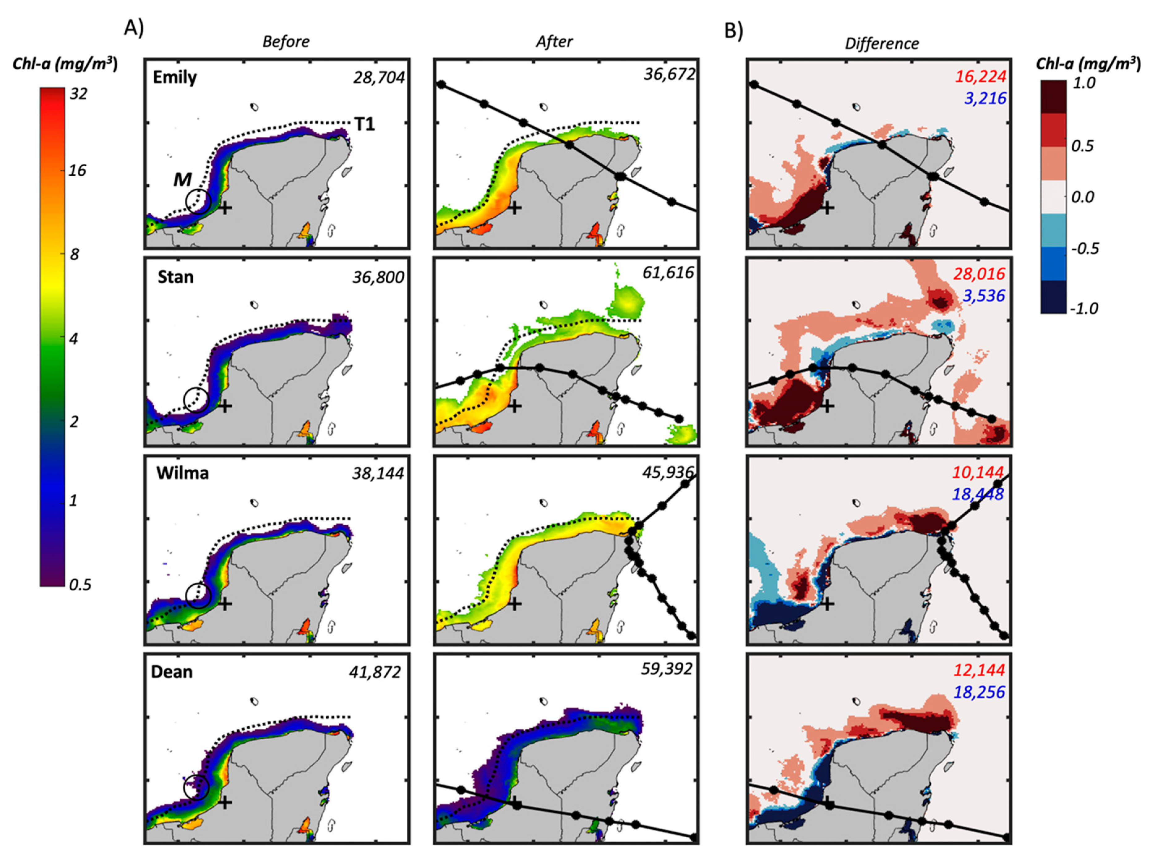
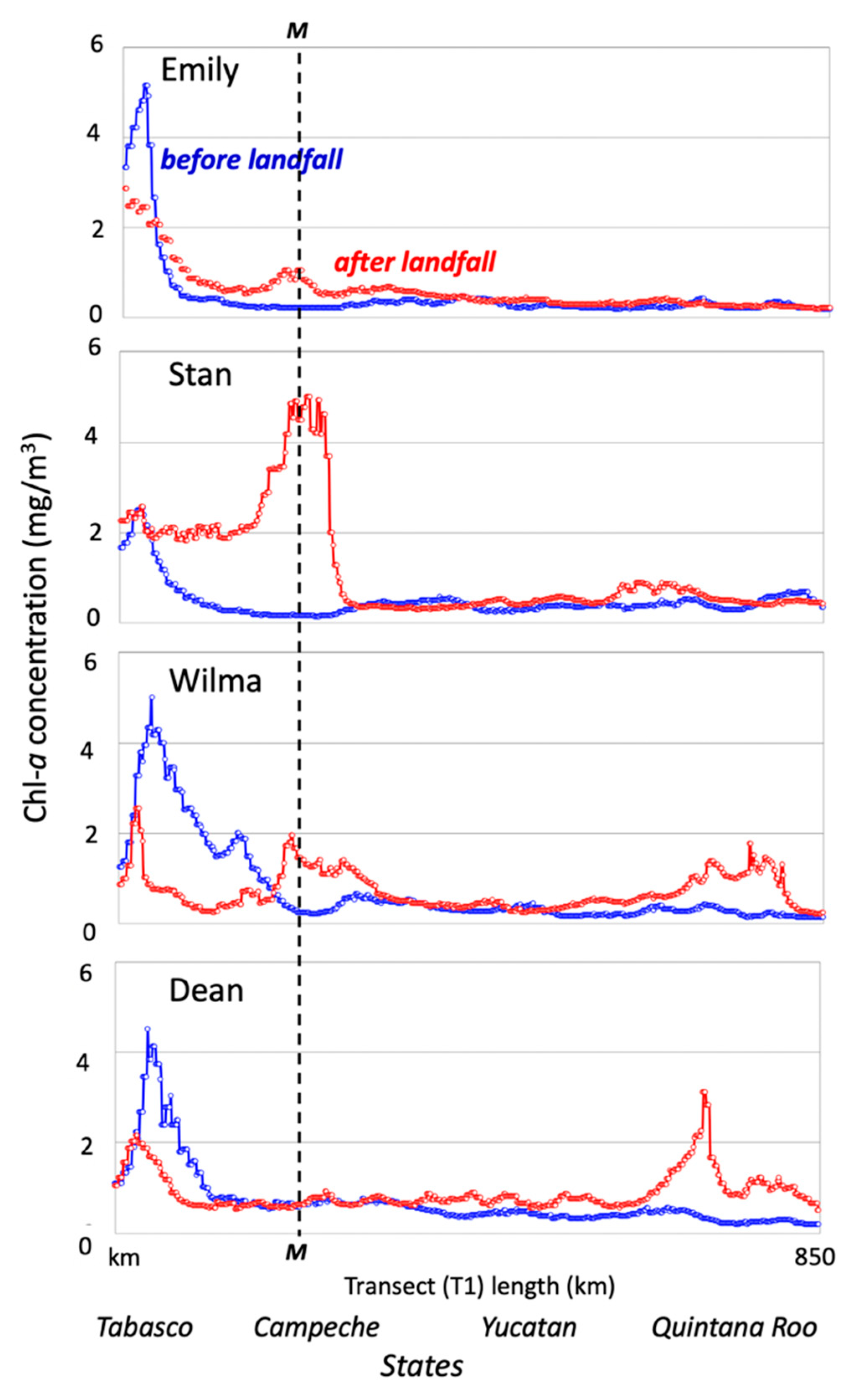
3.2.4. Coastal Chl-a Concentrations

Our analysis focused on seven days before and after TC landfall to determine spatial patterns associated with each TC trajectory, motion, and exit location (Figure 10 and Figure 11). Chl-a concentrations before landfall ranged between 0.5 and 2 mg/m³; these values decrease from the YP coastline towards the continental shelf, which is characterized by a smooth seafloor slope [93]. Except for the Chl-a distribution after Dean, concentrations increased above 10 mg/m³ in coastal areas after TC landfall, including Chetumal Bay, Cabo Catoche, Terminos Lagoon, and offshore in the central and northern Campeche coast (Figure 1B, Figure 10A).

Within the week following TC passage, there were spatial differences in the Chl-a distribution off the northern and western YP coastlines (Figure 10A). Areas represented by concentrations above 0.5 mg/m³increased in all cases from a baseline value before the storm impact of 42% after Dean’s passage followed by 28% in Emily and 20% in Wilma. A larger increase (67%) from the baseline value was associated with Stan (Figure 10A) along the Campeche coastal region. Most of the Chl-a enhancements were within 50 km from the YP, with a maximum extension up to 100 km northwest from Cabo Catoche (Figure 1B).

To evaluate the spatial changes of Chl-a, along the YP coastline, a transect was established along the 25-m isobath off the YP coastline (see Section 2.3; Figure 10A, dotted line) before and after each TC passage (Figure 11). While the Yucatan and Quintana Roo transect segments show a relative increase in Chl-a after the passage of Stan (138%), the increase was lower after Dean (26%) and Emily (24%). The maximum value along the transect after Stan’s passage was 5 mg/m³ and was located 120 km north of Terminos Lagoon (Figure 1), indicating the regional-scale impact of this TC over the southern (left) side of its center track. In contrast, Wilma crossed a limited portion of the YP, and the TC was more distant from the southern GOM; therefore, with some exceptions, there were no net changes in the Chl-a concentration along the transect (Figure 11).

In addition to the observed increase in Chl-a along the marine transect to evaluate the effect of TC trajectory and landing position in the GOM (Figure 11), we also observed an increase in concentrations higher than the average Chl-a (~0.5 mg/m³; [39]) in adjacent coastal and ocean water bounded within the 18° N, 24° N, 85° W, and 93° W coordinates (Figure 10B). Such upwelling in areas with average Chl-a values before the storm showed an increase in the total area depending on TC strength, track, and landing site: Stan (24,816 km²) > Dean (17,520 km²) > Emily (7968 km²) > Wilma (7792 km²). Overall, most of the Chl-a increase was observed near the shoreline, along northern Quintana Roo, Yucatan, and near the Terminos Lagoon (Figure 10B).

The passage of the Stan and Dean landings illustrate the degree of influence of surface water discharge on Chl-a values along the YP western coastline (Figure 10 and Figure 11). For example, the Champoton River discharge into the GOM on 11 October after Stan’s landing (Figure 8C) suggests a direct relationship between river discharge (up to 320 m³/s) and Chl-a up to 16 mg/m³. These conditions contrast with typical values (0.5–1 mg/m³; Figure 10A) found in oligotrophic waters and generally observed under normal (pre-storm) conditions [87,88,89]. In contrast, within one week after Dean’s passage across Campeche, river discharge was low (35-37 m³/s) with little change following landfall (Figure 8B). Under this river stage, Chl-a remained low along the coastline between the Champoton River and Terminos Lagoon (Figure 10A), where maximum Chl-a ranged from 1–3 mg/m³.

4. Discussion

4.1. Historical and Future Hurricane Frequency, Intensity, and Landfall

Our historical analysis highlights the Quintana Roo coastline as a TC hotspot where landing frequency is the highest followed by Yucatan and Campeche. A previous analysis of the periods 1851–2000 [94], 1951–2001 [95], 1970–2010 [31], and 1990–2011 [96] used similar NHC track and position records to analyze landfall patterns and observed this spatial trend separately, especially near Cancun [94]. Comparatively, the relative frequency in TC landings during the most recent period (2011 up to 2019) has not changed significantly, although long-term landings varied when the frequency analysis was performed on a decadal basis (Figure 4; Supplemental Materials, Figure S1).

We analyzed 1894 TC tracks from 1851 to 2019 across the Atlantic basin, where only 151 (~ 8% of the total) reached the YP. The most active landfall season was in 1931 when six TCs made landfall in the peninsula while four TCs landed in the seasons of 1933, 1942, 1971, 2005, and 2010 (Figure S1); in 2005, two events occurred in both July and October, respectively. After landfall, most TCs tend to move into the GOM, either weakening over central Mexico or the southern United States. Wilma was an extraordinary major hurricane, concerning the Atlantic basin activity, and comparable to other strong landfall events in other basins around the world [96,97]. Wilma also leads a group of TCs with maximum intensity over the ocean as determined by satellite data [98]. If the period of record is narrowed to 1995–2005, Wilma is one of eight major hurricanes reaching maximum intensity over the western Caribbean, south of the Yucatan Channel, and east of Quintana Roo ([99]; Figure 3)] (Table S1).

Although it is hypothesized that storm frequency will increase overall in the Atlantic basin as a result of climate change [100,101,102], it is not clear how the interaction between climate variability and change will specifically affect regional storm landings’ location, frequency, and strength across the Caribbean basin and the YP. These projections are needed to determine the regional, annual, and decadal impact on the hydrological cycle, particularly in the case of precipitation (e.g., [103]). This is the main source to recharge aquifers, supporting drinking water demands and rain-fed agriculture throughout the YP [104,105]. These aquifers are widely distributed due to the YP karstic geology and influenced by different regional climates [54,57].

4.2. Precipitation and River Discharge Spatiotemporal Patterns Induced by TC Impacts

Our analysis shows the dynamic relationship between TC strength and landing location in regulating precipitation throughout the YP’s diverse regional climates [55,104]. Wilma (H4) was a “rainmaker” causing extraordinary rainfall in the northeastern YP associated to the largest radii of moderate (≥63 km/h) and strong (≥119 km/h) wind speeds (Figure 7); its slow motion (≤12 km/h) provided enough exposure and caused not only more vegetation loss and changes in the Chl-a distribution (see section below) but also heavy rainfall when compared to TC precipitable water, a metric of moisture content in the atmosphere [106,107]. Wilma’s precipitable water ranged from 50-60 mm, which is larger than the average value considered to be a boundary favorable to TC rainfall production. While Wilma’s rainfall highly correlated with high rain-gauge observations (400–500 mm in five days), maximum accumulations (300–500 mm) associated with Stan were also observed elsewhere over the Isthmus of Tehuantepec, Guatemala, and portions of the EPAC and GOM. In contrast, a drier environment was present during the passage of Emily (35–45 mm in precipitable water) and Dean’s (38–60 mm), with limited rainfall accumulations (50–150 mm) throughout the YP.

A recent spatiotemporal assessment shows three distinctive precipitation clusters using data from 1980-2011, highlighting the regulatory effect of climatic variability across the YP [104]. These observed clusters show regions with the lowest precipitation values in the northern YP and the highest values in the southwest and southeast [55,104]. Preliminary climate modeling results at the regional scale indicate that the driest of the semi-arid climates will extend along the northern YP where a warmer climate might occur along the western and central sections of the peninsula [102]. How these local climates and associated precipitation will change as temperature increases at the regional scale by 2050 is unknown, especially as climate is modified by pulsing TCs. Further, the explicit simulation of TCs in climate models is still limited due to validation and the implementation and development of robust downscaling techniques [100,101,108]. The most recent downscaling estimates indicate that the YP will experience more extreme climatic events, including increasing TC frequency and intensification [102].

Because of the YP karstic geomorphic origin and low topography, not all the precipitation is diverted into watersheds and most infiltrate into extensive aquifers [38,109]. The large Champoton River catchment area is the only well-defined watershed in the YP where the Canasayab gauge station measures river discharge. We used discharge data from the station to evaluate the interaction among the TC landing area, trajectory, total rainfall, and cloud cover in influencing surface runoff timing and magnitude. This runoff, along with submarine discharge, has a significant impact on coastal primary productivity due to potential nutrient export (e.g., nitrogen; [39]) as observed overall in the YP and other coastal systems (e.g., [42]).

Despite the differences in strength and trajectories, Stan and Wilma produced almost the same net discharge (272 m³/s) (Figure 8). This discharge rate was almost three times higher than the value estimated from the 1956–2014 average baseline. In the case of Stan, the maximum discharge occurred 9 days after landing while the maximum for Wilma was also recorded within 9 days but before the storm’s landing. This delay underscores the asynchrony between the landing time and the net water discharge controlled by the storm path and acceleration while crossing the YP. Comparatively, the maximum net river discharge caused by Emily (52 m³/s) and Dean (23 m³/s) was lower than those from the other storms at the landing time. These major differences in net water discharge closely reflect, independently of the TC trajectory, the complex interaction between cloud coverage, precipitation, and storm motion. Determining the coupling between both the land and TC structure and biophysical properties is paramount to quantitatively evaluate ecosystem responses in the long term, especially when incorporating these data into climate models.

4.3. TC Impacts on Terrestrial Vegetation and Chl-a Concentration in Coastal Waters

Although we do not provide direct measurements of vegetation biomass or productivity rates, the use of EVI relative change (Figure 9) and Chl-a (Figure 10 and Figure 11) are good proxies to establish quantitative ecological impacts by TCs at the landscape/seascape level. These estimates show the utility of EVI as a good indicator of vegetation changes and damage when assessing ecological impacts directly related to TC strength [13]. Previous (EVI) vegetation studies across the YP have also been able to differentiate other functional ecosystem attributes, such as forest phenology [60], forest degradation due to both deforestation [110] and TC impacts [31,111], vegetation health regulated by land use/change and precipitation patterns [112], and gross primary productivity fluctuations related to landscape-level seasonal evapotranspiration flux [113].

In all four storms included in our analysis, the reduction in EVI was negatively associated to the wide bands of hurricane-wind force associated with Dean’s impact (i.e., 278 km/h) followed by Wilma and Emily (213 km/h). EVI changes along the inland path illustrated the trend and degree of the negative impact. Even when Wilma crossed a relatively small track of land (90 km; Figure 9C), in comparison to the other storms, EVI change values were negative throughout most of its track. A similar pattern was also observed in the case of Dean, where net EVI changes were also consistent along its 335-km track. In contrast, as result of the narrow and weaker speeds, EVI changes were lower along Emily’s 215-km continental path, with most impacts observed within the first 100 km, while Stan’s path showed negative EVI values in only a small segment representing <30% of its 300-km inland path.

Given the different levels of TC impact indicated by the negative EVI, all vegetation, including agricultural areas located in the northern region, were cumulatively impacted by the 2005 storms (Emily, July; Stan and Wilma, October). The impact was not only related to plant mortality but also to water availability in the long term. Indeed, water resources in the YP are limited as indicated by interannual variation in drought frequency and duration [55,57,104,114,115]. Since interannual precipitation is driven by TC frequency [104], water availability in the YP is variable where either a surplus or deficit can represent a legacy that influence vegetation resilience. This hydrological status is functionally critical since most of the YP is dominated by deciduous forest [116] that depends on TC-induced precipitation for reproduction and growth [110]. Previous studies indicate that years identified as the driest in a long-term series (2000-2014) show a relationship with the deficit of TCs affecting the YP. This dependence is apparently controlled by the presence of “El Niño” episodes, while the wettest years might be related to a greater number of TCs due to the presence of “La Niña” periods [113]. However, the ENSO attribution as a climate variability driver controlling TC frequency in the YP needs to be weighted and further evaluated, especially in the context of climate change as the TC internal structure (i.e., “rain-maker”) is significantly influenced by increasing global warming [25].

Another link between TC physical attributes (e.g., strength, trajectory) and ecosystem function is the spatiotemporal variation of Chl-a along the YP coastal zone. Our comparative analysis shows a significant increase in Chl-a after TC passage along with localized impacts depending on the storm exit point along the coast; this increase has been observed in other regions of the CS, west of the YP (e.g., Banco Chinchorro, Figure 1B; [117]). By considering a concentration of 0.5 mg/m³ as an average baseline, we identified enhanced areas (>15,000 km², Figure 10B) with concentrations >0.5 mg/m³ after the passage of Stan and Emily. Under normal conditions, average Chl-a offshore of the Campeche Sound have been reported to be in the range from 0.6 to 2.5 mg/m³ in areas adjacent to the coastline [118]. The highest Chl-a estimated for Stan in the northeastern (7-8 mg/m³; Figure 10A) and east (>8 mg/m³) regions of the YP might be related to the weaker wind speeds (<74 km/h; Figure 5) but longer residence time over the YP in comparison to the other TCs. We hypothesize that such an increase in Chl-a, up to 4x the average annual value, is caused by the interaction between hydrostatic pressure and storm-induced precipitation, promoting water column mixing offshore, submarine discharge, and excess surface water run-off within hours after TC impact. This increase in Chl-a has been characterized as “anomalies” without a direct attribution to TCs (e.g., [87]). Because the YP is basically a large karst aquifer (~165,000 km²) with complex groundwater hydraulic conductivity [37], submarine discharge is a key lateral water flux that hydrologically connects the YP with adjacent coastal waters, particularly during the wet season [38,119]. It is estimated that submarine groundwater discharge in the YP ranges from 36–95 m³ m^-1 d^-1 and contains about 75% of terrestrial groundwater [120]. The transport of nutrients via this submarine discharge has been measured at some locations along the YP Caribbean coast [62,121], although further work is needed to evaluate loading rates in the northern and western coasts [39,66,122].

Increasing human activities (e.g., agriculture, industry/urban development, tourism) in the YP during the last 20 years has exacerbated groundwater eutrophication and is presently a problem affecting water quality and human health as indicated by the presence of toxic algae blooms [40], microalgae extension [123], pharmaceutical products [123], and high nitrate concentrations from fertilizers [41,121,123,124,125]. Thus, the increasing eutrophication of the YP’s aquifers and corresponding submarine water discharge currently compares to other large river-dominated watersheds in the GOM. In these coastal zones, peak discharge drives both high Chl-a and water column productivity (e.g., Apalachicola River, [126,127]; Mississippi River, [128]; Galveston Bay, [129,130]; Grijalva-Usumacinta River; [131,132]), similar to the pulsing discharge induced after storm passage.

When building a landscape-level water balances for the YP, surface water run-off is generally ignored [113]. Yet, run-off caused by TCs becomes a significant pulsing of freshwater and nutrients inputs into the coastal zone as indicated by the variable discharge from the Champoton River. This export was indirectly gauged by analyzing changes in Chl-a along the transect depicted in Figure 10, which extends off the coast along the periphery of the YP encompassing the coastline of Campeche, Yucatan, and partially, northern Quintana Roo. Chl-a along this transect shows a sharp increase after Stan (5 mg/m³; Figure 11) and Dean (~3 mg/m³; Figure 11) in the southeastern region of Campeche, where surface run-off is more common due changes in elevation and the presence of large watersheds (e.g., Grijalva-Usumacinta; [132]) and associated estuarine end members. For instance, Terminos lagoon (Figure 1B), the largest coastal Lagoon in Mexico (2500 km²; [133]) and part of the Grijalva-Usumacinta deltaic system [134], exports inorganic nutrients and organic matter to the adjacent Campeche Sound during peak river discharge and strong tidal exchange [135]. This export is noticeable in large plumes of freshwater extending into the Sound with moderate Chl-a (<4 mg/m³) after Emily, Stan, Wilma, and Dean passage (Figure 1 and Figure 10A). In contrast, the absence of high Chl-a peaks (>0.5 mg/m³) along the transect beyond the state of Campeche in the case of Dean (Figure 11) underscores the complex interaction between the storm trajectory, rainfall patterns before and after landing, and the YP geohydrology. This interaction among those factors is illustrated by the increase in Chl-a >0.5 mg/m³ on the northeastern tip of the YP (i.e., Cabo Catoche; Figure 10B) following the passage of both Wilma (~10 mg/m³) and Dean (~4 mg/m³). Indeed, this coastal region is identified as both a major groundwater recharge area [37] and a seasonal upwelling region where phytoplankton blooms (mean Chl-a 1.45 mg/m³; [79,80,81]) are fueled by Ekman-layer transport and slope water intrusion from the Yucatan channel.

How this increase in Chl-a caused by pulsing TCs will impact secondary production (e.g., fisheries) in the long term along the YP coastal regions is unknown [136]. In addition to an increase in Chl-a induced by both submarine discharge and upwelling in the Yucatan continental shelf [79,81], surface run-off can also modify phytoplankton community structure and diversity [129]. Previous studies in phytoplankton community variations along the northern YP coastline show that subterranean water discharge interacting with coastal waters’ water quality and salinity play a key role in relative differences in dominance, for example, of thick-valve pennate diatoms and dinoflagellates among sites [122]. This difference in phytoplankton groups and taxonomy significantly influences upper trophic levels in the pelagic food webs (i.e., trophic cascade; [43,137]). For instance, despite the overall oligotrophic conditions of the YP coastal waters, especially in the Caribbean region, biodiversity [138] and secondary production is high, characterized by extensive coral reefs [139,140,141,142] and charismatic filter-feeding, e.g., whale sharks and rays [47,143], and sea turtles [144]. Further, key ecosystems services, such as artisanal and industrial fisheries, represent a critical economic source providing a combined value (i.e., Campeche, Yucatan, Quintana Roo) ranging from US $130-180 million in the period from 2006-2014 [145,146]; these fisheries include shrimp [147], red grouper [45,148], sea cucumber [46], octopus [149,150], and lobster [151,152]. If TC frequency and strength increases in the next decades as forecasted by climate models and recent global warming trends [25,102], then major changes in the food web structure/dynamics and associated ecosystem services should be expected. Further systematic work is needed to directly measure nutrient loading rates controlled by groundwater discharge in the long term along the YP coastline, especially before and after storm passage (e.g., [9,21]). Overall, there is still a lack of data and information needed to determine if extreme climatic events, such as wetter than normal years caused by TC or droughts, determine whether a specific coastal region will act as a recharge or discharge zone [113,121], thus influencing coastal trophodynamics in the long term [43].

4.4. Regional Socio-Ecological and Economic Impacts under Climate Change

In contrast to some of the positive TC impact on ecosystems’ productivity (Chl-a, EVI) and water availability (precipitation, run-off, groundwater recharge), a negative impact on population centers (deaths) and losses (agriculture, forest areas) also represent the common metric in how these extreme climatic events are assessed not only in Mexico but globally [153,154,155,156,157]. Because the YP is the third TC landing “hot spot” in Mexico, after the Baja California Peninsula and the state of Sinaloa in the EPAC coast [31,95,158], the socioeconomic impact is high. Using the Mexican government assessment criteria to allocate financial support after a storm impact, we determined the differences in population density impacted by Emily, Stan, Wilma, and Dean (Supplemental Materials, Table S3; Figure 7C) [159]. We identified a close relationship between the severity of vegetation losses (EVI index; Figure 7B) and total population affected based on the spatial distribution of wind fields and strength (Table S3). For example, Wilma affected more people (one million) in the YP than Dean (140,000) while Stan caused more property damage (US $2.5 billion) outside the YP region due to extraordinary precipitation and associated floods in Central America and southeastern Mexico [48].

When comparing the number of disaster areas and the total population impacted by the 10 top TCs from 1988–2016, Wilma is first (80 areas; one million affected) followed by Emily (58; none) and Isidore (93; 500,030), which made landfall as an H3 hurricane in 2002 (Table S1). This regional difference in affected population is partially explained by the variable number of administrative areas per state in the YP; while there were 106 areas in Yucatan, only 11 were identified in both Quintana Roo and Campeche (Figure 7), underscoring how differences in TC trajectory and humidity content, and not necessarily strength (i.e., wind speed), can produce different economic impacts. This spatially explicit property damage and deaths per region can also be highlighted using municipalities to delineate a regional impact; a municipality is the second-level administrative division of each state, which receives financial support from Mexico’s federal government in response to a natural disaster. Figure 7C shows that most of the disaster areas are within the boundaries of moderate (63–119 km/h) or intense (>119 km/h) speeds along with the vulnerability of Quintana Roo, where the frequency of TC is the highest in comparison to Campeche and Yucatan. This spatial comparison also shows how inland and coastal areas in the YP can be impacted within one single year, as was the case in the season of 2005.

Despite the hazardous status of the Quintana Roo’s coastline due to its geographical position as a TC “hot spot”, the state’s economic activity has dramatically increased during the last 30 years becoming one the fastest growing urban and tourism regions in Mexico (e.g., [160,161,162]). For example, the change in population density change from 1970 (1.8 people/km²) to 2015 (29.8) represents a 1555% increase (Supplemental Materials, Table S4). Further, it is estimated that the tourism industry in this coastal area contributes annually with more than 8 billion dollars to the Mexican economy [52]. However, the increasing threat to human well-being and infrastructure by TCs shows a non-linear trend, where, for instance, the cost of inaction in developing mitigation and adaptation strategies to these threats can range from US $1.4 to $2.3 billion under 2–3-m sea level rise (SLR) scenarios [52].

This interaction between TCs impacts and SLR is now a major vulnerability issue not only to coastal cities in Quintana Roo (e.g., Cancun, Playa del Carmen, Cozumel; [52]) but also to cities in Campeche (e.g., Ciudad del Carmen, Campeche City) and Yucatan (e.g., Celestun, Progreso), in terms of economic development and sustainability [163,164]. For instance, Wilma had a major economic impact by affecting the local population and 62,000 tourists visiting Cancun and the Riviera Maya (Figure 1B; Figure 7). The estimated economic impact for Mexico was approximately US $5 billion [159], including damage to hotel infrastructure in Cancun. Comparatively, this economic damage is higher than the combined damage caused by Stan (US $2.5 billion), Emily (US $400 million), and Dean (US $600 million) [159]. Thus, disaster risk along Quintana Roo’s coastline is compounded by the multiple effect of complex interactions among vulnerability, exposure, and hazard [4,153,165]. Yet, there is a lack of studies assessing future economic scenarios and planning that should consider those functional elements of risk, including the recognition of threats posed by climate change and the need to identify and implement adaptation strategies throughout the YP [4,52,161]. Overall, building resilience in current and future adaptation policies is urgently needed. This is the case not only in the YP but in the rest of the Mexican states along the GOM and EPAC coasts, due to the unique “double jeopardy” driven by TC landfall hot spots that increasingly and independently impact the extensive nation’s coastline.

5. Summary and Conclusions

Mexico is exposed to TC landings from the eastern Pacific and north Atlantic Ocean basins. Given the difference in landing frequency, we analyzed landfall events across the Yucatan Peninsula (YP) located between the Gulf of Mexico (GOM) and the Caribbean Sea (CS); this region is characterized by karstic geology where precipitation mostly infiltrates into the aquifers due to the lack of rivers. To identify vulnerable “hotspots” across the YP, we used a historical archive (1851–2019) of Atlantic TCs to evaluate the frequency, trajectory, and intensity of 151 landfall events. Most of the landings (60%) occurred along the YP eastern coast (state of Quintana Roo) between the months of August and September. Based on remote sensing datasets from operational satellites, we analyzed three major hurricanes (Emily and Wilma, 2005; Dean, 2007) and one tropical storm (Stan, 2005) to estimate impacts on vegetation (EVI) and coastal phytoplankton (Chl-a). Daily discharge records from a regional network were used to estimate rainfall accumulations. Similarly, the Canasayab gauge station located in the western peninsula (Campeche) was used to estimate the Champoton River discharge associated to TC passage. Interestingly, the highest discharge rate was observed during a period of 5–15 days after the passage of Stan (2005), in contrast to a limited discharge rate caused by the most intense hurricane (i.e., Dean, 2007).

Despite a short path through the landmass (Quintana Roo), hurricane Wilma caused more vegetation losses than any other TC; this damage occurred under strong winds, slow motion, and heavy precipitation. Unusually intense or persistent rainfall from TCs resulted in streamflow significantly exceeding the long-term (1956–2014) climatological mean. Most TCs caused a significant increase in Chl-a; we hypothesize that such an increase, up to 4 times the annual average, was due to the interaction between hydrostatic pressure and storm-induced precipitation promoting water column mixing offshore, submarine discharge, and excess surface water run-off within hours after TC impact. When comparing the number of disaster areas associated to the total population impacted by the 10 top TCs, from 1988–2016, Wilma is at the forefront with more disaster areas than Emily and Dean. Although disaster areas after Stan were not recorded in the YP proper after passage, this storm caused heavy rainfall and population impact in southeastern Mexico. Disaster risk along the YP coast underscores the negative economic impacts and positive ecological benefits at the regional scale.

References

1. Anthes, R.A. Tropical Cyclones, Their Evolution, Structure and Effects; American Metereological Society: Boston, MA, USA, 1982. [Google Scholar] [CrossRef]
2. Kousky, C. Disasters as Learning Experiences or Disasters as Policy Opportunities? Examining Flood Insurance Purchases after Hurricanes. Risk Anal. 2017, 37, 517–530. [Google Scholar] [CrossRef]
3. Auffhammer, M. Quantifying Economic Damages from Climate Change. J. Econ. Perspect. 2018, 32, 33–52. [Google Scholar] [CrossRef] [Green Version]
4. Diaz, D.; Moore, F. Quantifying the economic risks of climate change. Nat. Clim. Chang. 2017, 7, 774–782. [Google Scholar] [CrossRef]
5. Paerl, H.W.; Bales, J.D.; Ausley, L.W.; Buzzelli, C.P.; Crowder, L.B.; Eby, L.A.; Fear, J.M.; Go, M.; Peierls, B.L.; Richardson, T.L.; et al. Ecosystem impacts of three sequential hurricanes (Dennis, Floyd, and Irene) on the United States’ largest lagoonal estuary, Pamlico Sound, NC. Proc. Natl. Acad. Sci. USA 2001, 98, 5655–5660. [Google Scholar] [CrossRef] [Green Version]
6. Paerl, H.W.; Valdes, L.M.; Peierls, B.L.; Adolf, J.E.; Harding, L.W. Anthropogenic and climatic influences on the eutrophication of large estuarine ecosystems. Limnol. Oceanogr. 2006, 51, 448–462. [Google Scholar] [CrossRef] [Green Version]
7. Greening, H.; Doering, P.; Corbett, C. Hurricane impacts on coastal ecosystems. Estuaries Coasts 2006, 29, 877–879. [Google Scholar] [CrossRef]
8. Tanner, E.V.J.; Kapos, V.; Healey, J.R. Hurricane Effects on Forest Ecosystems in the Caribbean. Biotropica 1991, 23, 513–521. [Google Scholar] [CrossRef]
9. Lugo, A.E. Visible and invisible effects of hurricanes on forest ecosystems: An international review. Austral Ecol. 2008, 33, 368–398. [Google Scholar] [CrossRef]
10. Day, J.W.; Boesch, D.F.; Clairain, E.J.; Kemp, G.P.; Laska, S.B.; Mitsch, W.J.; Orth, K.; Mashriqui, H.; Reed, D.J.; Shabman, L.; et al. Restoration of the Mississippi Delta: Lessons from Hurricanes Katrina and Rita. Science 2007, 315, 1679–1684. [Google Scholar] [CrossRef] [PubMed] [Green Version]
11. Nyman, J.A.; Delaune, R.D.; Pezeshki, S.R.; Patrick, W.H. Organic-Matter Fluxes and Marsh Stability in a Rapidly Submerging Estuarine Marsh. Estuaries 1995, 18, 207–218. [Google Scholar] [CrossRef]
12. Smith, J.E.; Bentley, S.J.; Snedden, G.A.; White, C. What Role do Hurricanes Play in Sediment Delivery to Subsiding River Deltas? Sci. Rep. 2015, 5, 1–8. [Google Scholar] [CrossRef] [PubMed]
13. Wang, W.T.; Qu, J.J.; Hao, X.J.; Liu, Y.Q.; Stanturf, J.A. Post-hurricane forest damage assessment using satellite remote sensing. Agric. For. Meteorol. 2010, 150, 122–132. [Google Scholar] [CrossRef]
14. Potter, C. Global assessment of damage to coastal ecosystem vegetation from tropical storms. Remote Sens. Lett. 2014, 5, 315–322. [Google Scholar] [CrossRef] [Green Version]
15. Tapia-Palacios, M.A.; Garcia-Suarez, O.; Sotomayor-Bonilla, J.; Silva-Magana, M.A.; Perez-Ortiz, G.; Espinosa-Garcia, A.C.; Ortega-Huerta, M.A.; Diaz-Avalos, C.; Suzan, G.; Mazari-Hiriart, M. Abiotic and biotic changes at the basin scale in a tropical dry forest landscape after Hurricanes Jova and Patricia in Jalisco, Mexico. For. Ecol. Manag. 2018, 426, 18–26. [Google Scholar] [CrossRef]
16. Castaneda-Moya, E.; Rivera-Monroy, V.H.; Chambers, R.M.; Zhao, X.C.; Lamb-Wotton, L.; Gorsky, A.; Gaiser, E.E.; Troxler, T.G.; Kominoski, J.S.; Hiatt, M. Hurricanes fertilize mangrove forests in the Gulf of Mexico (Florida Everglades, USA). Proc. Natl. Acad. Sci. USA 2020, 117, 4831–4841. [Google Scholar] [CrossRef] [PubMed]
17. Knutson, T.R.; McBride, J.L.; Chan, J.; Emanuel, K.; Holland, G.; Landsea, C.; Held, I.; Kossin, J.P.; Srivastava, A.K.; Sugi, M. Tropical cyclones and climate change. Nat. Geosci. 2010, 3, 157–163. [Google Scholar] [CrossRef] [Green Version]
18. Conner, W.H.; Duberstein, J.A.; Day, J.W.; Hutchinson, S. Impacts of changing hydrology and hurricanes on forest structure and growth along a flooding/elevation gradient in a South Louisiana forested wetland from 1986 to 2009. Wetlands 2014, 34, 803–814. [Google Scholar] [CrossRef]
19. Gardner, T.A.; Cote, I.M.; Gill, J.A.; Grant, A.; Watkinson, A.R. Hurricanes and Caribbean coral reefs: Impacts, recovery patterns, and role in long-term decline. Ecology 2005, 86, 174–184. [Google Scholar] [CrossRef] [Green Version]
20. Smith, T.J.; Anderson, G.H.; Balentine, K.; Tiling, G.; Ward, G.A.; Whelan, K.R.T. Cumulative impacts of hurricanes on Florida mangrove ecosystems: Sediment deposition, storm surges and vegetation. Wetlands 2009, 29, 24–34. [Google Scholar] [CrossRef]
21. Hopkinson, C.S.; Lugo, A.E.; Alber, M.; Covich, A.P.; Van Bloem, S.J. Forecasting effects of sea-level rise and windstorms on coastal and inland ecosystems. Front. Ecol. Environ. 2008, 6, 255–263. [Google Scholar] [CrossRef] [Green Version]
22. Haig, J.; Nott, J.; Reichart, G.J. Australian tropical cyclone activity lower than at any time over the past 550–1500 years. Nature 2014, 505, 667–671. [Google Scholar] [CrossRef] [PubMed]
23. Farfan, L.M.; Zehnder, J.A. Orographic influence on the synoptic-scale circulations associated with the genesis of Hurricane Guillermo (1991). Mon. Weather Rev. 1997, 125, 2683–2698. [Google Scholar] [CrossRef]
24. Lin, T.-C.; Hogan, J.A.; Chang, C.-T. Tropical Cyclone Ecology: A Scale-Link Perspective. Trends Ecol. Evol. 2020, in press. [Google Scholar] [CrossRef] [PubMed] [Green Version]
25. Zhang, G.; Murakami, H.; Knutson, T.R.; Mizuta, R.; Yoshida, K. Tropical cyclone motion in a changing climate. Sci. Adv. 2020, 6, eaaz7610. [Google Scholar] [CrossRef] [PubMed] [Green Version]
26. Lavender, S.L.; Dowdy, A.J. Tropical cyclone track direction climatology and its intraseasonal variability in the Australian region. J. Geophys. Res. Atmos. 2016, 121, 13236–13249. [Google Scholar] [CrossRef] [Green Version]
27. Avila, L.A.; Pasch, R.J. ATLANTIC TROPICAL SYSTEMS OF 1993. Mon. Weather Rev. 1995, 123, 887–896. [Google Scholar] [CrossRef] [Green Version]
28. Landsea, C.W.; Pielke, R.A.; Mestas-Nunez, A.; Knaff, J.A. Atlantic basin hurricanes: Indices of climatic changes. Clim. Chang. 1999, 42, 89–129. [Google Scholar] [CrossRef]
29. Landsea, C.W.; Vecchi, G.A.; Bengtsson, L.; Knutson, T.R. Impact of Duration Thresholds on Atlantic Tropical Cyclone Counts. J. Clim. 2010, 23, 2508–2519. [Google Scholar] [CrossRef]
30. Zehnder, J.A.; Powell, D.M.; Ropp, D.L. The interaction of easterly waves, orography, and the intertropical convergence zone in the genesis of eastern Pacific tropical cyclones. Mon. Weather Rev. 1999, 127, 1566–1585. [Google Scholar] [CrossRef]
31. Farfan, L.M.; D’Sa, E.J.; Liu, K.-b.; Rivera-Monroy, V.H. Tropical Cyclone Impacts on Coastal Regions: The Case of the Yucatan and the Baja California Peninsulas, Mexico. Estuaries Coasts 2014, 37, 1388–1402. [Google Scholar] [CrossRef]
32. Cortes-Ramos, J.; Farfan, L.M.; Herrera-Cervantes, H. Assessment of tropical cyclone damage on dry forests using multispectral remote sensing: The case of Baja California Sur, Mexico. J. Arid Environ. 2020, 178. [Google Scholar] [CrossRef]
33. Metcalfe, S.E.; O’Hara, S.L.; Caballero, M.; Davies, S.J. Records of Late Pleistocene-Holocene climatic change in Mexico—A review. Quat. Sci. Rev. 2000, 19, 699–721. [Google Scholar] [CrossRef]
34. Kim, Y.; Miller, M.S.; Pearce, F.; Clayton, R.W. Seismic imaging of the Cocos plate subduction zone system in central Mexico. Geochem. Geophys. Geosyst. 2012, 13. [Google Scholar] [CrossRef] [Green Version]
35. Pardo, M.; Suarez, G. Shape of the Subducted Rivera and Cocos Plates in Southern Mexico—Seismic Antitectonic Implications. J. Geophys. Res. Solid Earth 1995, 100, 12357–12373. [Google Scholar] [CrossRef] [Green Version]
36. Peel, M.C.; Finlayson, B.L.; McMahon, T.A. Updated world map of the Koppen-Geiger climate classification. Hydrol. Earth Syst. Sci. 2007, 11, 1633–1644. [Google Scholar] [CrossRef] [Green Version]
37. Bauer-Gottwein, P.; Gondwe, B.R.N.; Charvet, G.; Marin, L.E.; Rebolledo-Vieyra, M.; Merediz-Alonso, G. Review: The Yucatan Peninsula karst aquifer, Mexico. Hydrogeol. J. 2011, 19, 507–524. [Google Scholar] [CrossRef]
38. Escolero, O.A.; Marin, L.E.; Steinich, B.; Pacheco, A.J.; Cabrera, S.A.; Alcocer, J. Development of a protection strategy of karst limestone aquifers: The Merida Yucatan, Mexico case study. Water Resour. Manag. 2002, 16, 351–367. [Google Scholar] [CrossRef]
39. Estrada-Allis, S.N.; Pardo, J.S.; De Souza, J.; Ortiz, C.E.E.; Tapia, I.M.; Herrera-Silveira, J.A. Dissolved inorganic nitrogen and particulate organic nitrogen budget in the Yucatan shelf: Driving mechanisms through a physical-biogeochemical coupled model. Biogeosciences 2020, 17, 1087–1111. [Google Scholar] [CrossRef] [Green Version]
40. Enriquez, C.; Marino-Tapia, I.J.; Herrera-Silveira, J.A. Dispersion in the Yucatan coastal zone: Implications for red tide events. Cont. Shelf Res. 2010, 30, 127–137. [Google Scholar] [CrossRef]
41. Knee, K.; Paytan, A. Submarine Groundwater Discharge: A Source of Nutrients, Metals, and Pollutants to the Coastal Ocean. In Treatise on Estuarine and Coastal Science; Wolanski, E., McLusky, D.S., Eds.; Academic Press: Waltham, MA, USA, 2011; Volume 4, pp. 205–233. [Google Scholar]
42. Peierls, B.L.; Christian, R.R.; Paerl, H.W. Water quality and phytoplankton as indicators of hurricane impacts on a large estuarine ecosystem. Estuaries 2003, 26, 1329–1343. [Google Scholar] [CrossRef]
43. Winder, M.; Sommer, U. Phytoplankton response to a changing climate. Hydrobiologia 2012, 698, 5–16. [Google Scholar] [CrossRef]
44. Vega-Cendejas, M.E.; Hernandez, M.; Arreguin-Sanchez, F. Trophic interrelations in a bech seine fishery from the northwestern coast of the Yucatan peninsula, Mexico. J. Fish Biol. 1994, 44, 647–659. [Google Scholar] [CrossRef]
45. Hernandez, A.; Seijo, J.C. Spatial distribution analysis of red grouper (Epinephelus morio) fishery in Yucatan, Mexico. Fish Res. 2003, 63, 135–141. [Google Scholar] [CrossRef]
46. Hernandez-Flores, A.; Condal, A.; Poot-Salazar, A.; Espinoza-Mendez, J.C. Geostatistical analysis and spatial modeling of population density for the sea cucumbers Isostichopus badionotus and Holothuria floridana on the Yucatan Peninsula, Mexico. Fish Res. 2015, 172, 114–124. [Google Scholar] [CrossRef]
47. Tyminski, J.P.; De la Parra-Venegas, R.; Cano, J.G.; Hueter, R.E. Vertical Movements and Patterns in Diving Behavior of Whale Sharks as Revealed by Pop-Up Satellite Tags in the Eastern Gulf of Mexico. PLoS ONE 2015, 10, e0142156. [Google Scholar] [CrossRef] [PubMed] [Green Version]
48. Beven, J.L.; Avila, L.A.; Blake, E.S.; Brown, D.P.; Franklin, J.L.; Knabb, R.D.; Pasch, R.J.; Rhome, J.R.; Stewart, S.R. Atlantic hurricane season of 2005. Mon. Weather Rev. 2008, 136, 1109–1173. [Google Scholar] [CrossRef]
49. Brennan, M.J.; Knabb, R.D.; Mainelli, M.; Kimberlain, T.B. Atlantic Hurricane Season of 2007. Mon. Weather Rev. 2009, 137, 4061–4088. [Google Scholar] [CrossRef]
50. Sun, D.L.; Lau, K.M.; Kafatos, M. Contrasting the 2007 and 2005 hurricane seasons: Evidence of possible impacts of Saharan dry air and dust on tropical cyclone activity in the Atlantic basin. Geophys. Res. Lett. 2008, 35. [Google Scholar] [CrossRef] [Green Version]
51. Walsh, K.J.E.; McBride, J.L.; Klotzbach, P.J.; Balachandran, S.; Camargo, S.J.; Holland, G.; Knutson, T.R.; Kossin, J.P.; Lee, T.C.; Sobel, A.; et al. Tropical cyclones and climate change. Wires Clim. Chang. 2016, 7, 65–89. [Google Scholar] [CrossRef]
52. Ruiz-Ramirez, J.D.; Euan-Avila, J.I.; Rivera-Monroy, V.H. Vulnerability of Coastal Resort Cities to Mean Sea Level Rise in the Mexican Caribbean. Coast. Manag. 2019, 47, 23–43. [Google Scholar] [CrossRef]
53. Capurro, L.; Euan-Avila, J.I.; Herrera-Silveira, J. Manejo sustentable del ecosistema costero de Yucatan. Av. Y Perspect. 2002, 21, 195–204. [Google Scholar]
54. Cuervo-Robayo, A.P.; Tellez-Valdes, O.; Gomez-Albores, M.A.; Venegas-Barrera, C.S.; Manjarrez, J.; Martinez-Meyer, E. An update of high-resolution monthly climate surfaces for Mexico. Int. J. Climatol. 2014, 34, 2427–2437. [Google Scholar] [CrossRef]
55. Estrada-Medina, H.; Cobos-Gasca, V. La sequía de la península de Yucatán. Tecnol. Y Cienc. Del Agua 2016, 7, 151–165. [Google Scholar]
56. Mosiño Alemán, P.A.; García, E.T. The climate of Mexico. In World Survey of Climatology; Bryson, R.A., Hare, F.K., Eds.; Elsevier: Amsterdan, The Netherlands; London, UK; New York, NY, USA, 1974; Volume 11, pp. 345–404. [Google Scholar]
57. Orellana, R.E.; Islebe, G.; Espadas, C. Presente, pasado y. futuro de los climas de la Península de Yucatan. In Naturaleza y Sociedad en el Area Maya: Pasado, Presente Y Futuro; Colunga-García Marín, A., Larqué, S.P., Eds.; Academia Mexicana de Ciencias and Centro de Investigación Científica de Yucatán: Mexico City, Mexico, 2003; pp. 37–52. [Google Scholar]
58. Diaz-Esteban, Y.; Raga, G.B. Observational Evidence of the Transition from Shallow to Deep Convection in the Western Caribbean Trade Winds. Atmosphere 2019, 10, 700. [Google Scholar] [CrossRef] [Green Version]
59. Perry, E.; Paytan, A.; Pedersen, B.; Velazquez-Oliman, G. Groundwater geochemistry of the Yucatan Peninsula, Mexico: Constraints on stratigraphy and hydrogeology. J. Hydrol. 2009, 367, 27–40. [Google Scholar] [CrossRef]
60. Pastor-Guzman, J.; Dash, J.; Atkinson, P.M. Remote sensing of mangrove forest phenology and its environmental drivers. Remote Sens. Environ. 2018, 205, 71–84. [Google Scholar] [CrossRef] [Green Version]
61. Stalker, J.C.; Price, R.M.; Rivera-Monroy, V.H.; Herrera-Silveira, J.; Morales, S.; Benitez, J.A.; Alonzo-Parra, D. Hydrologic Dynamics of a Subtropical Estuary Using Geochemical Tracers, Celestun, Yucatan, Mexico. Estuaries Coasts 2014, 37, 1376–1387. [Google Scholar] [CrossRef]
62. Lagomasino, D.; Price, R.M.; Herrera-Silveira, J.; Miralles-Wilhelm, F.; Merediz-Alonso, G.; Gomez-Hernandez, Y. Connecting Groundwater and Surface Water Sources in Groundwater Dependent Coastal Wetlands and Estuaries: Sian Ka’an Biosphere Reserve, Quintana Roo, Mexico. Estuaries Coasts 2015, 38, 1744–1763. [Google Scholar] [CrossRef]
63. Landsea, C.W.; Franklin, J.L. Atlantic Hurricane Database Uncertainty and Presentation of a New Database Format. Mon. Weather Rev. 2013, 141, 3576–3592. [Google Scholar] [CrossRef]
64. Dvorak, V.F. Tropical cyclone intensity analysis and forecasting from satellite imagery. Mon. Weather Rev. 1975, 103, 420–430. [Google Scholar] [CrossRef]
65. Kantha, L. Time to replace the Saffir-Simpson Hurricane Scale? EOS 2006, 87, 3–6. [Google Scholar] [CrossRef] [Green Version]
66. Valle-Levinson, A.; Marino-Tapia, I.; Enriquez, C.; Waterhouse, A.F. Tidal variability of salinity and velocity fields related to intense point-source submarine groundwater discharges into the coastal ocean. Limnol. Oceanogr. 2011, 56, 1213–1224. [Google Scholar] [CrossRef]
67. Medina-Gómez, I.; Kjerfve, B.; Mariño, I.; Herrera-Silveira, J. Sources of Salinity Variation in a Coastal Lagoon in a Karst Landscape. Estuaries Coasts 2014, 37, 1329–1342. [Google Scholar] [CrossRef]
68. NWCM-CONAGUA. Statistics on Water in Mexico 2008; National Water Commission of Mexico: Mexico City, Mexico, 2008; p. 162. [Google Scholar]
69. BANDAS. Banco Nacional De Datos De Aguas Superficiales. Available online: http://www.conagua.gob.mx/CONAGUA07/Contenido/Documentos/Portada%20BANDAS.htm (accessed on 17 October 2019).
70. Goodman, S.J.; Schmit, T.J.; Daniels, J.; Denig, W.; Metcalf, K. 1.05—GOES: Past, Present, and Future. Compr. Remote Sens. 2018, 1, 119–149. [Google Scholar]
71. Dworak, R.; Bedka, K.; Brunner, J.; Feltz, W. Comparison between GOES-12 Overshooting-Top Detections, WSR-88D Radar Reflectivity, and Severe Storm Reports. Weather Forecast. 2012, 27, 684–699. [Google Scholar] [CrossRef] [Green Version]
72. Courtney, J.; Knaff, J.A. Adapting the Knaff and Zehr wind-pressure relationship for operational use in Tropical Cyclone Warning Centres. Aust. Meteorol. Oceanogr. J. 2009, 58, 167–179. [Google Scholar] [CrossRef]
73. Dunion, J.P. Rewriting the Climatology of the Tropical North Atlantic and Caribbean Sea Atmosphere. J. Clim. 2011, 24, 893–908. [Google Scholar] [CrossRef]
74. Dunion, J.P.; Marron, C.S. A Reexamination of the Jordan Mean Tropical Sounding Based on Awareness of the Saharan Air Layer: Results from 2002. J. Clim. 2008, 21, 5242–5253. [Google Scholar] [CrossRef]
75. Velden, C.; Simpson, J.; Liu, T.W.; Hawkins, J.; Brueske, K.; Anthes, R. The Burgeoning Role of Weather Satelites. In Hurricane! Coping with Disaster: Progress and Challenges Since Galveston, 1900; Simpson, R., Ed.; American Geophysical Union: Washington, DC, USA, 2003; pp. 217–247. [Google Scholar]
76. Gorelick, N.; Hancher, M.; Dixon, M.; Ilyushchenko, S.; Thau, D.; Moore, R. Google Earth Engine: Planetary-scale geospatial analysis for everyone. Remote Sens. Environ. 2017, 202, 18–27. [Google Scholar] [CrossRef]
77. Huete, A.; Didan, K.; Miura, T.; Rodriguez, E.P.; Gao, X.; Ferreira, L.G. Overview of the radiometric and biophysical performance of the MODIS vegetation indices. Remote Sens. Environ. 2002, 83, 195–213. [Google Scholar] [CrossRef]
78. Wang, F.; D’Sa, E. Potential of MODIS EVI in identifying hurricane disturbance to coastal vegetation in the Norther Gulf of Mexico. Remote Sens. 2010, 2, 1–18. [Google Scholar] [CrossRef] [Green Version]
79. Merino, M. Upwelling on the Yucatan Shelf: Hydrographic evidence. J. Mar. Syst. 1997, 13, 101–121. [Google Scholar] [CrossRef]
80. Jouanno, J.; Pallas-Sanz, E.; Sheinbaum, J. Variability and Dynamics of the Yucatan Upwelling: High-Resolution Simulations. J. Geophys. Res. Ocean. 2018, 123, 1251–1262. [Google Scholar] [CrossRef]
81. Reyes-Mendoza, O.; Herrera-Silveira, J.; Marino-Tapia, I.; Enriquez, C.; Largier, J.L. Phytoplankton blooms associated with upwelling at Cabo Catoche. Cont. Shelf Res. 2019, 174, 118–131. [Google Scholar] [CrossRef] [Green Version]
82. Garnesson, P.; Mangin, A.; D’Andon, O.F.; Demaria, J.; Bretagnon, M. The CMEMS GlobColour chlorophyll a product based on satellite observation: Multi-sensor merging and flagging strategies. Ocean. Sci. 2019, 15, 819–830. [Google Scholar] [CrossRef] [Green Version]
83. Hu, C.M.; Lee, Z.; Franz, B. Chlorophyll a algorithms for oligotrophic oceans: A novel approach based on three-band reflectance difference. J. Geophys. Res. Ocean. 2012, 117. [Google Scholar] [CrossRef] [Green Version]
84. Gohin, F.; Druon, J.N.; Lampert, L. A five channel chlorophyll concentration algorithm applied to SeaWiFS data processed by SeaDAS in coastal waters. Int. J. Remote Sens. 2002, 23, 1639–1661. [Google Scholar] [CrossRef]
85. Agency, E.S. Ocean Products. Available online: https://marine.copernicus.eu/ (accessed on 17 January 2019).
86. Chin, T.M.; Vazquez-Cuervo, J.; Armstrong, E.M. A multi-scale high-resolution analysis of global sea surface temperature. Remote Sens. Environ. 2017, 200, 154–169. [Google Scholar] [CrossRef]
87. Salmeron-Garcia, O.; Zavala-Hidalgo, J.; Mateos-Jasso, A.; Romero-Centeno, R. Regionalization of the Gulf of Mexico from space-time chlorophyll-a concentration variability. Ocean. Dyn. 2011, 61, 439–448. [Google Scholar] [CrossRef]
88. Condal, A.R.; Vega-Moro, A.; Ardisson, P.L. Climatological, annual, and seasonal variability in chlorophyll concentration in the Gulf of Mexico, western Caribbean, and Bahamas using NASA colour maps. Int. J. Remote Sens. 2013, 34, 1591–1614. [Google Scholar] [CrossRef]
89. Rowe, G.T. Offshore Plankton and Benthos of the Gulf of Mexico. In Habitats and Biota of the Gulf of Mexico: Before the Deepwater Horizon Oil Spill: Volume 1: Water Quality, Sediments, Sediment Contaminants, Oil and Gas Seeps, Coastal Habitats, Offshore Plankton and Benthos, and Shellfish; Ward, C.H., Ed.; Springer New York: New York, NY, USA, 2017; pp. 641–767. [Google Scholar] [CrossRef]
90. Zhang, X.Y.; Friedl, M.A.; Schaaf, C.B.; Strahler, A.H.; Hodges, J.C.F.; Gao, F.; Reed, B.C.; Huete, A. Monitoring vegetation phenology using MODIS. Remote Sens. Environ. 2003, 84, 471–475. [Google Scholar] [CrossRef]
91. Hirales-Cota, M.; Espinoza-Avalos, J.; Schmook, B.; Ruiz-Luna, A.; Ramos-Reyes, A. Drivers of mangrove deforestation in Mahahual-Xcalak, Quintana Roo, Southeast Mexico. Cienc. Mar. 2010, 36, 147–159. [Google Scholar] [CrossRef]
92. Islebe, G.; Torrescano-Valle, N.; Valdéz-Hernández, M.; Tuz-Novelo, M.; Weissenberger, H. Efectos del impacto del huracán Dean en la vegetación del sureste de Quintana Roo México. For. Veracruz. 2009, 11, 1–6. [Google Scholar]
93. Davis, R.A. Sediments of the Gulf of Mexico. In Habitats and Biota of the Gulf of Mexico: Before the Deepwater Horizon Oil Spill: Volume 1: Water Quality, Sediments, Sediment Contaminants, Oil and Gas Seeps, Coastal Habitats, Offshore Plankton and Benthos, and Shellfish; Ward, C.H., Ed.; Springer New York: New York, NY, USA, 2017; pp. 165–215. [Google Scholar] [CrossRef] [Green Version]
94. Boose, E.R.; Foster, D.R.; Plotkin, A.B.; Hall, B. Geographical and Historical Variation in Hurrcanes Across the Yucatan Peninsula. In The Lowland Maya Area; Gome-Pompa, A., ALlen, M.F., Fedick, S.L., JImenez-Osornio, J.J., Eds.; Food Products Press: New York, NY, USA, 2003; pp. 495–516. [Google Scholar]
95. Jauregui, E. Climatology of landfalling hurricanes and tropical storms in Mexico. Atmosfera 2003, 1, 193–204. [Google Scholar]
96. Pugatch, T. Tropical storms and mortality under climate change. World Dev. 2019, 117, 172–182. [Google Scholar] [CrossRef] [Green Version]
97. Ebert, E.E.; Holland, G.J. Observations of record cold cloud-top temperatures in tropical cyclone Hilda (1990). Mon. Weather Rev. 1992, 120, 2240–2251. [Google Scholar] [CrossRef] [Green Version]
98. Velden, C.; Olander, T.; Herndon, D.; Kossin, J.P. Reprocessing the Most Intense Historical Tropical Cyclones in the Satellite Era Using the Advanced Dvorak Technique. Mon. Weather Rev. 2017, 145, 971–983. [Google Scholar] [CrossRef]
99. Zehr, R.M.; Knaff, J.A. Atlantic major hurricanes, 1995–2005—Characteristics based on best-track, aircraft, and IR images. J. Clim. 2007, 20, 5865–5888. [Google Scholar] [CrossRef] [Green Version]
100. Gall, J.S.; Ginis, I.; Lin, S.-J.; Marchok, T.P.; Chen, J.-H. Experimental Tropical Cyclone Prediction Using the GFDL 25-km-Resolution Global Atmospheric Model. Weather Forecast. 2011, 26, 1008–1019. [Google Scholar] [CrossRef] [Green Version]
101. Emanuel, K.A. Downscaling CMIP5 climate models shows increased tropical cyclone activity over the 21st century. Proc. Natl. Acad. Sci. USA 2013, 110, 12219–12224. [Google Scholar] [CrossRef] [Green Version]
102. Appendini, C.M.; Meza-Padilla, R.; Abud-Russell, S.; Proust, S.; Barrios, R.E.; Secaira-Fajardo, F. Effect of climate change over landfalling hurricanes at the Yucatan Peninsula. Clim. Chang. 2019, 157, 469–482. [Google Scholar] [CrossRef]
103. Hall, T.M.; Kossin, J.P. Hurricane stalling along the North American coast and implications for rainfall. Npj Clim. Atmos. Sci. 2019, 2, 17. [Google Scholar] [CrossRef]
104. De la Barreda, B.; Metcalfe, S.E.; Boyd, D.S. Precipitation regionalization, anomalies and drought occurrence in the Yucatan Peninsula, Mexico. Int. J. Climatol. 2020, 40, 4541–4555. [Google Scholar] [CrossRef]
105. Colorado-Ruiz, G.; Cavazos, T.; Antonio Salinas, J.; De Grau, P.; Ayala, R. Climate change projections from Coupled Model Intercomparison Project phase 5 multi-model weighted ensembles for Mexico, the North American monsoon, and the mid-summer drought region. Int. J. Climatol. 2018, 38, 5699–5716. [Google Scholar] [CrossRef]
106. Ayala, J.J.H.; Matyas, C.J. Tropical cyclone rainfall over Puerto Rico and its relations to environmental and storm-specific factors. Int. J. Climatol. 2016, 36, 2223–2237. [Google Scholar] [CrossRef]
107. Matyas, C.J. Comparing the Spatial Patterns of Rainfall and Atmospheric Moisture among Tropical Cyclones Having a Track Similar to Hurricane Irene (2011). Atmosphere 2017, 8, 165. [Google Scholar] [CrossRef] [Green Version]
108. Bender, M.A.; Knutson, T.R.; Tuleya, R.E.; Sirutis, J.J.; Vecchi, G.A.; Garner, S.T.; Held, I.M. Modeled impact of anthropogenic warming on the frequency of intense Atlantic hurricanes. Science 2010, 327, 454–458. [Google Scholar] [CrossRef] [Green Version]
109. Horta-Puga, G.; Carriquiry, J.D. Coral Ba/Ca molar ratios as a proxy of precipitation in the northern Yucatan Peninsula, Mexico. Appl. Geochem. 2012, 27, 1579–1586. [Google Scholar] [CrossRef]
110. Romero-Sanchez, M.E.; Ponce-Hernandez, R. Assessing and Monitoring Forest Degradation in a Deciduous Tropical Forest in Mexico via Remote Sensing Indicators. Forests 2017, 8, 302. [Google Scholar] [CrossRef]
111. Rogan, J.; Schneider, L.; Christman, Z.; Millones, M.; Lawrence, D.; Schmook, B. Hurricane disturbance mapping using MODIS EVI data in the southeastern Yucatan, Mexico. Remote Sens. Lett. 2011, 2, 259–267. [Google Scholar] [CrossRef]
112. Neeti, N.; Rogan, J.; Christman, Z.; Eastman, J.R.; Millones, M.; Schneider, L.; Nickl, E.; Schmook, B.; Turner, B.L., II; Ghimire, B. Mapping seasonal trends in vegetation using AVHRR-NDVI time series in the Yucatan Peninsula, Mexico. Remote Sens. Lett. 2012, 3, 433–442. [Google Scholar] [CrossRef]
113. Uuh-Sonda, J.M.; Gutierrez-Jurado, H.A.; Figueroa-Espinoza, B.; Mendez-Barroso, L.A. On the ecohydrology of the Yucatan Peninsula: Evapotranspiration and carbon intake dynamics across an eco-climatic gradient. Hydrol. Process. 2018, 32, 2806–2828. [Google Scholar] [CrossRef]
114. Mendoza, B.; Garcia-Acosta, V.; Velasco, V.; Jauregui, E.; Diaz-Sandoval, R. Frequency and duration of historical droughts from the 16th to the 19th centuries in the Mexican Maya lands, Yucatan Peninsula. Clim. Chang. 2007, 83, 151–168. [Google Scholar] [CrossRef]
115. Mendez, M.; Magana, V. Regional Aspects of Prolonged Meteorological Droughts over Mexico and Central America. J. Clim. 2010, 23, 1175–1188. [Google Scholar] [CrossRef] [Green Version]
116. CONABIO. Uso De Suelo Y Vegetación Modificado Por CONABIO. Available online: http://www.conabio.gob.mx/informacion/gis/ (accessed on 3 October 2019).
117. Lazcano-Hernandez, H.E.; Arellano-Verdejo, J.; Hernandez-Arana, H.A.; Alvarado-Barrientos, M.S. Spatio-Temporal Assessment of “Chlorophyll a” in Banco Chinchorro Using Remote Sensing. Res. Comput. Sci. 2018, 147, 213–223. [Google Scholar] [CrossRef]
118. Quetz Que, S.J. Variabilidad Estacional e Interanual de la Concentración de Clorofila y de la Productividad Primaria Frente al Estado de Campeche. Master’s Thesis, CICESE, Ensenada, Mexico, 2019. [Google Scholar]
119. Parra, S.M.; Valle-Levinson, A.; Marino-Tapia, I.; Enriquez, C.; Candela, J.; Sheinbaum, J. Seasonal variability of saltwater intrusion at a point-source submarine groundwater discharge. Limnol. Oceanogr. 2016, 61, 1245–1258. [Google Scholar] [CrossRef]
120. Gonneea, M.E.; Charette, M.A.; Liu, Q.; Herrera-Silveira, J.A.; Morales-Ojeda, S.M. Trace element geochemistry of groundwater in a karst subterranean estuary (Yucatan Peninsula, Mexico). Geochim. Et Cosmochim. Acta 2014, 132, 31–49. [Google Scholar] [CrossRef]
121. Null, K.A.; Knee, K.L.; Crook, E.D.; De Sieyes, N.R.; Rebolledo-Vieyra, M.; Hernandez-Terrones, L.; Paytan, A. Composition and fluxes of submarine groundwater along the Caribbean coast of the Yucatan Peninsula. Cont. Shelf Res. 2014, 77, 38–50. [Google Scholar] [CrossRef] [Green Version]
122. Troccoli-Ghinaglia, L.; Herrera-Silveira, J.; Comin, F.A. Structural variations of phytoplankton in the coastal seas of Yucatan. Hidrobiologia 2004, 519, 85–102. [Google Scholar] [CrossRef]
123. Metcalfe, C.D.; Beddows, P.A.; Gold Bouchot, G.; Metcalfe, T.L.; Li, H.; Van Lavieren, H. Contaminants in the coastal karst aquifer system along the Caribbean coast of the Yucatan Peninsula, Mexico. Environ. Pollut. 2011, 159, 991–997. [Google Scholar] [CrossRef]
124. Bokuniewicz, H.; Buddemeier, R.; Maxwell, B.; Smith, C. The typological approach to submarine groundwater discharge (SGD). Biogeochemistry 2003, 66, 145–158. [Google Scholar] [CrossRef]
125. Hernandez-Terrones, L.; Rebolledo-Vieyra, M.; Merino-Ibarra, M.; Soto, M.; Le-Cossec, A.; Monroy-Rios, E. Groundwater Pollution in a Karstic Region (NE Yucatan): Baseline Nutrient Content and Flux to Coastal Ecosystems. Water Air Soil Pollut. 2011, 218, 517–528. [Google Scholar] [CrossRef]
126. Chanton, J.; Lewis, F.G. Examination of coupling between primary and secondary production in a river-dominated estuary: Apalachicola Bay, Florida, USA. Limnol. Oceanogr. 2002, 47, 683–697. [Google Scholar] [CrossRef]
127. D’Sa, E.J.; Joshi, I.D.; Liu, B.; Ko, D.S.; Osburn, C.L.; Bianchi, T.S. Biogeochemical Response of Apalachicola Bay and the Shelf Waters to Hurricane Michael Using Ocean Color Semi-Analytic/Inversion and Hydrodynamic Models. Front. Mar. Sci. 2019, 6. [Google Scholar] [CrossRef]
128. D’Sa, E.J. Assessment of chlorophyll variability along the Louisiana coast using multi-satellite data. GISci. Remote Sens. 2014, 51, 139–157. [Google Scholar] [CrossRef]
129. Liu, B.; D’Sa, E.J.; Joshi, I.D. Floodwater impact on Galveston Bay phytoplankton taxonomy, pigment composition and photo-physiological state following Hurricane Harvey from field and ocean color (Sentinel-3A OLCI) observations. Biogeosciences 2019, 16, 1975–2001. [Google Scholar] [CrossRef] [Green Version]
130. Zhang, S.; Gao, H.; Quigg, A.; Roelke, D.L. Remote sensing of spatial-temporal variations of chlorophyll-a in Galveston Bay, Texas. In Proceedings of the IEEE International Geoscience and Remote Sensing Symposium, Beijing, China, 10–15 July 2016; pp. 5841–5844. [Google Scholar] [CrossRef]
131. Gomez-Aguirre, R. Primary Production in the southern Gufl of Mexico estimated from solar-stimulated natural fluoresce. Hydrobiologica 2002, 12, 21–28. [Google Scholar]
132. Kemp, P.G.; Day, J.W.; Yáñez-Arancibia, A.; Peyronnin, N.S. Can Continental Shelf River Plumes in the Northern and Southern Gulf of Mexico Promote Ecological Resilience in a Time of Climate Change? Water 2016, 8, 83. [Google Scholar] [CrossRef] [Green Version]
133. David, L.T.; Kjerfve, B. Tides and currents in a two-inlet coastal lagoon: Laguna de Terminos, Mexico. Cont. Shelf Res. 1998, 18, 1057–1079. [Google Scholar] [CrossRef]
134. Nooren, K.; Hoek, W.Z.; Winkels, T.; Huizinga, A.; Van der Plicht, H.; Van Dam, R.L.; Van Heteren, S.; Van Bergen, M.J.; Prins, M.A.; Reimann, T.; et al. The Usumacinta-Grijalva beach-ridge plain in southern Mexico: A high-resolution archive of river discharge and precipitation. Earth Surf. Dyn. 2017, 5, 529–556. [Google Scholar] [CrossRef] [Green Version]
135. Contreras Ruiz Esparza, A.; Douillet, P.; Zavala-Hidalgo, J. Tidal dynamics of the Terminos Lagoon, Mexico: Observations and 3D numerical modelling. Ocean. Dyn. 2014, 64, 1349–1371. [Google Scholar] [CrossRef]
136. Young, J.W.; Hunt, B.P.V.; Cook, T.R.; Llopiz, J.K.; Hazen, E.L.; Pethybridge, H.R.; Ceccarelli, D.; Lorrain, A.; Olson, R.J.; Allain, V.; et al. The trophodynamics of marine top predators: Current knowledge, recent advances and challenges. Deep-Sea Res. Part II Top. Stud. Oceanogr. 2015, 113, 170–187. [Google Scholar] [CrossRef]
137. Vanni, M.J.; Findlay, D.L. Trophic cascades and phytoplankton community structure. Ecology 1990, 71, 921–937. [Google Scholar] [CrossRef]
138. Durán-García, R.; Méndez-González, M.; Larqué-Saavedra, A. The Biodiversity of the Yucatan Peninsula: A Natural Laboratory. In Progress in Botany; Cánovas, F., Lüttge, U., Matyssek, R., Eds.; Springer: Cham, Switzerland, 2016; Volume 78. [Google Scholar]
139. Dahlgren, E.J. Gorgonian community structure and reef zonation patterns on Yucatan coral reefs. Bull. Mar. Sci. 1989, 45, 678–696. [Google Scholar]
140. LaJeunesse, T.C. Diversity and community structure of symbiotic dinoflagellates from Caribbean coral reefs. Mar. Biol. 2002, 141, 387–400. [Google Scholar] [CrossRef]
141. Arias-Gonzalez, J.E.; Legendre, P.; Rodriguez-Zaragoz, F.A. Scaling up beta diversity on Caribbean coral reefs. J. Exp. Mar. Biol. Ecol. 2008, 366, 28–36. [Google Scholar] [CrossRef]
142. Aguilar-Perera, A.; González-Salas, C.; Tuz-Sulub, A.; Villegas-Hernández, H.; López-Gómez, M. Identifying Reef Fish Spawning Aggregations in Alacranes Reef, off Northern Yucatan Peninsula, Using the Fishermen Traditional Ecological Knowledge. In Proceedings of the 60th Gulf and Caribbean Fisheries Institute, Punta Cana, Dominican Republic, 5–9 November 2007. [Google Scholar]
143. Ramirez-Macias, D.; Meekan, M.; De la Parra-Venegas, R.; Remolina-Suarez, F.; Trigo-Mendoza, M.; Vazquez-Juarez, R. Patterns in composition, abundance and scarring of whale sharks Rhincodon typus near Holbox Island, Mexico. J. Fish. Biol. 2012, 80, 1401–1416. [Google Scholar] [CrossRef]
144. Cuevas, E.; Guzman-Hernandez, V.; Uribe-Martinez, A.; Raymundo-Sanchez, A.; Herrera-Pavon, R. Identification of Potential Sea Turtle Bycatch Hotspots Using a Spatially Explicit Approach in the Yucatan Peninsula, Mexico. Chelonian Conserv. Biol. 2018, 17, 78–93. [Google Scholar] [CrossRef]
145. Martínez-Estrada, A.; Melgoza-Rocha, A.; Mascareñas-Osorio, I.; Cota-Nieto, J.J. Overview of the Fishing Sector in Mexico: Part II dataMares. InteractiveResource. Available online: http://datamares.ucsd.edu/stories/overview-of-the-fishing-sector-in-mexico-part-ii/ (accessed on 15 June 2020).
146. Coronado, E.; Sala, S.; Torres-Irine, E.; Chuenpagdee, R. Disentangling the complexity of small-scale fisheries in coastal communities through a typology approach: The case study of the Yucatan Peninsula, Mexico. Reg. Stud. Mar. Sci. 2020, 36, 101312. [Google Scholar] [CrossRef]
147. Gracia, A.; Vázquez-Bader, A.R.; Lozano-Alvarez, E.; Briones-Fourzán, P. Deep-Water Shrimp (Crustacea: Penaeoidea) Off theYucatan Peninsula (Southern Gulf of Mexico): A Potential Fishing Resource? J. Shellfish Res. 2010, 29, 37–43. [Google Scholar] [CrossRef]
148. Salas, S.; Chuenpagdee, R.; Seijo, J.C.; Charles, A. Challenges in the assessment and management of small-scale fisheries in Latin America and the Caribbean. Fish. Res. 2007, 87, 5–16. [Google Scholar] [CrossRef]
149. Arreguin-Sanchez, F. Octopus-red grouper interaction in the exploited ecosystem of the northern continental shelf of Yucatan, Mexico. Ecol. Model. 2000, 129, 119–129. [Google Scholar] [CrossRef]
150. Jurado-Molina, J. A Bayesian framework with implementation error to improve the management of the red octopus (Octopus maya) fishery off the Yucatan Peninsula. Cienc. Mar. 2010, 36, 1–14. [Google Scholar] [CrossRef]
151. Headley, M.; Seijo, J.C.; Hernandez, A.; Jimenez, A.C.; Poot, R.V. Spatiotemporal bioeconomic performance of artificial shelters in a small-scale, rights-based managed Caribbean spiny lobster (Panulirus argus) fishery. Sci. Mar. 2017, 81, 67–79. [Google Scholar] [CrossRef]
152. Sosa-Cordero, E.; Liceaga-Correa, M.A.; Seijo, J.C. The Punta Allen Lobster Fishery: Current Status and Recent Trends; FAO Fisheries: Rome, Italy, 2008; pp. 149–162. [Google Scholar]
153. Noy, I. TROPICAL STORMS The socio-economics of cyclones. Nat. Clim. Chang. 2016, 6, 342–345. [Google Scholar] [CrossRef]
154. Schmidt, S.; Kemfert, C.; Hoppe, P. The impact of socio-economics and climate change on tropical cyclone losses in the USA. Reg. Environ. Chang. 2010, 10, 13–26. [Google Scholar] [CrossRef] [Green Version]
155. Del Valle, A.; Elliott, R.J.R.; Strobl, E.; Tong, M. The Short-Term Economic Impact of Tropical Cyclones: Satellite Evidence from Guangdong Province. Econ. Disaster Clim. Chang. 2018, 2, 225–235. [Google Scholar] [CrossRef]
156. Lenzen, M.; Malik, A.; Kenway, S.; Daniels, P.; Lam, K.L.; Geschke, A. Economic damage and spillovers from a tropical cyclone. Nat. Hazard. Earth Syst. 2019, 19, 137–151. [Google Scholar] [CrossRef] [Green Version]
157. Shultz, J.M.; Sands, D.E.; Kossin, J.P.; Galea, S. Double Environmental Injustice—Climate Change, Hurricane Dorian, and the Bahamas. N. Engl. J. Med. 2020, 382, 1–3. [Google Scholar] [CrossRef]
158. Farfán, L.M.; Alfaro, E.J.; Cavazos, T. Characteristics of tropical cyclones making landfall on the Pacific coast of Mexico: 1970–2010. Atmosfera 2013, 26, 163–182. [Google Scholar] [CrossRef] [Green Version]
159. EM-DAT. The international Disaster Database. Available online: https://www.emdat.be (accessed on 30 March 2020).
160. Pérez Villegas, G.; Carrascal, E. Tourism development in Cancun, Quintana Roo and its consequences on vegetation. Investig. Geogr. Boietin Del Inst. De Geoagrafla Unam 2000, 43, 145–166. [Google Scholar]
161. García de Fuentes, A.; Jouault, S.; Romero, D. A Cartographic Representation of the Touristification of Cancún and the Yucatan Peninsula in the last 50 years. Investig. Geográfic. De Geogr. Unam 2019, 100, 1–19. [Google Scholar] [CrossRef]
162. CONAPO. Sistema Urbano Nacional 2018; Secretaria de Gobernacion, Secretaria General del Consejo Nacional de Poblacion: Coyoacán, Ciudad de México, Mexico, 2018; p. 64. [Google Scholar]
163. Scott, D.; Simpson, M.C.; Sim, R. The vulnerability of Caribbean coastal tourism to scenarios of climate change related sea level rise. J. Sustain. Tour. 2012, 20, 883–898. [Google Scholar] [CrossRef]
164. Camacho-Ibar, V.F.; Rivera-Monroy, V.H. Coastal Lagoons and Estuaries in Mexico: Processes and Vulnerability. Estuaries Coasts 2014, 37, 1313–1318. [Google Scholar] [CrossRef] [Green Version]
165. Connelly, A.; Carter, J.; Handley, J.; Hincks, S. Enhancing the Practical Utility of Risk Assessments in Climate Change Adaptation. Sustainability 2018, 10, 1399. [Google Scholar] [CrossRef] [Green Version]
Figure 1. (A) Yucatan Peninsula (YP) topography. Shaded gray colors indicate relative elevations above 15 m; 50–250 m contours lines are shown in white color; plus signs are locations of 166 meteorological stations used in the computation of rainfall accumulation during tropical cyclone development over the YP; inset shows the YP location in Mexico, the Gulf of Mexico, and Caribbean Sea. (B) Red dots mark landfall positions for a selection of tropical cyclones from 1980–2007 and blue squares/circle are urban locations mentioned in the text.
Applsci 10 05815 g001
Figure 2. (A) Inland water bodies (purple dots) distribution in the Yucatan Peninsula. Blue lines are rivers; red triangles represent surface discharge locations along the coast; and green lines are river catchment boundaries. Mexican states and the Guatemala-Belize international boundaries are delineated by gray and dark lines, respectively; the Hondo River is part of the international boundary between Mexico and Belize. The Champoton River catchment area is shaded in gray (A) and enlarged in panel B.
Applsci 10 05815 g002
Figure 3. Tracks of 151 tropical cyclones (TCs) making landfall in the Yucatan Peninsula from 1851–2019; (AC) covers 50 years each, and (D) covers the most recent 19 years (TCs totals for each period shown in parenthesis). Color lines represent the trajectories of four selected tropical cyclones in 2005 and 2007 discussed in the text (see methods).
Applsci 10 05815 g003
Figure 4. Tropical cyclone frequency (N = 151) in the Yucatan Peninsula from 1851–2019. (A) Number of tropical cyclones crossing per state in the Yucatan Peninsula; (B) Storm intensity frequency per category at landfall; (C) Monthly landfall frequency from June to November.
Applsci 10 05815 g004
Figure 5. Wind speed (vertical axis, km/h) at 6-h intervals. The vertical bar represents landfall time (to) on the Yucatan Peninsula coast; to-24 (to+24) represents 24 h before (or after) landfall. The lifecycle maximum speed (km/h) is shown in parenthesis next to the storm name.
Applsci 10 05815 g005
Figure 6. Geostationary Operational Environmental Satellite-12 (GOES-12) imagery from tropical cyclones Emily, Stan, Wilma, and Dean. Left-side images show near landfall time while the right-side imagery show when each tropical cyclone moved into the Gulf of Mexico. Colors represent a calibrated scale of cloud-top temperature (°C); the white dot is the Canasayab gauge station location in the Champoton River watershed, Campeche (Figure 2). For GOES-12 images’ animation, see weblinks in Table S2.
Applsci 10 05815 g006
Figure 7. (A) Total rainfall (mm) and forward speed (km/h) associated with the development of tropical cyclones Emily, Stan, Wilma, and Dean. Color shading is for values above 50 mm; (B) Change in the Enhanced Vegetation Index (EVI %) from two similar periods in consecutive years; red color represents loss while green is gains; (C) Outlined in blue are the disaster areas (municipalities) using Mexican government assessments discussed in the text; shading represents areas with tropical storm (light, 63─119 km/h) and hurricane (dark, >119 km/h) strength.
Applsci 10 05815 g007
Figure 8. Daily discharge (m3/s) (dark line) and long-term average (dotted gray line) at the Canasayab, Champoton River gauge station during the passage of tropical cyclones Emily (A), Dean (B), Stan (C), and Wilma (D). The long-term average was computed from daily observations in the period from 1956–2014. The asterisk and dot symbols mark values at landfall; in blue is the net difference between the discharge value and the long-term average. Panels C and D show two net values due to the asynchrony between landfall time and the discharge response. The river catchment area is 2583 km2 while the gauge station drainage area is 2330 km2.
Applsci 10 05815 g008
Figure 9. Enhanced Vegetation Index (EVI) profiles along the Yucatan Peninsula portion of selected tropical cyclones (TCs) tracks: (A) Emily, (B) Stan, (C) Wilma, and (D) Dean; TCs trajectory and direction are shown in Figure 7. Blue is before and red after landfall; the zero value in the X-axis is the landfall location; notice the difference in the X-value range per storm. The index difference between the value after and before landfall is in black (EVI change; right Y-axis). A negative difference means that the index is lower after landfall.
Applsci 10 05815 g009
Figure 10. (A) Chl-a (mg/m3; averaged seven days before and after landfall) in the Caribbean Sea, Gulf of Mexico, and coastal regions of the Yucatan Peninsula. The area (km2) covered by pixels with a concentration above 0.5 mg/m3 is shown on the panel right corner before and after landfall; the dotted line off the peninsula on the left panel is the transect (T1) discussed in the text (see Figure 11). Tropical cyclone tracks (lines and dots) are at 6-h intervals; concentrations are seven days before (left column) and after (right column) landfall. (B) Net Chl-a differences (i.e., before minus after storm passage) for areas (km2) above (red tones) and below (blue tones) 0.5 mg/m3 concentrations. The plus sign indicates the location of the Champoton River gauge.
Applsci 10 05815 g010
Figure 11. Chl-a (mg/m3) average estimated along the marine profile (T1; water depth, 25 m) surrounding the coast of western Campeche and northern Yucatan and Quintana Roo (see Figure 10). Averages are from seven-day periods before (blue) and after (red) landfall; the dashed line indicates the location of site M in Figure 10A.
Applsci 10 05815 g011