Terrain Estimation for Planetary Exploration Robots †


1
Department of Engineering for Innovation, University of Salento Via per Arnesano, 73100 Lecce, Italy
2
DFKI Robotics Innovation Center Bremen Robert-Hooke-Str. 1, 28359 Bremen, Germany
3
Department of Mechanics, Mathematics and Management, Politecnico di Bari, via Orabona 4, 70126 Bari, Italy
*
Author to whom correspondence should be addressed.
†
Parts of this paper were presented at the Third International Conference of IFToMM Naples, Italy, 9–11 September 2020.
Appl. Sci. 2020, 10(17), 6044; https://0-doi-org.brum.beds.ac.uk/10.3390/app10176044
Submission received: 5 August 2020
/
Revised: 26 August 2020
/
Accepted: 26 August 2020
/
Published: 31 August 2020
(This article belongs to the Special Issue Modelling and Control of Mechatronic and Robotic Systems)
Abstract
:A planetary exploration rover’s ability to detect the type of supporting surface is critical to the successful accomplishment of the planned task, especially for long-range and long-duration missions. This paper presents a general approach to endow a robot with the ability to sense the terrain being traversed. It relies on the estimation of motion states and physical variables pertaining to the interaction of the vehicle with the environment. First, a comprehensive proprioceptive feature set is investigated to evaluate the informative content and the ability to gather terrain properties. Then, a terrain classifier is developed grounded on Support Vector Machine (SVM) and that uses an optimal proprioceptive feature set. Following this rationale, episodes of high slippage can be also treated as a particular terrain type and detected via a dedicated classifier. The proposed approach is tested and demonstrated in the field using SherpaTT rover, property of DFKI (German Research Center for Artificial Intelligence), that uses an active suspension system to adapt to terrain unevenness.
1. Introduction
The main challenges that planetary exploration rovers must face refer to: long-range operations in hostile environmental conditions, lack of maintenance, and limited human supervision. It is of primary importance to increase their autonomy level to reduce the reliance on ground control and maximize the mission’s scientific return. One of the key technologies for autonomous navigation is the ability to sense and characterize the incoming terrain, avoiding potential hazards. For example, the terrain being traversed may exhibit high deformability and low traction properties due to low packing density and/or limited cohesion. This could result in loss of traction as well as in excessive sinkage that in extreme cases may lead to robot entrapment. For example, in April 2005, the Mars Exploration Rover Opportunity became embedded in a dune of loosely packed drift material and delayed its operations for more than a month. A similar embedding event led to the end of mobility for the Spirit rover in 2010 [1].
Beyond general safety and stability assessment, terrain sensing can be used to improve trajectory tracking by applying methods for slip estimation and compensation (e.g., [2,3,4]) or traction control (e.g., [5]). Future planetary rovers are expected to be able to extend methods for rough-terrain navigation to infer scientific information of different geological formations [6].
Early research in terrain estimation has relied on forward looking sensors and used limited learning [7]. Monocular and stereo cameras have been the most common sensors used for terrain estimation from a distance [8], followed by lidars and radars [9], which have been often proposed in terrestrial applications [10,11]. The use of exteroceptive sensing leads to the generation of a local digital elevation model (DEM) to obtain and maintain a discrete traversability map. The appearance (e.g., texture, color) of different terrain patches can provide important clues to analyze the surrounding terrain [12].
However, observation of a given terrain from a distance does not provide any information about its impact on the vehicle mobility. It is known that off-road traversability largely depends on the interaction between the robot and the terrain [13]. Dynamic ill-effects including wheel sinkage, slippage and rolling resistance are the result of this complex interplay. For example, ground can be considered drivable based on the geometric elevation map. Yet, the robot can incur serious risks if this terrain offers low traction properties due to high slippage and consequent lack of progression as explained in [14]. An extensive discussion on methods for slippage estimation in planetary rovers can be found in [15], whereas the impact of the irregularity and deformability of the traversed surface on the robot’s dynamic response are investigated in [16].
Therefore, recently, methods for terrain estimation have been also presented that use proprioceptive sensing [17,18]. The envisaged idea is that terrain properties can be obtained directly by the rover wheels that serve as tactile sensors. Proprioceptive signals are modulated by the vehicle–terrain interaction and they contain substantial information, which can help to characterize terrain. In addition, learning approaches have been introduced in order to make intelligent autonomous robots adaptive to the site-specific environment [19]. Natural terrains represent a challenging scenario due to variability in surface and lighting conditions, lack of structure, no prior information, and in which learning approaches have proved to be more appropriate than expert rule-based or heuristic strategies. For example, the vertical acceleration was used as the main sensory input to train classifiers based on different learning algorithms, including AdaBoost [20], neural network [21], and Cubature Kalman filtering [22]. Methods that attempt to directly measure some important terrain parameters such as friction angle and cohesion have been proposed using a linear least squares approximation of the classical terramechanics theory [23] or via a Bayesian procedure to deal effectively with the presence of uncertainty [24].
The general learning approach includes data gathering pertaining to the wheel-terrain interaction followed by a mapping stage of proprioceptive data with the corresponding terrain. This functional relationship can help addressing various issues: (a) difficulty in creating a physics-based terrain model due to the large number of variables involved, (b) the mapping from proprioceptive input to a mechanical terrain property is an extremely complicated function, which does not have a known analytical form or a physical model and one possible way to observe it and learn about it is via training examples, (c) a learning approach promotes adaptability of the vehicle’s behavior.
This paper presents an approach for terrain identification by gathering important information pertaining to the mechanics of vehicle–environment interaction. The underlying assumption is that characteristic traits of the supporting surface can be extracted using vehicle wheels as “tactile” sensors that generate signals modulated by the physical wheel-soil contact. First, the main features that hold the highest discriminative power for terrain identification are studied. They form a feature space upon which a terrain classifier can be built via support vector machine (SVM). By observing these features during nominal robot operation, different types of surfaces can be discriminated. Following this rationale, conditions of high slippage can also be treated as a particular terrain and detected though a dedicated classifier that represents an additional contribution of this research. The idea for the proposed approach was previously presented in [25], where preliminary results were presented. Here, the method is fully detailed in terms of optimal feature selection and classifier building. It is also generalized to include as well the case of slippage estimation. Finally, extended experimental results are included to quantitatively evaluate the system performance.
Materials and methods used in this research are presented in Section 2, whereas the proprioceptive “traits” and the proposed selection approach for the optimal feature set are described in Section 3. The terrain classifier is described in Section 4 providing experimental results obtained from the rover SherpaTT. Finally, lessons learned, and future developments conclude the paper.
2. Materials and Methods
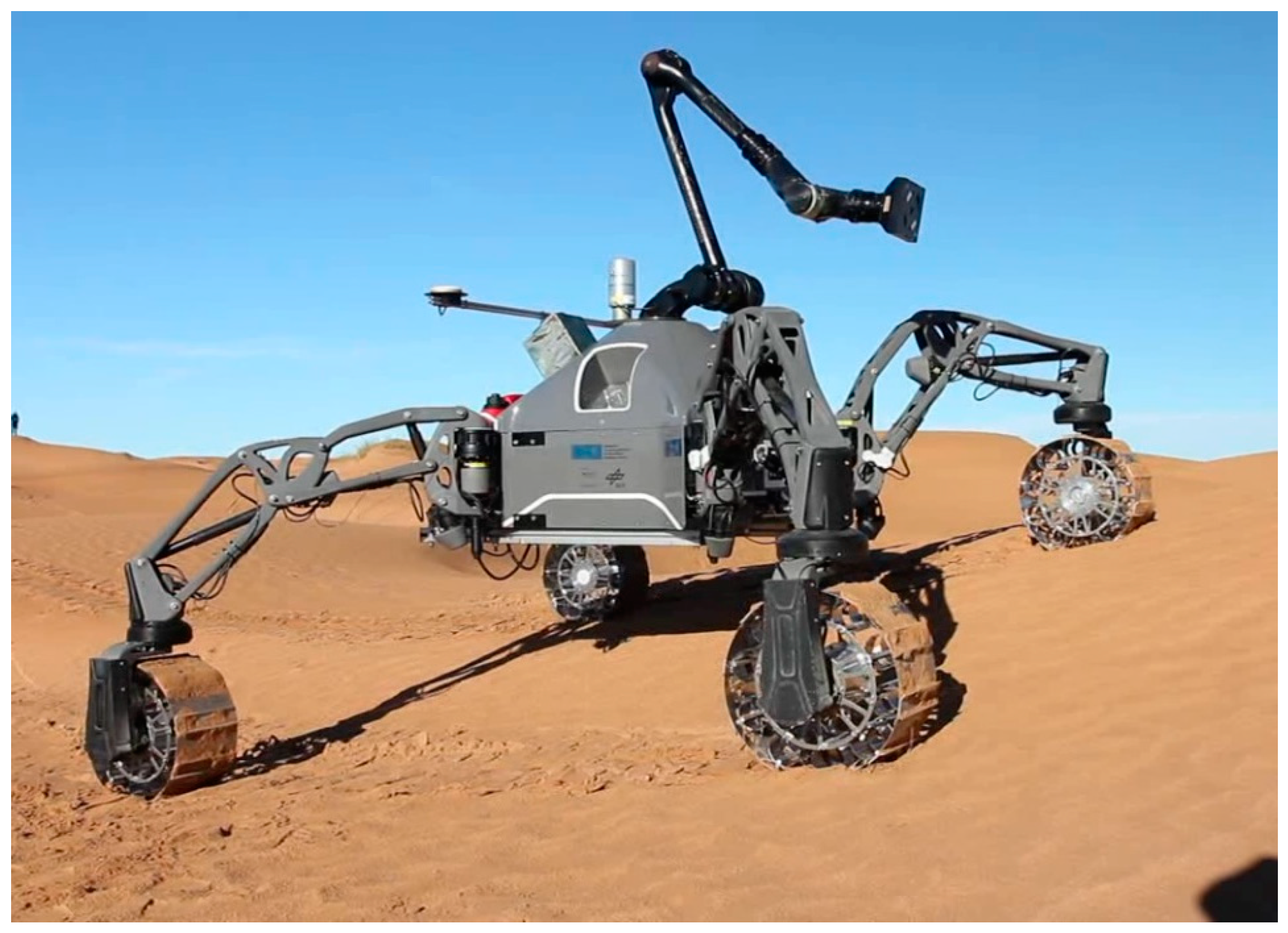
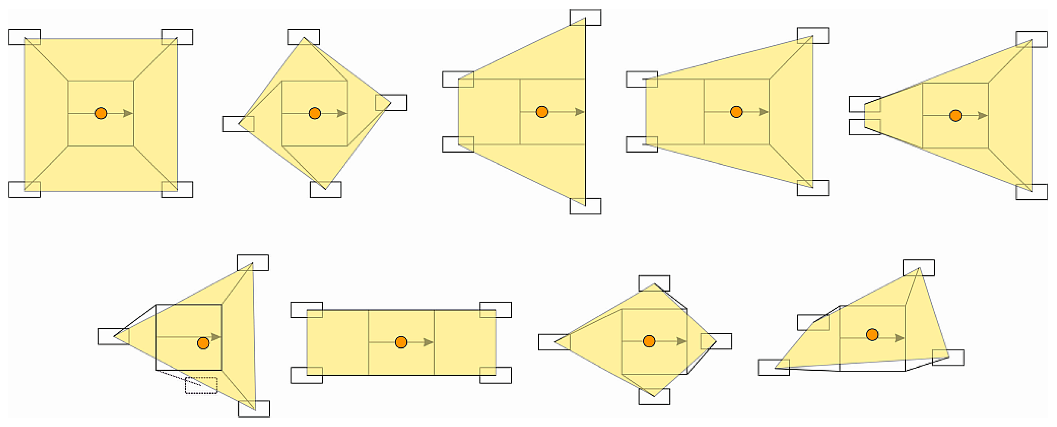
The system is tested and developed using the rover SherpaTT that is shown in Figure 1. SherpaTT was built by DFKI for long-distance exploration applications [26], negotiation of highly challenging terrains or non-nominal conditions (sinkage in soft soil, getting entangled between rocks or alike), cooperation tasks between heterogeneous rovers in a collaborative sample return mission, search and rescue and/or security missions. SherpaTT is a four-wheeled mobile robot [27] outfitted with an actively articulated suspension system, independent drive and steer wheel motors and a six degrees of freedom (DOF) manipulation arm. The rover is also a hybrid wheeled-leg rover, so it can take advantage of both wheeled and legged locomotion according to the terrain difficulty. SherpaTT has a mass of about 166 kg and a payload capacity of at least 80 kg. Each of the four suspended legs has five DOF that include the rotation of the whole leg about the shoulder or pan axis with respect to the robot body, the two rotations of the inner and outer leg parallelograms, the steer and drive angle of the wheel. SherpaTT’s footprint can vary between 1 × 1m in a folded configuration to 2.4 × 2.4 m in a maximum square footprint. Various predefined footprint shapes (stances) can be adopted as explained in Figure 2.
Each of the 20 suspension and six arm joints delivers telemetry data at a rate of 100 Hz. The telemetry includes joint position (absolute and incremental), speed, current, PWM duty cycle and two temperatures (housing and motor windings). Additionally, a 6-DOF force-torque sensor (FTS) is placed at the mounting flange of each wheel-drive actuator enabling the direct measurement of the generalized forces that each wheel exchanges with the supporting surface. Active force control for the wheel-ground contact as well as the roll-pitch adaption are two processes of the so-called Ground Adaption Process (GAP) in SherpaTT [28]. Autonomy modules do not need to cope with the limb articulation in rough terrain [29].
2.1. Data Sets
Two extensive field trials have been conducted by SherpaTT in the desert of Morocco (2019) and in the desert of Utah (2016). Both sites have been shown to be representative of Mars analogue terrain [30]. During these field trials, different test tracks in natural terrain, GAP-modes and footprints have been tested. Since the focus of those campaigns was different from the aim of this research, only a small portion of the data logs can be effectively used for terrain estimation purposes. Table 1 sums up the datasets available for terrain and slippage classification, clarifying specific terrain, total run time and logged sensors. Specifically, the only available run in the Morocco campaign is performed on sandy dunes of flat/moderate slopes, while Utah data logs are available on flat, moderate sloped and steep sloped rocky terrains. Utah moderate sloped terrain presents an inclination less than 10 deg, while steep sloped terrain had a grade up to 28 degrees. All the available experimental runs are performed following a straight path. Sensor signals are logged together with a synchronized timestamp. Four sensor modalities are available on SherpaTT: the four FTSs, the body’s IMU, a Differential Global Positioning System (DGPS) on the rover body and joint telemetry. The FTSs are six axial sensors able to measure the three cartesian components of forces and moments acting on each wheel. The IMU outputs the rover’s attitude ad accelerations, while DGPS provides an absolute position of the rover and it is used for ground truthing. Joint position and speed, as well as each joint’s electrical current and PWM duty cycle, are available for this study.
Proprioceptive data streams have been associated with a sequence of terrain patches with the same length. In this work, a patch length of 0.3 m is considered. In such a way, for each terrain patch, a set of features has been computed, as extensively explained in the following section.
2.2. Data Pre Processing
Each sensor modality could have a different sample rate. Table 2 specifies sensors logging frequencies. The highest frequency is adopted for the definition of a common absolute timestamp: a frequency of 100 Hz corresponding to one observation each of 0.01 s. Signals with lower sample rates are linearly interpolated to obtain signals at 100 Hz.
In order to have the same time–space association logic for all datasets, and since DGPS is not available on Morocco tests, an odometry-based approach is adopted to relate time-stamp with rover traversed distance. The distance travelled by one of the four rover wheels, dV, between two successive time-stamps is defined in Equation (1):
where is the sampling interval, is the wheel angular speed measured by the encoder and is the wheel undeformed radius. Sensor data have been subdivided into sub-logs that are associated with each virtual patch. It should be noted that two patches of the same length, in general, may correspond to different actual travel distances due to the extent of wheel slippage. It is also worth mentioning that the use of “distance” windows is used under the underlying assumption of continuous motion of the robot without any stop-and-go manoeuvre.
3. Proprioceptive Sensing
This section presents the set of proprioceptive features used to characterize the properties of a given terrain patch. For each feature, the four statistical moments (mean, variance, skewness and kurtosis) are computed. Data have been manually labelled in terms of two terrain types (sand for Morocco and rocky terrain for Utah) and in terms of three discrete classes of slippage (only for Utah, where slippage can be directly calculated by comparing DGPS with wheel encoders). Data labelling is necessary, as explained later, for the successive stages of feature selection using validity indices and for training the terrain and slippage classifiers.
3.1. Proprioceptive Features
A large amount of sensory data can be gathered from Sherpa and potentially used for classification purposes. However, only a few signals bring significant information related to terrain type. Here, only the most relevant features that we found are discussed. From the FTSs, three forces and three moments are available for each wheel. Among these, we retain the longitudinal force FX and the wheel drive torque TD. The wheel drive torque can be also estimated indirectly from the electrical current, CD, whereas the wheel angular velocity ω can be obtained from wheel encoders. The three body accelerations ax, ay and az are estimated from the IMU. The mechanical power PM and the electrical power PE are computed, respectively, in Equations (2) and (3):
where V, I and dPWM are, respectively, the motor voltage, current and PWM duty cycle of the wheel drive. Apart from this set of “primary” quantities, a second set of “derivate” features has been found to be effective for terrain characterization. Derivate features can be obtained by combining primary features according to well-known physics-based relationships. As an example, the friction coefficients μ can be estimated using three different sensor data according to Equations (4)–(6):
where FZ is the wheel vertical force and R is the wheel unloaded radius. Another key feature is the so-called wheel speed deviation, SD, that is the absolute value of the difference between the angular speed of each wheel ω and the average angular speed of the four wheels as defined by Equation (7):
Note that the SD can be extended as well to turning motion, as explained in [31]. Wheel longitudinal stiffness LS is computed as the ratio between the friction coefficient and the wheel slip s. In the simplified case of a linear relation between friction coefficient and wheel slip, this physical quantity should represent the slope of friction—slippage plot. Three different LSi values are computed in Equation (8) using the three friction coefficients defined before:
The slippage s is univocally estimated for both accelerating and braking and for each wheel based on Equation (9):
where VX is estimated with the DGPS and d is positive for accelerating and negative for braking. An approximate estimate of wheel sinkage z can be obtained by Equation (10) [32]:
Table 3 sums up the proprioceptive feature space spanned by the above considerations.
3.2. Statistical Feature and Validity Indices
For the i-th feature, the main statistical moments are estimated: mean , variance , skewness and kurtosis of the feature signal for a single terrain patch. These statistics are defined according to Equations (11)–(14):
where is the value assumed by the feature at the time-step and is the total number of time-steps for the considered terrain patch.
In addition, each terrain patch is labelled for terrain type, sand for Morocco data or rock for Utah data, and slippage level; high slip is for absolute value of slip greater than 0.5 and all other conditions are low slip.
The statistical features are divided into clusters according to patch labels and a validity index value is associated with each statistical feature. Two validity indices are proposed to obtain a quantitative measure of “feature goodness” for terrain patch classification: the WB index [33] and a Pearson Coefficient based index (PC) [34]. These indices are employed in the feature selection method described in the following section. The WB index is computed as:
The sum of square within cluster SSW and between clusters SSB can be computed as follows:
where xi is the generic statistical feature value for the patch i, μk is the cluster k centroid value, μ is the overall dataset centroid value, nk is the number of patches in the cluster k and m is the number of clusters. In this study m is 2 since we have two classes for the terrain classifier. WB index assumes lower values for higher distance between different cluster centroids and for lower variance within clusters. A good classifier feature allows us to obtain distant and compact clusters, and thus generally corresponds to a low value of the WB index. A PC index could be computed through the linear regression of a feature against the m classes, giving a progressive numerical value to each class. A higher value of PC potentially corresponds to a better classifier feature.
3.3. Feature Selection
In a classification problem, plenty of features can be thought of and used for training. Features can be raw data signals, or a combination of raw signals, signal statistics and so on. However, only a small amount of the available feature set may be actually relevant to address the classification problem.
The selection of the “most significant features” can be tackled in different ways, i.e., as an optimization or a search problem [34]. Those techniques can find a local or global optimum feature set but could be also computationally expensive. The method proposed in this work has a low computational cost, since the number of its iterations equals the total number of features in the initial feature space. For the purpose of this work the initial feature space is made up of 15 features and 4 statistics per feature, for a total number of 60 statistical features.
The feature selection method needs as input the labelled initial feature space, the value of a validity index (VI) associated with each statistical feature and a classifier to be iteratively trained. The VIs employed in this research were the WB index and the PC index. The classification algorithm is a linear Support Vector Machine (SVM), one of the most adopted techniques for terrain classification problem [18], which guarantees good results with a lower computational effort compared with other techniques such as Convolutional Neural Networks [35]. The feature selection algorithm is described by the following pseudo-code:
- 01.
- INPUT: initial feature set (Ifs), VI vector associated with features VIv
- 02.
- arrangeIFs features in decreasing order of VIv
- 03.
- initialize(F1 score)i−1= 60%, initialize reduced feature set (RFs) as an empty set
- 04.
- forifrom 1 to (number of features)
- 05.
- add the i feature from IFs to the RFs
- 06.
- trainn times the classifier, compute average (F1 score)i
- 07.
- if(F1 score)i − (F1 score)i−1 ≤ (F1 threshold)
- 08.
- removei feature from RFs
- 09.
- end if
- 10.
- update(F1 score)i = (F1 score)i−1
- 11.
- end for
- 12.
- OUTPUT: RFs
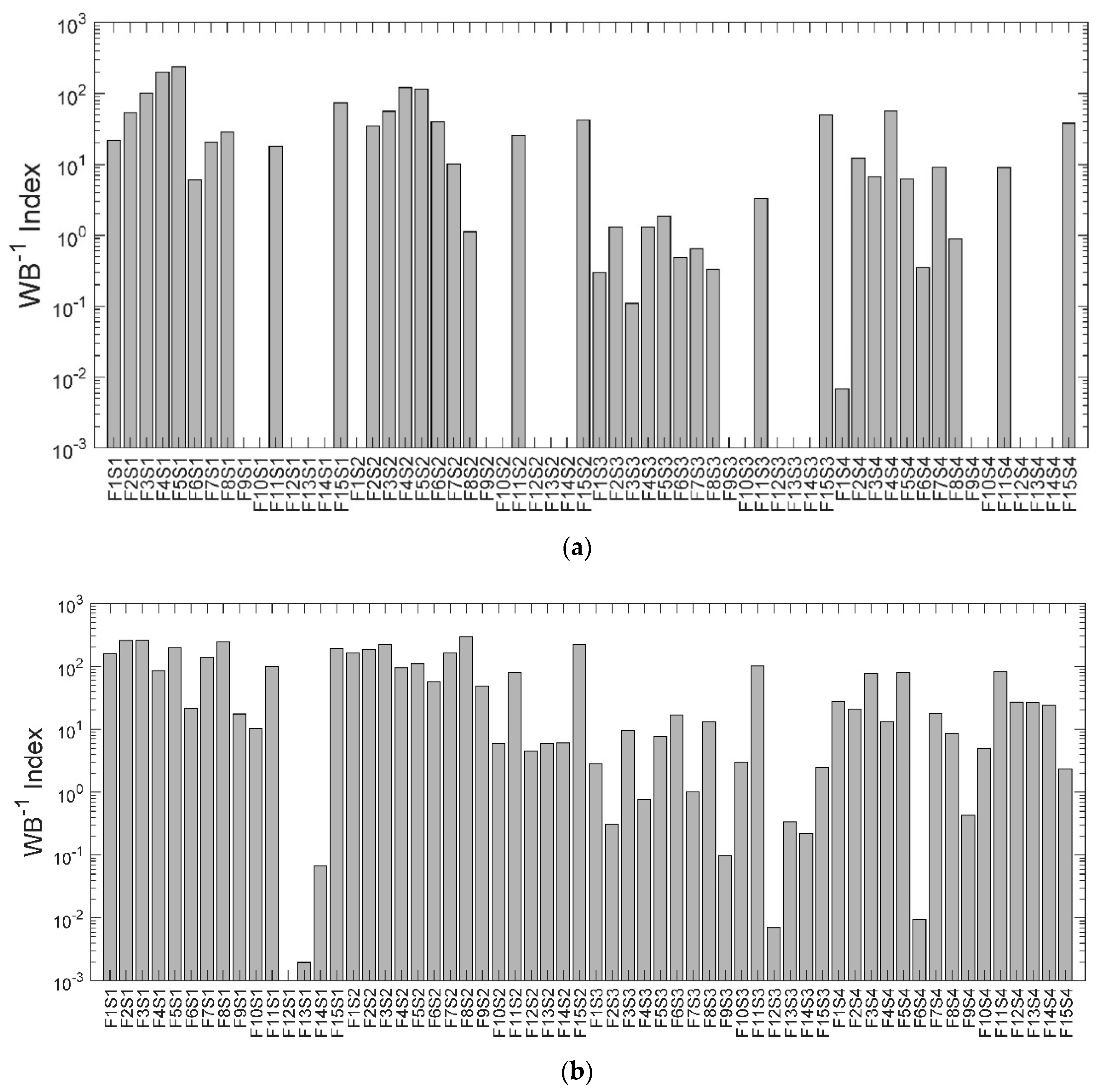
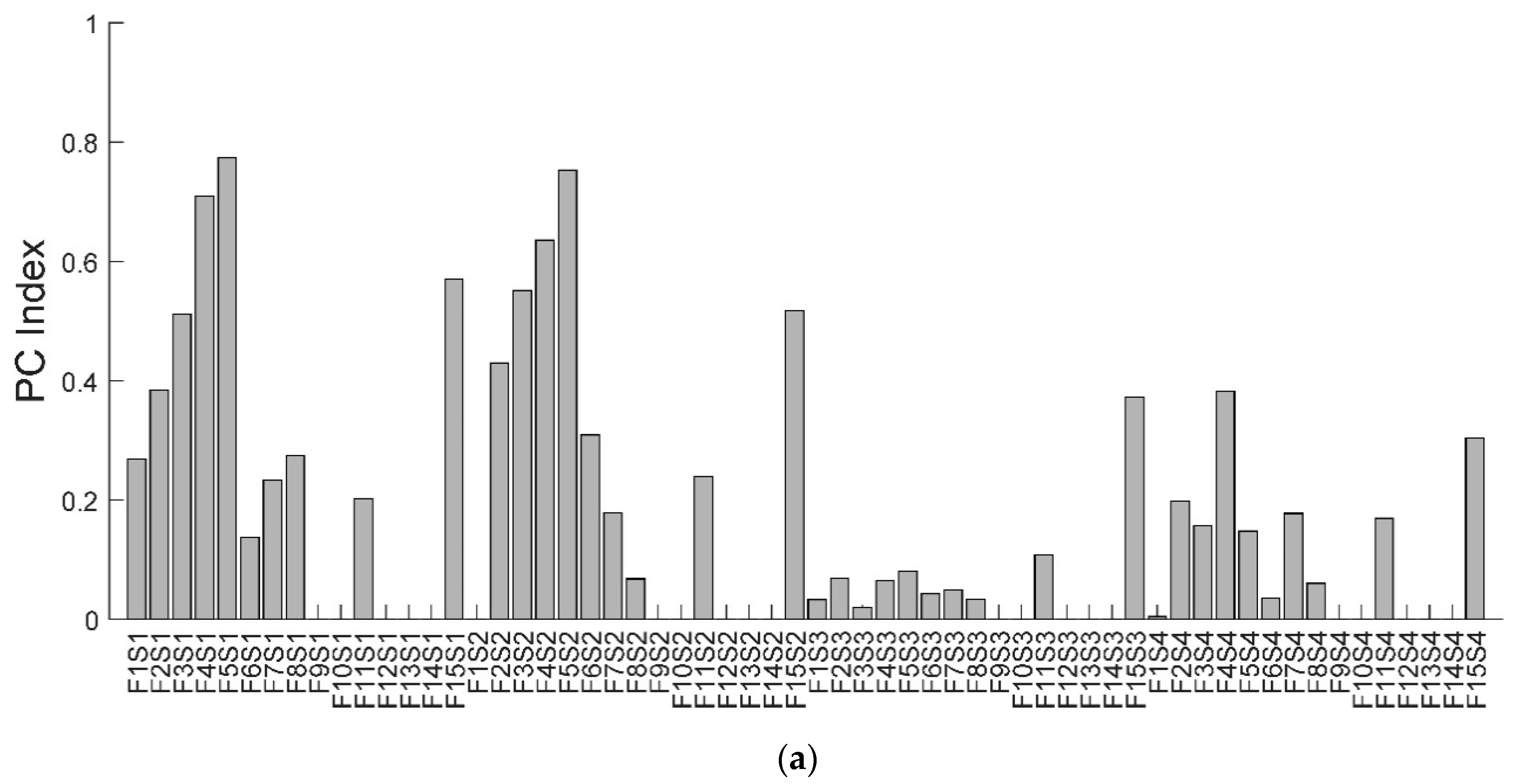
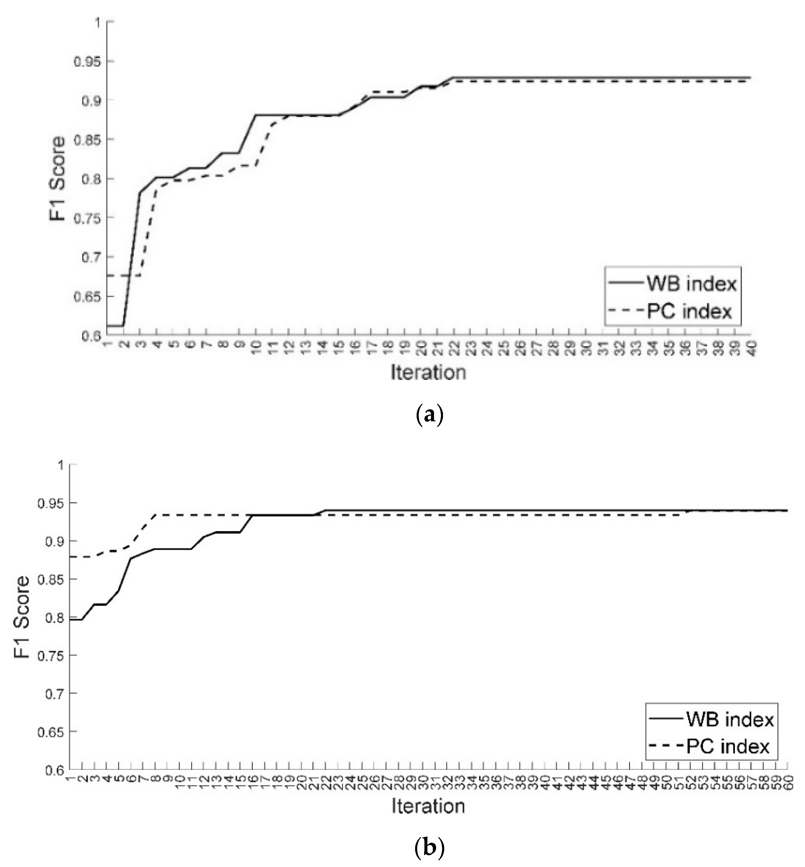
At each iteration step, a feature is added to the training set and the algorithm verifies if this new feature leads to a significant increase in the classifier performance. The metric used to quantify the classifier performance is the F1 score. In this work the F1 score percentage improvement threshold for a feature to be accepted has been set to 0.5%. The training phase is repeated three times for each feature (n = 3) and an average F1 score of the three trained classifiers is computed. The output of the algorithm is a reduced feature set, including the only features that bring a significant improvement in the classifier performance. The algorithm has been tested both with the PC index and the reciprocal of WB index (), which allows the first selected features to be potentially the most suitable for the classifier. Figure 5 shows the algorithm results in terms of F1 score for each iteration and for the terrain (above) and slippage (below) classifier. If the performance increase, the new feature is added to the “optimal” or reduced feature set (RFs). It is apparent how the most relevant features are found in the first half of the iterations, where both PC and WB−1 have higher values. This figure shows that the chosen validity indices are effective for the selection of relevant features.
Table 4 and Table 5 show the F1 score and the number of selected features for the terrain classifier and for different feature selection methods. PC and WB indicate the feature selection method that uses the singular VI, as described before. In addition, two combined selections have been also tested that use the intersection and the union of the selected feature set obtained from the and selection method. Finally, the training method “All” involves the use of the entire feature set.
All the proposed selection methods for the terrain classifier achieve similar F1 score of about 93%. However, the intersection method Int(PC,WB) is the most suitable both for the F1 score and the size of the reduced feature set. Both single VI methods lead also to similar reduced feature sets. In fact, nine of the features selected by both WB and PC methods fall into the intersection Int(PC,WB). Taking all initial features (see “All” method), without any selection phase allows us to reach a good F1 score of 90.4%, but with a higher training set dimensionality and so a higher computational effort.
The same selection procedure has been performed with the slippage classifier. PC and WB methods select different features. The most relevant features fall into the intersection, which has a slightly lower F1 but a minimal feature set, hence it can be preferred as the selection method. Table 6 collects the reduced feature space for both algorithms.
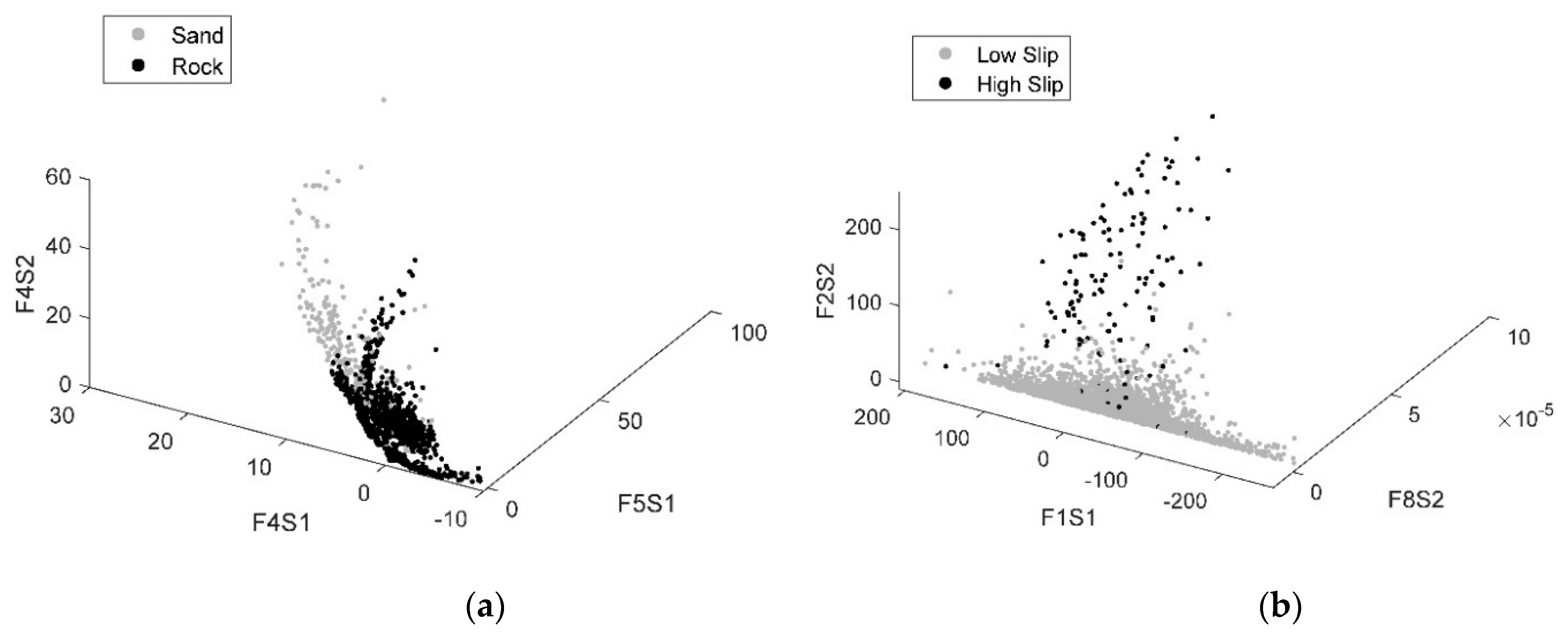
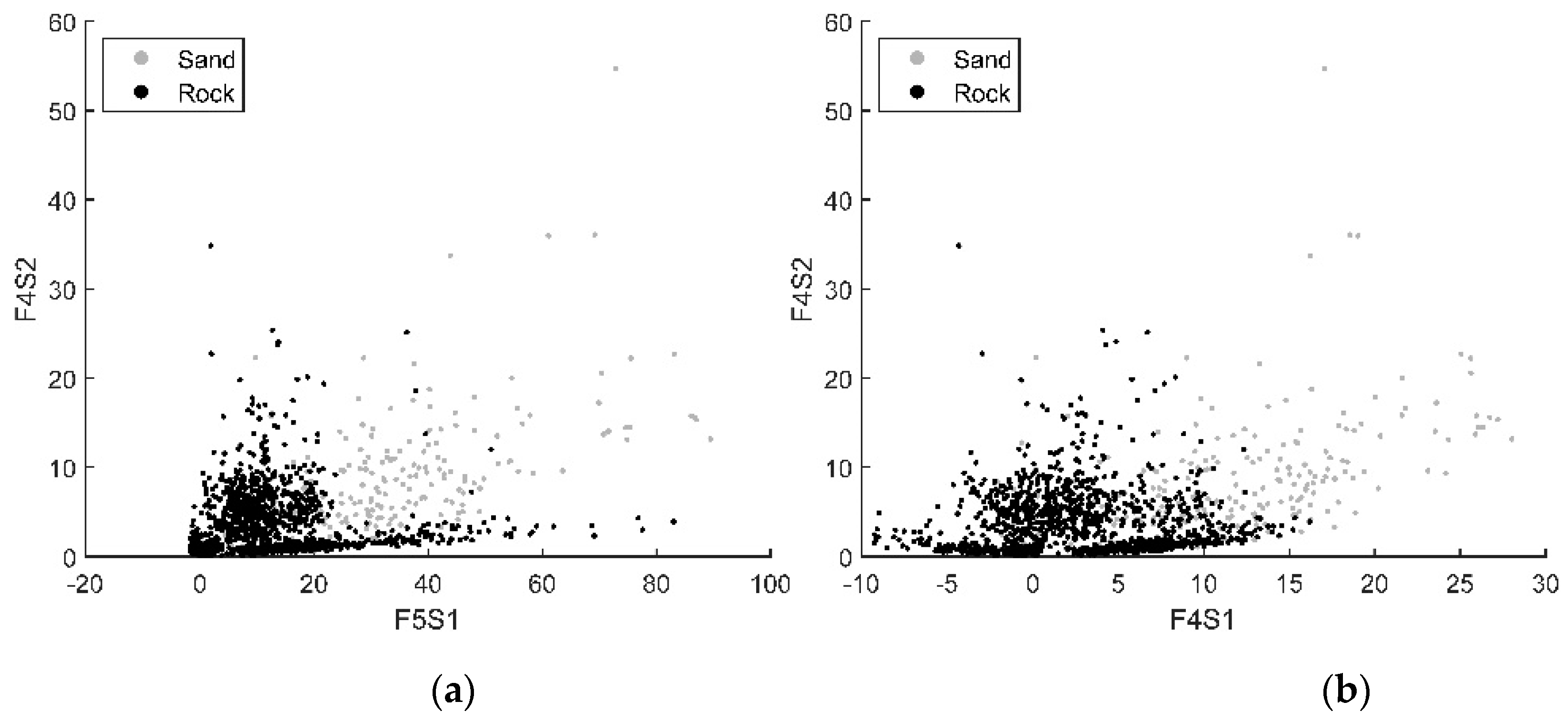
Figure 6 shows the 3D scatter plot of the three statistical features that present the highest value of WB and PC index, respectively, for the terrain and high-slippage classifier. For visualization purposes and for the terrain classifier only, the corresponding 2D feature distribution is also shown in Figure 7. As seen from these figures, the feature distribution indicates a good separation level between sand and rock and it suggests the implementation of a classification algorithm.
4. Classification Task
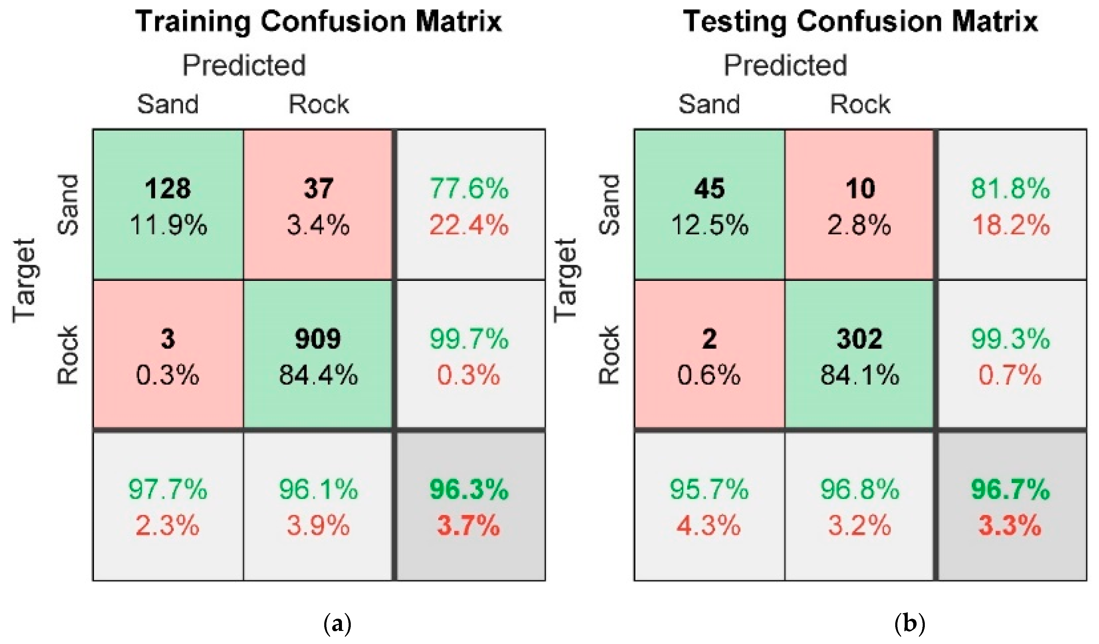
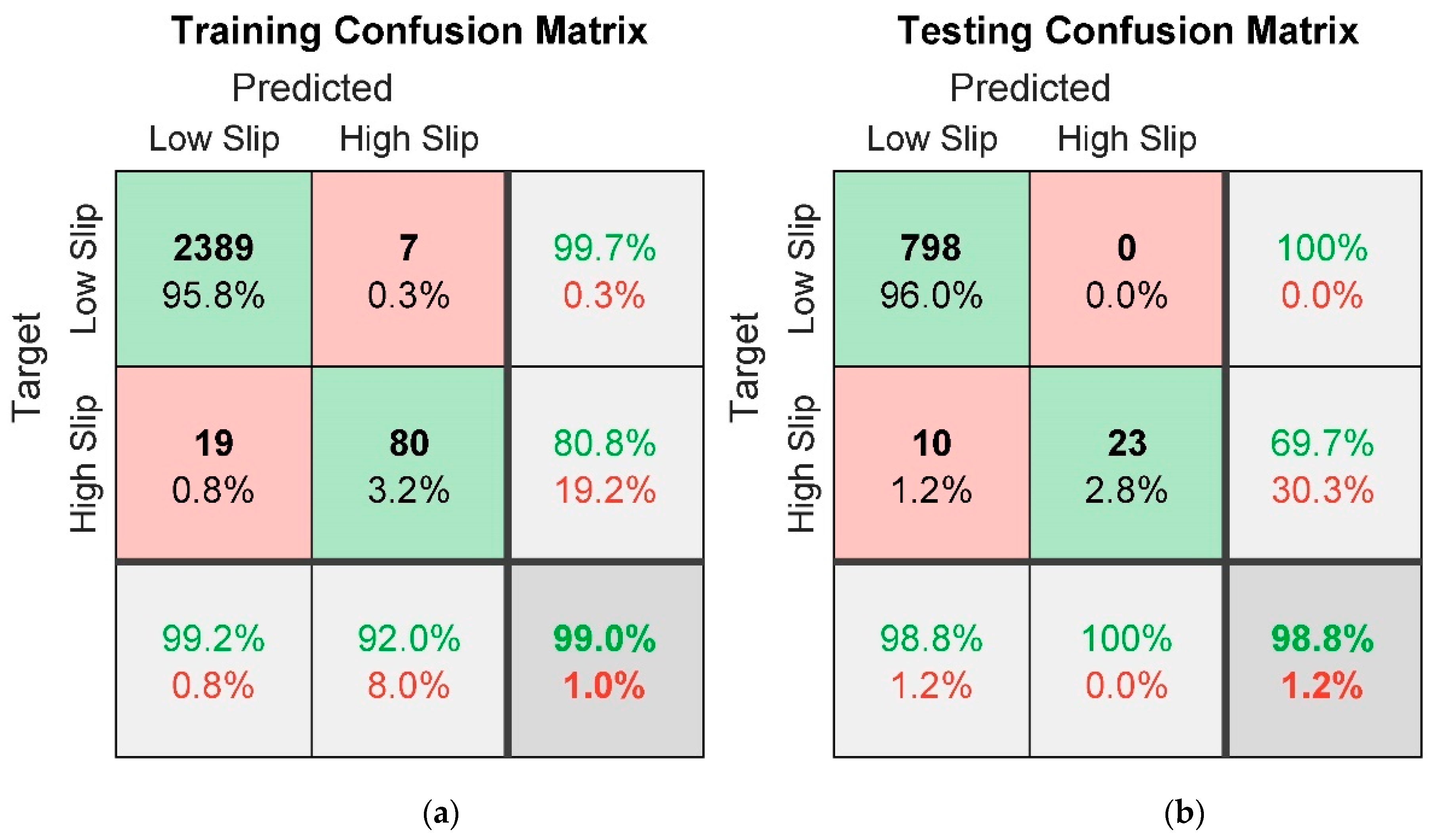
In this section, the results obtained from the two classifiers for terrain and slippage detection are presented. The classifiers were trained and tested on real data gathered by SherpaTT in the field. The reduced feature sets to be used for training and testing have been obtained with the intersection method described in the previous section (refer to Table 6). For both classifiers, the observations (terrain patches) of the reduced feature dataset have been subdivided into two datasets, according to the patch class. In addition, 75% of the observations of each class dataset were randomly extracted to build the training datasets, while the remaining 25% were then used for testing the trained classifiers [36]. Table 7 and Table 8 show the performance metrics of the trained classifiers. The terrain classifier reaches a global accuracy of 96.3% and a global F1 score of 92.2%, while the slippage classifier has an accuracy of 99.0% and an F1 score of 92.7%.
5. Discussion and Conclusions
A general approach for terrain and slippage classification has been proposed and validated through field experimental data. A SherpaTT rover testing campaign performed in Morocco and Utah deserts provided proprioceptive datasets on different soil types. A set of features have been defined and extracted from raw experimental data. Two labels for terrain type (Sand–Rock) and slippage level (High Slip–Low Slip) have been associated with each terrain patch, together with a set of statistical features (predictors), obtained from the computation of feature statistical moments on the terrain patch. Different selection methods based on validity index have been tested and proved to be effective for the extraction of relevant features. Different selection methods based on validity index have been tested. The tested validity indices are the WB index and a Pearson Coefficient (PC)-based index. Both indices are demonstrated to be effective for the extraction of relevant features. Only the features selected by both WB and PC methods have been kept in the reduced feature set used for classifiers training and testing. Thanks to the selection, the initial statistical feature set of 60 features was reduced to 9 features and to 2 features for slippage classification. The reduced feature set observations, one per terrain patch, were randomly subdivided into a training set and a testing set, including, respectively, 75% and 25% of the observations. The two classifiers were trained on the training set and then tested on the new samples of the testing set, giving as result a global classifier accuracy of 96.7% for terrain classification and 98.8% for slippage classification.
New experimental tests will be performed in the near future on different terrain types and during various rover maneuvers. Those new data will be used to further validate the proposed approach and to improve the classifier generalization. The combination of proprioceptive sensing with exteroceptive perception, as suggested in [18], will be also investigated.
Author Contributions
Conceptualization, M.D., G.R.; Methodology, M.D., G.R.; Data curation and experiments and validation, F.C.; writing—original draft preparation, M.D, G.R.; writing—review and editing, F.C. All authors have read and agreed to the published version of the manuscript.
Funding
This research was funded by the Horizon 2020 European Commission under grant agreement n. 821988 ADE.
Conflicts of Interest
The authors declare no conflict of interest.
References
- Gonzalez, R.; Iagnemma, K. Slippage estimation and compensation for planetary exploration rovers. State of the art and future challenges. J. Field Robot. 2017, 35, 564–577. [Google Scholar] [CrossRef]
- Filip, J.; Azkarate, M.; Visentin, G. Trajectory Control for Autonomous Planetary Rovers. In Proceedings of the Symposium on Advanced Space Technologies in Automation and Robotics, Leiden, The Netherlands, 20–22 June 2017; pp. 1–6. [Google Scholar]
- Reina, G.; Ishigami, G.; Nagatani, K.; Yoshida, K. Odometry Correction Using Visual Slip Angle Estimation for Planetary Exploration Rovers. Adv. Robot. 2010, 24, 359–385. [Google Scholar] [CrossRef]
- Ojeda, L.; Reina, G.; Cruz, D.; Borenstein, J. The FLEXnav precision dead-reckoning system. Int. J. Veh. Auton. Syst. 2006, 4, 173. [Google Scholar] [CrossRef] [Green Version]
- Bussmann, K.; Meyer, L.; Steidle, F.; Wedler, A. Slip Modeling and Estimation for a Planetary Exploration Rover: Experimental Results from Mt. Etna. In Proceedings of the 2018 IEEE/RSJ International Conference on Intelligent Robots and Systems (IROS), Madrid, Spain, 1–5 October 2018; pp. 2449–2456. [Google Scholar]
- Sanguino, T.D.J.M. 50 years of rovers for planetary exploration: A retrospective review for future directions. Robot. Auton. Syst. 2017, 94, 172–185. [Google Scholar]
- Goldberg, S.B.; Maimone, M.; Matthies, L. Stereo vision and rover navigation software for planetary exploration. In Proceedings of the IEEE Aerospace Conference; Institute of Electrical and Electronics Engineers (IEEE), Big Sky, MT, USA, 8–15 March 2003. [Google Scholar]
- Helmick, D.; Angelova, A.; Matthies, L. Terrain Adaptive Navigation for planetary rovers. J. Field Robot. 2009, 26, 391–410. [Google Scholar] [CrossRef] [Green Version]
- Gingras, D.; Lamarche, T.; Bedwani, J.-L.; Dupuis, É. Rough Terrain Reconstruction for Rover Motion Planning. In Proceedings of the 2010 Canadian Conference on Computer and Robot Vision, Ottawa, ON, Canada, 31 May–2 June 2010; pp. 191–198. [Google Scholar]
- Thrun, S.; Montemerlo, M.; Dahlkamp, H.; Stavens, D.; Aron, A.; Diebel, J.; Fong, P.; Gale, J.; Halpenny, M.; Hoffmann, G.; et al. Stanley: The Robot that Won the DARPA Grand Challenge. J. Field Robot. 2006, 23, 661–692. [Google Scholar] [CrossRef]
- Milella, A.; Reina, G.; Underwood, J.; Douillard, B. Combining radar and vision for self-supervised ground segmentation in outdoor environments. In Proceedings of the IEEE International Conference on Intelligent Robots and Systems, San Francisco, CA, USA, 25–30 September 2011; pp. 255–260. [Google Scholar]
- Milella, A.; Reina, G.; Underwood, J.; Douillard, B. Visual ground segmentation by radar supervision. Robot. Auton. Syst. 2014, 62, 696–706. [Google Scholar] [CrossRef]
- Bekker, M. The development of a moon rover. J. Br. Interpl. Soc. 1985, 38, 537. [Google Scholar]
- Angelova, A.; Matthies, L.; Helmick, D.; Perona, P. Learning and prediction of slip from visual information. J. Field Robot. 2007, 24, 205–231. [Google Scholar] [CrossRef]
- Gonzalez, R.; Chandler, S.; Apostolopoulos, D. Characterization of machine learning algorithms for slippage estimation in planetary exploration rovers. J. Terramech. 2019, 82, 23–34. [Google Scholar] [CrossRef]
- Reina, G.; Leanza, A.; Messina, A. On the vibration analysis of off-road vehicles: Influence of terrain deformation and irregularity. J. Vib. Control. 2018, 24, 5418–5436. [Google Scholar] [CrossRef]
- Valada, A.; Burgard, W. Deep spatiotemporal models for robust proprioceptive terrain classification. Int. J. Robot. Res. 2017, 36, 1521–1539. [Google Scholar] [CrossRef] [Green Version]
- Reina, G.; Milella, A.; Galati, R. Terrain assessment for precision agriculture using vehicle dynamic modelling. Biosyst. Eng. 2017, 162, 124–139. [Google Scholar] [CrossRef]
- Brooks, C.A.; Iagnemma, K. Self-supervised terrain classification for planetary surface exploration rovers. J. Field Robot. 2012, 29, 445–468. [Google Scholar] [CrossRef]
- Krebs, A.; Pradalier, C.; Siegwart, R. Adaptive rover behavior based on online empirical evaluation: Rover–terrain interaction and near-to-far learning. J. Field Robot. 2010, 27, 158–180. [Google Scholar] [CrossRef]
- Dupont, E.M.; Moore, C.A.; Collins, E.G.; Coyle, E.; Collins, E.G. Frequency response method for terrain classification in autonomous ground vehicles. Auton. Robot. 2008, 24, 337–347. [Google Scholar] [CrossRef]
- Reina, G.; Leanza, A.; Messina, A. Terrain estimation via vehicle vibration measurement and cubature Kalman filtering. J. Vib. Control. 2019, 26, 885–898. [Google Scholar] [CrossRef]
- Iagnemma, K.; Kang, S.; Shibly, H.; Dubowsky, S. Online Terrain Parameter Estimation for Wheeled Mobile Robots with Application to Planetary Rovers. IEEE Trans. Robot. 2004, 20, 921–927. [Google Scholar] [CrossRef] [Green Version]
- Gallina, A.; Krenn, R.; Scharringhausen, M.; Uhl, T.; Schafer, B. Parameter Identification of a Planetary Rover Wheel-Soil Contact Model via a Bayesian Approach. J. Field Robot. 2013, 31, 161–175. [Google Scholar] [CrossRef] [Green Version]
- Dimastrogiovanni, M.; Cordes, F.; Reina, G. Terrain Sensing for Planetary Rovers. In Proceedings of the International Conference of IFToMM ITALY, Naples, Italy, 9–11 September 2020; pp. 269–277. [Google Scholar]
- Cordes, F.; Dettmann, A.; Kirchner, F. Locomotion modes for a hybrid wheeled-leg planetary rover. In Proceedings of the 2011 IEEE International Conference on Robotics and Biomimetics, Phuket, Thailand, 7–11 December 2011; pp. 2586–2592. [Google Scholar]
- Sonsalla, R.U.; Cordes, F.; Christensen, L.; Roehr, T.M.; Stark, T.; Planthaber, S.; Maurus, M.; Mallwitz, M.; Kirchner, E.A. Field Testing of a Cooperative Multi-Robot Sample Return Mission in Mars Analogue Environment. In Proceedings of the 14th Symposium on Advanced Space Technologies in Robotics and Automation (ASTRA’17), Noordwijk, The Netherlands, 27–28 May 2017. [Google Scholar]
- Cordes, F.; Kirchner, F.; Babu, A. Design and field testing of a rover with an actively articulated suspension system in a Mars analog terrain. J. Field Robot. 2018, 35, 1149–1181. [Google Scholar] [CrossRef]
- Cordes, F.; Babu, A.; Kirchner, F. Static force distribution and orientation control for a rover with an actively articulated suspension system. In Proceedings of the 2017 IEEE/RSJ International Conference on Intelligent Robots and Systems (IROS), Vancouver, BC, Canada, 24–28 September 2017; pp. 5219–5224. [Google Scholar]
- Clarke, J.; Stoker, C.R. Concretions in exhumed and inverted channels near Hanksville Utah: Implications for Mars. Int. J. Astrobiol. 2011, 10, 161–175. [Google Scholar] [CrossRef]
- Reina, G. Cross-Coupled Control for All-Terrain Rovers. Sensors 2013, 13, 785–800. [Google Scholar] [CrossRef] [PubMed] [Green Version]
- Guo, J.; Guo, T.; Zhong, M.; Gao, H.; Huang, B.; Ding, L.; Li, W.; Deng, Z. In-situ evaluation of terrain mechanical parameters and wheel-terrain interactions using wheel-terrain contact mechanics for wheeled planetary rovers. Mech. Mach. Ther. 2020, 145, 103696. [Google Scholar] [CrossRef]
- Zhao, Q.; Fränti, P. WB-index: A sum-of-squares based index for cluster validity. Data Knowl. Eng. 2014, 92, 77–89. [Google Scholar] [CrossRef]
- Hastie, T.; Tibshirani, R.; Friedman, J. The Elements of Statistical Learning; Springer: New York, NY, USA, 2009. [Google Scholar]
- Rothrock, B.; Kennedy, R.; Cunningham, C.; Papon, J.; Heverly, M.; Ono, M. SPOC: Deep Learning-based Terrain Classification for Mars Rover Missions. In Proceedings of the AIAA SPACE 2016, Long Beach, CA, USA, 13–16 September 2016. [Google Scholar]
- Milella, A.; Marani, R.; Petitti, A.; Reina, G. In-field high throughput grapevine phenotyping with a consumer-grade depth camera. Comput. Electron. Agric. 2019, 156, 293–306. [Google Scholar] [CrossRef]
Figure 1.
SherpaTT in soft sand dunes during Morocco field trials in 2018.

Figure 2.
Examples of possible footprint configurations and resulting support polygons.

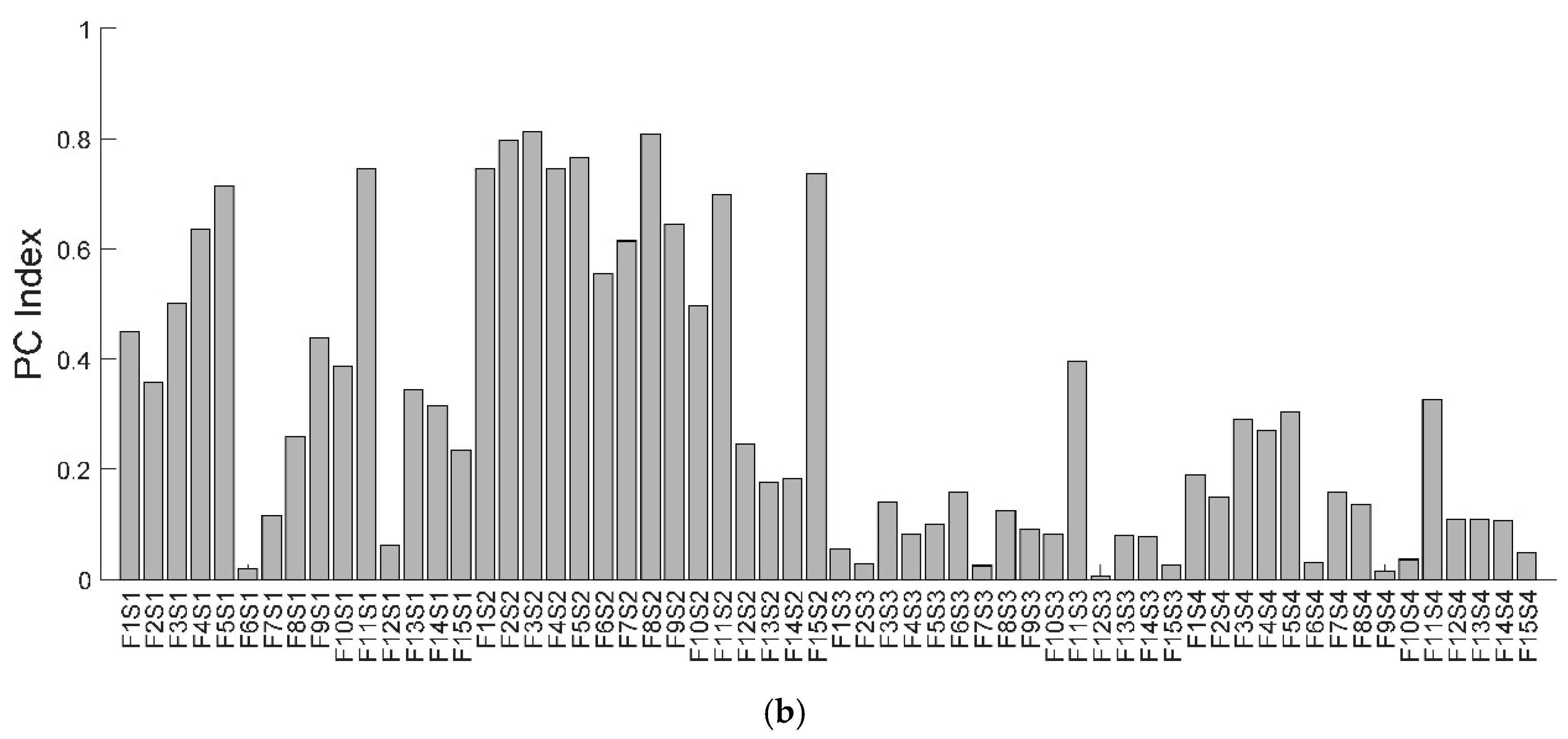
Figure 3.
index values for each feature (F1 to F15), for each statistic (S1 to S4, respectively, mean, variance, skewness and kurtosis) and for terrain (a) and slippage (b) classifier.
Figure 3.
index values for each feature (F1 to F15), for each statistic (S1 to S4, respectively, mean, variance, skewness and kurtosis) and for terrain (a) and slippage (b) classifier.

Figure 4.
index values for each feature (F1 to F15), for each statistic (S1 to S4, respectively, mean, variance, skewness and kurtosis) and for terrain (a) and slippage (b) classifier.
Figure 4.
index values for each feature (F1 to F15), for each statistic (S1 to S4, respectively, mean, variance, skewness and kurtosis) and for terrain (a) and slippage (b) classifier.


Figure 5.
Feature selection performance results for terrain (a) and slippage (b) classifier.

Figure 6.
3D plot of the first three most relevant features selected for terrain (a) and slippage (b) classification.
Figure 6.
3D plot of the first three most relevant features selected for terrain (a) and slippage (b) classification.

Figure 7.
2D distribution of the most relevant features selected for the terrain classifier: F4S2-F5S1 plane (a), F4S2-F4S1 plane (b).
Figure 7.
2D distribution of the most relevant features selected for the terrain classifier: F4S2-F5S1 plane (a), F4S2-F4S1 plane (b).

Figure 8.
Confusion matrix for training (a) and testing (b) of the terrain classifier.

Figure 9.
Confusion matrix for training (a) and testing (b) of the slippage classifier.


Table 1.
Datasets gathered by SherpaTT during field trials; for each test run, terrain description, testing time and available logged sensors are indicated.
Table 1.
Datasets gathered by SherpaTT during field trials; for each test run, terrain description, testing time and available logged sensors are indicated.
| Run ID | Test Site | Terrain Type | Slope | Run Time [s] | FTS | IMU | DGPS | Encoders |
|---|---|---|---|---|---|---|---|---|
| R01 | Morocco | Sand | Flat/Moderate | 381.5 | ✓ | ✗ | ✗ | ✓ |
| R02 | Utah | Rock | Flat | 214.8 | ✓ | ✓ | ✓ | ✓ |
| R03 | Utah | Rock | Flat | 214.8 | ✓ | ✓ | ✓ | ✓ |
| R04 | Utah | Rock | Moderate | 152.4 | ✓ | ✓ | ✗ | ✓ |
| R05 | Utah | Rock | Steep | 453.9 | ✓ | ✓ | ✓ | ✓ |
| R06 | Utah | Rock | Steep | 457.7 | ✓ | ✓ | ✓ | ✓ |
| R07 | Utah | Rock | Steep | 481.2 | ✓ | ✓ | ✓ | ✓ |
Table 2.
Sensor sample rates.
| Sensor Modality | Sample Rate [Hz] |
|---|---|
| FTS | 100 |
| IMU | 100 |
| DGPS | 10–20 |
| Encoders | 100 |
Table 3.
Proprioceptive features with relative feature ID number and symbol.
| FID | Feature | Symbol |
|---|---|---|
| F1 | Longitudinal Force | |
| F2 | Drive Torque | |
| F3 | Drive Current | |
| F4 | Mechanical Power | |
| F5 | Electrical Power | |
| F6 | Friction Coefficient 1 | |
| F7 | Friction Coefficient 2 | |
| F8 | Friction Coefficient 3 | |
| F9 | Acceleration X | |
| F10 | Acceleration Z | |
| F11 | Speed Deviation | |
| F12 | Longitudinal Stiffness 1 | |
| F13 | Longitudinal Stiffness 2 | |
| F14 | Longitudinal Stiffness 3 | |
| F15 | Sinkage |
Table 4.
Comparison of different feature selection methods for terrain classification.
| N° features | 11 | 10 | 9 | 12 | 40 |
| F1 score | 0.924 | 0.929 | 0.931 | 0.928 | 0.904 |
Table 5.
Comparison of different feature selection methods for slippage classification.
| N° features | 6 | 10 | 2 | 14 | 60 |
| F1 score | 0.939 | 0.940 | 0.914 | 0.936 | 0.765 |
Table 6.
Reduced feature sets for terrain (a) and slippage (b) classification.
| F5S1 | F5S1 | F2S1 | F1S1 |
| F4S1 | F4S1 | F3S1 | F2S1 |
| F4S2 | F4S2 | F4S1 | F3S1 |
| F3S2 | F3S1 | F5S1 | F4S1 |
| F3S1 | F4S4 | F8S1 | F5S1 |
| F2S1 | F2S1 | F11S1 | F8S1 |
| F4S4 | F8S1 | F4S2 | F11S1 |
| F8S1 | F11S2 | F7S2 | F3S2 |
| F1S1 | F11S1 | F4S4 | F4S2 |
| F11S1 | F7S2 | F7S2 | |
| F7S2 | F11S2 | ||
| F4S4 | |||
| F3S2 | F8S2 | F1S2 | F1S1 |
| F2S2 | F3S1 | F3S2 | F3S1 |
| F4S2 | F8S1 | F5S1 | |
| F1S2 | F3S2 | F8S1 | |
| F11S1 | F15S2 | F11S1 | |
| F1S3 | F5S1 | F1S2 | |
| F1S2 | F2S2 | ||
| F1S1 | F3S2 | ||
| F11S3 | F4S2 | ||
| F11S2 | F8S2 | ||
| F11S2 | |||
| F15S2 | |||
| F1S3 | |||
| F11S3 |
Table 7.
Performance metrics of the terrain classifier.
| Precision | Recall | Specificity | F1 Score | |
|---|---|---|---|---|
| Sand | 77.6% | 97.7% | 96.1% | 86.5% |
| Rock | 99.7% | 96.1% | 97.7% | 97.9% |
Table 8.
Performance metrics of the slippage classifier.
| Precision | Recall | Specificity | F1 Score | |
|---|---|---|---|---|
| Low slip | 99.7% | 99.2% | 92.0% | 99.5% |
| High slip | 80.8% | 92.0% | 99.2% | 86.0% |
© 2020 by the authors. Licensee MDPI, Basel, Switzerland. This article is an open access article distributed under the terms and conditions of the Creative Commons Attribution (CC BY) license (http://creativecommons.org/licenses/by/4.0/).
Share and Cite
MDPI and ACS Style
Dimastrogiovanni, M.; Cordes, F.; Reina, G. Terrain Estimation for Planetary Exploration Robots. Appl. Sci. 2020, 10, 6044. https://0-doi-org.brum.beds.ac.uk/10.3390/app10176044
AMA Style
Dimastrogiovanni M, Cordes F, Reina G. Terrain Estimation for Planetary Exploration Robots. Applied Sciences. 2020; 10(17):6044. https://0-doi-org.brum.beds.ac.uk/10.3390/app10176044
Chicago/Turabian StyleDimastrogiovanni, Mauro, Florian Cordes, and Giulio Reina. 2020. "Terrain Estimation for Planetary Exploration Robots" Applied Sciences 10, no. 17: 6044. https://0-doi-org.brum.beds.ac.uk/10.3390/app10176044
Note that from the first issue of 2016, this journal uses article numbers instead of page numbers. See further details here.