Characteristics and Effects of Laminar Separation Bubbles on NREL S809 Airfoil Using the
γ
-
R
e
θ
Transition Model

1
Asia Affairs Center and Missouri International Training Institute, University of Missouri, Columbia, MO 65211, USA
2
Education & Management Team, Korea Institute of Maritime and Fisheries Technology, Busan 49111, Korea
*
Author to whom correspondence should be addressed.
Appl. Sci. 2020, 10(17), 6095; https://0-doi-org.brum.beds.ac.uk/10.3390/app10176095
Submission received: 10 August 2020
/
Revised: 29 August 2020
/
Accepted: 31 August 2020
/
Published: 2 September 2020
(This article belongs to the Section Aerospace Science and Engineering)
Abstract
:Understanding the characteristics and effects of the laminar separation bubbles (LSBs) is important in the aerodynamic design of wind turbine airfoils for maximizing wind turbine efficiency. In the present study, numerical simulations using the - transition model were performed to analyze the flow structure of LSBs around a 21% thick NREL S809 airfoil. The simulation results obtained from the - transition model and the standard - model for the aerodynamic coefficients at various angles of attack (AoAs) were compared with the wind tunnel data acquired from the Delft University 1.8 m × 1.25 m low-turbulence wind tunnel. When the AoA increased, the bubble on the suction airfoil surface was found to move closer to the leading edge owing to an earlier laminar separation (LS). Furthermore, the transition onset (TO) points were shown to occur right after separation, thus causing an abrupt increase in turbulence intensity (TI) and forming different bubble extents with increasing AoAs. Consequently, the transition model-based approaches can provide a clear understanding of the characteristics and effects of the LSB on airfoil aerodynamic performance. The findings of this study can provide important insights into redesigning an airfoil with a reduced bubble length causing the improved aerodynamic performance.
1. Introduction
Small wind turbine blades, which comprise a single airfoil, often experience relatively low Reynolds numbers in comparison with multi-MW turbine blades, which operate at high Reynolds numbers of above 10 million [1]. At the low Reynolds numbers, laminar flow is separated at the upper surface of the airfoil under various angles of attack (AoAs). The separated laminar flow often transitions to turbulent flow and may then reattach to the surface forming a laminar separation bubble (LSB) at a moderate AoA or remain separated at a large AoA. The bubble changes the boundary layer characteristics downstream and deteriorates the aerodynamic performance by loss of lift and an increase in drag [2,3]. The existence of the separation bubble is generally considered undesirable because it can have negative effects on the performance owing to the local alteration of the surface pressure distribution and lead to stall of the airfoil if the bubble bursts [4]. The leading-edge, stall which occurs at a high AoA, causes abrupt loss of lift and increase of drag [5,6]. At a low AoA, which causes the formation of an LSB, the strong amplification of disturbances within the laminar separated boundary layer gives rise to a transition to turbulence in the separated shear layer and may have a significant impact on airfoil performance [6]. The impact on aerodynamic performance is strongly dependent on the separation location and LSB size, which are affected by the transition process. Therefore, understanding the characteristics and effects of the LSBs is important in the aerodynamic design of airfoil shapes for maximizing wind turbine power and efficiency.
Considering the importance of exploiting renewable energy resources in recent decades, the blade shape for a wind turbine can be optimized by finding the best combination of airfoil type, chord length, and twist angle with the highest local torque along the spanwise direction of the blade [7,8]. Therefore, for prompt design evaluation using blade element momentum (BEM) theory, the aerodynamic lift and drag coefficients used in BEM theory-based calculations are required, depending primarily on 2D wind tunnel measurements of airfoils with a constant span.
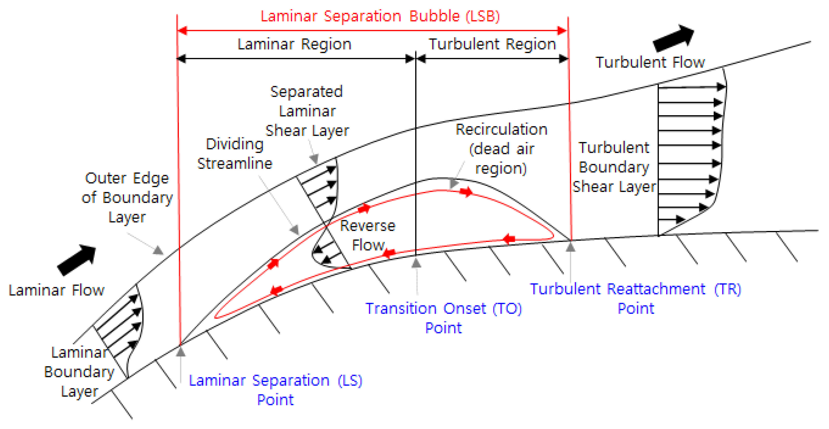
The general flow structure of an LSB and a separation-induced transition on an airfoil are illustrated in Figure 1. It shows that the LSB is composed of two regions: laminar (LS point to TO point) and turbulent (TO point to TR point) regions. The LSB is formed through the following processes; laminar boundary layer separation, transition to turbulence, and reattachment. When a laminar boundary layer separates at the LS point due to a strong adverse pressure gradient, the shear layer reattaches at the turbulent reattachment (TR) point, forming an LSB. The length between the LS point and the TR point is defined as the LSB that depends on the transition process in the shear layer. The length and location of the separation bubble strongly depend on the airfoil profile, free-stream turbulence intensity, free-stream Reynolds number, and the angle of attack [9,10]. Separation bubbles can be either short or long. According to the Tani [9], short bubbles reattach shortly after separation and therefore only have a local effect on the pressure distribution. In contrast, long bubbles completely change the pressure distribution creating a pressure plateau and hence produce large aerodynamic losses.
In general, there are three types of transitions; natural, bypass, and separation-induced transition. Out of these, the most prevalent type of transition observed for airfoils at low Reynolds numbers is the separation-induced transition, where a laminar boundary layer separates under the influence of a pressure gradient on airfoil surface [11,12]. As a result, a transition develops within the separated shear layer, which may reattach due to the enhanced mixing caused by the turbulent flow. This reattachment then forms an LSB at some distance downstream from the surface [13,14]. According to Mayle [15], a free-stream turbulence level of 1% is a boundary between natural and bypass transition with and without downstream development region of instability waves and thus a higher turbulence intensity (TI) than 1% can cause a shorter LSB. Furthermore, Choudry et al. [16], numerically confirmed that the increase of TI at a NACA 0021 airfoil triggers a delay in LS, resulting in a larger laminar zone and decrease of separation bubble length (SBL).
Understanding the characteristics of an LSB on an airfoil has been the subject of many investigations, both experimentally and numerically, over the last few decades [6,10,17], but the overall LSB dynamics are still not completely understood. The experimental approaches to LSBs have been discussed to understand the complex nature of this phenomenon. A combination of hot-wire anemometry, high-speed flow visualization, and velocity and surface pressure measurements was also used to study LSB dynamics on a NACA 0018 airfoil, with an emphasis on the formation of roll-up vortex, evolution, and detachment [18]. However, experimental approaches to the measurement of LS and transition onset (TO) points are both expensive and time consuming. Thus, as an alternative, computational fluid dynamics (CFD) approaches which use numerical modeling techniques, are more preferred for the accurate prediction of the aerodynamic performance of airfoils [19,20,21]. However, one of the major challenges in the accurate simulation of airfoil aerodynamics is to reproduce the transitional flow. In this regard, predicting the transition from laminar to turbulent flow is extremely crucial, especially when LSBs are present around the airfoil at high AoAs.
To the authors’ best knowledge, very few publications about characteristics and effects of the LSBs on the S809 airfoil are available in the literature, despite its importance regarding aerodynamic performance. A number of studies have used two equation turbulence models to acquire comparatively fast results, whereas direct methods of direct numerical simulation (DNS) and large eddy simulation (LES) are prohibitively expensive for industrial applications [22,23]. To further avoid the difficulties of the methods, recently, approaches based on the Reynolds-averaged Navier–Stokes (RANS) equations coupled with linear stability theory have been suggested as an attractive alternative for accurate prediction of the separation-induced transition. Pasquale et al. [24] extensively reviewed transition models for CFD and Menter et al. [11,12,25] suggested a new transition model called -, which can be readily implemented into an existing RANS solver.
Therefore, the objective of this study is to achieve a better understanding of the LSB characteristics on pressure and suction airfoil surfaces to prevent the unintended degradation of airfoil performance and accurately predict the aerodynamic coefficients of an airfoil. Detailed analysis was performed to investigate the characteristics of the LSB and its subsequent effects on the aerodynamic performance of the NREL S809 airfoil as a function of AoA. A numerical approach utilizing the - transition model, first proposed by Menter et al. [25], was adopted using commercial CFD software (ANSYS FLUENT 19.4 solver, Ansys, Canonsburg, PA, USA). The simulation results were compared and validated with the aerodynamic properties of the wind turbine airfoil experimentally obtained at the Delft University 1.8 m × 1.25 m low-turbulence wind tunnel [26]. The following properties were studied as a function of AoA: the flow structure of the LSB, the TO point at the onset of turbulence, the reattachment point on the pressure and suction airfoil surfaces, and the relationship between the extent of the separation bubble and the lift-to-drag ratio.
2. Transition Modeling
2.1. Transport Equations for the Transition SST Model
The transition shear stress transport (SST) model, known as the - model, is used in this study. This model is based on coupling of the SST - transport equations with two other transport equations for the intermittency, and for the transition momentum thickness Reynolds number (). The intermittency equation is used to control the production of turbulent kinetic energy in the boundary layer. The TO Reynolds number transport equation is developed in order to avoid the additional non-local operations introduced by quantities used in the experimental correlations. These correlations are typically based on the TI or the pressure gradient outside the boundary layer. This model is able to provide an accurate prediction of the TO point as it allows the intermittency to vary across the boundary layer. Instead of using the momentum-thickness Reynolds number, the - model is based on the vorticity Reynolds number [25], which is dependent solely on local variables, as:
where, Ω is the vorticity (shear strain rate) and is the wall normal distance. The maximum value of is dependent on the momentum thickness Reynolds number as follows:
The transport equation for the intermittency is formulated to trigger the transition process and is given by [25]:
where the transition sources, and are defined as follows:
where, S is the strain rate magnitude, is an empirical correlation that controls the length of the transition region, and and have constant values of 2 and 1, respectively.
and in Equation (3) represent the destruction and relaminarization sources defined as:
The transport equation for the transition momentum thickness Reynolds number is defined as follows:
Outside the boundary layer, the source term is employed to force the transported scalar to match the local value of calculated from an empirical correlation. The source term is defined as
The studied fan where is a time scale and the blending function is used to turn off the source term in the boundary layer and allow the transported scalar to diffuse in from the freestream. In the free stream, is 0, and in the boundary layer it equals 1.
2.2. Separation-Induced Transition Correlation
It is known that when a laminar boundary layer separation occurs, the present transition model consistently predicts the TR location too far downstream [11]. This is because the turbulent kinetic energy (k) in the separating shear layer is smaller at lower free-stream turbulence intensities. Therefore, a modification for the separation-induced transition is applied by the following equation:
where, is a constant with a value of 2. The model constants in this equation have been adjusted from those by Menter et al. [11] in order to improve the predictions of the separated flow transition. The main difference is that the constant that controls the relation between and was changed from 2.193 for a Blasius boundary layer to 3.235 at a separation point where the shape factor is 3.5 [11]. The transition model has been coupled with Menter’s - SST turbulence model [15], in which the production and destruction terms from the turbulent kinetic energy equation in the original SST model have been modified using the intermittency. In order to capture the laminar and transitional boundary layers correctly, the mesh should have a of approximately one.
2.3. Coupling the Transition Model and SST Transport Equations
The transition model interacts with the SST turbulence model by modification of the -equation, as follows:
where, and are the original production and destruction terms for the SST model. Note that the production term in the ω-equation is not modified. The reason behind the above model formulation is given in detail in [11]. A complete description of the model is available in [11,12]; the full model is quite large and is not repeated here in the interest of space.
3. Numerical Simulation
3.1. Governing Equation
The flow governing equations are solved using a cell-centered control volume space discretization approach for the fluid domain. The continuity equation and RANS equation can be expressed in Cartesian tensor form as follows:
The Reynolds term ( is an additional term that represents the effects of turbulence and must be modeled in order to close the RANS equation. A common method employs the Boussinesq hypothesis to relate the Reynolds stress to the mean velocity gradients as follows:
Here, the turbulent viscosity, , is computed by combing and (explained earlier in Section 2.3) as
where, the coefficient damps the turbulent viscosity causing a low-Reynolds number correction.
3.2. S809 Airfoil Specifications
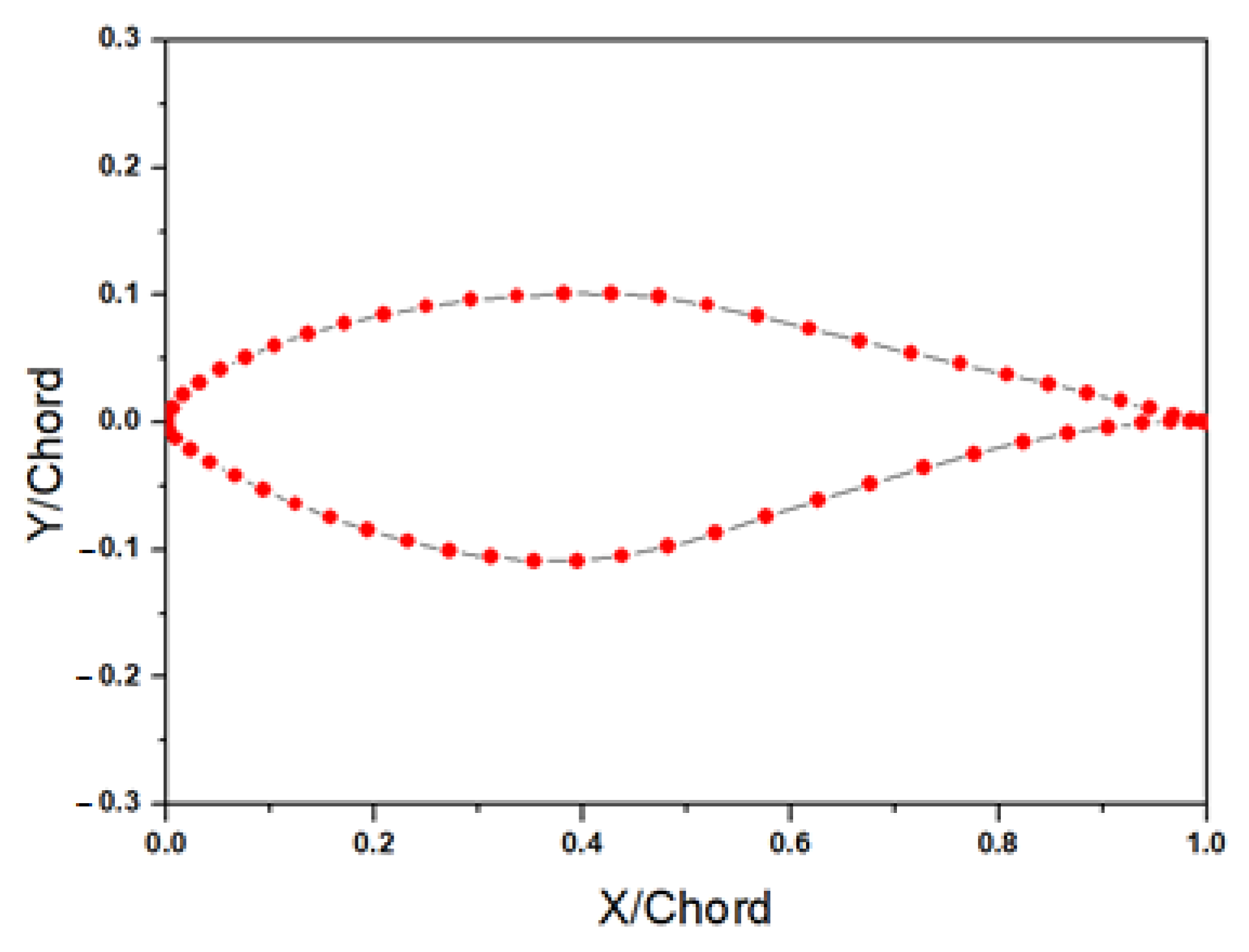
The wind turbine airfoil model considered in this study is S809 airfoil designed by the National Renewable Energy Laboratory (NREL) for phase VI small wind turbine blade. The S809 is a laminar-flow airfoil with 21% thickness, as shown in Figure 2. It was specifically designed and analyzed theoretically using the Eppler design program developed by Eppler and Sommers [27,28] for maximum sustained lift, insensitivity to surface roughness, and low profile drag. The airfoil model was tested in the low-turbulence wind tunnel of the Delft University of Technology Low Speed Laboratory in The Netherlands [26], which the numerical results of the present study will be compared with for validation of the model. The geometry of the airfoil is also adopted from [26,29]. For a higher resolution, interpolations of the upper and lower side profiles of the airfoil using a cubic spline curve, as shown in Figure 2, were used in this study.
3.3. Computational Mesh
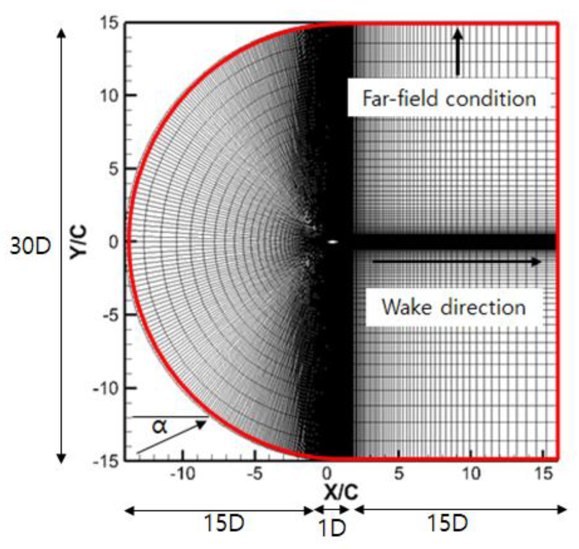
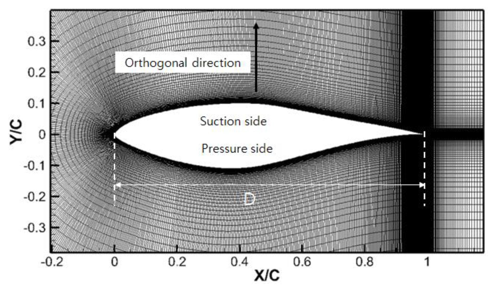
In this study, ANSYS Workbench was used to generate turbulent flow simulations around the S809 airfoil with two kinds of turbulence models (standard - and - transition models). The mesh employed for the simulations is illustrated in Figure 3 and Figure 4. The computational domain has a C-type grid topology, which consists of a normal distance of 150 m (15D) and a wake direction of 160 m (16D) from the leading edge. The airfoil was placed approximately in the middle of the computational boundary at a distance of 15 chord lengths from the half circle boundary in order to ensure that the boundary location did not influence the flow. A total of 69,000 elements were used to model the flow, with 246 grid points along the airfoil upper and lower surface each, 100 in the orthogonal direction, and 100 in the wake direction. A total of 25 inflation layers with the expansion ratio of 1.1 in the normal direction were applied in order to accurately capture the boundary layer region and the height of the first layer was 0.005 mm. The transition model was set for a maximum of 1 needed for the high-Re turbulent models. For values between 0.001 and 1, there is almost no effect on the solution [26]. In addition, for the comparison with the standard - turbulence model proposed by Launder and Spalding [30], the additional grid with the standard wall function of 30~100 was used, which is based on a semi-empirical formula to bridge the viscosity-affected region between the wall and the fully turbulent region. The lower limit should always be in the order of ~15. Wall functions typically deteriorate below this limit, and the accuracy of the solutions cannot be maintained [31].
3.4. Analysis Conditions and Far-Field Boundary Condition
The study was conducted using ANSYS FLUENT 19.4, which is a general-purpose commercial CFD code based on a cell-centered finite-volume method. There are several types of solver algorithms available in FLUENT, including coupled explicit, coupled implicit and segregated solvers. For the computations presented in this paper, we selected the segregated solver to speed up the convergence. The pressure-velocity coupling was obtained through the SIMPLE algorithm, and a green-gauss cell-based scheme was used for the gradient spatial discretization. Second-order upwind schemes were employed for pressure, momentum, and turbulence equations. The steady state computation was performed for approximately 20,000 iterations where the convergence tolerance for all relevant variables was less than 0.001% and changed from a default value of 0.1% due to the experimental data with five decimal places. Note that the results were taken using the average of the last 2000 datapoints acquired at each iteration step due to the oscillation problem for each variable occurring in the convergence history. However, the occurrence of the oscillation phenomenon, which means unsteady physical flow characteristics, is general and natural in the wall-bounded transitional flows with separation bubbles when the convergence criterion becomes very low. Therefore, averaging the last data is a reasonable method to accurately predict aerodynamic coefficients.
The analysis was carried out at a low Reynolds number of 2.0 × 10⁶ for the angles of 0°, 1.02°, 5.13°, 6.04°, 8.04°, 9.22°, 14.24°, and 20.15°. The Reynolds number corresponds to Mach number of 0.04797 converted to velocity of 16.31 m/s. A TI of 0.03% was applied from the experimental results as the turbulence level in the test section of NREL wind tunnel varied from 0.02% at 10 m/s to 0.04% at 60 m/s [26]. The free-stream turbulent kinetic energy and the specific dissipation rate of turbulent energy were 3.59 × 10⁻⁵ m2/s2 and 0.44 1/s, respectively. This is based on TI of 0.03% and density () of 1.226 kg/m3 using Equations (21) and (22), where is an empirical constant specified in the turbulence model and is the turbulent viscosity ratio.
A pressure far-field condition for all the boundaries except for the airfoil was used to model a free-stream condition at infinity, with a free-stream Mach number. The pressure far-field boundary condition is often called a characteristic boundary condition, since it uses characteristic information to determine the flow variables at the boundaries. This boundary condition is applicable only when the density is calculated using ideal-gas law.
3.5. Grid Independence Study
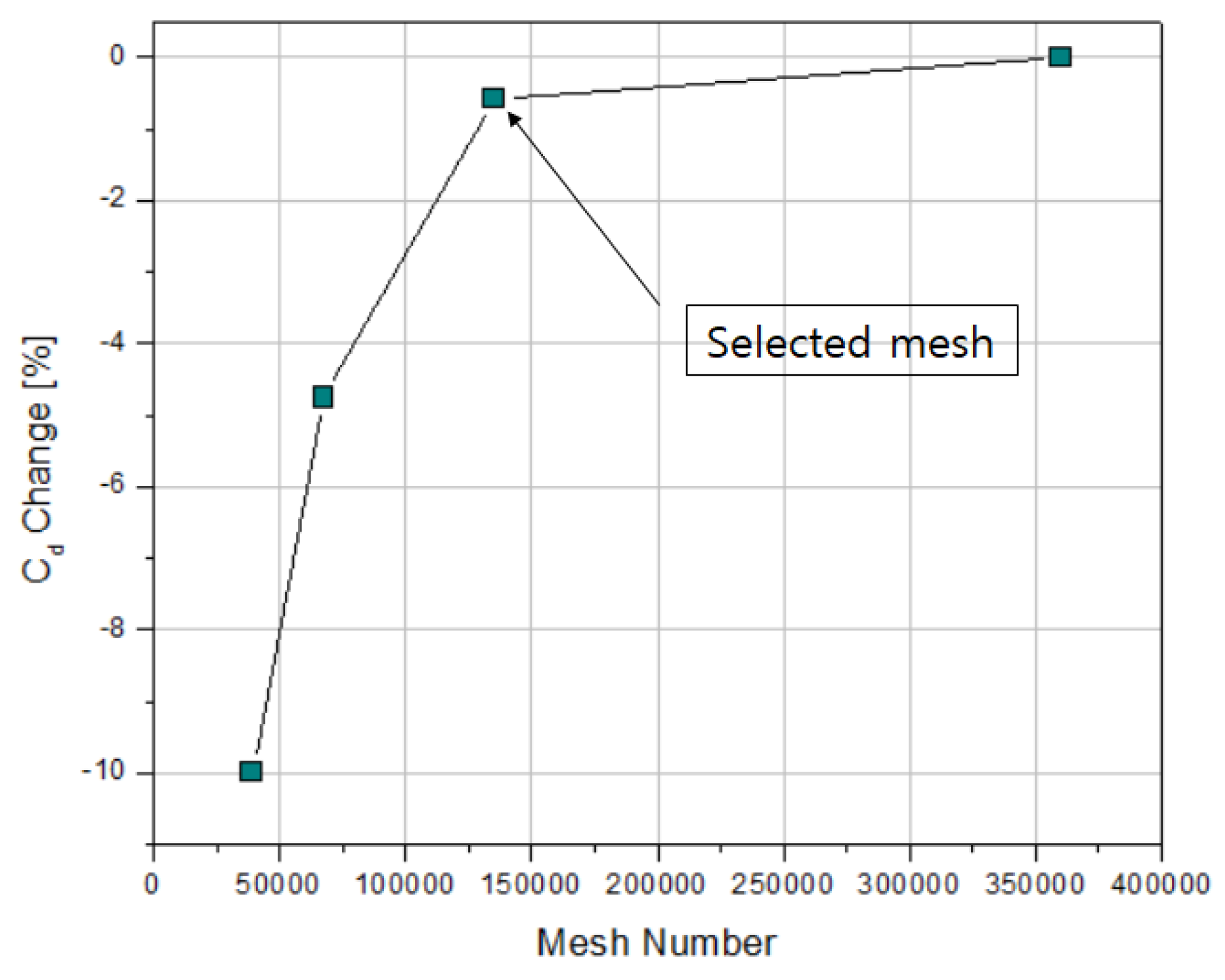
Mesh grid size is an important factor in numerical simulations because resolving the transitional flow depends significantly on the grid size to accurately describe the flow. Thus, a grid independence study at AoA = 0° was conducted to ascertain whether the selected grid density had sufficient resolution and to confirm that the spatial discretization errors were minimal. Moreover, the low AoA of 0° can achieve a better convergence than higher AoAs, and thus, only the grid size effect can be observed at the same condition. Table 1 shows the properties of four grids that were generated. The number of grid elements of Grid 2 in the lower and upper sides of the airfoil and the wake direction was doubled for Grid 1, and was halved for Grid 3. Grid 4 was the finest grid generated using 360,000 grid elements. Figure 5 depicts a representative example of the change in Cd (percent) as a function of the mesh number for the S809 airfoil. This serves to identify a mesh resolution that provides a reasonable tradeoff between accuracy and computational burden. By further increasing the number of grid elements, it is confirmed that using Grid 3 results in a value (−0.58%) that is within the acceptable range of variation compared to Grid 4. This indicates that we have reached a solution that is independent of the mesh resolution. By considering the computation time and the minimal variation in the drag coefficient between the four cases, Grid 3 was found to be optimal in terms of accuracy and computation time. Therefore, the transition and standard - turbulence models for Grid 3 were applied with the same elements by differently adjusting the distance of the first grid from the airfoil for the value requirements of each model, as already described in Section 3.3. To the best of the authors’ knowledge, compared to other S809 airfoil simulation results in the literature, the present simulation results for the airfoil aerodynamic performance can be regarded as highly accurate.
4. Results and Discussion
4.1. Validation of the Simulation
4.1.1. Comparison of Pressure Coefficients
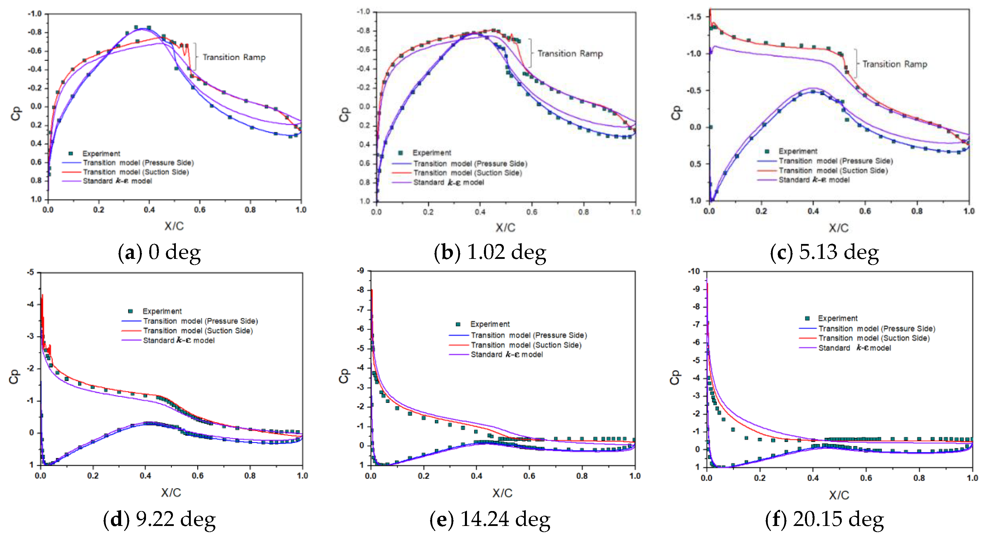
In order to validate the numerical model, the results were compared with experimental data. Due to the effect of AoA on the transition location, the validation was done for a range of AoAs for which experimental data were available. The computed pressure coefficient (Cp) distributions along the blade chord at different AoAs of 0°, 1.02°, 5.13°, 9.22°, 14.24°, and 20.15° for a Reynolds number of 2.0 × 10⁶ are compared with the experimentally measured values in Figure 6 [26,29]. The blade chord presented is expressed as a normalized distance of X/C. The computed pressure coefficients calculated from the transition model show a very good agreement with the pressure measurements on the suction and pressure sides for all the angles. On the other hand, the simulation results of the standard - turbulence model were overpredicted or underpredicted over the blade chord for the all the angles due to a delay in LS. It is noteworthy that small discrepancies between the pressure coefficients by the transition simulation exist near the suction side below X/C = 0.5 and over X/C = 0.8 for the high angle of 14.24°. These discrepancies might be due to a stall by the vortex shedding and a strong vertical disturbance over the suction surface, occurring near a stall angle of 16° [32]. Similarly, discrepancies can be observed near the suction side for the high angle of 20.15°. Nonetheless, these discrepancies are of such small magnitude that they are unlikely to affect the flow field caused by LSBs on the airfoil. The transition ramp, which is defined as the region over which the bubble moves with increasing AoA, was found on the suction side, as can be clearly seen in Figure 6a–c [26,29]. It is interesting to note that as the AoA is increased, the TO point moves forward as the suction side pressure gradient becomes more adverse. Since the flow field characteristics around an airfoil are closely related to the change in axial and angular momentum [33] that leads to the pressure distribution on the airfoil, accurate predictions of the pressure coefficients along the airfoil provide the necessary validation for the subsequent LSB analysis.
4.1.2. Comparison of Aerodynamic Coefficients
Table 2 and Table 3 present the comparison of the simulation results from the transition model and the standard - model for the drag and lift coefficients at the six AoAs and the experimental results [26,29]. The numerical lift and drag coefficients calculated from mixed laminar/turbulent flows obtained with the semi-transition model by [29] are also presented. The transition calculations in the present study show a very good agreement with the measured data even at AoAs higher than 9.22°. The exceptions to this are the drag coefficients at 14.24° and 20.15°, which are underpredicted by 33% and 38%, respectively. This is primarily due to the sharp truncated trailing edge on the airfoil, where the drag is underpredicted [34]. Slight underpredictions for the drag coefficient of 8% and 9% are observed at 0° and 1.02°, whereas lift coefficient overpredictions between 7.3% and 21.1% are observed at AoAs higher than 9.22°. On the other hand, the simulation results by the standard - model are largely overpredicted or underpredicted in the range of 389% to 36%. Accordingly, the transition results show considerably better predictions than the standard - model. In addition, the transition simulations are found to be more accurate than the mixed laminar/turbulent flows obtained with the semi-transition model suggested in [29]. In particular, the semi-transition model was applied by splitting the computational region into laminar and turbulent domains and specifying laminar and turbulent zones using the standard - model in each domain. However, the accuracy of the semi-transition model depends strongly on the transition location. Owing to the known transition location from the experimental report [26,29], it is expected that the semi-transition model results provide a reasonable match with the experimental results. Therefore, the semi-transition model has a notable disadvantage in that the TO point from the experiment should be suggested in advance, prior to the simulation. Hence, this methodology is not currently useful for predicting the LS on an airfoil. Overall, comparison of the - transition model results with the experimental data demonstrated a good agreement. Accordingly, the subsequent LSB analysis is considered to be of sufficient accuracy.
4.2. Laminar Separation-Induced Transition
4.2.1. Laminar Separation-Induced Transition
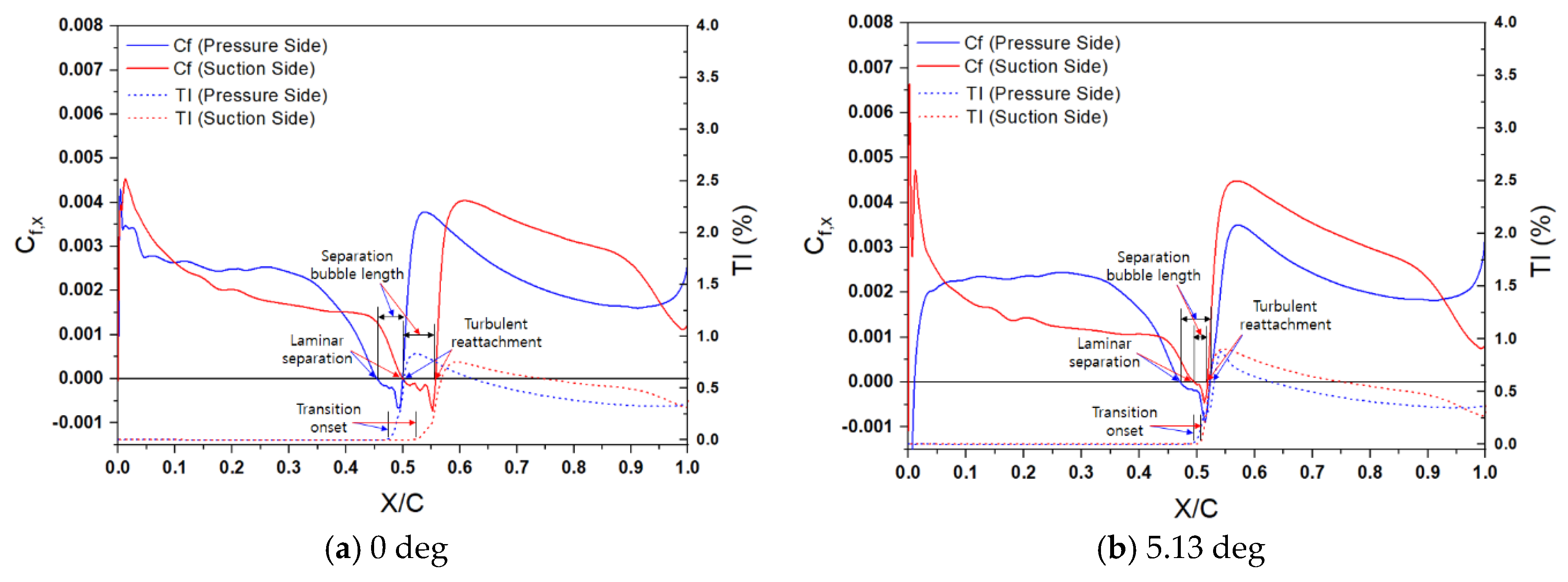
The skin friction coefficient ( and TI on the airfoil’s lower surface (pressure side) and upper surface (suction side) as a function of X/C are shown in Figure 7. The predictions from the - transition model are compared at two representative angles of 0° and 5.13°. The and TI curves for the pressure airfoil surface are shown as the blue lines, whereas those for the suction airfoil surface as the red line. The distributions on each surface clearly depicts the points of LS, TO, TR, and SBL. Figure 7a,b indicate that at an AoA of 0°, the laminar boundary layers on the pressure and suction airfoil surfaces separate at X/C = 0.455 and 0.50, respectively. In addition, the shear layers reattach at X/C = 0.499 and 0.557, respectively. This results in SBLs of 4.44% and 5.74% the chord length, respectively. As the AoA is increased to 5.13°, the LS on the pressure and suction airfoil surfaces is generated at X/C = 0.471 and 0.496 and is reattached at X/C = 0.523 and 0.518, resulting in SBLs of 5.17% and 2.24% the chord length, respectively. Therefore, as the AoA is increased, the bubble on the suction surface moves closer to the leading edge due to an earlier LS caused by the increased adverse pressure gradients, whereas the bubble on the pressure surface moves downstream due to a later LS. In addition, for Re = 2.0 × 10⁶, the bubble on the pressure side is longer by 0.73% (5.17% − 4.44%) of the chord length (compared to an AoA of 0°), whereas on the suction side the bubble is shorter by 3.5% (5.74% − 2.24%) of the chord length (than for an AoA of 0°). Similar observations were made in the experiments by [26].
TO in this study is defined as the location where the TI just starts to increase after the separation. Using this definition, it can be observed that at the AoA of 0°, a TI of 0.03% at the far-field condition suddenly increases on the pressure and suction airfoil surfaces at the TO points of X/C = 0.476 and 0.526. This is observed to occur after the LS points at X/C = 0.455 and 0.50, and after the TR points at X/C = 0.523 and 0.518 reach maximum values of 0.83% and 0.75% at X/C = 0.524 and 0.592, respectively (Figure 7a). Similarly, as the AoA is increased to 5.13°, the TI starts to increase at the TO points of X/C = 0.495 and 0.508 after the LS points of X/C = 0.471 and 0.496, and after the TR points of X/C = 0.523 and 0.518 reach maximum values of 0.88% and 0.91% at X/C = 0.543 and 0.547 on the pressure and suction airfoil surfaces, respectively (Figure 7b). Hence, with increase in AOA the TO on the suction side moves closer to the leading edge and moves downstream on the pressure side since the separation occurs at a smaller and larger distance to the leading edge, respectively.
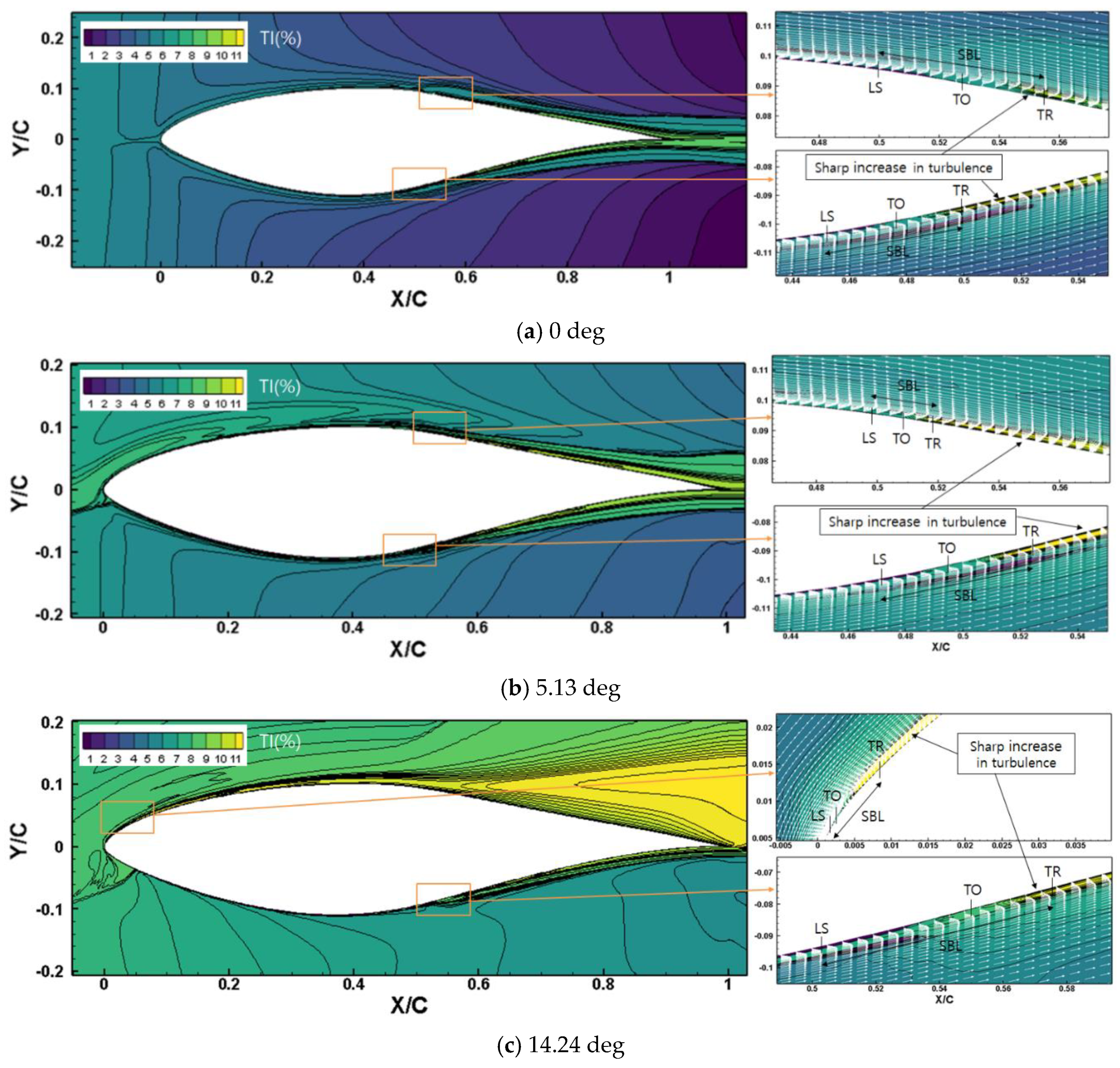
The distribution of TI and the overlapped distribution of the velocity vector and TI at AoAs of 0°, 5.13°, and 14.4° and close-up views of the LSB on the S809 airfoil are shown in Figure 8. The points of LS, TR, TO, and SBL are also shown. The shift of the LS point closer to the leading edge and trailing edge on the suction and pressure surfaces by increasing AoA can be seen in Figure 8. The Figure 8 shows that at the AoA of 0°, the separated shear layer reattaches on the upper (suction) surface around the mid-chord length and on the lower (pressure) surface just forward of the mid-chord length, resulting in the formation of different sizes of separation bubbles on each surface. This is primarily due to the increased adverse pressure along each surface gradient prior to the onset of turbulence, as stated earlier. As the AoA increases, the adverse pressure gradient on the suction surface increases near the leading edge of the airfoil, leading to earlier separation of the laminar boundary layer and consequently the increased turbulence level up to a maximum of 30%. From a close-up view at the AoA of 14.24°, earlier TO and TR are triggered upstream. Therefore, the SBL on the suction surface decreases as the bubble moves upstream with increasing AoA.
4.2.2. Effects of the Separation Bubble
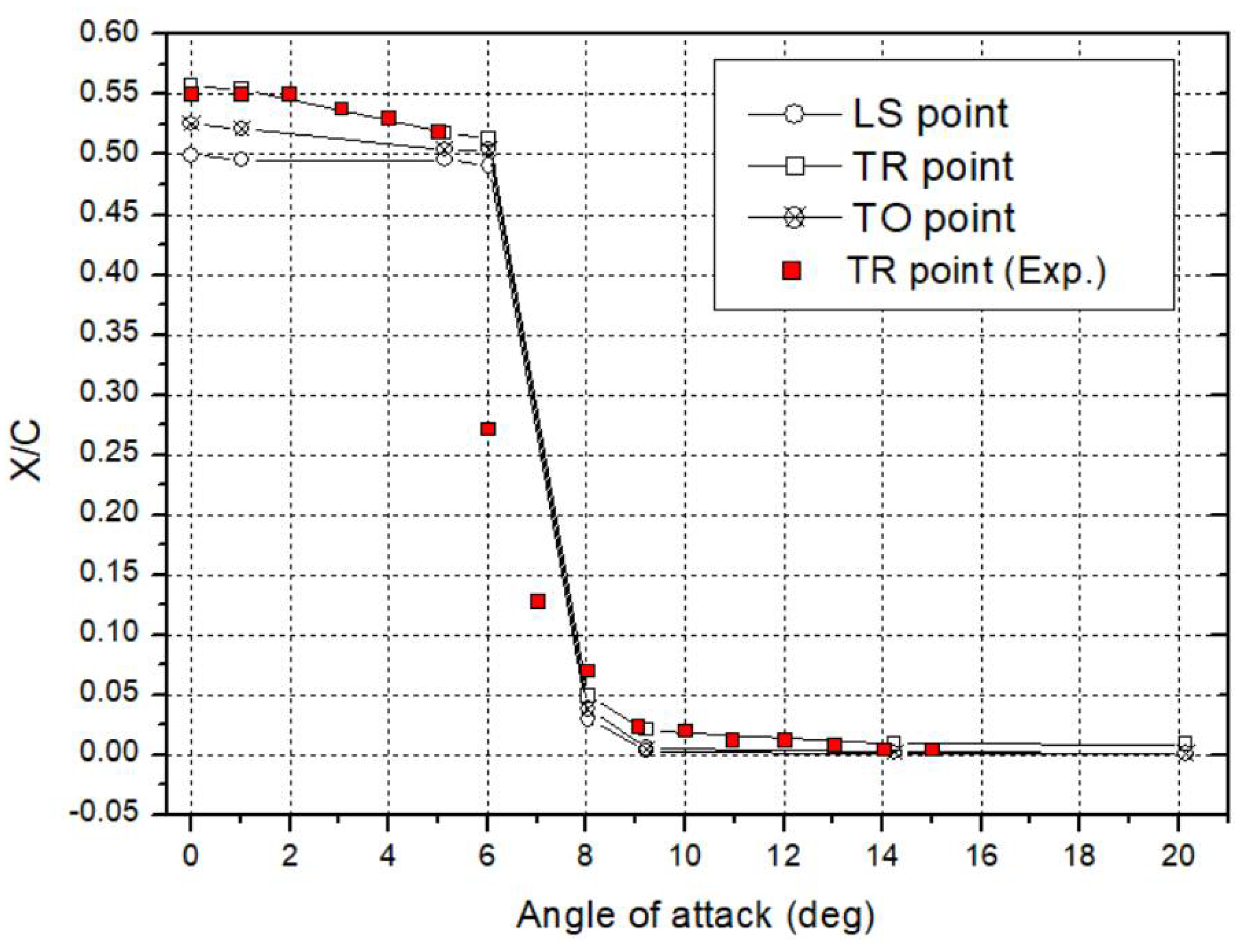
The LS, TR, and TO points on the suction airfoil surface for each AoA are plotted in Figure 9. The TR points overall show a very good agreement with the experiments between AoAs of 0° and 15°, except those between 6.03° and 8.04°, between which a sudden jump of the separation point to the upstream occurred because the transition model approaches could represent regions at which the LSB changed. The simulations showed that the transition model was not able to detect the unsteady characteristics of the flow for AoAs between 6.03° to 8.04°, which will be further studied in future using large eddy simulation. It must also be noted that the TO points indicating the turbulence onset could not be compared to the experiment by Van Ingen et al. and Somers as it was not reported in [26]. According to Figure 9, as the AoA increases from 0° to 5.13°, the transition location moves from 0.523 to 0.504 X/C, which shows that the minor effect of small AoAs on the transition location of the suction side. At the AoA of 9.22°, which is smaller than the 2D stall angle of 16°, the separation bubble on the upper surface jumps to the leading edge of the airfoil [32]. When the AoA is greater than 9.22°, the transition always occurs at the leading edge.
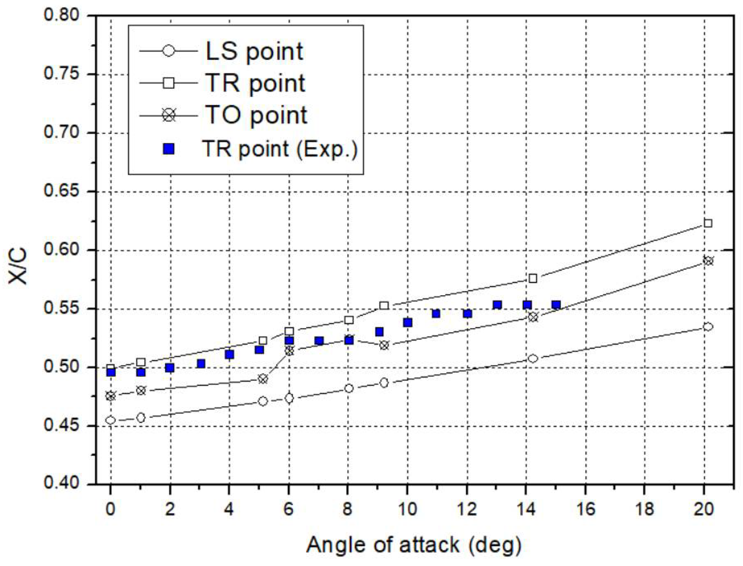
The LS, TR, and TO points on the pressure side of the airfoil for each AoA are plotted in Figure 10. The TR points show a good agreement with the experiments, except for small deviations at higher AoAs. With increasing AoA from 0° to 20.15°, the TO point moves downstream from 0.476 to 0.591 X/C without abrupt jumps along the surface. This shows that increasing the AoA gives rise delays separation on the pressure side with the weak adverse pressure gradient.
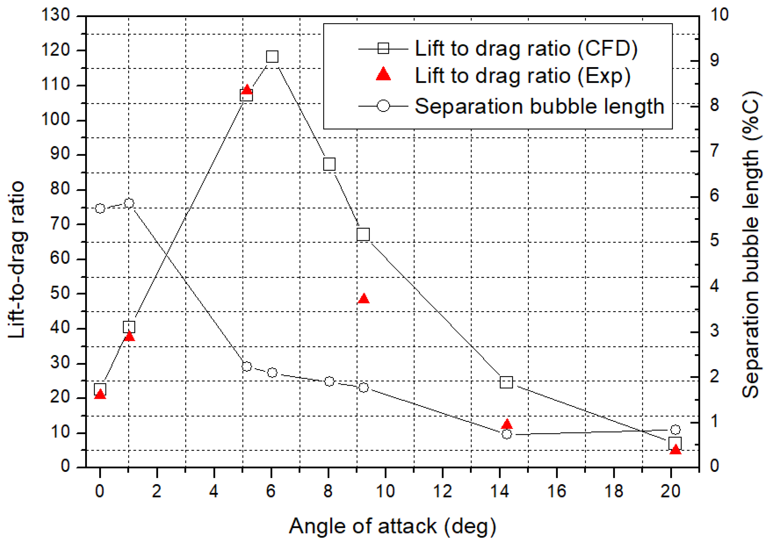
The SBL on the suction airfoil surface and the airfoil lift-to-drag ratio (Cl/Cd) are presented in Figure 11. As the AoA increases, the extent of the LSB decreases from 5.74% of the chord length at 0° to 0.841% the chord length at 20.15°, except for a little increase to 5.86% the chord length at 1.02°. The change in the size occurs primarily because of upstream movement of the TR point due to a strong adverse pressure gradient in the separated shear layer. According to Bastedo and Mueller [31], a separation bubble with a size of less than a maximum of 5.86% the chord length can be classified as a short separation bubble. The simulation results also show that the lift-to-drag ratios obtained by using the transition model are 104.1 and 118.4 at the AoAs of 5.13° and 6.03°, respectively, when the corresponding bubble sizes are 2.24% and 2.11% of the chord length, whereas the Cl/Cd value obtained by using the standard - model (Table 2 and Table 3) is 17.2 at the AoA of 5.13°. A maximum Cl/Cd ratio at a designed AoA is an important factor in accurately predicting and maximizing the power of wind turbine blade, based on the BEM theory [7]. The results of the transition and standard - models showed the Cl/Cd ratio underpredictions of 4.2% and 84.1%, respectively, at AoA of 5.13° when compared to the experimental value of 108.7, whereas the Cl/Cd ratio of the semi-transition model was 109, which showed overprediction of 0.3%. However, the semi-transition model approach is not currently useful for predicting the transition location because the experiments should be suggested in advance, prior to the simulation, as described in the previous section. Therefore, the Cl/Cd ratio values of the transition and standard - models cause deviations of 0.17% and 25.4% in power, respectively, based on the BEM theory-based calculations [7], when rotational speed, local chord length, and local radius are 71.9 rpm, 0.59 m, and 2.71 m, respectively; the local twist angle, rotor radius, and tip speed ratio are 2.754°, 5.029 m, and 2.915, respectively; and the local solidity, wind speed, density, and span length for the blade element are 0.0693, 7 m/s, 1.246 kg/m3, and 0.59 m, respectively. A complete description of the BEM theory-based calculations has been reported elsewhere [7] because explaining in greater detail is out of the scope of this research. The bubble lengths at AoAs of 8.04°, 9.22°, 14.24°, and 20.15° are 1.92%, 1.78%, 0.74%, and 0.84% of the chord length, respectively. According to Choudry et al. [16], a decrease in the bubble extent of 9% causes an improvement in the maximum lift-to-drag ratio of approximately 17%. Therefore, the aerodynamic performance of the airfoil can be considerably improved by the mitigation of the bubble by increasing the laminar region, thus decreasing the drag, and enhancing lift-to-drag ratio due to a smaller bubble size.
5. Conclusions
Numerical simulations using the - transition model coupled with SST - transport equations around the 21% thick NREL S809 airfoil were performed to achieve a better understanding of the characteristics and effects of LSBs existing at a low Reynolds number and low TI. The computational domain had a C-type grid topology with a pressure far-field condition, and the analysis was carried out under various AoAs. The reliability and validity of the simulations were verified using published results of experiments. The transition model case showed very good agreement with the experimental case in terms of aerodynamic lift and drag coefficients, and characteristics of LSBs owing to the higher predictive accuracy relative to the standard - model case. These comparisons provide sufficient evidence that the predictions of the LSB are accurate, as evidenced by the fact that the aerodynamic characteristics of the airfoil are closely related to the characteristics of the LSB. Consequently, the transition model-based approaches, which have a high predictive accuracy, presented herein can elucidate the characteristics and effects of the LSB on airfoil aerodynamic performance. Important findings arising from this research are as follows:
The transition ramp, which is defined as the region over which the LSB moves with increasing AoA, was clearly observed on the suction airfoil surface. It was confirmed that the TO point on the suction side of the S809 airfoil moved upstream due to an earlier LS caused by increased adverse pressure gradients as the AoA increased. Therefore, the accurate predictions of the pressure coefficients along the airfoil using the transition model offered the necessary validation for the subsequent LSB analysis.
At the AoA of 0°, the location of the LSB on the pressure and suction airfoil surfaces was observed to be generated at X/C = 0.455 and 0.50 and to be reattached at X/C = 0.499 and 0.557, causing SBLs of 4.44% and 5.74% the chord length, respectively, between LS and TR. Furthermore, when the AoA increased to 5.13°, the location of the LSB moved to X/C = 0.471 downstream and to X/C = 0.496 upstream, resulting in an SBL that is taller by 0.73% the chord length and shorter by 3.5% the cord length for the pressure and suction airfoil surfaces, respectively. Therefore, the suction surface prediction featured a slightly earlier LS compared to the pressure surface.
It was observed that the TI increased suddenly on the pressure and suction airfoil surfaces at the TO points of X/C = 0.476 and 0.526 after the LS points at X/C = 0.455 and 0.50, respectively, at the AoA of 0°. At the AoA of 5.13°, this increase occurred at X/C = 0.495 and 0.508 after the LS points of X/C = 0.471 and 0.496, respectively, which caused the production of turbulent kinetic energy in the separated laminar shear layer. Moreover, at the AoA of 0°, the TI reached maximum values of 0.83% and 0.75% at X/C = 0.524 and 0.592 after the TR points of X/C = 0.523 and 0.518, respectively. At the AoA of 5.13°, the TI reached maximum values of 0.88% and 0.91% at X/C = 0.543 and 0.547 after the TR points of X/C = 0.523 and 0.518, respectively. Therefore, the simulation results demonstrated a sharp increase in turbulence levels during the transition process, immediately after the LS, and a maximum TI value after the TR.
The separation bubble on the suction surface jumped to leading edge of the airfoil at the AoA of 9.22°, whereas on the pressure surface, it moved downstream. In addition, the maximum SBL was 5.86% the chord length at the AoA of 1.02°. The extent of the separation bubble slightly decreased to 0.841% the chord length at 20.15°. Therefore, an SBL of less than a maximum of 5.86% the chord length on the S809 airfoil can be identified as a short separation bubble.
The Cl/Cd ratios of the transition and standard - models at the AoA of 5.13 were 104.1 and 17.2, respectively, which shows underpredictions of 4.2% and 84.1% with respect to the experimental value of 108.7, whereas the Cl/Cd ratio of the semi-transition model was 109, which showed overprediction of 0.3%. However, the direct comparison of the maximum lift-to-drag ratios with the semi-transition model was not presented because the model cannot currently predict the TO point without prior knowledge of the experimental results. Therefore, BEM theory-based calculations using these results of the transition and Standard - models led to deviations of 0.17% and 25.4%, respectively, in power.
Thus, an airfoil design with a high lift-to-drag ratio, and a high predictive accuracy of aerodynamic coefficients in simulation is required to maximize and accurately predict the performance of wind turbine blades, respectively, through a deep understanding of the characteristics and effects of the LSB on airfoil and the transition model approaches presented in the current study. The results of this study can help in redesigning an airfoil with a reduced bubble length causing the improved aerodynamic performance, and designing wind turbine blades that offer maximum power. Further investigations into the aerodynamic corrections for two-dimensional airfoil characteristic data and its effect will be conducted to improve the performance prediction of the wind turbine blades.
Author Contributions
J.-o.M. provided the basic idea for this study and the overall numerical strategies, and carried out the numerical simulations and worked on the analysis of numerical results. B.-s.R. supported the results and conclusion for this study. All authors have read and agreed to the published version of the manuscript.
Funding
This research received no external funding.
Acknowledgments
The authors would like to acknowledge the assistance of Maziar Arjomandi and student Azadeh Jafari at the School of Mechanical Engineering of the University of Adelaide in Australia.
Conflicts of Interest
The authors declare no conflict of interest.
References
- Pires, O.; Munduate, X.; Ceyhan, O.; Jacobs, M.; Snel, H. Analysis of high Reynolds numbers effects on a wind turbine airfoil using 2D wind tunnel test data. J. Phys. Conf. Ser. 2016, 753, 022047. [Google Scholar] [CrossRef]
- Meyers, J.F.; Dagenhart, J.R.; Harvey, W.D. A study of laminar separation bubble in the concave region of an airfoil using laser velocimetry. In Symposium on Laser Anemometry ASME, Proceedings of the 1985 Winter Annual Meeting, Miami, FL, USA, 17 November 1985; NASA Langley Research Center: Hampton, VA, USA, 1985. [Google Scholar]
- Lissaman, P.B.S. Low Reynolds number airfoil. Annu. Rev. Fluid Mech. 1983, 15, 223–239. [Google Scholar] [CrossRef]
- Almutairi, J.H.; Jones, L.E.; Sandham, N.D. Intermittent bursting of a laminar separation bubble on an airfoil. AIAA J. 2010, 48, 414–426. [Google Scholar] [CrossRef]
- Zhang, W.; Hain, R.; Kähler, C.J. Scanning PIV investigation of the laminar separation bubble on a SD7003 airfoil. Exp. Fluids 2008, 45, 725–743. [Google Scholar] [CrossRef]
- Jahanmiri, M. Laminar Separation Bubble: Its Structure, Dynamics and Control; Research Report; Chalmers University of Technology: Gothenburg, Sweden, 2011. [Google Scholar]
- Kim, B.S.; Kim, W.J.; Lee, S.L.; Bae, S.Y.; Lee, Y.H. Developement and verification of a performance based optimal design software for wind turbine blades. Renew. Energy 2013, 54, 166–172. [Google Scholar] [CrossRef]
- Mahmuddin, M. Rotor blade performance analysis with blade element momentum theory. In Proceedings of the 8th International Conference on Applied Energy—ICAE2016, Beijing, China, 8–10 October 2016; pp. 1123–1129. [Google Scholar]
- Tani, I. Boundary-layer transition. Annu. Rev. Fluid Mech. 1968, 1, 169–196. [Google Scholar] [CrossRef]
- Swift, K.M. An Experimental Analysis of the Laminar Separation Bubble at Low Reynolds Numbers. Master’s Thesis, University of Tennessee, Knoxville, TN, USA, 2009. [Google Scholar]
- Menter, F.R.; Langtry, R.B.; Likki, S.R.; Suzen, Y.B.; Huang, P.G.; Volker, S. A Correlation-Based Transition Model Using Local Variables: Part I—Model Formulation. Available online: https://0-doi-org.brum.beds.ac.uk/10.1115/GT2004-53452 (accessed on 2 September 2020).
- Menter, F.R.; Langtry, R.B.; Volker, S. Transition modelling for general purpose CFD codes. Flow Turbul. Combust. 2006, 77, 277–303. [Google Scholar] [CrossRef]
- Alam, M.; Sandham, N.D. Direct numerical simulation of ‘short’ laminar separation bubbles with turbulent reattachment. J. Fluid Mech. 2000, 41010, 1–28. [Google Scholar] [CrossRef] [Green Version]
- Horton, H. Laminar Separation Bubbles in Two and Three Dimensional Incompressible Flows. Ph.D Thesis, Queen Mary University of London, London, UK, 1968. [Google Scholar]
- Mayle, R.E. The role of laminar-turbulent transiton in gas turbine engines. J. Turbomach. 1991, 113, 509–537. [Google Scholar] [CrossRef]
- Choudry, A.; Arjouandi, M.; Kelso, R. A study of long separation bubble on thick airfoil and its consequent effects. Int. J. Heat Fluid Flow 2015, 52, 84–96. [Google Scholar] [CrossRef]
- Hoefener, L.; Nitsche, W. Experimental investigations of controlled transition of a laminar separation bubble in an axisymmetric diffuser. Exp. Fluids 2008, 44, 89–103. [Google Scholar] [CrossRef]
- Kirk, T.M.; Yarusevych, S. Vortex shedding within laminar separation bubbles forming over an airfoil. Exp. Fluids 2017, 58. [Google Scholar] [CrossRef]
- Zhang, Y.; Zhou, Z.; Wang, K.; Li, X. Aerodynamic characteristics of different airfoils under varied turbulence intensities at low reynolds numbers. Appl. Sci. 2020, 10, 1706. [Google Scholar] [CrossRef] [Green Version]
- Guo, T.; Jin, J.; Lu, Z.; Zhou, D.; Wang, T. Aerodynamic sensitivity analysis for a wind turbine airfoil in an air-particle two-phase flow. Appl. Sci. 2019, 9, 3909. [Google Scholar] [CrossRef] [Green Version]
- Douvi, D.C.; Margaris, D.P.; Davaris, A.E. Aerodynamic performance of a NREL S809 airfoil in an air-sand particle two-phase flow. Computation 2017, 5, 13. [Google Scholar] [CrossRef]
- Zauner, M.; Tullio, N.D.; Sandham, N.D. Direct Numerical Simulations of Transonic Flow around an Airfoil at Moderate Reynolds Numbers. AIAAJ 2019, 57. [Google Scholar] [CrossRef]
- Asada, K.; Kawai, S. Large-eddy simulation of airfoil flow near stall condition at Reynolds number 2.1 × 10⁶. Phys. Fluids 2018, 30, 085103. [Google Scholar] [CrossRef]
- Pasquale, D.D.; Rona, A.; Garrett, S. A selective review of transition modelling for CFD. In Proceedings of the 39th AIAA Fluid Dynamics Conference, San Antonio, TX, USA, 22–25 June 2009; Available online: https://repairpal.com/radiator-fan-assembly (accessed on 15 June 2020).
- Menter, F.R.; Esch, T.; Kubacki, S. Transition modelling based on local variables. In Proceedings of the 5th International symposium on Engineering Turbulence Modelling and Measurements, Mallorca, Spain, 16–18 September 2002; pp. 555–564. [Google Scholar]
- Van Ingen, J.L.; Boermans, L.M.M.; Blom, J.J.H. Low-Speed airfoil section research at Delft University of Technology. In Proceedings of the 12th Congress of the International Council of the Aeronautical Sciences, Munich, Germany, 12–17 October 1980. [Google Scholar]
- Eppler, R.; Somers, D.M. A computer program for the design and analysis of low-speed airfoils. NASA 1980, 152, TM80210. [Google Scholar]
- Eppler, R.; Somers, D.M. Supplement to: A computer program for the design and analysis of low-speed airfoils. NASA 1980, 36, TM81862. [Google Scholar]
- Wolfe, W.P.; Ochs, S.S. CFD calculations of S809 aerodynamic characteristics. In Proceedings of the 35th Aerospace Sciences Meeting and Exhibit, AIAA. Reno, NV, USA, 6–9 January 1997. [Google Scholar]
- Launder, B.E.; Spalding, D.B. Lectures in Mathematical Models of Turbulence; Academic Press: London, UK, 1972. [Google Scholar]
- Bastedo, W.G.; Mueller, T.J. Spanwise variation of laminar separation bubbles on wings at low Reynolds number. J. Aircr. 1986, 23, 687–694. [Google Scholar] [CrossRef]
- Hand, M.M.; Simms, D.A.; Fingersh, L.J.; Jager, D.W.; Cotrell, J.R.; Schreck, S.; Larwood, S.M. Unsteady Aerodynamics Experiment Phase VI: Wind Tunnel Test Configurations and Available Data Campaigns; NREL/TP-500-29955; NREL: Golden, CO, USA, 2001. [Google Scholar]
- Burton, T.; Sharpe, D.; Jenkins, N.; Bossanyi, E. Wind Energy Handbook; John Wiley & Sons: Hoboken, NJ, USA, 2001. [Google Scholar]
- Baker, J.P.; Van Dam, C.P. Drag reduction of blunt trailing-edge airfoils. In Proceedings of the BBAA VI International Colloquium on Bluff Bodies Aerodynamics & Applications, Milano, Italy, 20–24 July 2008. [Google Scholar]
Figure 1.
General characteristics of a laminar separation bubble (LSB) and separation-induced transition, reproduced from Horton (1968).
Figure 1.
General characteristics of a laminar separation bubble (LSB) and separation-induced transition, reproduced from Horton (1968).

Figure 2.
S809 airfoil profile with a 21% thickness.

Figure 3.
C-type grid topology used in this study, showing the overall grid resolution and boundary conditions.
Figure 3.
C-type grid topology used in this study, showing the overall grid resolution and boundary conditions.

Figure 4.
Close-up view of the mesh in the vicinity of the airfoil.

Figure 5.
Cd percent change based on Cd = 0.006497 for the finest mesh (Grid 4) at each calculation as a function of mesh resolution for the NREL S809 airfoil with AoA = 0° and Re = 2 × 10⁶.
Figure 5.
Cd percent change based on Cd = 0.006497 for the finest mesh (Grid 4) at each calculation as a function of mesh resolution for the NREL S809 airfoil with AoA = 0° and Re = 2 × 10⁶.

Figure 6.
Comparison between the experiment and the simulation results of the pressure coefficient (Cp) with different turbulence models at selected angles of attack (AoAs) of 0° (a), 1.02° (b), 5.13° (c), 9.22° (d), 14.24° (e), and 20.15° (f) for the S809 airfoil (Re = 2 × 10⁶).
Figure 6.
Comparison between the experiment and the simulation results of the pressure coefficient (Cp) with different turbulence models at selected angles of attack (AoAs) of 0° (a), 1.02° (b), 5.13° (c), 9.22° (d), 14.24° (e), and 20.15° (f) for the S809 airfoil (Re = 2 × 10⁶).

Figure 7.
Comparison of x-direction skin friction coefficient ()
and turbulence intensity (TI) at the AoAs of 0° (a) and 5.13° (b) for both surfaces of the airfoil (pressure and suction sides).
Figure 7.
Comparison of x-direction skin friction coefficient ()
and turbulence intensity (TI) at the AoAs of 0° (a) and 5.13° (b) for both surfaces of the airfoil (pressure and suction sides).

Figure 8.
Distribution of TI and overlapped distributions of velocity vector and TI at selected AoAs of 0° (a), 5.13° (b), and 14.24° (c) (left panels) and close-up views of the LSB on the S809 airfoil (right panels). The points of laminar separation (LS) followed by turbulent reattachment (TR), the transition onset (TO) between them, and SBL are also marked for the pressure and suction surfaces of the airfoil.

Figure 9.
Movement of LS, TR, and TO points on the suction airfoil surface with increasing AoA. The red squares represent experimental data points.
Figure 9.
Movement of LS, TR, and TO points on the suction airfoil surface with increasing AoA. The red squares represent experimental data points.

Figure 10.
Movement of LS, TR, and TO points on the pressure airfoil surface with increasing AoA. The blue squares represent experimental data points.
Figure 10.
Movement of LS, TR, and TO points on the pressure airfoil surface with increasing AoA. The blue squares represent experimental data points.

Figure 11.
Extent of the separation bubble on the suction airfoil surface as a percentage of the chord length (line with empty circles) and effects on the airfoil lift-to-drag ratio (line with empty squares). The solid line with green squares represents experimental data points.
Figure 11.
Extent of the separation bubble on the suction airfoil surface as a percentage of the chord length (line with empty circles) and effects on the airfoil lift-to-drag ratio (line with empty squares). The solid line with green squares represents experimental data points.


Table 1.
Grid independence study.
| Grid Name | Wall Normal Expansion Ratio | Number of Grid Elements | Total Cells | |||||
|---|---|---|---|---|---|---|---|---|
| Pressure Side(Lower Side) | Suction Side(Upper Side) | Orthogonal Direction | Wake Direction | |||||
| Grid 1 | <1 | 1.1 | 95 | 95 | 150 | 35 | 33,750 | |
| Grid 2 | <1 | 1.1 | 190 | 190 | 150 | 70 | 67,500 | |
| Grid 3 | <1 | 1.1 | 380 | 380 | 150 | 140 | 135,500 | |
| Grid 4 | <1 | 1.1 | 1000 | 1000 | 150 | 400 | 360,000 | |
Table 2.
Comparison between the simulation and experimental results for the drag coefficient at selected AoAs from different studies for the S809 airfoil (Re = 2 × 10⁶).
Table 2.
Comparison between the simulation and experimental results for the drag coefficient at selected AoAs from different studies for the S809 airfoil (Re = 2 × 10⁶).
| AoA | Drag Coefficient (Cd) | ||||||
|---|---|---|---|---|---|---|---|
| Simulation Results | Exp. | % Error | |||||
Model | Transition Model | Mixed Laminar/ Turbulent | Model | Transition Model | Mixed Laminar/ Turbulent | ||
| 0° | 0.0303 | 0.00646 | 0.0062 | 0.007 | 333 | −8 | −11 |
| 1.02° | 0.0125 | 0.00653 | 0.0062 | 0.0072 | 74 | −9 | −14 |
| 5.13° | 0.0342 | 0.0073 | 0.0069 | 0.007 | 389 | 5 | −1 |
| 9.22° | 0.0259 | 0.0186 | 0.0416 | 0.0214 | 21 | −13 | 94 |
| 14.24° | 0.0589 | 0.0605 | 0.0675 | 0.09 | −35 | −33 | −25 |
| 20.15° | 0.119 | 0.114 | 0.1784 | 0.1851 | −36 | −38 | −4 |
Table 3.
Comparison between the simulation and experimental results for the lift coefficient at selected AoAs from different studies for the S809 airfoil (Re = 2 × 10⁶).
Table 3.
Comparison between the simulation and experimental results for the lift coefficient at selected AoAs from different studies for the S809 airfoil (Re = 2 × 10⁶).
| AoA | Lift Coefficient (Cl) | ||||||
|---|---|---|---|---|---|---|---|
| Simulation Results | Exp. | % Error | |||||
Model | Transition Model | Mixed Laminar/ Turbulent | Model | Transition Model | Mixed Laminar/ Turbulent | ||
| 0° | 0.07822 | 0.1495 | 0.1558 | 0.1469 | −46.8 | 1.8 | 6 |
| 1.02° | 0.13455 | 0.2718 | 0.2755 | 0.2716 | −50.5 | 0.1 | 1 |
| 5.13° | 0.5898 | 0.7595 | 0.7542 | 0.7609 | −22.5 | −0.2 | −1 |
| 9.22° | 1.1069 | 1.1144 | 1.0575 | 1.0385 | 6.6 | 7.3 | 2 |
| 14.24° | 1.3629 | 1.2600 | 1.3932 | 1.1104 | 22.7 | 13.5 | 25 |
| 20.15° | 1.2018 | 1.1040 | 1.2507 | 0.9113 | 31.9 | 21.1 | 37 |
© 2020 by the authors. Licensee MDPI, Basel, Switzerland. This article is an open access article distributed under the terms and conditions of the Creative Commons Attribution (CC BY) license (http://creativecommons.org/licenses/by/4.0/).
Share and Cite
MDPI and ACS Style
Mo, J.-o.; Rho, B.-s.
Characteristics and Effects of Laminar Separation Bubbles on NREL S809 Airfoil Using the
AMA Style
Mo J-o, Rho B-s.
Characteristics and Effects of Laminar Separation Bubbles on NREL S809 Airfoil Using the
Mo, Jang-oh, and Beom-seok Rho.
2020. "Characteristics and Effects of Laminar Separation Bubbles on NREL S809 Airfoil Using the
Note that from the first issue of 2016, this journal uses article numbers instead of page numbers. See further details here.