A New Architectural Approach to Monitoring and Controlling AM Processes


1
Engineering Lab, National Institute of Standards and Technology (NIST), Gaithersburg, MD 20899, USA
2
Institute of Manufacturing Information and Systems, National Cheng Kung University, Tainan 701, Taiwan
*
Authors to whom correspondence should be addressed.
Appl. Sci. 2020, 10(18), 6616; https://0-doi-org.brum.beds.ac.uk/10.3390/app10186616
Submission received: 31 August 2020
/
Revised: 18 September 2020
/
Accepted: 18 September 2020
/
Published: 22 September 2020
(This article belongs to the Special Issue Emerging Paradigms and Architectures for Industry 4.0 Applications)
Abstract
:The abilities to both monitor and control additive manufacturing (AM) processes in real-time are necessary before the routine production of quality AM parts will be possible. Currently, neither ability exist! The major reason is that AM processes are different from traditional manufacturing processes in many ways and so are the sensors and the monitoring data collected from them. In traditional manufacturing, that data is mostly numeric in nature. To that numeric data, AM monitoring data add large volumes of a variety of in situ, high-speed, image data. Collecting, fusing, and analyzing all that AM data and making the necessary control decisions is not possible using traditional, rigid, hierarchical-control architectures. Therefore, researchers are proposing to use real-time, machine-learning algorithms to analyze the data and to execute the other control functions. This paper identifies those control functions and proposes a new architecture to integrate them. This paper also shows an example of using that architecture to analyze the melt-pool, shape analysis using a clustering method.
1. Introduction
Within the next decade, Additive Manufacturing (AM) is expected to become the primary process for creating complex geometries. Achieving that expectation, however, will still require four new technologies that include (1) AM software for high-complexity product design and engineering, (2) AM machines for high-quality and low-cost product fabrication, (3) AM sensors for in situ monitoring of various AM processes, and (4) controllers that can analyze big data and make optimal decisions in real-time [1].
AM has a major problem, however. Even given optimal process parameters and even under ideal machining conditions, the quality of AM products is still highly variable [2]. There is variability in the powdered material, the build process, the sensor data, and the control functions, among others. To reduce the overall part-quality uncertainty that results from that variability, we believe a new architectural approach to AM process control is needed.
In this paper, we focus on (1) defining a reference functional architecture for monitoring and controlling AM process with an example of powder bed fusion system and (2) giving an example of how to implement that architecture. Section 2 describes our research platforms as well as current, commercially available AM processes, equipment, and sensors. Section 3 provides our view of what AM process control is all about—namely part-quality control. Section 4 provides a high-level, functional view of our proposed, two-loop, control architecture and provides a more detailed description of the functions in those control loops. It also describes the major offline functions, typically executed in the cloud, that interact with those control functions. Section 5 provides a detailed description of our example, control problem, which involves melt-pool, shape analysis, and classification using the clustering method. Section 6 provides a summary and a short description of future work.
2. The Need for AM Research Testbeds
A variety of AM machining systems are now commercially available [3]. In theory, AM systems have two major advantages over traditional manufacturing (TM) systems: they can build any complex geometry and with virtually no tooling cost. Today, however, current AM systems have two major drawbacks. First, they frequently take more time to fabricate those geometries than a qualified TM system. Second, because of all the uncertainties in the AM system, controlling the quality of those parts is still a major problem. Most AM-system vendors, however, attempt to minimize the impacts of those uncertainties by limiting both (1) the kinds of geometries that their systems will produce and (2) the kinds of system modifications that manufacturers can make.
Lots of AM process-related and qualification-related research is being done in universities and research institutions around the world. The research described in this paper was conducted as part of a collaboration between the National Institute of Standards and Technology (NIST) and “Intelligent Manufacturing Research Center” (iMRC) National Cheng Kung University, Tainan, Taiwan. NIST has developed a state-of-the-art facility for AM called Additive Manufacturing Metrology Testbed (AMMT). The research-and-development (R&D) focus of AMMT includes (1) sensors that collect data and monitor and (2) AI-based, analytics algorithms to control laser powder bed fusion (LPBF) process technologies [4].
The iMRC LPBF machine has been instrumented with a fiber laser (with power 500 W and wavelength 1070 ± 10 nm), a pyrometer, and a coaxial CMOS camera. The laser-spot position is provided by the controller via the OPC Unified Architecture (UA) [5] interface to an intelligent system monitoring (ISM) module. The custom-built optical design enables the pyrometer to detect the melt-pool temperature. The image of the melt pool is captured using the CMOS camera by using the interfaces of camera link [6].
Appendix A shows some commercially available monitoring systems [7,8,9,10,11]. This list of commercial systems does not cover the complete lifecycle of additive manufacturing products—from design to finish in term of monitoring. Most commercial systems focus on a specific activity of that lifecycle. In general, no single commercial system discusses the functional and computing requirements for real-time, AM process-monitoring, and control. In the remainder of this paper, we will focus on the functional requirements and a control architecture for meeting those requirements.
3. AM Process Control Architecture
Most powder-based AM fabrication processes use two monitoring cameras. The first continuously monitors the chosen characteristics of the melt-pool. The second produces global images of the build surface before and after exposure of each layer. Pyrometers are used frequently to measure the temperature of the melt-pool. Actual laser-power levels and scan-speed rates can also be collected during the fabrication process. These two parameters directly affect the quality of the final product.
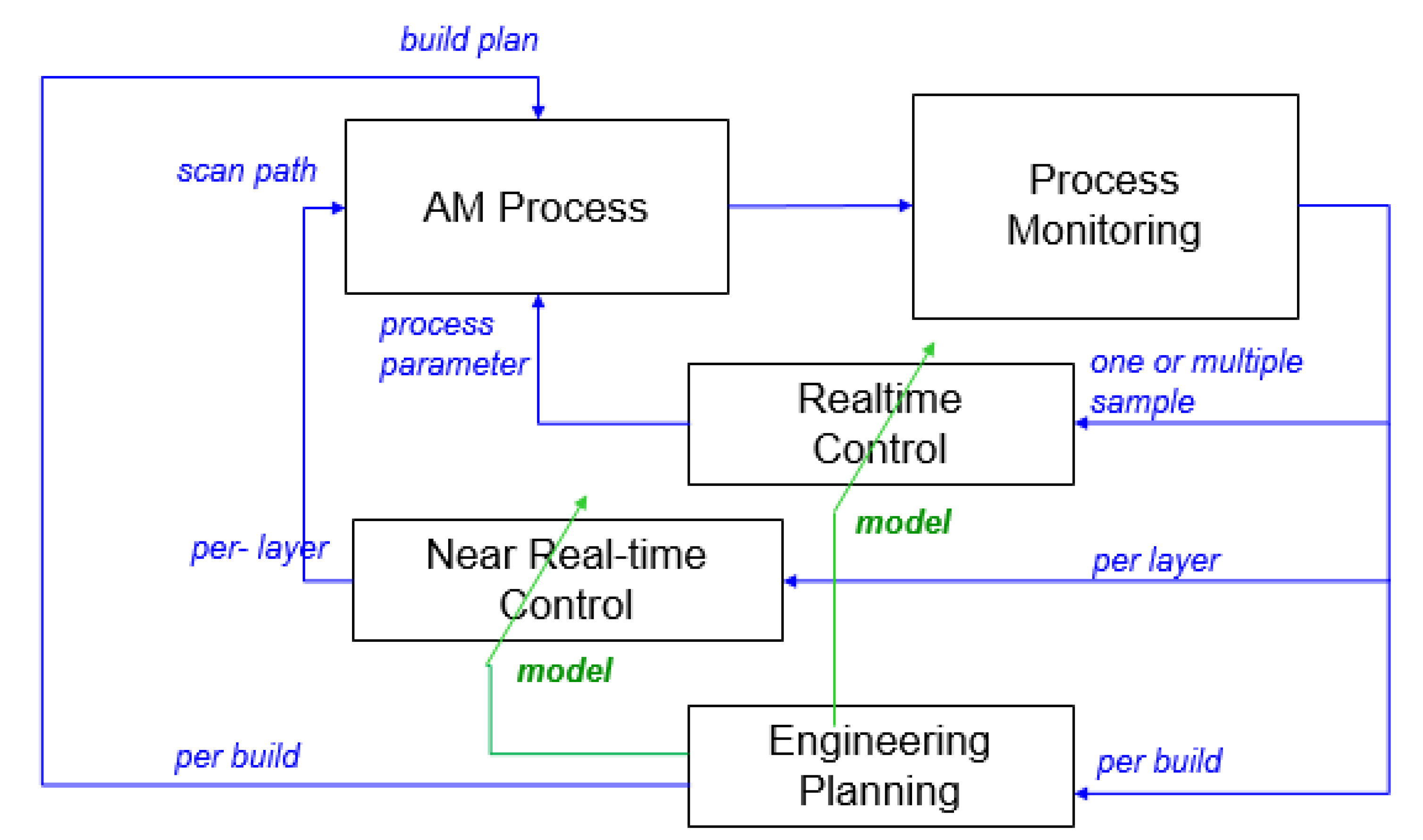
To utilize the capabilities of the monitoring systems in Appendix A, we propose a multi-loop, time-based approach to AM-process control. Our proposed control architecture is shown in Figure 1. It has two internal temporal loops: a real-time loop and a near-real-time loop. The major input to this multi-loop controller is a build plan, which involves process-specific and machine-specific tasks. Process-specific tasks include choosing the required support lattices and build orientation. Machine-specific tasks include converting the build plan into the formats required by (1) the controller of the AM machine that will build the product and (2) the monitoring systems that come with that machine. Today, that conversion is usually done by machine-specific, software tools.
The real-time loop uses individual samples of in situ, melt-pool data to monitor and control the process parameters. Changes in those parameters will be needed if the analysis of that sample data indicates an unstable process. The “sample-based” feedback data includes melt-pool temperatures and sizes, sampled at up to 20 kHz. The sample-based, process-control parameters include energy power and material-feed rates. As of today, only a few AM machines have the capabilities to execute this real-time, control loop. The near-real-time, layer-wise loop determines the scan path and process parameters for the next layer based on the entire collection of sample-based monitoring data.
Process monitoring includes functions to curate, fuse, and communicate in situ sensor/measurement data for both control loops. These functions are computationally rigorous outside the competence of the traditional, edge-computing nodes, such as PLCs or embedded controllers. Today, physics-based predictive models are rarely used in AM. Therefore, the predictive models used for both inner- and outer-loop control are previously trained, offline, data-driven AI/ML models. The major output of the loop-based monitoring functions, therefore, are the information models needed as inputs to those AI/ML models [12,13,14,15,16,17].
In the following sections, we provide more details about the functions inside each control loop and the some of the offline functions needed to provide the models used in those functions.
4. A Closer Look at the Time-Based Functions
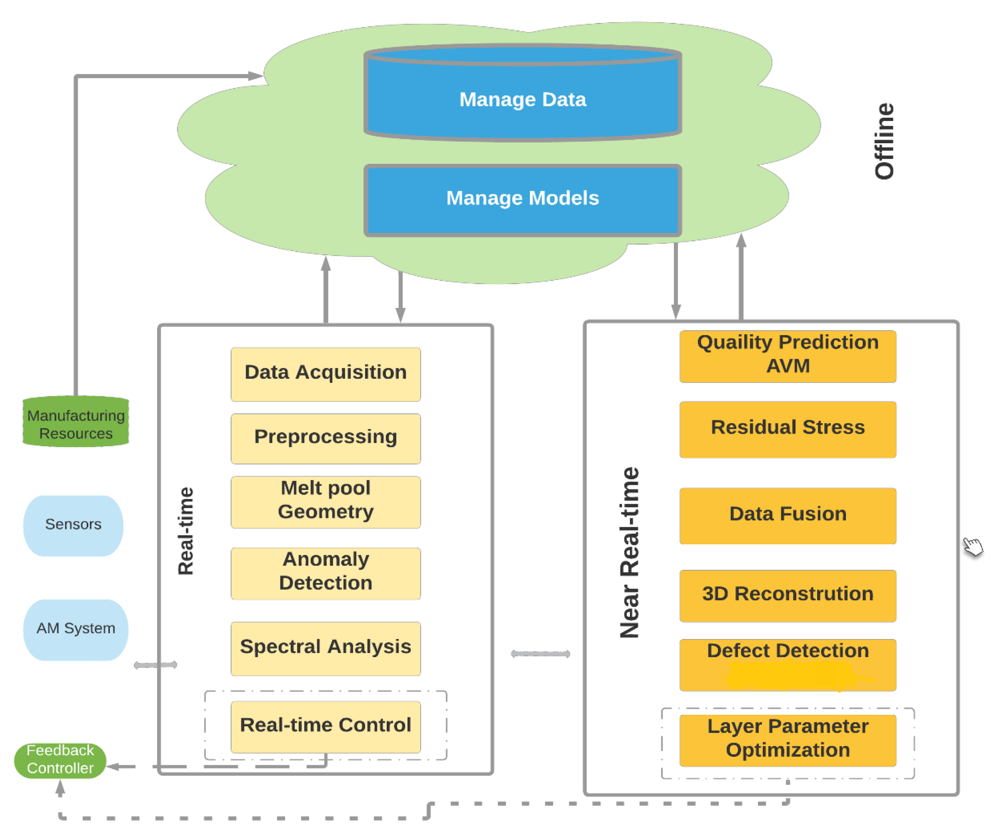
Figure 2 shows the internal, real-time, near-real-time, and offline control functions. Real-time, internal-loop, control functions include (1) acquiring sensor data from the various in situ monitoring sensors, (2) cleaning and tagging that data, (3) analyzing that data to estimate the current characterization of the melt-pool, and (4) deciding what to do with that analysis. Common, data-driven, control decisions include keeping the current settings or changing them. A less common but more drastic control decision would be to stop the build process entirely (see Section 4.1).
Near-real-time functions use layer-wise, monitoring data as input to data-analytics and AI tools to control both the process stability and the part quality. Before creating that input, all process-monitoring data from previous layers must be fused. Before using that fused data, it must be transformed into the syntax and semantics required by the chosen analysis tool. The two, near-real-time control decisions are the scan-path and energy-intensity settings. If the data analysis shows no problem, then the scan path remains the same. If a problem is detected and the decision is to continue the build, then a new scan strategy must be selected based on its predicted impact on the part quality. New process parameters might be needed as well. Section 4.2 provides more detail [18].
4.1. Real-Time Function Loop
The real-time functions include data acquisition, preprocessing, process-parameter selection, melt-pool feature extraction, and anomaly detection. Data includes melt-pool temperature measurements, melt-pool images, process settings, and actual laser-power measurements. The preprocessing function is necessary to remove noise from data samples, noise that will result in the uncertainty in the final measurements. Since process parameters play an important role in part quality, their selection is critical. Their selection is also not an easy task due to the dynamic and uncertain natures of both the AM materials and the AM process. Those natures mean that parameters controlling AM processes cannot be fixed during the process. If parameters such as laser power levels and scan speed are fixed, overheating and underheating occurs during fabrication, for example, for the nonconventional continuous scan strategy [19]. Therefore, most process parameters must be set initially and then adjusted based on those real-time measurements. Adjustments can be made manually or by using esoteric optimization techniques such genetic algorithms and self-organizing maps [20].
Melt-pool-geometry measurements are used to control the process and to predict the quality of the AM part. The following steps are taken to measure the geometry of melt-pool: (1) remove the noise from images using a either a 3 × 3 or 5 × 5 Gaussian filter, (2) find the edge of melt-pool using Canny [21] or any other method for edge detection, and finally (3) calculate the area of melt-pool by fitting ellipses or rectangles or otherwise measuring size of the pool. The melt-pool geometry can be used to predict when the process is outside its normal operating range. Based on a defined threshold, the geometry can also detect anomalies during the AM process. Some researchers use other methods, such as bag-of-words, k-means unsupervised clustering, and convolutional neural networks for anomaly detection and classification in LPBF processes [22,23].
The real-time control functions continuously reoptimize the process parameters based on the measurement-data analysis. For this type of optimization, different machine learning algorithms, such as genetic algorithms and artificial neural network (ANN), are commonly used [20].
4.2. Near-Real-Time Function Loop
Near-real-time functions include sensor-data fusion, residual-stress estimation, 3D Optical coherence tomography (OCT) model reconstruction, defect detection, process-parameter selection, and part-quality prediction. Today’s AM machines are instrumented with a myriad of sensors often from third party vendors. Those sensors collect and communicate a large variety of high-dimensional data over extremely short periods of time. Typically, tens of thousands of images are collected using high-speed cameras. Large, field-of-view, staring cameras produce several high-definition, global images of each layer. All this sensor data must be fused before the other functions can be executed. Sensor-data fusion is still a major area of research [24,25]. Fused images, machine-control commands and other sensor measurements are necessary for this control loop. Consequently, the computational requirements to perform near-real-time functions are very high.
One of those requirements includes making an accurate, residual stress estimation, which is used to obtain the maximum dimensional accuracy and to avoid early fatigue failure [26]. Many process parameters affect the residual stress in AM [27]. Estimation results are used as inputs to optimize the scan-path and process parameters for the next build layer.
Another requirement is defect detection, which is based on both 3D Optical coherence tomography (OCT) and dimension analysis at all layers of the part. Due to its high resolution and nondestructive nature, OCT is also useful for surface-void detection, loose-powder detection, and subsurface-feature detection. OCT is also used to find cracks and areas of un-melted powder [28,29].
Finding defects on layer-wise images is critical so that we can choose more appropriate process parameters for the next build layer. Many existing methods can be used to find defects such as ANN, Bayesian classifier, support vector machines (SVM), and Convolutional Neural Networks (CNN). CNNs got attention due to its accuracy and fast execution time as compared to other approaches. The execution speed of a CNN is improved by using high-performance computing resources such as an advanced GPU. The productivity of these techniques can be used for (layer-wise) process control, supplementary process decisions, or remedial actions [30,31,32]. Some investigators use an acoustic signal for in situ quality estimation in AM using deep learning [32,33].
4.3. Offline Modeling Functions
There are two offline functions: data management and model management. Much of the software needed to execute these functions are morphing to service in the cloud. Those services can perform big-data analysis, knowledge mining, decision support, regular maintenance, and long-term data storage. In addition to services, cloud computing provides some tremendous benefits such as virtualization, scalability, on-demand self-service resource pooling, and location freedom. Due to the massive amount of data generated in the AM process, latency and bandwidth considerations make it impossible to use the cloud for real-time system monitoring and control. In our purposed architecture, AM systems use the results of high-performance cloud computing for training purposes based on long-term, stored data [35].
4.3.1. Data Management
Data management focuses on an effective and efficient way to ensure that AM data are captured, stored, and used appropriately. The Senvol Database [36] provides researchers and manufacturers with open access to data related to industrial AM machines and materials. Granta, a material information management technology provider, offers the product GRANTA MI:Additive Manufacturing, specifically customized for AM data capturing and use [37].
At the same time, multiple database and data-management systems must be built to organize and manage the data generated from research and industry projects. The DMSAM (Data Management System for Additive Manufacturing) was developed by researchers at Penn State university to store and track all the data and information related to an AM part. NIST’s Additive Manufacturing Materials Database (AMMD) is a data management system built with NoSQL (Not Only Structured Query Language) database technology and provides a Representational State Transfer (REST) interface for application integration. The database captures rich, research datasets generated by the NIST AM program based on an open Extensible Markup Language (XML) schema [38].
In addition, as an open data management platform, the AMMD data management system is set to evolve through codevelopment of the AM schema and contributions of data from the AM community. To leverage the strength of all these database tools, a multi-tier AM collaborative data management system is needed with (1) distributed data storage facilitated by using common data terms and definitions, (2) collaborative linked data based on neutral data formats, (3) continuous knowledge management by extracting AM material process–structure–property relationships automatically from AM data, (4) lifecycle and value chain-based decision support, and (5) an adaptive data-generation system that helps the AM community to design experiments more efficiently. A collaborative, data management system is set to identify, generate, curate, and analyze AM data throughout the entire AM product lifecycle and can significantly reduce the cost and time associated with AM product deployment.
4.3.2. Model Management
Model management is essentially a model training process done in the cloud layer in the training and update function. Based on the recommendation from optimization and design functions, the training process for models can be done. All trained models are deployed to subsequent layers as per the control architecture. Based on both real- and near-real-time monitoring and analysis of sensor data, training functions can be used for training at an initial level to deploy the model in sublayers. If the predicted result does not match the current standards, the retraining function starts again to improve modeling accuracy.
Model management focuses on using data analytics to improve control decisions. In situ monitoring and control data from multiple builds as well as part development lifecycle data are aggregated for analysis. The data can be used for training to correlate process settings with process signatures, microstructure properties, and mechanical properties. The resulting models are used for build-plan generation. Machine learning can also be used to train models, which are used in real- or near-real-time process monitoring and control.
4.4. Interfaces
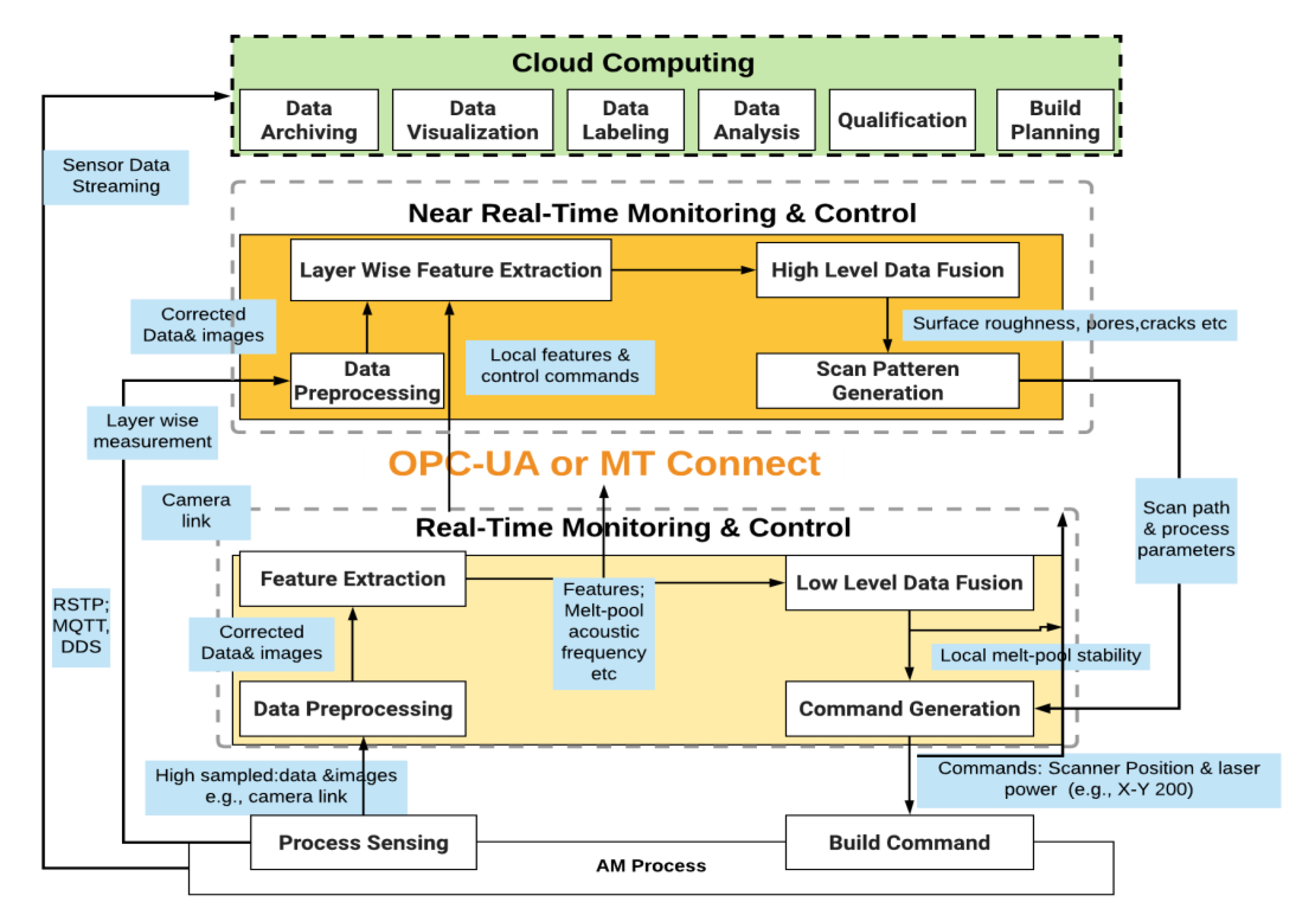
Figure 3 shows the data exchanged between function blocks and the applicable data-connection standards. For real-time control, sampled data or images are used to adjust the energy-input intensity which helps to control melt-pool formation and cooling. Real-time functions usually perform preprocessing, anomaly detection, and feature extraction on a per sample basis. Only extracted feature data is transferred to near-real-time functions. For the connections between control loops and IT systems, including the cloud, communication protocols are adopted by the AM machine vendors including OPC UA, MTConnect [39], and other Internet of Things standards.
OPC Unified Architecture (OPC UA) is a new generation standard from the OPC foundation with a wide, install base in traditional manufacturing plants. Some AM system vendors have already adopted OPC UA to monitor the operational status of their machines. MTConnect is a manufacturing technical standard for communicating process data from numerically controlled machine tools to shop-floor control systems. AM system vendors are investigating MTConnect for process monitoring; but currently, it is a read-only protocol control. Emerging internet of things (IoT) standards are playing an important role to communicate in situ monitoring data. Many standardized session layer protocols, like Message Queue Telemetry Transport (MQTT), Constrained Application Protocol (CoAP), and Data Distribution Service (DDS), can be applied in the AM domain to get measurements from monitoring devices. The Real Time Streaming Protocol (RTSP) is a network-layer protocol designed to control streaming media servers which are used to establish and control exposure surface or melt-pool image recording.
5. Case Study: In-Process Melt-Pool Monitoring
5.1. The AM System
The case study dataset was generated at the Additive Manufacturing Metrology Testbed (AMMT) at the National Institute of Standards and Technology (NIST) [4]. The AMMT is a fully custom-made metrology instrument that permits flexible control and measurement of the LPBF process. An internally developed AM software (SAM) program [40] was used to evaluate different scan strategies. In this study, an altered scan strategy was selected.
Wrought nickel alloy 625 powder and substrate, with a dimension of 4” × 4” × 0.5”, was used in this case study. Twelve rectangular parts (with chamfered corners) of dimensions 10 mm × 10 mm × 5 mm were laid on the substrate, with a minimum spacing of 10 mm between parts. In-process monitoring was based on two cameras: one high-resolution camera for layer-wise images and a high-speed camera to get the melt-pool images. The Galvo mirror system and the beam splitter permit the high-speed camera to focus on the current, laser-melting spot. Emitted light from the melt pool, through an 850-nm bandpass filter (40 nm bandwidth), was imaged on the camera sensor. The trigged time of the melt-pool camera was 500 μs.
5.2. Our Chosen Control Problem
In this study, we focus on near-real-time, sometimes called layer-wise, control of the melt-pool size (see Section 5.3). The time constraint for layer-wise control is defined in the equation below.
where
- : layer-wise melt-pool classification;
- : time to record the coaxial camera melt-pool video;
- : time to extract the features of melt-pool;
- : time to perform clustering on melt-pool area; and
- : recoating powder time for next layer.
For layer-wise monitoring of melt-pool size, the data must be collected and analyzed before the next layer of printing begins. Since the inter-layer, powder-recoating time takes approximately 10 s [41], both must be completed within the recoating time frame. In the melt-pool size analysis case study, collecting melt-pool data from one layer takes 1 s. It is likely to extract the features within 3 s by using a parallel-computing technique, and our clustering method takes round about 0.80 s. All of this is described in the following sections.
Therefore, the total time cost is less than 5 s, which is plenty of time for a decision to be made based on that analysis. It means that there is 5 s left to make control decisions based on that analysis. Those decisions include (1) doing nothing or (2) changing the laser power and/or the scan speed, which are known to impact melt-pool size estimated using the melt-pool area. If the area is too big or too small, it means that the AM process is not stable. This is turn indicates a part-quality problem.
5.3. Melt-Pool Size: A Near-Real-Time Control Problem
The current case study focuses on controlling the size of the melt pool, which as noted, is a part of real-time loop in our architecture. We collected data from two different layers during the build, called layer1 and layer2. The total number of real-time, melt-pool samples consists of 2269 and 2215, respectively. Control decisions are based the results of melt-pool size monitoring and defect detection. If the process is stable, we assume that the part quality, which is determined from the specifications provided by the user, is acceptable. In the remainder of this section, we discuss our proposed, automatic, two-staged detection method to estimate the melt-pool size using that data automatically.
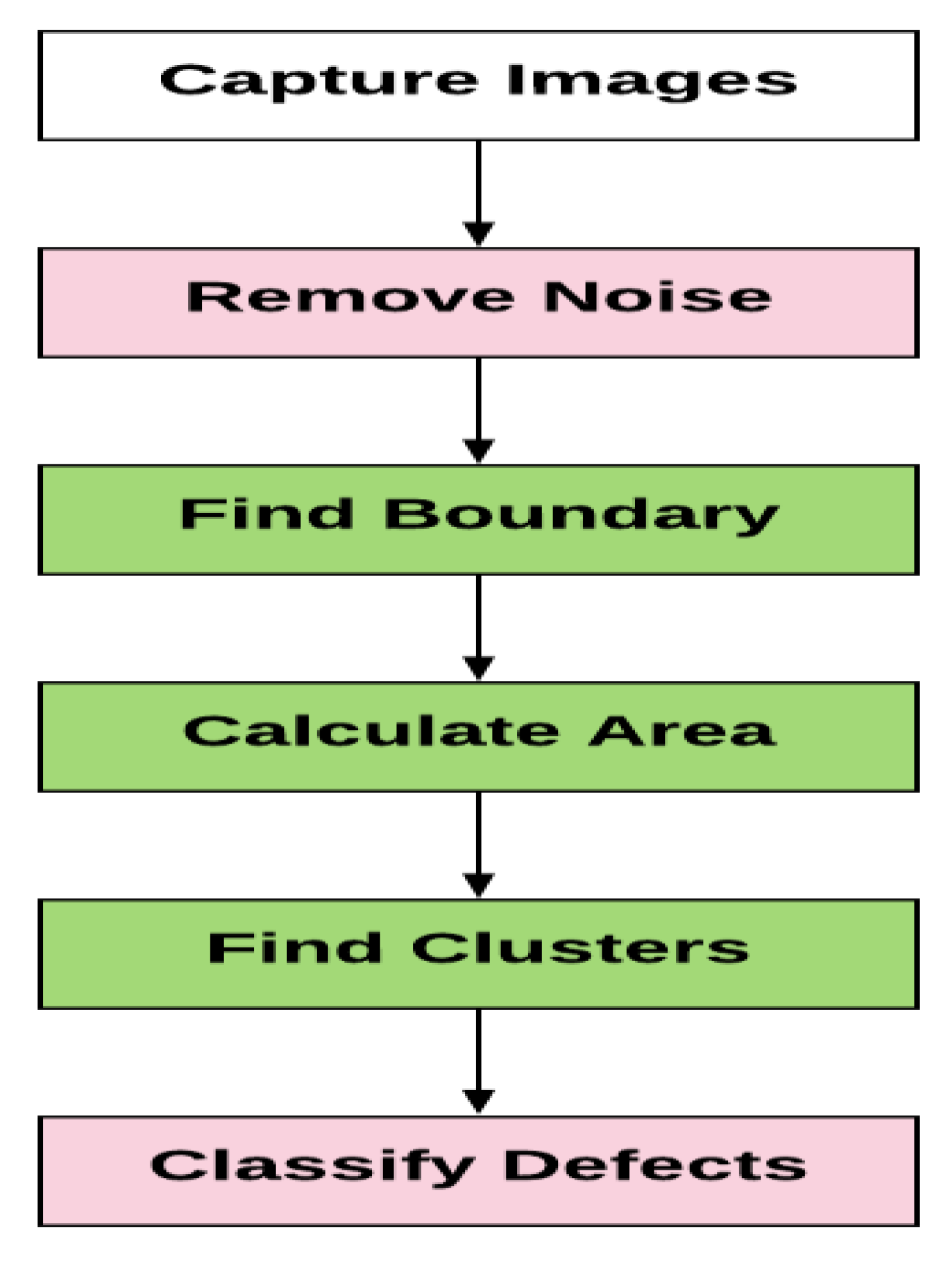
The defect detection process is shown in Figure 4. After capturing the melt-pool images, the first step is to remove any noise in the images. We chose the Gaussian filter, which is a well-known noise- removal process. The next step is to find the structural boundary of the melt pool, which we used the canny edge detection method [21]. After the boundary of the melt-pool is known, the width, length, and area of the melt-pool can be calculated.
Based on the area, we use a K-means clustering techniques to find any defects.
5.4. Analyzing Data
We used a K-means clustering algorithm to find the possible geometric-shape and defect patterns that can arise in the melt pools created during the build on which this study is based. K-means clustering is one of the famous algorithms for finding such patterns. K-means algorithm divides the dataset into predefined “clusters”, with the property that each data point belongs to one, and only one, cluster. The algorithm attempts to make each cluster have approximately the same number of data points [42]. It allocates the data points to a cluster by minimizing their Sum-of-Square distance (SSD). We chose to minimize SSD based on the idea that, the more similarity among the data points (the lower the SSD, the likelier it is that they belong in the same cluster.
These clusters become the basis for creating the two previously mentioned patterns: shape or defect. The next step is to identify which cluster belongs to which pattern, but first, we provide the algorithm.
5.4.1. K-Clustering Algorithm
The k-means algorithm works as follows Algorithm 1 [43].
| Algorithm 1 K-Means |
|
We calculate the centroids for the clusters by taking the average distance between all cluster data points. We used random initializations of the algorithm to minimize its effects by choosing the initialization that has the least SSD distance as the centroid. We chose K-means clustering because it is repetitive in nature and can handle random start initializations. There is one potential drawback. The specific, software implementations of that algorithm may get stuck in a local optimum and, therefore, will not converge to the global optimum [43].
The objective function is as follows:
where wik = 1 for data point xi if it belongs to cluster k; otherwise, wik = 0. Also, μk is the centroid of xi’s cluster.
5.4.2. Find the Number of Clusters Automatically in the Dataset
There are two well-known methods to find the appropriate number of clusters automatically: the elbow method and silhouette-analysis method [44]. In this study, we used the elbow method. The elbow method gives us a suitable (k) number of clusters based on the SSD between individual data points and the proposed centroid of the cluster. Algorithm (1) runs several times over the loop by increasing the number clusters and then (2) plots each proposed cluster’s score as a function of the number of clusters. Elbow method can be articulated by SSD in the equation below [44].
with k = many clusters formed, Ci = the ith cluster, and x = the data present in each cluster. The elbow method is used to find the value of (k) number of clusters in the given data set.
5.5. Applying Clustering to our Melt-Pool Monitoring Problem
There are still many challenges that exist for monitoring and controlling the AM process. Melt-pool-shape monitoring is one of the key features used for quality estimation in AM. In-situ-based, monitoring systems are reliable approaches used by different researchers for real-time melt-pool monitoring. A high-speed camera is used to monitor the melt-pool in real-time during the AM manufacturing process.
After capturing the melt-pool images during manufacturing, the next step is to remove the noise and to extract the key features from the melt-pool. Completing these two functions in a timely manner is another challenge for real-time feedback control. In our case, in the next step, we needed to find the boundary of the melt-pool to estimate its area. After estimating the area, we used the elbow method to find the number of and members of clusters automatically within that area. The k-means methods clusters nearby points to find defects in the melt-pool.
In addition to the part quality, the melt-pool provides important information about the stability of the AM process. Based on the melt-pool shape, we can predict whether the AM process is functioning normally. Two principal parameters that affect the shape of the melt-pool are laser power and scan speed. It is possible to readjust these parameters based on the melt-pool-shape analysis. It means that, by monitoring the melt-pool size and shape, we can make control decisions that will positively impact the quality of the fabricated AM part.
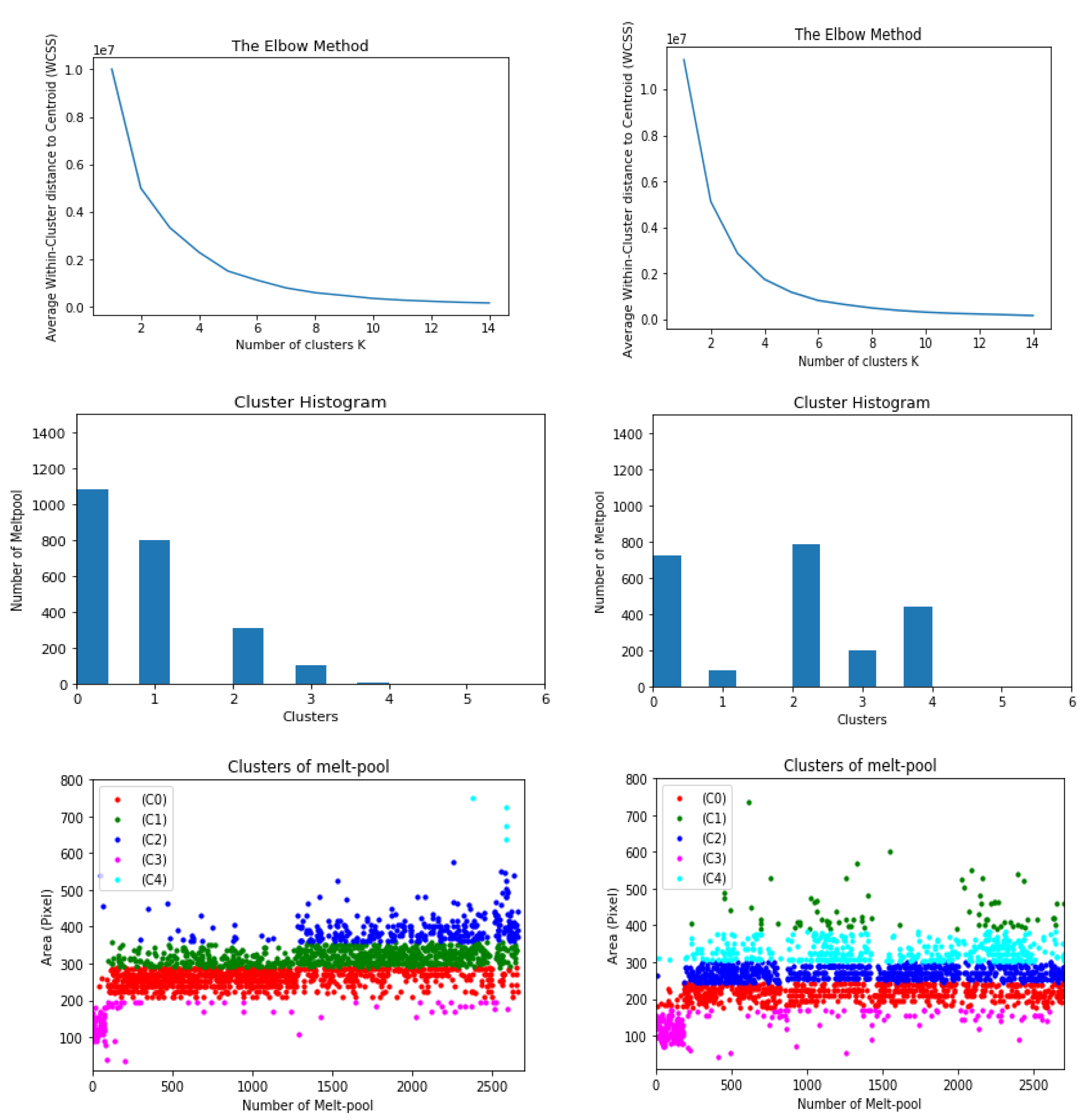
As noted above, since our focus in this study is near-real-time control, we use the K-means Cluster algorithm on two different build layers called layer1 and layer2, with 2269 and 2215 data points, respectively. We used each layer’s data points and their associated melt pool area as inputs to the elbow method. We used this method to find the appropriate number of clusters (see Figure 5). For layer1, the optimal number of clusters is shown in the left top Figure 5. By observing each cluster’s shown histogram, we find that, in clusters C2, C3, and C4, the shapes and sizes of the corresponding melt-pool shapes are very different from the other histograms.
Therefore, these clusters are considered abnormal and represent two patterns of defects. Based on the very high values of C2 and C4 (drawn in blue and cyan color in the left bottom figure), their likelihood of being real defects is quite high. Given the value for C3, its likelihood is much lower. From the perspective of near-real-time control, these patterns must be identified and their quality impact must be assessed before any decision can be made.
5.6. Example Results
The right side of Figure 5 shows the result on the layer 2 dataset of the melt pool. The number of MPs in clusters C1 and C3 is fairly less compared to other clusters. It can be understood that these melt-pools are very different in size and shape from other MPs. The area of these MP (C1 and C3) is either very high or low as compared to other MPs, as shown in the right bottom figure of the cluster of MPs. The guess estimation of this clustering-based, defect-detection method is that these melt-pools belong to be anomalies, splashes, etc.
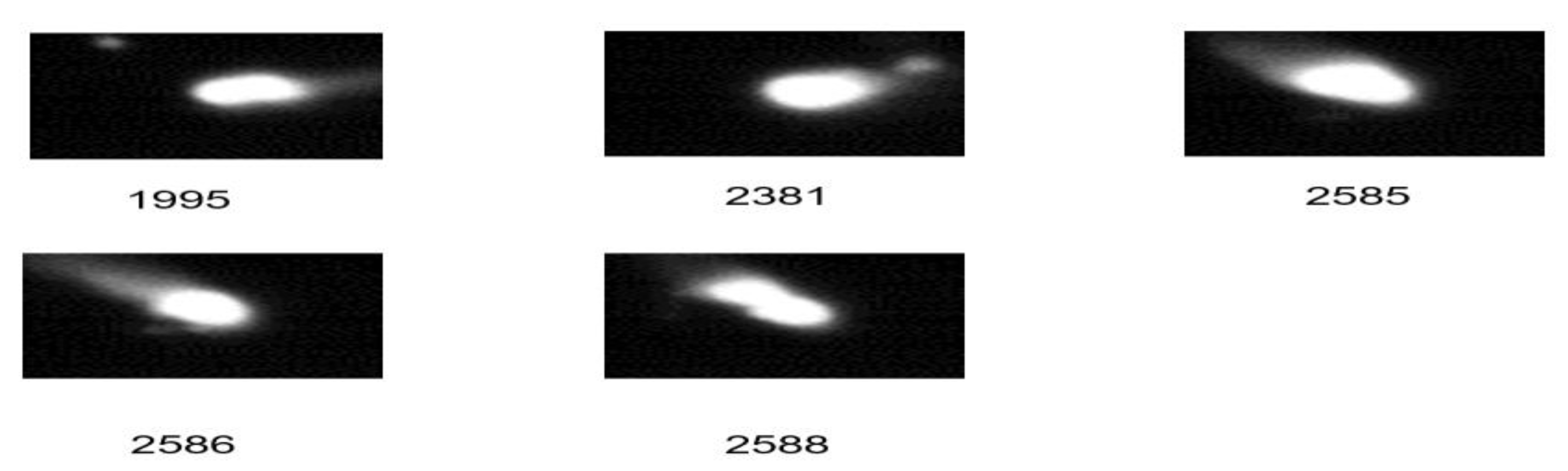
To check the accuracy of the proposed approach, we observe the bottom left of Figure 5 for clustering and we find that the (C4) cluster color cyan shows that this cluster has only a very few number of melt pools as compared to other melt pool. When we cross-check the C4 cluster in their original image dataset, we find that this melt pool is abnormal and its melt pool shape is a fairly big area as compared to other clusters, as shown in Figure 6. Similarly, the bottom right figure of the clustering shows that C1 and C3 has a few number of melt pools, which means that these melt pool also belongs to defects.
6. Summary
This paper proposes a functional architecture for controlling AM processes. That architecture has two internal control loops: real-time and near-real-time. Real-time functions include data acquisition, preprocessing, curating, and tagging from in situ sensors. Data analysis focuses on using individual samples to characterize the melt pool for small collections of that data. Near-real-time functions focus on individual layers. Those functions include data fusion, residual stress estimation, 3D opaque model reconstruction, defect detection, and part quality prediction. The outer-most, layer-wise loop is for near-real-time control. This loop makes adjustment of scan path and process parameters for the next layer based on the monitoring information from the previous layers.
In addition to these internal, control-loop functions, the paper discusses some of the offline functions associated with training and retraining the AI/ML models used by those analysis functions. The paper includes an example of a near-real-time, control function: melt-pool size. It describes both the collection method and the analysis methods. There are two methods: the K-means clustering method and the elbow method. The elbow method determines the optimal number of clusters, and the clustering method identifies which data points go in which cluster. The melt-pool area for each cluster is the control metric. The area of each cluster is calculated; based on the area (too big or too small), defects are determined. Control decisions, such as changing the laser power and scan speed, can be made based of the area.
7. Disclaimer
Certain commercial systems are identified in this paper to facilitate better understanding. Such identification neither implies recommendation or endorsement by NIST nor implies that the products identified are necessarily the best available for each purpose. Further, any opinions, findings, conclusions, or recommendations expressed in this material are those of the authors and do not necessarily reflect the views of NIST or any other supporting U.S. government or corporate organizations.
Author Contributions
Conceptualization, M.A., Y.L., A.J., H.Y., and F.-T.C.; methodology, M.A., A.J., and H.Y.; investigation, M.A. and Y.L.; resources, Y.L.; writing—original draft preparation, M.A.; writing—review and editing, Y.L., A.J., and H.Y.; supervision, A.J., Y.L., and F.-T.C.; project administration, Y.L. All authors have read and agreed to the published version of the manuscript.
Funding
This research was funded by the “Intelligent Manufacturing Research Center” (iMRC) from The Featured Areas Research Center Program within the framework of the Higher Education Sprout Project by the Ministry of Education (MOE) in Taiwan.
Acknowledgments
This work was partially supported by the “Intelligent Manufacturing Research Center” (iMRC) from The Featured Areas Research Center Program within the framework of the Higher Education Sprout Project by the Ministry of Education (MOE) in Taiwan.
Conflicts of Interest
The authors declare no conflict of interest.
Appendix A
In Appendix A, Table A1 shows some commercially available monitoring systems. SLM solutions provide an on-axis monitoring system by using two diodes, but the Concept Laser systems use one diode and one camera integrated using the on-axis technique. Sigma Labs developed the system based on on-axis and off-axis photodiode joints with an off-axis pyrometer incorporated straight into the building chamber. Stratonics Inc. uses a CMOS-based 2-gamma-pyrometer camera that covers only the building platform and can incorporate either on-axis or off-axis. Renishaw developed the InfiniAM Spectral system, which is an on-axis system of an “Infrared thermal sensor (1090 nm to 1700 nm)” and a “near infrared plasma sensor (700 nm to 1049 nm)”. The Renishaw camera, which covers only the building platform, can be used either on-axis or off-axis. EOS developed the EOSTATE monitoring system which is a combination of EOSTATE MeltPool as on-axis and photodiode-based system that is an off-axis camera-based system [45].

Table A1.
Commercial monitoring systems.
| Vendor | Product | Features | Sensors | FPS | Pixel Size | Filter | Real-Time |
|---|---|---|---|---|---|---|---|
| Concept Laser | QM meltpool 3D | melt pool (area and intensity) | Co-axial camera and photodiode | Camera 10 kHz & photodiode-50 kHz | 35 µm | 1070 nm | Data available after the build process (offline) (No Feedback) |
| Concept Laser | QM coating | powder bed surface | Off-axis camera | ||||
| EOS | EOSTATE meltpool | melt pool | Co-axial and off-axial photodiode | Sampling 60 kHz | 50 µm/pixel | 1064 nm | Real-time only melt-pool analysis (No Feedback) |
| EOS | EOSTATE powder bed | powder bed | Off-axial camera | ||||
| EOS | EOSTATE OT | Quality issues | Off-axial camera | 10 fps | 125 µm/pixel | Real-time (layer by layer) (No Feedback) | |
| Renishaw | InfiniAM | Energy input & melt-pool emissions monitoring | Infrared thermal sensor & near infrared plasma sensor on-axis | 100 kHz | 300–700 nm & 700–1700 | Real-time analysis (layer-by-layer) (no feedback) | |
| Stratonics Inc | ThermaViz | Meltpool sensor | CMOS base 2-gamma-pyrometer-camera | 25 fps | 10 µm/pixel | near real-time analysis | |
| Sigma Lab | PrintRite3D | Melt pool area Thermal intensity | Pyrometer | 200 kHz | 100 µm/pixel | layer wise monitoring |
References
- Vandone, A.; Baraldo, S.; Valente, A. Multisensor data fusion for additive manufacturing process control. IEEE Robot. Autom. Lett. 2018, 3, 3279–3284. [Google Scholar] [CrossRef]
- Frazier, W.E. Metal additive manufacturing: A review. J. Mater. Eng. Perform. 2014, 23, 1917–1928. [Google Scholar] [CrossRef]
- 3Dnatived. Available online: https://www.3dnatives.com/en/metal-3d-printer-manufacturers/ (accessed on 31 July 2019).
- Lane, B.; Mekhontsev, S.; Grantham, S.; Vlasea, M.; Whiting, J.; Yeung, H.; Fox, J.; Zarobila, C.; Neira, J.; McGlauflin, M.; et al. Design, developments, and results from the nist additive manufacturing metrology testbed (ammt). In Proceedings of the Solid Freeform Fabrication 2016—27th Annual International Solid Freeform Fabrication Symposium—An Additive Manufacturing Conference Solid Freeform Fabrication Symposium, Austin, TX, USA, 8–10 August 2016. [Google Scholar]
- OPC-UA. Available online: https://opcfoundation.org/about/opc-technologies/opc-ua/ (accessed on 18 September 2020).
- Yang, H.-C.; Adnan, M.; Huang, C.-H.; Cheng, F.-T.; Lo, Y.-L.; Hsu, C.-H. An Intelligent Metrology Architecture with AVM for Metal Additive Manufacturing. IEEE Robot. Autom. Lett. 2019, 4, 2886–2893. [Google Scholar] [CrossRef]
- Grasso, M.; Colosimo, B.M. Process defects and in situ monitoring methods in metal powder bed fusion: A review. Meas. Sci. Technol. 2017, 28, 044005. [Google Scholar] [CrossRef] [Green Version]
- Toeppel, T.; Schumann, P.; Ebert, M.C.; Bokkes, T.; Funke, K.; Werner, M.; Zeulner, F.; Bechmann, F.; Herzog, F. 3D analysis in laser beam melting based on real-time process monitoring. In Proceedings of the Materials Science and Technology Conference, Salt Lake City, UT, USA, 23–27 October 2016. [Google Scholar]
- Stratonics. Available online: http://stratonics.com/wp-content/uploads/2016/03/ThermaViz-Operating-Manual-2015.04.03.pdf (accessed on 31 July 2019).
- Stratonics. Available online: http://stratonics.com/systems/software/ (accessed on 31 July 2019).
- Renishaw. Available online: https://www.renishaw.com/en/infiniam-spectral--42310 (accessed on 31 July 2019).
- Asiltürk, I.; Çunkaş, M. Modeling and prediction of surface roughness in turning operations using artificial neural network and multiple regression method. Expert Syst. Appl. 2011, 38, 5826–5832. [Google Scholar] [CrossRef]
- Vahabli, E.; Rahmati, S. Application of an RBF neural network for FDM parts’ surface roughness prediction for enhancing surface quality. Int. J. Precis. Eng. Manuf. 2016, 17, 1589–1603. [Google Scholar] [CrossRef]
- Zhang, J.; Wang, P.; Gao, X.R. Modeling of Layer-wise Additive Manufacturing for Part Quality Prediction. Proc. Manuf. 2018, 16, 155–162. [Google Scholar] [CrossRef]
- Markl, M.; Körner, C. Multiscale modeling of powder bed–based additive manufacturing. Ann. Rev. Mater. Res. 2016, 46, 93–123. [Google Scholar] [CrossRef]
- Li, Z.; Zhang, Z.; Shi, J.; Wu, D. Prediction of surface roughness in extrusion-based additive manufacturing with machine learning. Robot. Comput.-Integr. Manuf. 2019, 57, 488–495. [Google Scholar] [CrossRef]
- Francis, J.; Bian, L. Deep Learning for Distortion Prediction in Laser-Based Additive Manufacturing using Big Data. Manuf. Lett. 2019, 20, 10–14. [Google Scholar] [CrossRef]
- Adnan, M.; Lu, Y.; Jones, A.; Cheng, F.T. Application of the Fog Computing Paradigm to Additive Manufacturing Process Monitoring and Control. In Proceedings of the Solid Freeform Fabrication Symposium an Additive Manufacturing Conference, Austin, TX, USA, 12–14 August 2019. [Google Scholar]
- Yeung, H.; Yang, Z.; Yan, L. A Meltpool Prediction Based Scan Strategy for Powder Bed Fusion Additive Manufacturing. Addit. Manuf. 2020, 35, 101383. [Google Scholar]
- Fathi, A.; Mozaffari, A. Vector optimization of laser solid freeform fabrication system using a hierarchical mutable smart bee-fuzzy inference system and hybrid NSGA-II/self-organizing map. J. Intell. Manuf. 2014, 4, 775–795. [Google Scholar] [CrossRef]
- Canny, J. A Computational Approach to Edge Detection. Readings in Computer Vision; Morgan Kaufmann: Burlington, MA, USA, 1987; pp. 184–203. [Google Scholar]
- Scime, L.; Beuth, J. Anomaly detection and classification in a laser powder bed additive manufacturing process using a trained computer vision algorithm. Addit. Manuf. 2018, 19, 114–126. [Google Scholar] [CrossRef]
- Scime, L.; Beuth, J. A multi-scale convolutional neural network for autonomous anomaly detection and classification in a laser powder bed fusion additive manufacturing process. Addit. Manuf. 2018, 24, 273–286. [Google Scholar] [CrossRef]
- Powder Bed Fusion Additive Manufacturing. In Proceedings of the Dimensional Optical Metrology and Inspection for Practical Applications IV, Baltimore, MD, USA, 20–21 April 2015; International Society for Optics and Photonics: Bellingham, WA, USA, 2015; 9489.
- Reutzel, E.; Abdalla, W.; Nassar, R. A survey of sensing and control systems for machine and process monitoring of directed-energy, metal-based additive manufacturing. Rapid Prototyp. J. 2015, 21, 159–167. [Google Scholar] [CrossRef] [Green Version]
- Mukherjee, T.; Zhang, W.; DebRoy, T. An improved prediction of residual stresses and distortion in additive manufacturing. Comput. Mater. Sci. 2017, 126, 360–372. [Google Scholar] [CrossRef] [Green Version]
- Fergani, O.; Berto, F.; Welo, T.; Liang, S.Y. Analytical modelling of residual stress in additive manufacturing. Fatigue Fract. Eng. Mater. Struct. 2017, 40, 971–978. [Google Scholar] [CrossRef]
- Guan, G.; Hirsch, M.; Lu, Z.H.; Childs, D.T.; Matcher, S.J.; Goodridge, R.; Groom, K.M.; Clare, A. Evaluation of selective laser sintering processes by optical coherence tomography. Mater. Des. 2015, 88, 837–846. [Google Scholar] [CrossRef]
- Guan, G.; Hirsch, M.; Syam, W.P.; Leach, R.K.; Huang, Z.; Clare, A. Loose powder detection and surface characterization in selective laser sintering via optical coherence tomography. Proc. R. Soc. A Math. Phys. Eng. Sci. 2016, 472, 20160201. [Google Scholar] [CrossRef]
- Aminzadeh, M.; Kurfess, R.T. Online quality inspection using Bayesian classification in powder-bed additive manufacturing from high-resolution visual camera images. J. Intell. Manuf. 2019, 30, 2505–2523. [Google Scholar] [CrossRef]
- Gobert, C.; Reutzel, E.W.; Petrich, J.; Nassar, A.R.; Phoha, S.; Christian, G.; Edward, W.R.; Jan, P.; Abdalla, R.N.; Shashi, P. Application of supervised machine learning for defect detection during metallic powder bed fusion additive manufacturing using high-resolution imaging. Addit. Manuf. 2018, 21, 517–528. [Google Scholar] [CrossRef]
- Ye, D.; Hong, G.S.; Zhang, Y.; Zhu, K.; Fuh, J.Y.H. Defect detection in selective laser melting technology by acoustic signals with deep belief networks. Int. J. Adv. Manuf. Technol. 2018, 96, 2791–2801. [Google Scholar] [CrossRef]
- Shevchik, S.; Kenel, C.; Leinenbach, C.; Wasmer, K. Acoustic emission for in situ quality monitoring in additive manufacturing using spectral convolutional neural networks. Addit. Manuf. 2018, 21, 598–604. [Google Scholar] [CrossRef]
- Cheng, F.-T.; Huang, H.-C.; Kao, C.-A. Developing an Automatic Virtual Metrology System. IEEE Trans. Autom. Sci. Eng. 2012, 9, 181–188. [Google Scholar] [CrossRef]
- Wu, D.; Terpenny, J.; Zhang, L.; Gao, R.; Kurfess, T. Fog-enabled architecture for data-driven cyber-manufacturing systems. In Proceedings of the ASME 2016 11th International Manufacturing Science and Engineering Conference, American Society of Mechanical Engineers, Blacksburg, VI, USA, 27 June–1 July 2016. [Google Scholar]
- Senvol Database. Available online: http://senvol.com/database// (accessed on 18 September 2020).
- GRANTA MI AM. Available online: https://www.grantadesign.com/industry/products/granta-mi/product-engineering/granta-miadditive-manufacturing/ (accessed on 18 September 2020).
- NIST AMMD. Available online: https://ammd.nist.gov/ (accessed on 18 December 2019).
- MTConnect. Available online: https://www.mtconnect.org/ (accessed on 18 September 2020).
- Yeung, H.; Lane, B.; Donmez, M. Implementation of Advanced Laser Control Strategies for Powder Bed Fusion Systems. Proc. Manuf. 2018, 26, 871–879. [Google Scholar] [CrossRef]
- Yang, H.-C.; Huang, C.-H.; Adnan, M.; Hsu, C.-H.; Lin, C.-H.; Cheng, F.-T. An Online AM Quality Estimation Architecture from Pool to Layer. IEEE Trans. Autom. Sci. Eng. 2020. [Google Scholar] [CrossRef]
- Kanungo, T.; Mount, D.; Netanyahu, N.; Piatko, C.; Silverman, R.; Wu, A. An efficient k-means clustering algorithm: Analysis and implementation. IEEE Trans. Pattern Anal. Mach. Intell. 2002, 7, 881–892. [Google Scholar] [CrossRef]
- K-Means Clustering: Algorithm, Applications, Evaluation Methods, and Drawbacks. Available online: https://towardsdatascience.com/20-practical-ways-to-implement-data-science-in-marketing-e10da4a6d0b2 (accessed on 3 February 2020).
- Syakur, M.A.; Khotimah, B.K.; Rochman, E.M.S.; Satoto, B.D. Integration k-means clustering method and elbow method for identification of the best customer profile cluster. IOP Conf. Ser. Mater. Sci. Eng. 2018, 336. [Google Scholar] [CrossRef] [Green Version]
- Fuchs, L.; Eischer, C. In-Process Monitoring Systems for Metal Additive Manufacturing; EOS Electro Optical Systems: Krailling, Germany, 2018. [Google Scholar]
Figure 1.
Multi-loop control architecture.

Figure 2.
Integrated functional models.

Figure 3.
Interfaces linking function blocks.

Figure 4.
Defect detection schema.

Figure 5.
Clustering result.

Figure 6.
Defected melt-pool images.

© 2020 by the authors. Licensee MDPI, Basel, Switzerland. This article is an open access article distributed under the terms and conditions of the Creative Commons Attribution (CC BY) license (http://creativecommons.org/licenses/by/4.0/).
Share and Cite
MDPI and ACS Style
Adnan, M.; Lu, Y.; Jones, A.; Cheng, F.-T.; Yeung, H. A New Architectural Approach to Monitoring and Controlling AM Processes. Appl. Sci. 2020, 10, 6616. https://0-doi-org.brum.beds.ac.uk/10.3390/app10186616
AMA Style
Adnan M, Lu Y, Jones A, Cheng F-T, Yeung H. A New Architectural Approach to Monitoring and Controlling AM Processes. Applied Sciences. 2020; 10(18):6616. https://0-doi-org.brum.beds.ac.uk/10.3390/app10186616
Chicago/Turabian StyleAdnan, Muhammad, Yan Lu, Albert Jones, Fan-Tien Cheng, and Ho Yeung. 2020. "A New Architectural Approach to Monitoring and Controlling AM Processes" Applied Sciences 10, no. 18: 6616. https://0-doi-org.brum.beds.ac.uk/10.3390/app10186616
Note that from the first issue of 2016, this journal uses article numbers instead of page numbers. See further details here.