Microseismic Signal Denoising and Separation Based on Fully Convolutional Encoder–Decoder Network


1
State Key Laboratory of Geohazard Prevention and Geoenvironment Protection, Chengdu University of Technology, Chengdu 610059, China
2
College of Environment and Civil Engineering, Chengdu University of Technology, Chengdu 610059, China
3
Department of Earth Sciences, University of Florence, 50125 Florence, Italy
4
Sichuan Yanjiang Panzhihua-Ningnan Highway Co., LDT, Xichang 615000, China
*
Author to whom correspondence should be addressed.
Appl. Sci. 2020, 10(18), 6621; https://0-doi-org.brum.beds.ac.uk/10.3390/app10186621
Submission received: 21 July 2020
/
Revised: 20 August 2020
/
Accepted: 21 September 2020
/
Published: 22 September 2020
(This article belongs to the Special Issue New Advance of Acoustic Emission and Microseismic Monitoring Technologies in Civil Engineering)
Abstract
:Denoising methods are a highly desired component of signal processing, and they can separate the signal of interest from noise to improve the subsequent signal analyses. In this paper, an advanced denoising method based on a fully convolutional encoder–decoder neural network is proposed. The method simultaneously learns the sparse features in the time–frequency domain, and the mask-related mapping function for signal separation. The results show that the proposed method has an impressive performance on denoising microseismic signals containing various types and intensities of noise. Furthermore, the method works well even when a similar frequency band is shared between the microseismic signals and the noises. The proposed method, compared to the existing methods, significantly improves the signal–noise ratio thanks to minor changes of the microseismic signal (less distortion in the waveform). Additionally, the proposed methods preserve the shape and amplitude characteristics so that it allows better recovery of the real waveform. This method is exceedingly useful for the automatic processing of the microseismic signal. Further, it has excellent potential to be extended to the study of exploration seismology and earthquakes.
1. Introduction
During monitoring and data acquisition processes, microseismic signals are often corrupted by various types of noise due to the uncontrollable sources, conditions, and complicated environmental situations. Possible noise could be electrical, construction, mechanical, or traffic noises. Spectral filtering is commonly used for improving the signal-to-noise ratio (SNR) of the microseismic signal. However, it is ineffective to suppress the noise that has a similar frequency band with a microseismic signal. Moreover, it can distort the signal [1] and/or generate artifacts before impulsive arrivals [2].
In order to alleviate this limitation, many methods have been proposed to suppress the noise in seismic/microseismic data, including Short Time Fourier Transform (STFT) [3], the Continuous Wavelet Transform (CWT) [4,5], S-transform [6], the Radon Transform [7,8,9], the Wave-Packet Transform (WPT) [10,11], Empirical Mode Decomposition (EMD) [12,13,14], Fuzzy methods [15], singular spectrum analysis [16], sparse transform-based denoising [17], mathematical morphology-based denoising approach [18], and the non-local means (NLM) algorithm [19]. Further, some hybrid methods were proposed, which combine the advantages of two or more denoising methods [20]. Signal denoising performance can be improved through two ways: a more effective sparse representation of the data and a more flexible and powerful mapping function. Although these methods mentioned above can properly suppress noise components in the data, it is still tricky to choose the optimal mapping function between the noisy signal and the estimated signal.
Recently, deep learning methods have been rapidly developed to overcome the drawbacks of the existing signal denoising methods. The deep neural network can learn extremely complicated mapping functions through the training, which has been proved to be a powerful tool for signal processing [21,22,23,24,25]. Inspired by the success of the encoder–decoder network for image/signal processing, a deep fully-convolutional encoder–decoder network is adopted (CNN-denoiser) for microseismic signals denoising. Given a noisy input signal, the CNN-denoiser can produce two masks (sparse representations): one for estimating signal and the other for estimating noise. Microseismic data recorded in the Micang Mountain tunnel in China are used for network training, validation, and testing. The method has also been tested with other noisy signals recorded in different actual projects, and semisynthetic signals (i.e., generated by superimposing microseismic signals and real noise) are also used to evaluate the proposed method in comparison to existing methods.
2. Methods and Network Training
2.1. Methods
The noisy signal, defined as , represents the superposition of real microseismic signals and noise that includes some instrumental noise or unknown noise in the time–frequency domain as follows:
where t and f represents the sampling point and frequency bins, respectively. The purpose of denoising is to minimize the expected error between the actual microseismic signal and the estimated microseismic signal :
where , is a function that maps to the , and n is the number of samples. In this paper, the error minimization problem is solved in a supervised learning manner in which a deep neural network learns to extract a sparse representation of noisy input waveform and to map it to a clean microseismic signal. The above theory is also used for estimation of noise, i.e.,. Then, the mapping functions are defined by two individual masks, modified from Zhu et al. [25], and for estimating microseismic signal and noise, respectively.
Both the two individual masks have the same sizes as the noisy signal , and they are merged as the targets for optimizing the performance of the neural network during training. Two masks contain a series of values between 0 and 1 to attenuate the noisy signal.
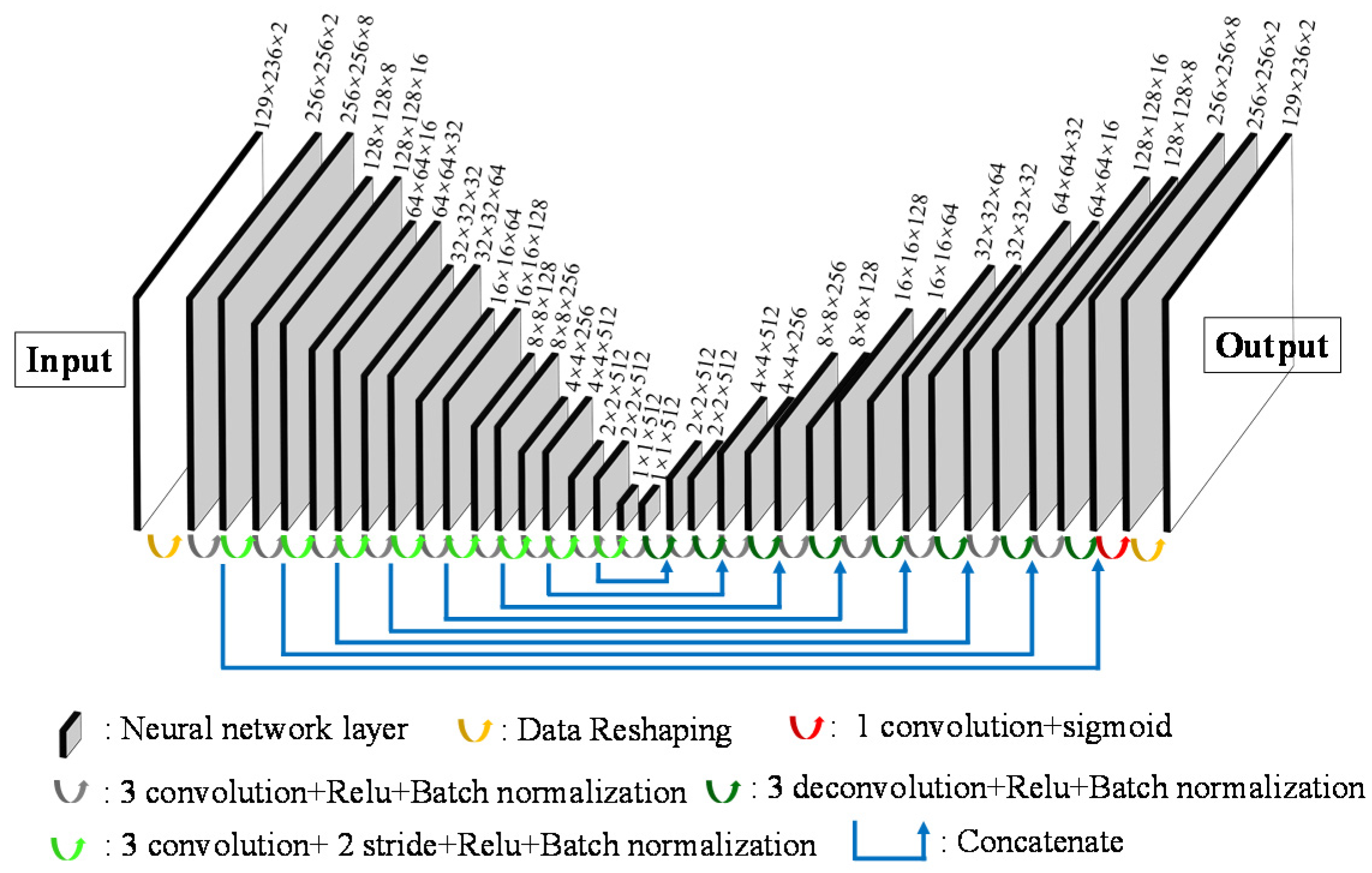
The real and imaginary parts of time–frequency coefficients of noisy signals (see Figure 1), as input vector, are firstly reshaped (from 129, 236, 2 into 256, 256, 2) by a zero-padding for the further encoding process. This is adapted from the existing method [25] to avoid a lack of noisy signal information in the encoding and decoding process. Otherwise, the feature space without reshaping will be shrunk by multiple downsampling operations (e.g., the shrinking process of the feature space as follows: 129, 236 firstly to 64, 118, then gradually to 32 and 59, 16 and 29, 8 and 14, 4 and 7, 2 and 3, and finally to 1, 1, which causes the loss of signal information, and the feature cannot be reconstructed entirely in the decoding process. The reshaped vector has then been transformed into new layers through a series of encoding operators that consist of a convolution, a ReLU (rectified linear unit) activation, and a batch normalization layer [26]. A stride of 2 is applied after every two successive layers to shrink the feature space gradually and improve the computational efficiency during the encoding process. For the convolution calculation, a larger kernel has a wider receptive field, which obtains more features of neighboring signals. However, the large convolution kernel leads to a dramatic increase in computational time limiting the depth of the neural network. Therefore, the kernel size of convolution/deconvolution layers is set to be 3 through the entire work. The decoding operators generate the masks and in the decoding process. The corresponding feature maps in the encoding and decoding process are concatenated with skip connections, which improve the convergence of training and the reconstruction information of signal [27]. In the penultimate layer of the denoising network, a softmax activation function is used to produce masks. In the last layer, the masks are reshaped into 129, 236, 2, where each channel represents the time–frequency coefficients of microseismic signal and noise, respectively.
Figure 2 shows the flow diagram of the proposed method. Firstly, the noisy signal is transformed into time–frequency domain using STFT. The real and imaginary parts of time–frequency coefficients of the noisy signal are input into the well-trained network. The network produces two masks for estimating both the time–frequency coefficients of microseismic signal and noise as outputs. The output masks are applied to the real and imaginary parts of time–frequency coefficients of noisy signal for producing the estimated time–frequency coefficients of the microseismic signal , and noise , respectively. Finally, the estimated microseismic signal and noise are obtained through inverse transforming and noise back into the time domain.
One of the advantages of the presented method is that instead of manually defining different features and thresholds to improve the SNR, it can automatically learn the richer features from the semi-synthetic noisy signals to obtain the estimated signals and noise in the time–frequency domain. Thus, deep learning has great potential to provide more efficient and accurate performance on signal denoising, which makes it possible to apply in other challenging tasks such as signal detection and onset time picking.
2.2. Data Preparation and Network Training
In this paper, 7500 microseismic signals with high SNRs and 15,000 noise samples were selected to form the dataset, which was randomly split into training (80%), validation (10%), and test (10%) datasets. The validation set is used to determine the hyperparameters and prevent over-fitting of the network from achieving the best results, and the test set is primarily used to evaluate network performance. The amplitude of the recorded signals is in voltage value, and the response frequency ranges from 50 to 5 kHz. The data acquisition station, located in the Micang Mountain tunnel in China, worked at the sampling frequency of 20 kHz and a sampling window of 1.5 s, which results in all signals having the size of 30,000 sampling points. The noisy input signal for training were generated through the training dataset and from the noisy signal with different SNRs by superimposing the selected microseismic signals with randomly selected noise samples on each iteration. The network was trained on NVIDIA GTX 1060 GPU with Adam optimizer and the learning rate of 0.001. Moreover, the noisy signals, recorded in the Zijing tunnel (China) by the microseismic monitoring system with the same parameters as Micang Mountain tunnel, were applied to the well-trained model for validating its versatility.
3. Results
3.1. Test Results
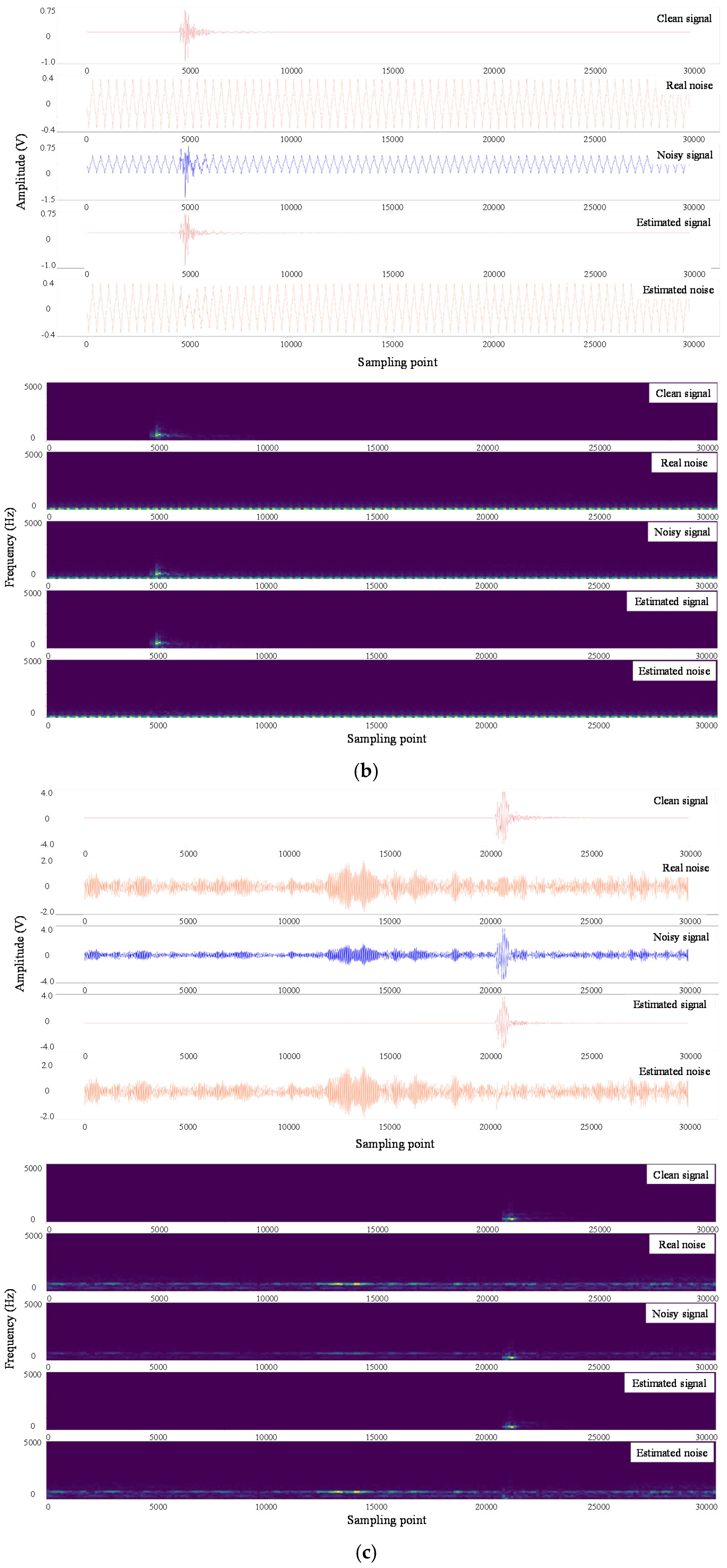
Figure 3 shows the denoised results of some noisy signals selected from the test dataset, which are obtained by applying the two output masks to these noisy signals. It is possible to observe that the method can successfully separate the noisy signal with different characteristics into an estimated signal and estimated noise. The CNN-denoiser has an excellent denoising performance for microseismic signals with various types and intensities of noise. Noisy signals in Figure 3a,b indicate microseismic signals with cyclic noise at different frequencies, and Figure 3c indicates microseismic signals with a mixture of cyclic and other noise. For the most part, the cyclic noise changes over time, and its frequency band overlaps with that of the microseismic signals, which is a challenging issue for existing denoising methods. These above types of noisy signals cover all the noisy signal samples in the field. It can be found that CNN-denoiser can effectively suppress the microseismic signals with non-Gaussian noise (including cyclic noise, unknown noise, and their mixture). To further demonstrate the applicability of the proposed method to other noise (like Gaussian noise), CNN-denoiser was tested in noisy signals formed with clean microseismic signal and Gaussian noise (Figure 3d). The results show that the noises are significantly reduced regardless of types of noise. Further, the estimated signal leakage is minimal, and the shape and amplitude characteristics of the estimated signal are well preserved. These above characteristics are also applicable to estimated noise, even Gaussian noise.
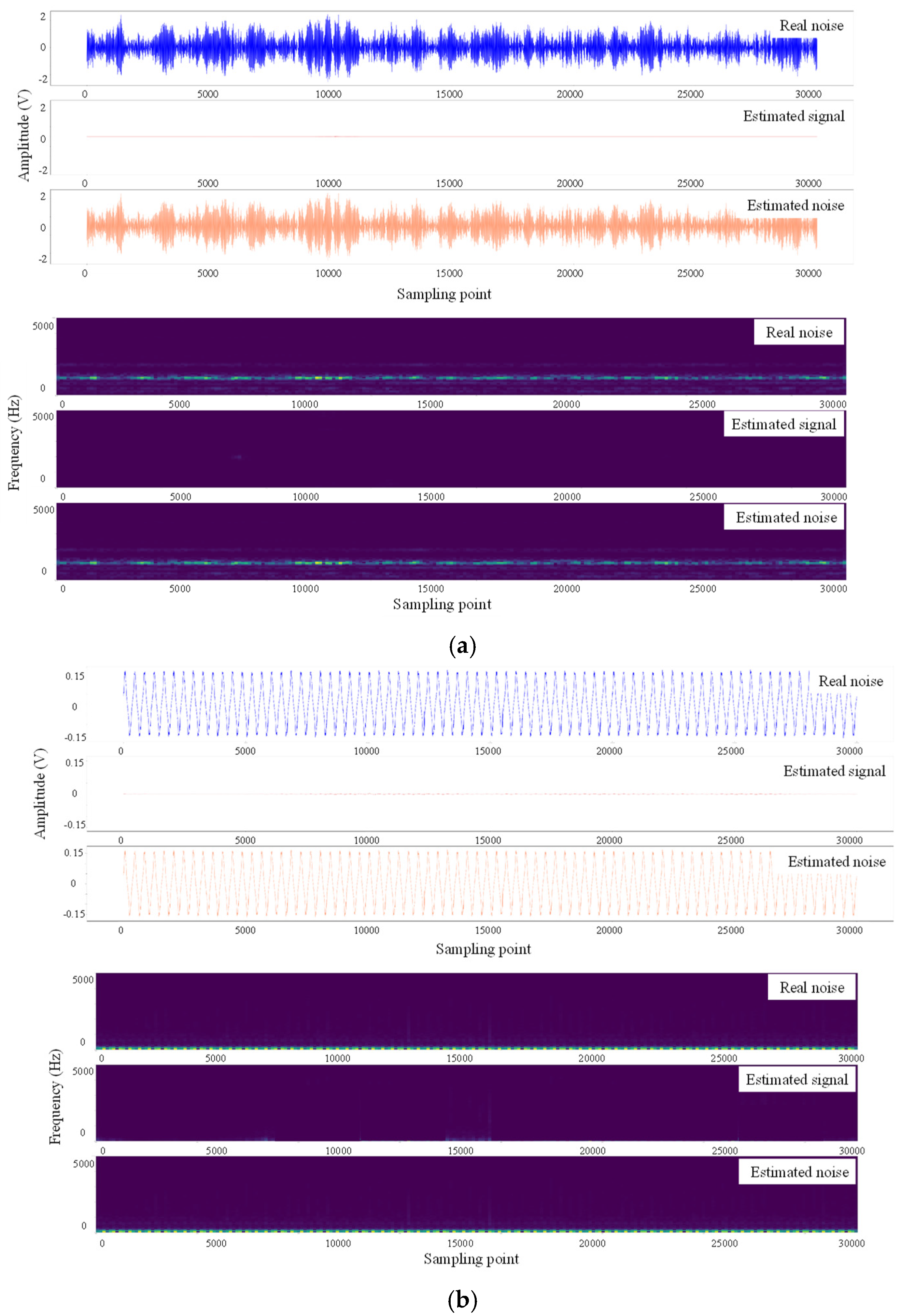
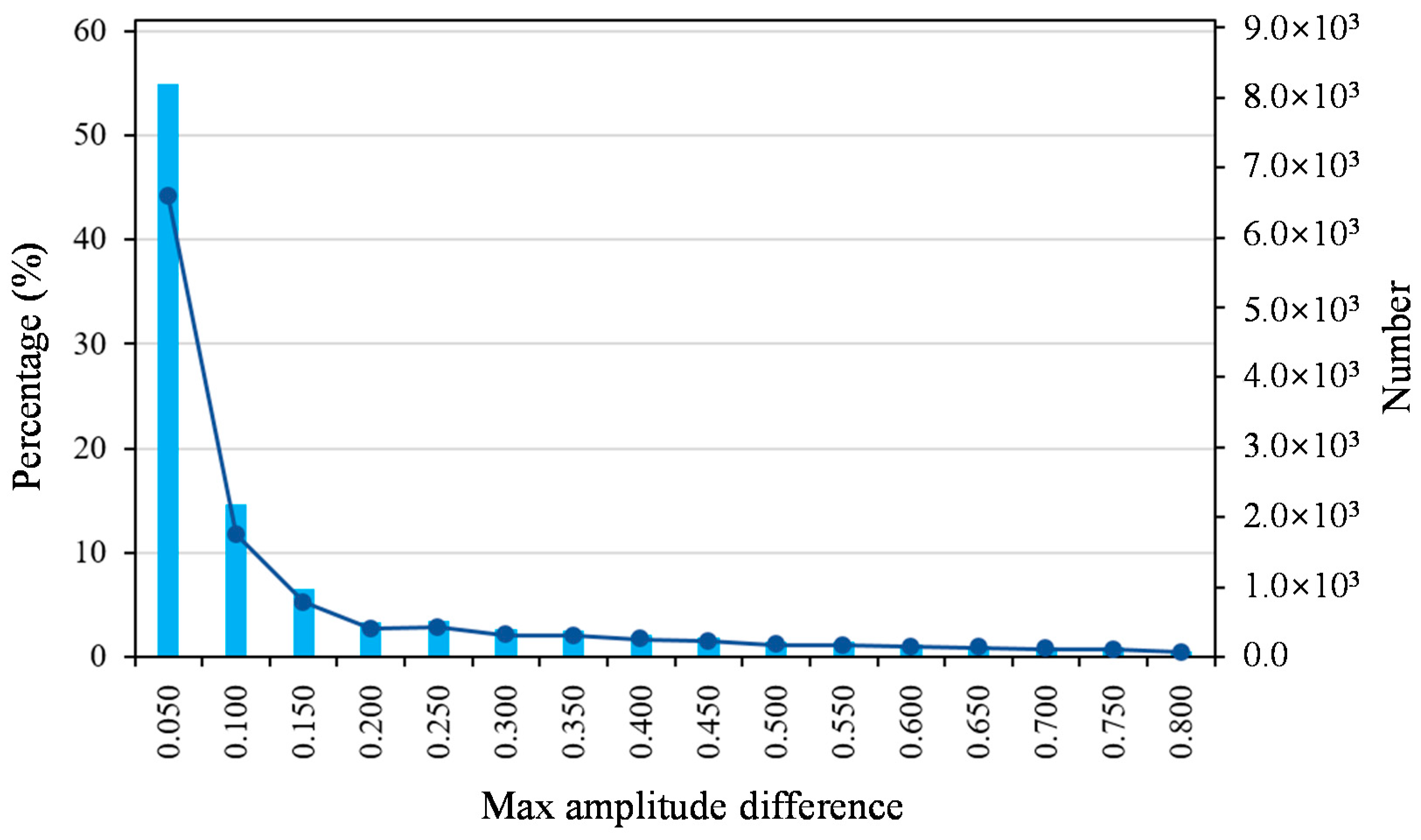
The proposed model not only learns the features of microseismic signals but also estimates noise. To validate this, the CNN-denoiser was tested for 12,000 real noise samples. Figure 4 shows the robustness of the neural network to some periodic non-microseismic signals (the frequency band varying with time). No estimated signals are predicted, and the estimated noise is almost equivalent to the input noise sample. It indicates that the CNN-denoiser can automatically produce a mask that adapts to the noise characteristics. The mask reflects the changes in frequency characteristics over time, as well as the frequency band of noise. Additionally, the distribution of the max amplitude difference between the real and estimated noise samples is shown in Figure 5. The results show that the max amplitude difference of more than 50% of noise samples is less than 0.05, which means the method only causes minor waveform distortion.
3.2. Application in Real Field
To validate the versatility, the CNN-denoiser was also applied to the 1510 noisy signals recorded in Zijing tunnel. These noisy signals include various types and intensities of noise so that the SNRs ranged from 0 to 15 dB (Figure 6). SNR [28] is calculated as follows:
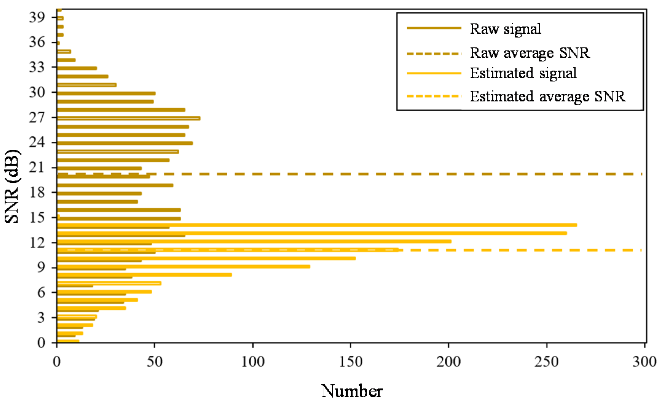
where and are peak amplitudes of signal and noise, respectively. As shown in Figure 6, the proposed method provides an excellent denoising performance for microseismic signals with various noise in terms of the improvement of the SNRs, good shape recovery, and amplitude characteristics, even one noisy signal contains more than one microseismic waveform (Figure 6d). The average SNR of the 1510 noisy signals after denoising is increased by 8.48 dB, and the maximum improvement up to 36.21 dB (Figure 7). In addition, the shape and amplitude characteristics of the estimated noise are well preserved. Although the CNN-denoiser is trained on semi-synthetic data, it could well be extended to real noisy signals. This suggests that the proposed method in this study can be directly applied to actual engineering for denoising tasks.
4. Comparison with Other Existing Methods
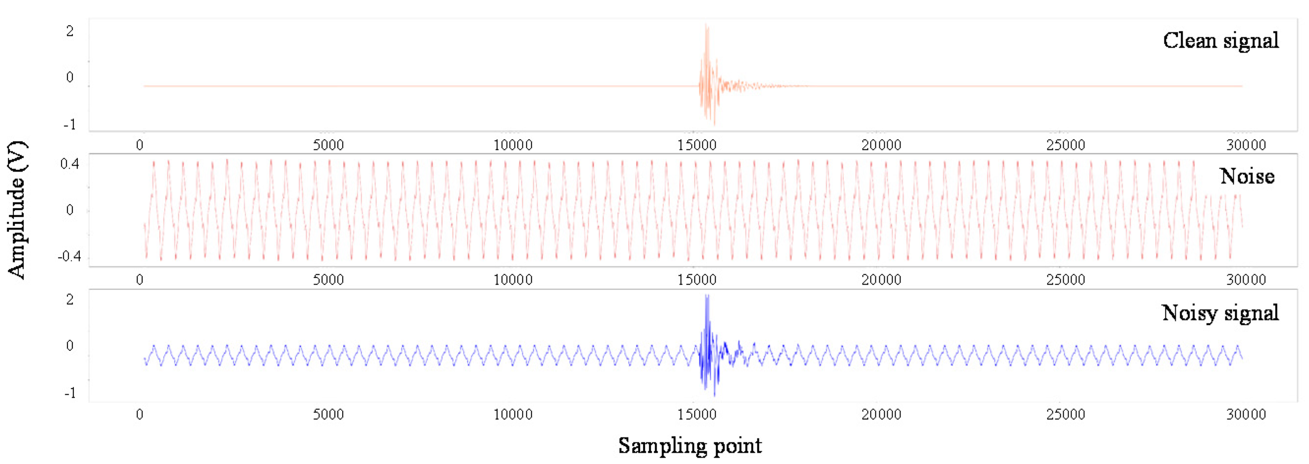
To further demonstrate the denoising performance, the proposed method is compared with other existing methods on a benchmark that is constructed by combining one clean microseismic waveform and one noise. As shown in Figure 8, the amplitude of the noise is varied for different SNRs.
The proposed CNN-denoiser is compared to the high-pass filter and wavelet threshold (WT) filter on the performance of signal denoising. The high-pass filter was designed based on the frequency distribution of clean microseismic signals and noise to achieve the best performance of denoising. In WT filter, the wavelet base of Sym8 was selected, and the seven layers of decomposition and domain value were fixed; the soft threshold was used for microseismic signal denoising. Four measures were employed to compare the methods: the improvements of SNRs between noisy signals and estimated microseismic signals, the correlation coefficient, the changes of the maximum amplitude, and the errors of onset time picking. The Short Term Averaging/Long Term Averaging (STA/LTA) methods for onset time picking was used, and the threshold of the STA/LTA method was set to maximize the accuracy of the onset time picking.
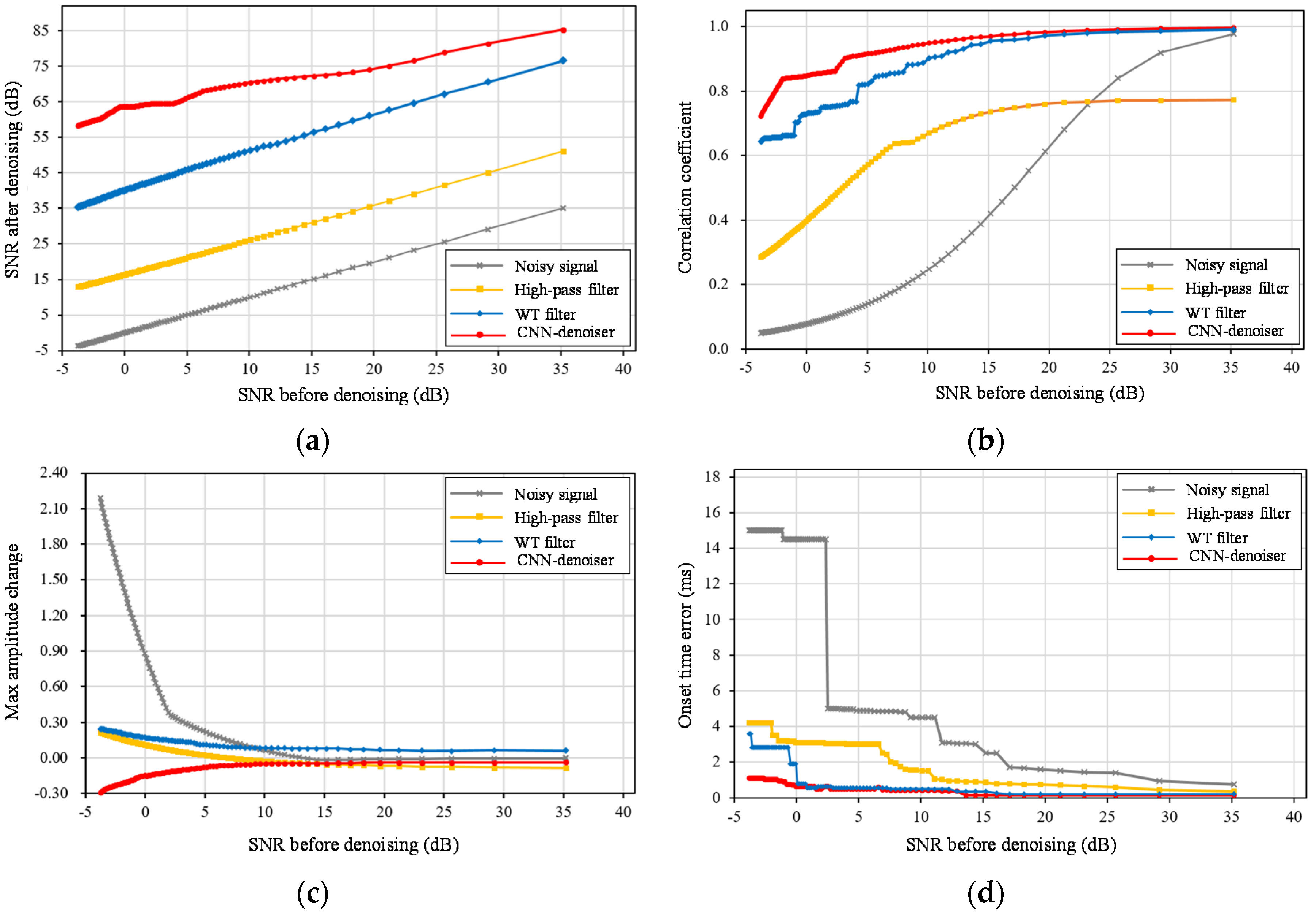
Compared with the high-pass filter and WT filter, the proposed CNN-denoiser outperforms SNR improvements with a maximum of 64.85 dB (Figure 9a). The highest correlation coefficient of estimated signals indicates that the WT filter and CNN-denoiser causes smaller waveform distortion during denoising, and the performance of the latter is better than the former. In contrast, the high-pass filter method introduces high waveform distortion, so that the maximum correlation coefficient only reached 0.86 (Figure 9b). CNN-denoiser provides the highest correction coefficient, especially for low SNRs. Figure 9c shows that the absolute value of max amplitude changes of the estimated signals by the high-pass filter and CNN-denoiser are almost similar when the SNR is less than 10 dB. However, the CNN-denoiser is superior to the high-pass filter in terms of the max amplitude changes of noisy signals with high SNRs, indicating that the max amplitude of the estimated signal is closer to the clean signal in Figure 8. Moreover, the max amplitude change caused by the WT filter is the largest in the test. The STA/LTA method is applied to pick up the onset time of the noisy signal and that denoised by the high-pass filter, WT filter, and CNN-denoiser. As shown in Figure 9d, the accuracy of the onset time picking is significantly improved with the high-pass filter, WT filter and the CNN-denoiser, where the CNN-denoiser outperforms the others for low SRNs. It represents an improvement compared with the STA/LTA methods.
Although the semi-synthetic data are used for training the network, the performance of the CNN-denoiser on microseismic signal denoising shows its robustness by maintaining an optimal accuracy. However, for new complex noise or microseismic signal samples, the method may not achieve the current performance, which needs validation in further research. The current estimation of the microseismic signal is based on the output of masks, and thus non-mask prediction will be the direction of future research [29]. The increase in training data can continuously separate the microseismic signal and noise perfectly, which will be the goal of the future research. Further, the combination of traditional methods and the neural network will be explored.
5. Conclusions
In this paper, an advanced processing method for microseismic signals (CNN-denoiser) based on the deep neural network is proposed. The performance of the proposed method outperforms the microseismic signals corrupted with various types and intensities of noise for denoising, even when the frequency bands of microseismic signal and noise overlap. The signal and noise components in the data are appropriately recognized and separated, even if the signal is heavily polluted by noise. The results show that the proposed method significantly improves the SNRs with minor changes of the microseismic signal, and also preserves the shape and amplitude characteristics are well. Moreover, generalization ability was validated on the other dataset outside of the training dataset. Compared with existing methods, the CNN-denoiser significantly improves the SNRs and introduces less distortion in the waveform which allows better recovery of the real waveform. Although the motivation of this study is the need for accurate and automated microseismic signal processing, the proposed method can be applied for signal analysis and disaster assessment in geophysical and geotechnical engineering fields, such as hydraulic fracturing, the mining industry, shale-gas exploitation, and earthquake management.
Author Contributions
Writing—original draft preparation, H.Z.; writing—review and editing, C.M., V.P. and Y.Z.; supervision, N.C.; funding acquisition, C.M. All authors have read and agreed to the published version of the manuscript.
Funding
This work was financially supported by the National Natural Science Foundation of China (grant numbers 41807255); State Key Laboratory of Geohazard Prevention and Geoenvironment Protection Independent Research Project (grant number SKLGP2018Z016); Sichuan Science and Technology Project (grant number 2019YJ0465).
Conflicts of Interest
The authors declare no conflict of interest.
References
- Douglas, A. Bandpass filtering to reduce noise on seismograms: Is there a better way? Bull. Seismol. Soc. Am. 1997, 87, 770–777. [Google Scholar]
- Scherbaum, F. Of Poles and Zeros: Fundamentals of Digital Seismology; Kluwer Academic Publishers: Berlin, Germany, 2001. [Google Scholar]
- Allen, J.B.; Rabiner, L.R. A unified approach to short-time Fourier analysis and synthesis. Proc. IEEE 1977, 65, 1558–1564. [Google Scholar] [CrossRef]
- Mousavi, S.M.; Langston, C.A. Hybrid seismic denoising using higher-order statistics and improved wavelet block thresholding. Bull. Seismol. Soc. Am. 2016, 106, 1380–1393. [Google Scholar] [CrossRef]
- Mousavi, S.M.; Langston, C.A. Adaptive noise estimation and suppression for improving microseismic event detection. J. Appl. Geophys. 2016, 32, 116–124. [Google Scholar] [CrossRef]
- Tselentis, G.A.; Martakis, N.; Paraskevopoulos, P.; Lois, A.; Sokos, E. Strategy for automated analysis of passive microseismic data based on s-transform, Otsu’s thresholding, and higher order statistics. Geophysics 2012, 77, KS43–KS54. [Google Scholar] [CrossRef] [Green Version]
- Sabbione, J.I.; Sacchi, M.D.; Velis, D.R. Microseismic Data Denoising via an Apex-Shifted Hyperbolic Radon Transform. Available online: https://library.seg.org/doi/abs/10.1190/segam2013-1414.1 (accessed on 22 September 2020).
- Sabbione, J.I.; Sacchi, M.D.; Velis, D.R. Radon transform-based microseismic event detection and signal-to-noise ratio enhancement. J. Appl. Geophys. 2015, 113, 51–63. [Google Scholar] [CrossRef]
- Zhang, L.; Wang, Y.; Zheng, Y.; Chang, X. Deblending using a high-resolution radon transform in a common midpoint domain. J. Geophys. Eng. 2015, 12, 167–174. [Google Scholar] [CrossRef]
- Galiana-Merino, J.J.; Rosa-Herranz, J.; Giner, J.; Molina, S.; Botella, F. De-noising of short-period seismograms by wavelet packet transform. Bull. Seismol. Soc. Am. 2003, 93, 2554–2562. [Google Scholar] [CrossRef]
- Liu, S.C.; Chen, X. Seismic signals wavelet packet denoising method based on improved threshold function and adaptive threshold. Comput. Model. New Tech. 2014, 18, 1291–1296. [Google Scholar]
- Huang, N.E.; Shen, Z.; Long, S.R.; Wu, M.C.; Shi, H.H.; Zheng, Q.; Yen, N.C.; Tung, C.C.; Liu, H.H. The empirical mode decomposition and the Hilbert spectrum for nonlinear and non-stationary time series analysis. Proc. Roy. Soc. A-Math. Phy. 1998, 454, 903–995. [Google Scholar] [CrossRef]
- Chen, W.; Xie, J.Y.; Zu, S.H.; Gan, S.W.; Chen, Y.K. Multiple-reflection noise attenuation using adaptive randomized-order empirical mode decomposition. IEEE Geosci. Remote Sens. Lett. 2017, 14, 18–22. [Google Scholar] [CrossRef]
- Bekara, M.; Baan, M.V.D. Random and coherent noise attenuation by empirical mode decomposition. Geophysics 2009, 74, 89–98. [Google Scholar] [CrossRef]
- Hashemi, H.; Javaherian, A.; Babuska, R. A semi-supervised method to detect seismic randomnoise with fuzzy GK clustering. J. Geophys. Eng. 2008, 5, 457–468. [Google Scholar] [CrossRef]
- Oropeza, V.; Sacchi, M. Simultaneous seismic data denoising and reconstruction via multichannel singular spectrum analysis. Geophysics 2011, 76, V25–V32. [Google Scholar] [CrossRef]
- Chen, Y.; Ma, J.; Fomel, S. Double-sparsity dictionary for seismic noise attenuation. Geophysics 2016, 81, V17–V30. [Google Scholar] [CrossRef]
- Li, H.; Wang, R.; Cao, S.; Chen, Y.; Huang, W. A method for low frequency noise suppression based on mathematical morphology in microseismic monitoring. Geophysics 2016, 81, V159–V167. [Google Scholar] [CrossRef]
- Bonar, D.; Sacchi, M. Denoising seismic data using the nonlocal means algorithm. Geophysics 2012, 77, A5–A8. [Google Scholar] [CrossRef]
- Rao, Y.Z.; Wang, L.; Rao, R.; Shao, Y.J.; Liu, J. A method for blasting vibration signal denoising based on empircal mode decomposition and wavelet threshold. J. Fuzhou Univ. (Nat. Sci. Ed.) 2015, 43, 271–277. [Google Scholar]
- Goodfellow, I.; Bengio, Y.; Courville, A. Deep Learning; MIT Press: Cambridge, MA, USA; London, UK, 2016; Volume 1. [Google Scholar]
- Perol, T.; Gharbi, M.; Denolle, M. Convolutional neural network for earthquake detection and location. Sci. Adv. 2018, 4, e1700578. [Google Scholar] [CrossRef] [Green Version]
- Ross, Z.E.; Meier, M.A.; Hauksson, E. P-wave arrival picking and first-motion polarity determination with deep learning. J. Geophys. Res. Solid Earth 2018, 123, 5120–5129. [Google Scholar] [CrossRef]
- Zheng, J.; Lu, J.; Peng, S.; Jiang, T. An automatic microseismic or acoustic emission arrival identification scheme with deep recurrent neural networks. Geophys. J. Int. 2018, 212, 1389–1397. [Google Scholar] [CrossRef]
- Zhu, W.Q.; Beroza, G.C. Phasenet: A deep-neuralnetwork-based seismic arrival time picking method. Geophys. J. Int. 2018, 216, 261–273. [Google Scholar] [CrossRef] [Green Version]
- Ioffe, S.; Szegedy, C. Batch Normalization: Accelerating Deep Network Training by Reducing Internal Covariate Shift. In Proceedings of the 32nd International Conference on Machine Learning, Lile, France, 7–9 July 2015; pp. 448–456. [Google Scholar]
- Ronneberger, O.; Fischer, P.; Brox, T. U-Net: Convolutional Networks for Biomedical Image Segmentation. In Medical Image Computing and Computer-Assisted Intervention—MICCAI 2015; Navab, N., Hornegger, J., Wells, W., Frangi, A., Eds.; Lecture Notes in Computer Science; Springer: Cham, Switzerland, 2015. [Google Scholar]
- Mousavi, S.M.; Zhu, W.Q.; Sheng, Y.X.; Beroza, G.C. Cred: A deep residual network of convolutional and recurrent units for earthquake signal detection. Sci. Rep. 2019, 9, 10267. [Google Scholar] [CrossRef] [PubMed]
- Zhu, W.Q.; Mousavi, S.M.; Beroza, G.C. Seismic Signal Denoising and Decomposition Using Deep Neural Networks. IEEE Trans. Geosci. Remote Sens. 2019, 57, 9476–9488. [Google Scholar] [CrossRef] [Green Version]
- Mantovani, E.; Albarello, D.; Mucciarelli, M. Seismic activity in North Aegean Region as middle-term precursor of Calabrian earthquakes. Phys. Earth Planet. Int. 1986, 44, 264–273. [Google Scholar] [CrossRef]
Figure 1.
The neural network structure of the proposed convolutional neural network (CNN)-denoiser. Inputs are the real and imaginary parts of time–frequency coefficients of the noisy signal. The gray rectangles represent the neural network layers. Arrows represent different operations applied between two adjacent layers. Batch normalization and concatenate are used to improve convergence during training. The dimension of each layer presented above indicates “frequency bins × time points × filters”. Outputs are two masks for the estimation of the time–frequency coefficients of the microseismic signal and noise.

Figure 2.
Flow diagram of the method. ① The noisy signal is transformed from the time domain into the time–frequency domain using Short Time Fourier Transform (STFT). ② The real and imaginary parts of time–frequency coefficients of noisy signals are input into the neural network. ③ Two masks from the network are applied to the real and imaginary parts of time–frequency coefficients of the input noisy signal to estimate the time–frequency coefficients of microseismic signal and noise, respectively. ④ The estimated signal and noise in the time domain are obtained via the inverse STFT.

Figure 3.
Denoising performance of CNN-denoiser for noisy signals with various noise in the test dataset. The signals in the time domain and time–frequency domain for each sub-figure are clean signal, real noise, noisy signal, estimated signal, and estimated noise from top to bottom. (a,b) Microseismic signals with cyclic noises at different frequency; (c) microseismic signals with a mixture of cyclic noise and other noise; (d) microseismic signals with Gaussian noise.


Figure 4.
Denoising performance of CNN-denoiser for different types of real noise. The noises in the time domain and time–frequency domain are real noise, estimated signal and estimated noise from top to bottom of each sub-figure. (a) Mixture of cyclic noise and other noise; (b) cyclic noise.
Figure 4.
Denoising performance of CNN-denoiser for different types of real noise. The noises in the time domain and time–frequency domain are real noise, estimated signal and estimated noise from top to bottom of each sub-figure. (a) Mixture of cyclic noise and other noise; (b) cyclic noise.

Figure 5.
Distribution of max amplitude difference between real and estimated noise.

Figure 6.
Denoising examples of different recorded noisy signals in Zijing tunnel (China). The signals in the time domain and time–frequency domain are noisy signal, estimated signal, and estimated noise from top to bottom of each sub-figure. (a,b) Microseismic signals with cyclic noises at different frequency; (c) microseismic signal with a mixture of cyclic noise and other noise; (d) noisy signal contains more than one microseismic waveform.


Figure 7.
Signal-to-noise ratio (SNR) distribution of noisy signals before and after denoising by CNN-denoiser in Zijing tunnel (China).
Figure 7.
Signal-to-noise ratio (SNR) distribution of noisy signals before and after denoising by CNN-denoiser in Zijing tunnel (China).

Figure 8.
The noisy signal was formed by superimposing the clean signal with noise. Clean signal and noise were all recorded by the same microseismic monitoring acquisition station in Micang Mountain tunnel (China).
Figure 8.
The noisy signal was formed by superimposing the clean signal with noise. Clean signal and noise were all recorded by the same microseismic monitoring acquisition station in Micang Mountain tunnel (China).

Figure 9.
Performance comparison between high-pass filter, wavelet threshold (WT) filter and CNN-denoiser. (a–c) Improvement of SNRs, correlation coefficient, and max amplitude changes between the high-pass filter, WT filter and CNN-denoiser. (d) The error of onset time picking by Short Term Averaging/Long Term Averaging (STA/LTA) (applied to noisy signal and that denoised by a high-pass filter, WT filter and CNN-denoiser). Values in (b) are calculated by Pearson product-moment correlation coefficient [30] between the estimated signals (noisy signal and that denoised by a high-pass filter, WT filter and CNN-denoiser) and the clean signal in Figure 8. Values in (c) and (d) are differences between the estimated signals (noisy signal and that denoised by a high-pass filter, WT filter and CNN-denoiser) and the clean signal in Figure 8.

© 2020 by the authors. Licensee MDPI, Basel, Switzerland. This article is an open access article distributed under the terms and conditions of the Creative Commons Attribution (CC BY) license (http://creativecommons.org/licenses/by/4.0/).
Share and Cite
MDPI and ACS Style
Zhang, H.; Ma, C.; Pazzi, V.; Zou, Y.; Casagli, N. Microseismic Signal Denoising and Separation Based on Fully Convolutional Encoder–Decoder Network. Appl. Sci. 2020, 10, 6621. https://0-doi-org.brum.beds.ac.uk/10.3390/app10186621
AMA Style
Zhang H, Ma C, Pazzi V, Zou Y, Casagli N. Microseismic Signal Denoising and Separation Based on Fully Convolutional Encoder–Decoder Network. Applied Sciences. 2020; 10(18):6621. https://0-doi-org.brum.beds.ac.uk/10.3390/app10186621
Chicago/Turabian StyleZhang, Hang, Chunchi Ma, Veronica Pazzi, Yulin Zou, and Nicola Casagli. 2020. "Microseismic Signal Denoising and Separation Based on Fully Convolutional Encoder–Decoder Network" Applied Sciences 10, no. 18: 6621. https://0-doi-org.brum.beds.ac.uk/10.3390/app10186621
Note that from the first issue of 2016, this journal uses article numbers instead of page numbers. See further details here.