A Machine Learning Framework for Assessing Seismic Hazard Safety of Reinforced Concrete Buildings

Abstract

Although averting a seismic disturbance and its physical, social, and economic disruption is practically impossible, using the advancements in computational science and numerical modeling shall equip humanity to predict its severity, understand the outcomes, and equip for post-disaster management. Many buildings exist amidst the developed metropolitan areas, which are senile and still in service. These buildings were also designed before establishing national seismic codes or without the introduction of construction regulations. In that case, risk reduction is significant for developing alternatives and designing suitable models to enhance the existing structure’s performance. Such models will be able to classify risks and casualties related to possible earthquakes through emergency preparation. Thus, it is crucial to recognize structures that are susceptible to earthquake vibrations and need to be prioritized for retrofitting. However, each building’s behavior under seismic actions cannot be studied through performing structural analysis, as it might be unrealistic because of the rigorous computations, long period, and substantial expenditure. Therefore, it calls for a simple, reliable, and accurate process known as Rapid Visual Screening (RVS), which serves as a primary screening platform, including an optimum number of seismic parameters and predetermined performance damage conditions for structures. In this study, the damage classification technique was studied, and the efficacy of the Machine Learning (ML) method in damage prediction via a Support Vector Machine (SVM) model was explored. The ML model is trained and tested separately on damage data from four different earthquakes, namely Ecuador, Haiti, Nepal, and South Korea. Each dataset consists of varying numbers of input data and eight performance modifiers. Based on the study and the results, the ML model using SVM classifies the given input data into the belonging classes and accomplishes the performance on hazard safety evaluation of buildings.

1. Introduction

A structure’s seismic vulnerability is a quantity correlated with its failure in the event of earthquakes of previously known intensity. This quantity and seismic hazard experience’s importance helps us determine the potential risk from future earthquakes [1]. Many destructive seismic activities have caused immense disruption in human history, resulting in substantial loss of life, severe economic consequences, and severe property damage. There has been a remarkable increase in working personnel’s migration from rural to urban metropolitan regions due to career prospects and lifestyle. As a consequence, this imparts the responsibility of protecting the high occupancy of urban infrastructure. Old buildings still in service, historical structures with heritage, high importance buildings, and buildings not compliant with the latest seismic codes are the buildings with the highest seismic vulnerability. This proves the necessity of manifesting a seismic structural prioritization scheme, which shall prevent damage or adapt to post-disaster management regulations. Rapid Visual Screening (RVS) is a rapid and reliable method for determining the damage index for various buildings [2,3]. Sinha and Goyal [4] have a laconic discussion as motivation for a layman. The United States first recognized the demand for a fast, reliable, and computationally easy method; therefore, the first RVS method was mentioned in 1988 as “Rapid Visual Screening of Buildings for Potential Seismic Hazards: A Handbook” [5]. This RVS approach (1988) was subsequently updated in 2002 with new developments in seismic engineering. However, an in-depth study and detailed analysis bring challenges in the urban sector where buildings are complex and built on the absence of non-standard norms of safety. The research focuses on one of the latest techniques for enhanced vulnerability assessment of reinforced structures. Eventually, many other countries followed this strategy by changing their RVS approaches concerning their local circumstances, improvements, etc. [6]; for instance, Indian RVS (IITK-GSDMA) [7] or the Philippine RVS [8].

The approach of RVS usually begins with a walk down evaluation to perform a visual inspection physically for recording the seismic parameters. For this purpose, the collection of datasheets needs an evaluator. RVS is a highly effective mechanism to prioritize the structures with high vulnerability due to the faster computational time and non-tedious methodology, thereby helping analyze more massive building stock in a short time. The RVS method is based on a scoring system, wherein the final performance score shall be obtained by performing elementary computations. Every singular approach has the respective cut-off score predefined, for instance, the Federal Emergency Management Agency (FEMA). The structures that do not reach the cut-off score shall be subjected to comprehensive second and third assessment stages. We shall note that seismic vulnerability assessment is performed mainly in three stages [9]: walk down an evaluation, preliminary evaluation, and detailed evaluation. The first stage is defined by a physical walk down evaluation with fundamental computations for the screening of vulnerable structures. Structures that struggle to fulfill expectations at this stage will be addressed with further action. The second step consists of a comprehensive analysis conducted by the detailed study of several structure components, such as the actual ground conditions, the quality of the material used, the state of the structural elements, etc. The third stage is brought into action when the structures require a more detailed analysis. The concept of structural activity in seismic activities, defined as non-linear dynamic structural research, is performed here [10].

A substantial literature has been published in the attempts of integrating several methods from various domains with RVS, for instance, statistical methods [11,12], Artificial Neural Network (ANN) [13,14,15,16,17], multi-criteria decision making [18,19], and type-1 [20,21,22,23] and type-2 [24,25] fuzzy logic systems are frequently assimilated within RVS for increasing the interface and efficacy of seismic vulnerability screening. However, there are methods developed to evaluate the damage and change detection of buildings by remote sensing and image analysis [26,27]. The parameter significance and the selection of the optimum number of parameters have been used effectively by Morfidis and Kostinakis [28]. Multiple linear regression analysis [11] is the most commonly used statistical technique for the classification of damage state in the RVS domain, preceded by other approaches, such as discriminant analysis suggested in [29]. Tesfamariam and Liu [15] have effectively applied and utilized eight different statistical risk classification methods, including six-building output modifications (predictor variables) with damage states as none (O), light (L), moderate (M), severe (S), and collapse (C). Furthermore, Jain et al. have proved the integrated use of various exciting variable selection techniques such as R${}^2$ adjusted, forward selection, backward elimination, and Akaike’s and Bayesian information criteria [30]. Besides, the traditional least square regression analysis and multivariable linear regression analysis were used in the research proposed in [31]. Several probabilistic models are suggested, such as reliability-based models and “best estimate” matrices of the potential damage [32].

Morfidis and Kostinakis [33] have proposed a unique and innovative ANN application from a practical perspective. The coupling of fuzzy logic and ANN’s has been used in a study by Dristos [34], where untrained fuzzy logic procedures are remarkable. Nevertheless, several of the previous RVS approaches are based on the expert’s view, complexities, or conclusions in the linear parameter relationship. Machine Learning (ML), an artificial intelligence division, uses computational algorithms capable of automatic creation by training and learning. This focuses on rendering the forecasts using data analysis software. The ML algorithms generally comprise of three fundamental components: representation, evaluation, and optimization. A method known as Support Vector Machine (SVM) has been commonly used in scenarios of processing uncertain data or data without necessary records that need to be processed efficiently. SVM performs adequately even for the provided information in the context of unstructured and semi-structured data, such as tests of images merged with trees. Kernel trick is one of SVM’s strengths that integrates all the knowledge required for the learning algorithm to identify a core object in the transformed field [35]. The implementation of SVM with initially supervised learning data-sets is seen in this analysis. The damage records of 4 different earthquakes have been taken to implement from countries such as Ecuador, Haiti, Nepal, and South Korea. Finally, the work demonstrates the SVM model’s expertise and the detailed interpretation of the chosen earthquakes result.

2. Background of the Selected Earthquakes

In this study, the archived data of buildings on the open-access database on the Datacenterhub platform [36] were used. These buildings were affected during Nepal, Haiti, South Korea, and Ecuador earthquakes, and they were investigated further by different research groups, and their information and observed damage were collected.

The entire province across Ecuador is prone to seismic hazards, and in this study, one of the current earthquakes, which occurred on 16 April 2016, and majorly affected the coastal zone of Manabí, has been selected. The data collection has been carried through the American Concrete Institute (ACI) research team to generate a memorandum of damaged RC structures affected due to the earthquake. These teams collaborated with the technical staff and students of the Escuela Superior Politécnica del Litoral (ESPOL) [37]. The data have two different soil profiles known as APO1 (the location of the IGN strong-motion station) and Los Tamarindos. APO1 is situated amid alluvial soils and colluvial deposits with an average shear wave velocity at the height of 30 m, Vs30 of 240 m/s, whereas Los Tamarindos is within the alluvial clay and silt deposits with, Vs30 of 220 m/s [38].

Secondly, the Haiti earthquake that occurred on 12 January 2010, has been taken for the assessment. The seismologists have compiled the structural data of 145 RC frames from the University of Purdue, Washington University, and Kansas University have been worked together with research workers from Université d’Etat d’Haïti [39,40]. Soil properties of the data are classified as the granular alluvial fans and the soft clay soils for the southern and the northern plain of Léogâne city, respectively, which is located to the west of Port-au-Prince with the severe structural damage [41]. According to the Shake-Map of the U.S. Geological Survey, Léogâne has a ground motion with the highest instrumental intensity of IX, and Port-au-Prince has intensity VIII [42].

The devastating earthquake which had struck Nepal in May 2015 has also been assessed in the current study. Researchers from the Purdue University and Nagoya Institute of Technology, in association to the ACI, conducted surveys and inspected damaged RC structures. A dataset compilation has been completed in the reconnaissance survey, which has 135 low-rise reinforced concrete buildings with or without masonry infill walls [43]. The fill sediments of the Kathmandu valley’s soil profile mostly consist of a heterogeneous mixture of clays, sands, and silts, which have a thickness of nearly 400 m [44]. Based on the records of the ShakeMap of the U.S. Geological Survey, the ground motion intensity of VIII with the epicenter of 19 KM to the south-east of Kodari.

Ultimately, the earthquake emerged on 15 November 2017, in the Korean territory. Two mega cities Heunghae and Pohang, were influenced by the earthquake event, and due to that, structures were considerably damaged in the vicinity of these areas. Additionally, thousands of inhabitants were homeless caused by severe structural damage, leading to a significant impact on the economy of around 100 million dollars in public and private infrastructures. The collection of damage data had been carried by a team of researchers from ACI in collaboration with multiple universities and research institutes [45].

The subsurface soil strata consist of filling, alluvial soil, weathered soil, weathered rock, and bedrock. The ShakeMap of the U.S. Geological Survey has listed the earthquake intensity as VII [46].

Table 1. Properties of the selected earthquakes.

Earthquake	Year	Moment Magnitude (${\mathit{M}}_{\mathit{w}}$)	PGA (g)	PGV (cm/s)
Ecuador [47]	2016	7.8	0.4	82
Haiti [39]	2010	7	0.4	40
Nepal [48]	2015	7.3	0.2	20
S. Korea [49]	2017	5.4	0.2	10

indicates the details of selected earthquakes and related parameters.

Choice of Building’s Damage Inducing Parameters

It is necessary to gather certain primary information beforehand, to begin with, every RVS process. Several experiments have investigated the usefulness of building characteristics as input variables for evaluating seismic susceptibility [18,50,51]. In line with FEMA154 [5], many of the methods as mentioned earlier contained parameters and exhibited that the most useful inputs are namely, (i) system type, (ii) vertical irregularity, (iii) plan irregularity, (iv) year of construction, and (v) quality of construction. Yakut et al. [52] considered more criteria for the seismic risk assessment of buildings. Concerning the characteristics of the affected structures and the tremendous amount of current building stocks, the following eight criteria were formulated for research purposes. The criteria considered are No. of story, total floor area, column area, concrete wall area in X and Y directions, masonry wall area in X and Y directions, and captive columns. These parameters also form the basis of the Priority Index (PI), as proposed by Hasan and Sozen [53]. These parameters have been selected because the effect of these has been examined and adjusted to assess structures, not meeting code requirements. The parameters can also be applied to different regions as they have been tested in areas with different construction practices. Furthermore, the parameters are easily collected by visual inspection, which leads to a lowered vagueness for investigators, thereby saving time. The eight parameters have been presented in

Table 2. Parameters for earthquake hazard safety assessment [16].

Variable	Parameter	Unit	Type
${\alpha }_1$	No. of story	N	Quantitative
${\alpha }_2$	Total Floor Area	${\mathrm{m}}^2$	Quantitative
${\alpha }_3$	Column Area	${\mathrm{m}}^2$	Quantitative
${\alpha }_4$	Concrete Wall Area (Y)	${\mathrm{m}}^2$	Quantitative
${\alpha }_5$	Concrete Wall Area (X)	${\mathrm{m}}^2$	Quantitative
${\alpha }_6$	Masonry Wall Area (Y)	${\mathrm{m}}^2$	Quantitative
${\alpha }_7$	Masonry Wall Area (X)	${\mathrm{m}}^2$	Quantitative
${\alpha }_8$	Captive Columns	N (exist = 1, absent = 0)	Dummy

.

3. ML Approach for Multi-Class Classification

ML classifies objects quite fast and efficiently, which humans may find it difficult to analyze because of complex numbers, vast data, or a huge number of features. ML algorithms are primarily for binary classifications. However, when added to the present algorithms, several techniques allow successfully to segregate the multi-class entity. SVM strongly solves multi-class classification or regression problems for wide assorted fields, like Anomaly Detection, text or image categorization, time-series analysis, and medical informatics [54]. The study has enforced the SVM algorithm on the datasets using techniques like One-vs.-All [55] and GridSearchCV to build an SVM classifier for multi-classes classification efficiently.

Figure 1 presents an approximate procedural used in the study. The workflow comprises data pre-processing, data splitting, model building, model fitting, accuracy optimization, and visualization; each step is elaborated in the following sub-sections.

3.1. Data Pre-Processing

Data are an integral part of any ML classifier, and they are composed of input features as independent variables and labeled output as the dependant variable. The quality of data and the information derived from a dataset influence the learning capacity of the model. Therefore, pre-processing before feeding the data to the model is essential. Row data may contain null values, outliers, and non-categorical data. ML is taught to classify only using categorical data, and it can not process ordinal or numeric datatype. Library “Panda” is well-known in such a situation for data manipulation and analysis. It fits 1 for the input observations that belong to the particular class, leaving the rest of the observation 0. Similar function is performed by One-Hot-Encoding in sklearn library. ML treats missing value as NaN also known as not-a-number. There are several ways to deal with missing data, like omitting the complete row to which the missing value belongs, or replacing the missing value with mean, median, or most occurred observation. SimpleImputer from sklearn easily imputes the missing data with a constant value or using statistics like mean, median, or most common value. Often the dataset accommodates attributes with a mixture of scale. ML models anticipate or are more efficient if the data follow the same scale. Data standardization or normalization are commonly practiced methods for data re-scaling, availed in sklearn. Data standardization is the distribution of attribute between a mean of zero and a standard deviation of one (unit variance), whereas data normalization is scaling of attributes into the range 0 and 1.

3.2. Imbalanced Data

A frequent problem in ML classification is a disproportionate ratio among the number of attributes in each class, called as imbalanced classes [56]. The classifier’s efficiency and accuracy are optimal when an equal number of samples are present for each class. A classification problem may be slightly skewed if there is a small imbalance. On the other hand, classification problems could face significant disagreement if the number of examples is enormous for one class and very few in another class for a given training dataset. Random sampling is a common approach used to address the problem of imbalanced data. Several proven approaches help deal with imbalanced data. Like, Random Under-sampling is a random deletion of excess examples in the majority class, and Random Over-sampling is random duplication of examples in the minority class. Random Under-sampling is not a preferred method when the data are crucial, and discarding or deleting data can cause information loss. SMOTE, i.e., Synthetic Minority Over-sampling Technique from library imblearn works well in most scenarios as it merely adds examples in minority class without adding any new information to the class.

3.3. Classification

Machine Learning is well-known for classification problems, either binary or multi-class classification. Depending on the case study, the selection of the input parameter varies. In general, including a few essential parameters create a better impact in accuracy than a high number of less critical input parameters.

The classification of the buildings’ damage states is ranked to anticipate the risk associated with each structure.

Table 3. Damage classification (adopted from [57]).

Damage Grade	Damage State	Damage Visibility
1	None	No damage
2	Light	Cause hairline cracks in the structure; resigned plasters
3	Moderate	Breaking plasters; teared walls and visible joints between panels
4	Severe	Reduced regional structural and wide wall plans

summarizes the representation of damage states and their associated damage used in the study.

3.4. Splitting of Dataset

Splitting the dataset appears as essential to overcome the bias towards training data in ML algorithms. ML classifiers often overfit the data to fit best the training data, which results in poor prediction performance on actual test data. The training subset creates the predictive model, and the test subset evaluates the performance of the model classifier. As a good practice, 80% of the data goes to the training subset, and 20% falls towards the test subset.

3.5. SVM as Classifier

ML algorithms are broadly classified among supervised learning and unsupervised learning. SVM is a popular supervised learning algorithm and is frequently used to evaluate data for classification and regression analysis. SVM is primarily designed only for two-class distribution [58], but presently the algorithm is advanced and successfully works with multi-class classification problems using kernel tricks [59] and soft margin. This study involves kernel trick with hyperparameter tuning (explained further) for classifying the multi-class building samples to their respective classes. 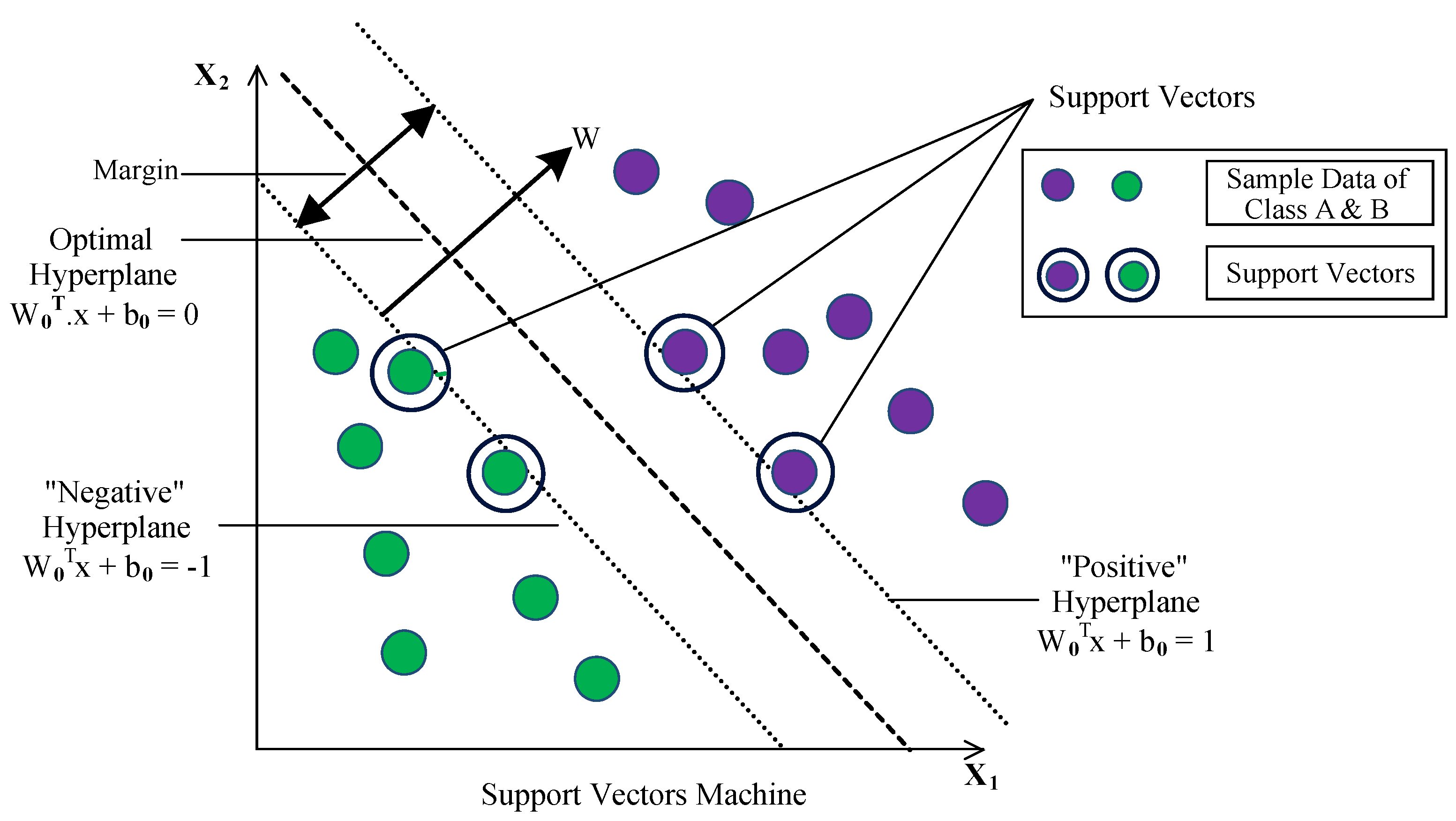Figure 2 shows the elementary SVM classifier mechanism while evaluating two linearly separable classes; for instance, the feature points are considered belonging to the positive class and negative class. SVM takes the feature points and draws the hyperplanes, which separates the points into their belonging classes. An optimal hyperplane or decision boundary is the one that fits best to segregate the feature points. Margin determines the distance of the decision boundary from the nearest data points. Support vectors are the feature points closest to the optimum hyperplane, located at a minimum distance from it.

The hyperplane separating the classes can be represented as [60]:

$${W_0}^{T}x+b_0=y$$

(1)

where, W is the weight to be learn using the training samples,

x denotes the feature vector; $x\in {\mathbb{R}}^n$,

b is a constant,

y is the class value of the training samples; $y\in \{1,-1\}$.

3.6. Performance Evaluation and Utilization of Model

Performance evaluation is an intrinsic part of the classifier modeling process. It finds the optimal classifier representing the sample data and how precisely the built model will perform future data. Performance evaluation of any ML classifier aims to anticipate the prediction accuracy on future or unseen samples. Evaluating the model accuracy with the training set data can overfit the model.

For proper performance interpretation of a model, some part of the dataset is kept on hold as test subset, although the test subset has labeled output. The model gets trained on the training sub-set, and further, the held-out observations are sent to the model to predict. Known labels of the test sub-set are then compared with the prediction returned by the model.

4. Methodology implementation

The study includes data from four different countries, including Ecuador, Haiti, Nepal, and South Korea, with varying numbers of RC building samples, as mentioned earlier from Datacenter hub platform [36,37,40,43,45].

Table 4. Data distribution in the dataset.

Country	Building Samples	Feature Parameters	Damage Classes
Ecuador	171	8	3
Haiti	142	8	3
Nepal	135	8	4
South Korea	67	8	4

presents the distribution of sample data, featured parameter, and damage classes in the given dataset. Each dataset contains eight parameters: number of stories, total floor area, column area, concrete wall area in X and Y direction, masonry wall area in X and Y direction, and captive columns. The damage classes show the severity of the damage caused post the earthquakes.

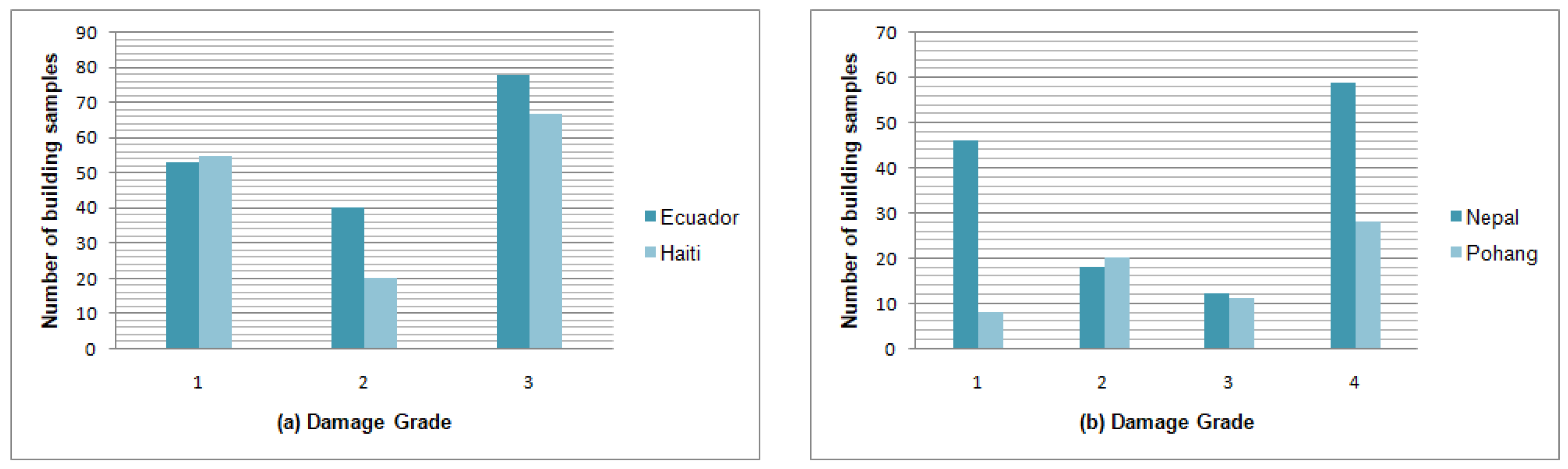
The datasets show an uneven distribution of samples for each damage class. Seismic susceptibility of similar buildings is forecasted based on the relevance damage class. Ecuador and Haiti samples are classified among three different damage classes, whereas Nepal and South Korea samples have four damage classes. The distribution of samples among the damage scales for each dataset is shown in Figure 3.

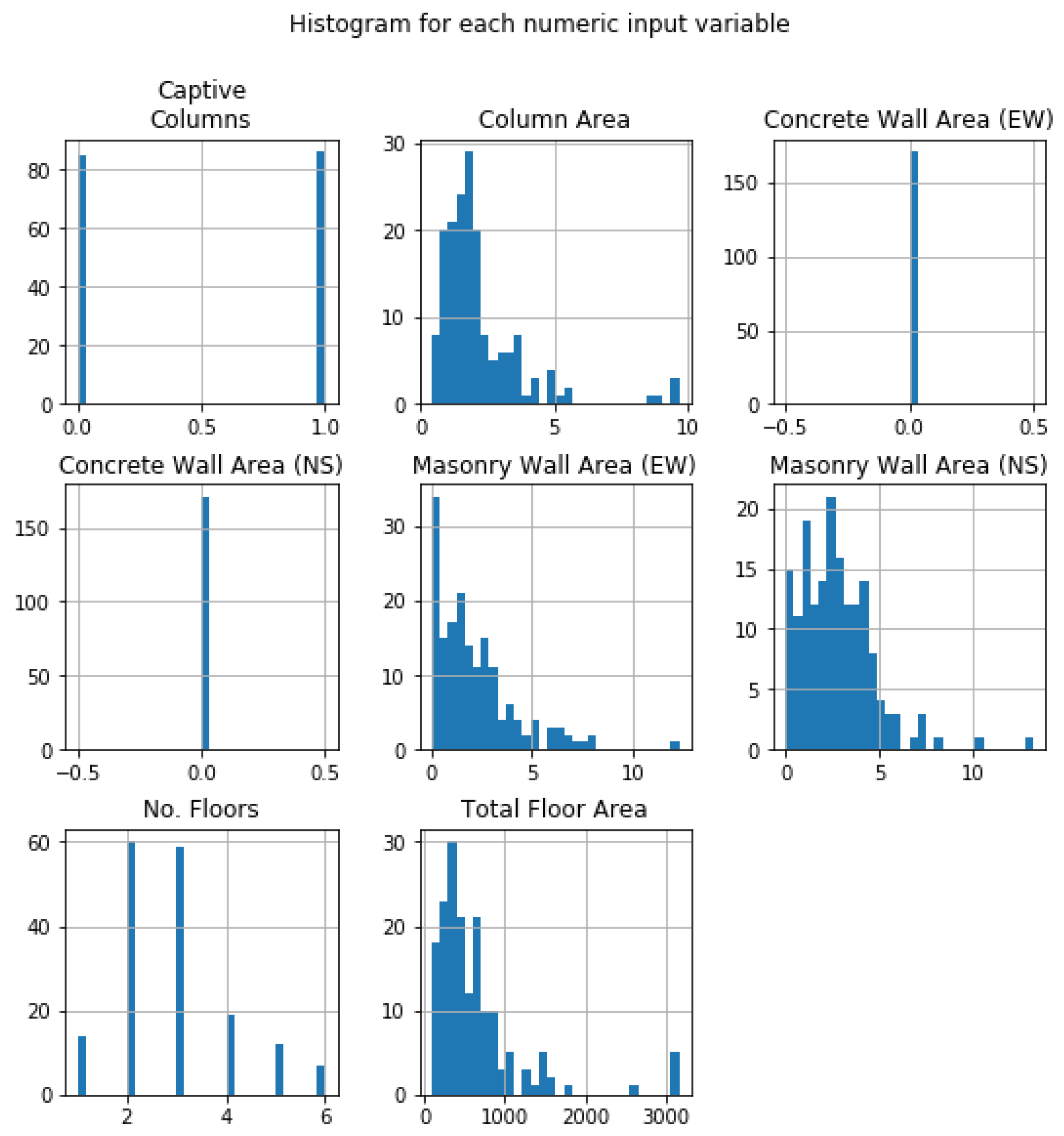
With the histogram’s help, the distribution of data of all the eight parameters within a dataset is assessed. Figure 4 represents the histogram for Ecuador. The abscissa of the plots represents the scale between the highest and the lowest value of each parameter. The frequency distribution of the values shows non-linearity in the variation; rather, column area, Masonry Wall Area (NS), number of floors, and total floor area show Gaussian distribution yet skewed to the left. Masonry wall Area (EW) is distinct from an exponential distribution. Concrete wall area for Y and X directions show no data, while captive columns are distributed bimodally. Haiti, Nepal, and South Korea follow similar non-linear behavior for data distribution.

4.1. Data Pre-Processing

Data pre-processing is critical while feeding the data to the model for learning. There are various ways to manipulate the data as per the requirement; a few important ones are considered for shaping the datasets used in the study.

• Re-scaling the data: To accommodate the data on the same scale, the data are standardized using “MinMaxScaler” from sklearn library. The standardization frames all the input features between 0 and 1, which brings robustness to minimal standard deviation of features and speeds up the algorithm’s calculation.
• Strategy for missing data: The datasets contain very few missing attributes. Removal of data could cause the study of a critical loss of information like the seismic vulnerability test of buildings. Therefore, the missing values are replaced by mean strategy using SimpleImputer from sci-kit learn library.
• Imbalanced data: The imbalanced data in the dataset are handled by Random Over-sampling using SMOTE. It randomly duplicates the minority class’s attributes to match the majority class’s sample number, but do not make any effective change in the class.

  Table 5. Ecuador—Random Over-sampling of data [61].

  Iteration	Class I	Class II	Class III
  0	53	40	78
  1	53	78	78
  2	78	78	78

  ,

  Table 6. Haiti—Random Over-sampling of data [39].

  Iteration	Class I	Class II	Class III
  0	55	20	67
  1	55	67	67
  2	67	67	67

  ,

  Table 7. Nepal—Random Over-sampling of data [62].

  Iteration	Class I	Class II	Class III	Class IV
  0	46	18	12	59
  1	46	18	59	59
  2	46	59	59	59
  3	59	59	59	59

  and

  Table 8. South Korea—Random Over-sampling of data [63].

  Iteration	Class I	Class II	Class III	Class IV
  0	8	20	11	28
  1	28	20	11	28
  2	28	20	28	28
  3	28	28	28	28

  shows how the imbalanced data get manipulate with each iteration for the dataset of Ecuador, Haiti, Nepal, and South Korea, respectively. The final iteration in all datasets has an equal number of data in each class.

4.2. Splitting of Dataset

For all the four datasets, the training and test sub-sets divide into 80% and 20%, respectively. The training set contains all the attributes with labeled output, whereas the test sub-set evaluates the learning performance.

4.3. Hyperparameter Tuning—SVM

While building an ML classifier, there are design choices that define the architecture of the classifier. These choices or parameters are known as hyperparameters, and to achieve an optimal model; the hyperparameters require tuning. Hyperparameters often manage the learning method and the learning pace of the model. Hyperparameters are different from the model parameters, and they can not get trained directly from the data.

SVM has important hyperparameters like kernels, C, and gamma. Kernels modify the training samples to transform any non-linear function into a higher dimension linear function. Radial Basis Function Kernel or RBF, Sigmoid, Polynomial or poly, and Gaussian are few kernel types that SVM uses. Poly and RBF are better suited for multi-class classification problems. Gamma determines the impact of a new feature point on the decision boundary. The high value of gamma means close, and the low value means far from the decision boundary. C acts as a penalty factor for the classifier. Therefore, every time the classifier misclassifies any sample data, the C value increases. Tuning the hyperparameters and finding the optimal accuracy in the model is not cost-effective if processed intuitively. Grid search is reasonably the fundamental tuning approach. Various possible combinations of all hyperparameters are fed into the grid search, and the model architecture with the best accuracy is selected.

5. Result and Discussion

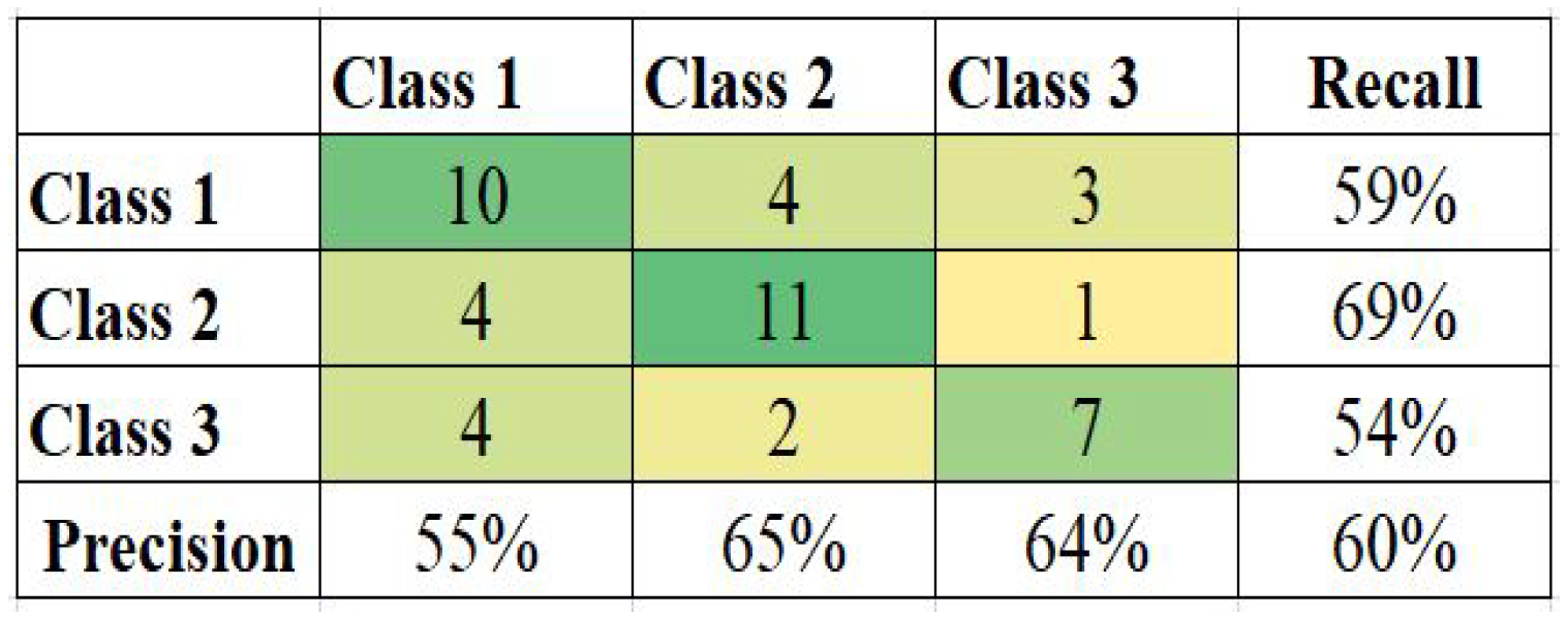
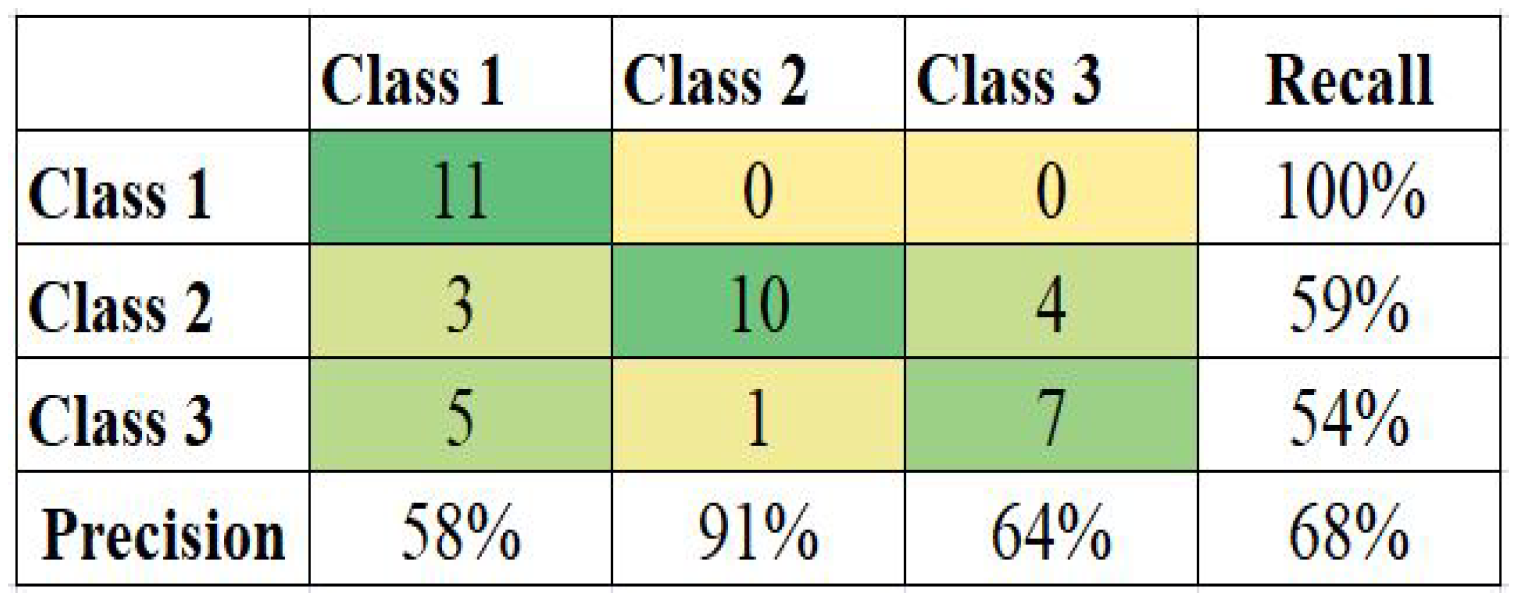
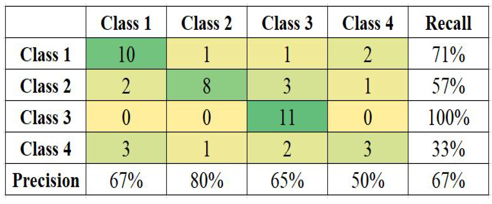
The model’s certainty to predict the class of the unknown samples correctly defines its efficiency, illustrated by various factors, like confusion matrix, accuracy, recall, and precision. The confusion matrix visualizes the performance of the model by producing numbers of samples predicted correctly and incorrectly. Precision, also known as Positive Predictive Value or PPV, is the fraction of cases when the model identifies the class of the sample correctly. Accuracy is the measure of correctly predicted sample points out of the complete data. Recall or sensitivity is the fraction of cases rightly identified as belonging to the respective class amidst all the samples that correctly fit that class. While evaluating the four datasets, all the four mentioned factors are considered. Figure 5, Figure 6, Figure 7 and Figure 8 present the confusion matrix and calculated Precision and Recall for each class for datasets of Ecuador, Haiti, Nepal, and South Korea. The (3 × 3) or (4 × 4) size of the confusion matrix follows the number of classes in the respective datasets.

Haiti model in Figure 6 shows the highest accuracy of 68%, and precision of 58%, 91%, and 64% for damage classes 1, 2, and 3, respectively. Class 1 building samples are efficiently classified, i.e., 11 out of 19, while Class 3 samples show a low acceptance, and only 7 out of 17 are predicted accurately.

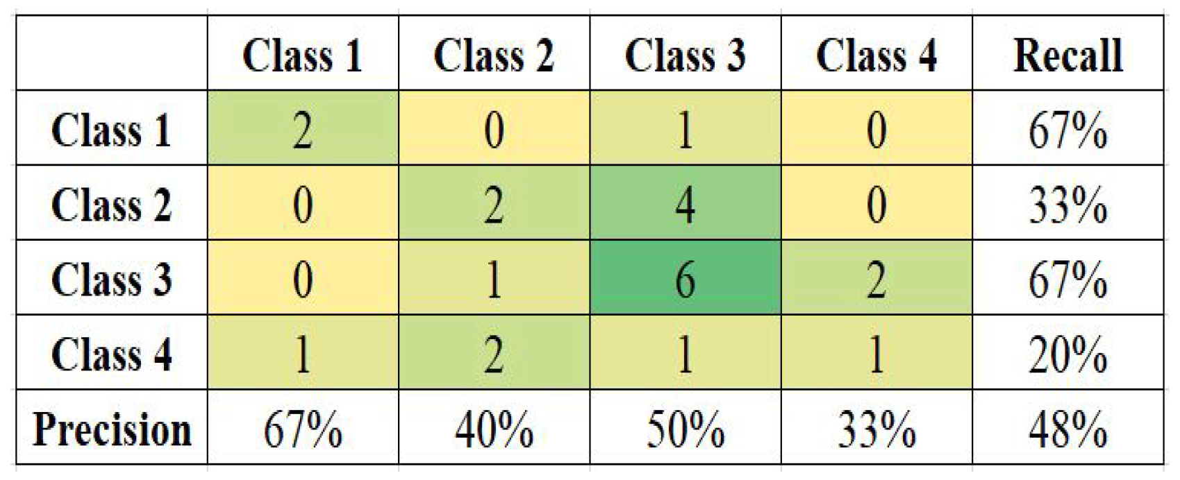
Among all the models, the South Korea model functioned with the least accuracy of 48%. A low number of sample data can be one of the reasons for the model’s lower accuracy. Class 1 and Class 3 have the highest and same recall value of 67%; it shows that these classes are correctly recognized, while class 4 is poorly misclassified with a recall value of only 20%.

To understand the practicality of balancing the imbalanced data, the study evaluated the model prediction efficiency before and after data manipulation.

Table 9. Model accuracy with and without imbalanced data.

Country	Imbalanced Data Accuracy and Kernel (%)	Balanced Data Accuracy and Kernel (%)
Ecuador	54 RBF	60 RBF
Haiti	52 RBF	68 RBF
Nepal	59 Sigmoid	67 RBF
South Korea	43 RBF	48 RBF

shows the accuracy of each model with the current kernel, achieved prior and later shaping of the imbalanced data. The accuracy of each model improved after balancing the imbalanced data. The highest accuracy of 68% for the Haiti model was only 60% when the data were imbalanced, whereas South Korea only had 43% accuracy, even lesser than 48%. Most results employed RBF kernels.

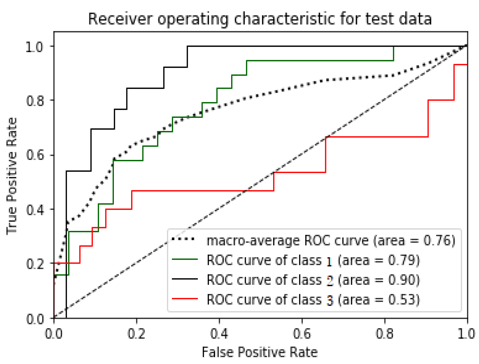
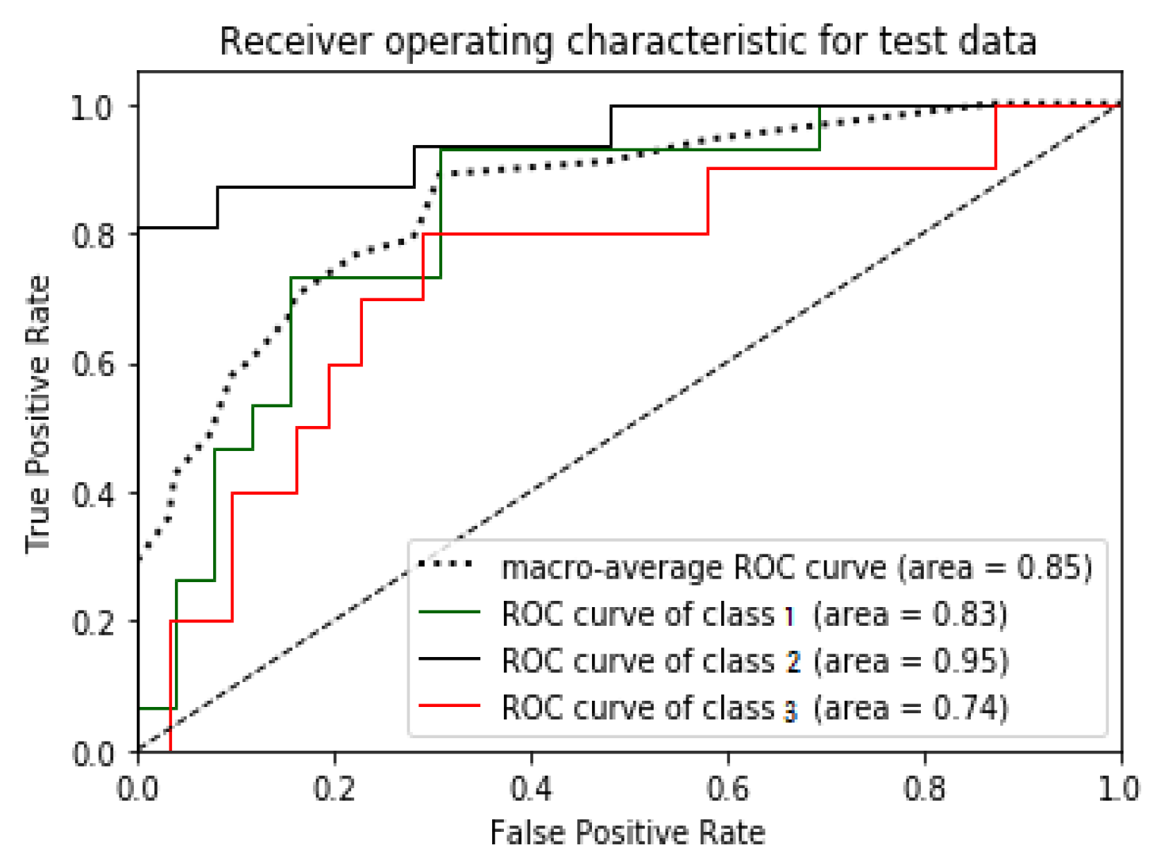
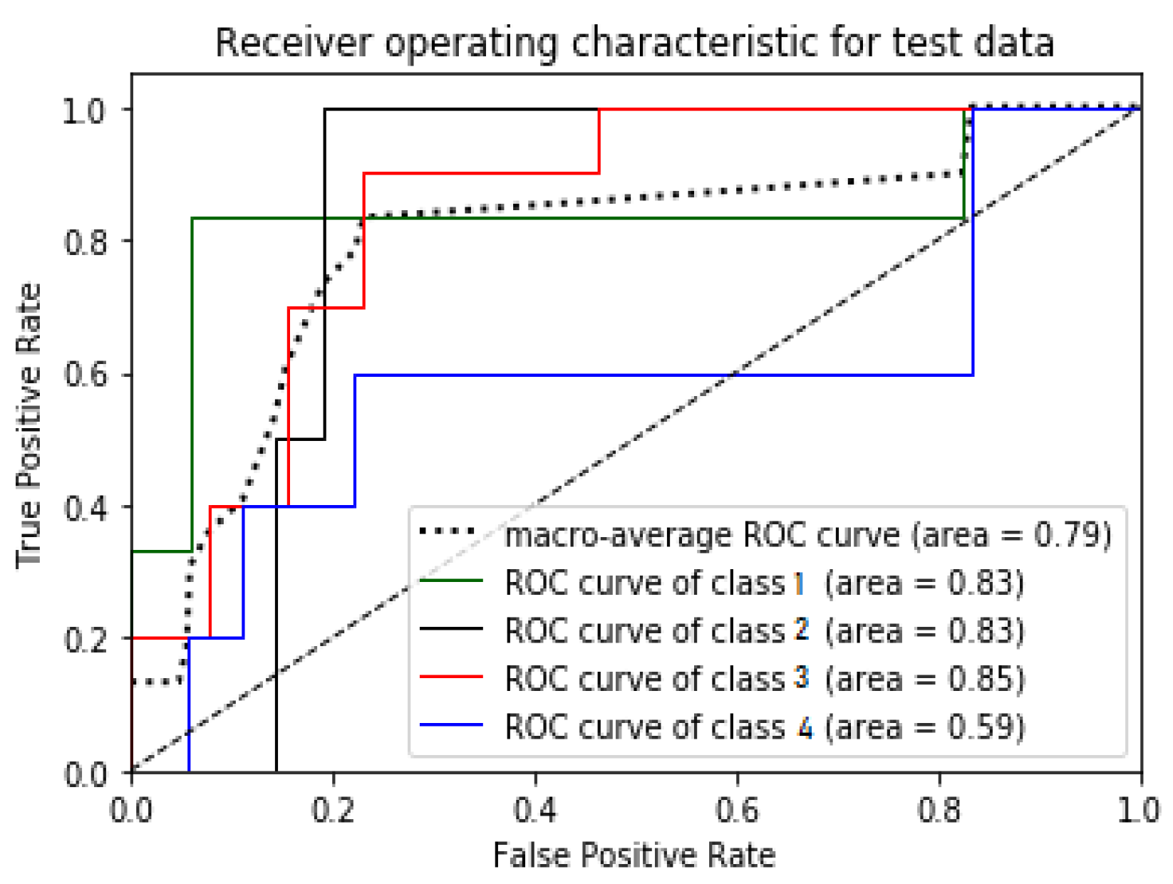
The Receiver Operating Characteristics (ROC) curve is represented by a graphical plot that depicts a binary classifier model’s indicative capacity as its bias threshold differs. The X-axis and Y-axis of the ROC curve display true positive and false positive, respectively. Therefore, the ROC plot’s top left corner acts as an “ideal” point—depicting value zero for a false positive rate and a true positive rate. Therefore, the larger the area under the curve (AUC), the better is the classifier performance. The ROC curve’s steepness serves an essential part in expanding the true positive rate and reducing the false-positive rate. Since the ROC curve works only in binary classification, a multi-class classification method needs to binarize the output. The curves of different classes generated in ROC are comparable with each other or with a varying threshold.

Figure 9, Figure 10, Figure 11 and Figure 12 illustrates the ROC plots for the test data for Ecuador, Haiti, Nepal, and South Korea models, respectively. Macro-average shown in the ROC curves is to evaluate multi-class classification problems. Macro-average computes the test data independently for each class and calculates the average.

ROC curves for Haiti (Figure 10) and Nepal (Figure 11) illustrate the better performance of their model over the test data with a probability of 85% and 84%, respectively. Figure 10 clearly shows that the model significantly classified test samples belonging to class 2 (95%), whereas test samples belonging to class 3 are moderately predicted (74%). As macro-averaging is the average of model performance for each class, Ecuador shows the least macro-average percentage (76%) with an efficiency of only 53% in classifying test samples belonging to the class 3. The proposed method results show a significant improvement in RVS methods such as RVS based on multi-criteria decision-making [19] or Multi-Layer Perceptron [13] where the accuracies were around 37% and 52%, respectively.

Additionally, the area under the curve (AUC) is also used for model performance evaluation as a summarized intelligence model. AUC is the probability of a model to put a positive sample in a higher rank than a negative chosen sample. Therefore, the more substantial area under the curve, the better the model.

Table 10. AUC score of classifiers.

Classifier	AUC Score (Macro)
Ecuador	0.740
Haiti	0.840
Nepal	0.826
South Korea	0.775

presents the AUC score achieved by each model.

6. Conclusions

Modern building designs respect the required safety norms while constructing multi-story and intricate architecture, and therefore they possess less risk when subjected to seismic vulnerability. However, existing residential and commercial buildings show several signs of low construction quality, lousy maintenance, and damage signs, further increasing if associated with an earthquake.

This study focused on the modern technique of RVS methods to analyze and minimize the risk factors associated with old and existing buildings. Machine learning is quick and cost-effective when the excellent quality of data is available. RC buildings sample data from four different countries Ecuador, Haiti, Nepal, and South Korea, are interpreted and evaluated using Machine Learning to scrutinize the damage scale for unseen samples. Eight input features, the number of stories, total floor area, column area, concrete wall area (X and Y), masonry wall area (X and Y), and captive columns are considered. The performance of the classifier is evaluated with imbalanced and balanced input data. Balanced data equally distribute the number of feature points among all the classes, by duplicating the data points from minor class, without making any significant change in the information. The classifier showed improved accuracy for each dataset with balanced data. Ecuador, Haiti, and Nepal datasets incurred an accuracy of 60%, 68%, and 67%, respectively, which illustrate that the classifier performed well over the unseen samples. The probable reason behind South Korea’s limited performance (less than 50%) could be fewer sample data. A classifier does not significantly evaluate new data if less training data are available, which weakens its learning capacity.

The future study can further extend to evaluate the SVM classifier’s performance with more data while examining each feature’s influence. The soft margin technique can also be implemented, replacing hyper-parameter tuning to study similar datasets for multi-class classification. Possibly k-fold cross-validation technique can also be used instead of GridSearch.