A Novel Explicit Analytical Multibody Approach for the Analysis of Upper Limb Dynamics and Joint Reactions Calculation Considering Muscle Wrapping

Featured Application

Explicit biomechanical multibody model for the inverse dynamics of upper limb musculoskeletal systems considering muscle wrapping.

Abstract

The aim of this paper is to present an explicit analytical biomechanical multibody procedure able to be implemented in the solution of the musculoskeletal systems inverse dynamics problems. The model is proposed in formal multibody analysis and implemented in the Matlab numerical environment. It is based on the constraint kinematical behaviour analysis and considers both linear muscle actuators and curved ones, by calculating the geodesic muscle path over wrapping surfaces fixed to the bodies. The model includes the Hill muscle approach in order to evaluate both the contractile elements’ actions and the passive ones. With the aim to have a first validation, the model was applied to the dynamical analysis of the “arm26” OpenSim model, an upper limb subjected to external forces of gravity and to known kinematics. The comparison of results shows interesting matching in terms of kinematical analysis, driving forces, muscles’ activations and joint reactions, proving the reliability of the proposed approach in all cases in which it is necessary to achieve in-silico explicit determinations of the upper limb dynamics and joint reactions (i.e., in joint tribological optimization).

1. Introduction

In the framework of biomechanics, the dynamics of the human body plays an important role: it is necessary to apply knowledge of the joint contact forces during certain human kinematics motion to analyse the joint loading, and to define the synovial joints (hip, knee, ankle, etc.) tribological behaviour and mechanical performances. It is necessary to estimate the friction and the wear of the articulated surfaces [1,2,3], to predict some articular diseases such as the osteoarthritis [4,5] and to design prostheses able to replace the worn natural joint [6,7,8] or to investigate the influence of some properties on the prosthesis performance [9,10,11], etc.

The in vitro or in vivo approaches to study biomechanical phenomena, are characterised by a wide deviation of the measurement results. Since they are dependent on many parameters and vary from subject to subject [12,13,14], many experiments are required to define an average behaviour of a certain physical system. For these reasons, the in silico approach is becoming a very suitable way to overcome the described issues, and many software, able to solve numerically dynamical musculoskeletal systems, have been developed by researchers, such as OpenSim, AnyBody, etc.

Each software is built with algorithms used to approach mathematical problems; despite them being computationally optimized to solve problems, they are not fully controllable and they are not easy to use as a subroutine in more complex models.

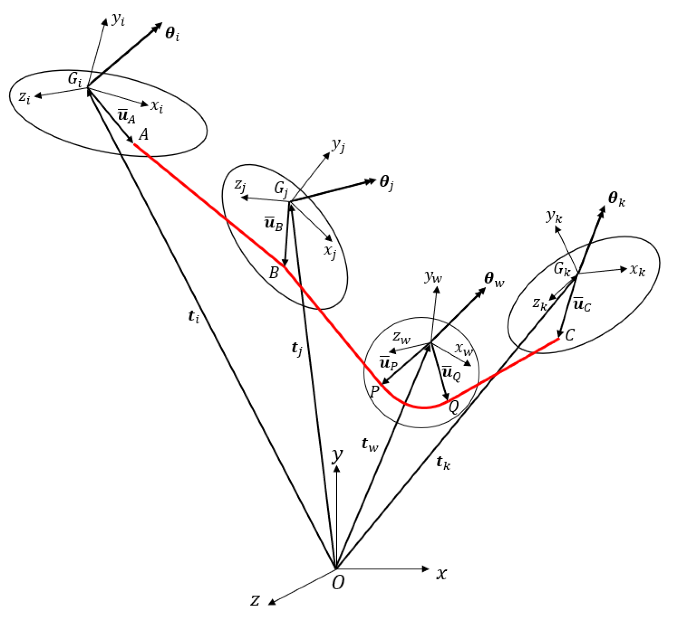
A musculoskeletal system can be seen as a set of bodies; the bones, linked by joints which, simultaneously, allow and constrain the relative motions between them. It is moved by a complex actuation system composed by “deformable actuators” attached to the bodies, the muscles, governed by neural excitation signals [15]. In order to analyse the joint contact forces of an articulated system subjected to a known motion, one of the best ways to achieve the goal is to solve the inverse dynamics problem with a multibody approach, after performing the scaling and the inverse kinematics [16] to adapt the musculoskeletal system to the particular subject and motion.

With reference to the above issues, an analysis of scientific literature furnishes interesting findings.

In [6] the authors analysed the differences between two multibody musculoskeletal models of the upper limb, an anatomical one and one provided with a reverse shoulder prosthesis. They focused on the comparison between the muscles’ lengths, forces and joint reactions by varying the shoulder replacement location and geometry.

In [9] the authors validated the quality of a multibody simulation in the framework of above-knee amputees subjects based on a socket. They compared the calculated loads acting on the socket interface with the ones acquired by measurement devices applied on six subjects during level walking captured in gait laboratories, obtaining good agreements.

In [11] the authors discussed the theoretical multibody approaches and contact simulations in the framework of mechanical hands so as to adapt them to prosthetic hands. They studied the dynamical behaviour of the finger and the phalanx in order to analyse the grasping ability of the artificial hand.

In [17] the authors proposed to associate a fatigue model to the muscle one, in a general multibody simulation, considering the muscular force history, to evaluate its fitness level. The authors, with reference to a simple upper extremity system subjected to gravity and a concentrated load, obtained interesting results in terms of the increase of the muscles activation and/or of the number of recruited muscles after a loss of force production capacity.

In [18] the authors furnished a detailed description of the main techniques used to solve the inverse dynamics of musculoskeletal systems, showing the joint modelling, the muscular tissue dynamics and the physiological criteria. They applied the model in the case of the gait analysis of a geometrically reliable whole body.

In [19] the authors showed the multibody analysis potential to solve problems in the framework of the craniofacial biomechanics of both human and non-human applications.

In [20] the authors performed an overview on the multibody kinematic optimization, focusing on the reliability of the kinematical analysis associated to the upper limb modelling with respect to the motion of the soft tissue artefacts, the skin, which in general provides errors.

In [21] the authors developed an interesting multibody model of the human spine by discretising the linked intervertebral discs by a series of rotational joints, obtaining reliable results and pointing out on the model utility in the framework of the seating systems comfort investigation and of the surgical field.

In the above scientific framework, the aim of this paper is to develop, step by step, an explicit analytical multibody model representing the “core model” of a novel algorithm written by the authors in the Matlab environment, able to solve the inverse dynamics of upper limb musculoskeletal systems, allowing the explicit control of the involved variables. The reliability of the model is evaluated by performing a comparison with the results of an inverse dynamics analysis obtained from the open-source software OpenSim on the upper limb system subjected to a known kinematics example.

2. Materials and Methods

2.1. Musculoskeletal System

From a general point of view, a multibody model firstly needs the topology of the system, namely the set of $n_B$ bodies and $n_J$ joints together with the information about which joint links the parent body to the child bodies. The parent body of a joint is the body in which the joint is defined in terms of reference frame, while the child bodies of a joint are the bodies subjected to the relative motion, linked through the joint to the parent body.

We assumed as reference model the OpenSim “arm26” [22] (Figure 1) together with the reference frames of the ground and the joints: it is composed of 3 bodies: the ground, the humerus and the forearm; these are denoted by the complex of the ulna-radius-hand and by 2 joints, the shoulder, which connects the humerus to the ground, and the elbow, which links the forearm to the humerus.

Each body $i$ in the space is described by Lagrangian coordinates ${\mathit{q}}_i$, (1), which is a vector of 7 elements composed of its mass centre $G_i$ translation with respect to the ground ${\mathit{t}}_i$ and its orientation with respect to the ground reference frame denoted by the unit quaternion ${\mathit{\theta }}_i$.

$$\begin{array}{c}{\mathit{q}}_i=\left[\begin{array}{c}{\mathit{t}}_i\\ {\mathit{\theta }}_i\end{array}\right]\end{array}$$

(1)

According to the quaternion theory [23], a unit quaternion $\mathit{\theta }$ is a unit vector composed of a scalar real part and a vector imaginary part, describing the orientation of a floating reference frame rotated with respect to a fixed one by the knowledge of the rotation angle and the axis around which it is performed. The information about the quaternion and its time derivatives allows calculating a body’s angular velocity $\mathit{\omega }$ together with the rotation matrix $\mathit{R}$ with respect to the ground reference frame. A kinematical analysis is necessary to elaborate the position ${\mathit{r}}_P$, the velocity ${\mathit{v}}_P$ or the acceleration ${\mathit{a}}_P$ of any point $P$ in the space (joint, muscle attachment point, external force application point, etc.) fixed to a body $i$, through its local position with respect to the body $i$, ${\overline{\mathit{u}}}_{P,i}$, the body’s Lagrangian coordinates ${\mathit{q}}_i$ and their derivatives ${\dot{\mathit{q}}}_i$ and ${\ddot{\mathit{q}}}_i$ [23], as described in (2).

$$\begin{array}{c}\begin{array}{c}{\mathit{r}}_P={\mathit{t}}_i+{\mathit{R}}_i{\overline{\mathit{u}}}_{P,i}\\ {\mathit{v}}_P={\dot{\mathit{t}}}_i-{\mathit{R}}_i{\widetilde{\overline{\mathit{u}}}}_{P,i}{\overline{\mathit{G}}}_i{\dot{\mathit{\theta }}}_i\\ {\mathit{a}}_P={\ddot{\mathit{t}}}_i-{\tilde{\mathit{\omega }}}_i{\mathit{R}}_i{\widetilde{\overline{\mathit{u}}}}_{P,i}{\overline{\mathit{G}}}_i{\dot{\mathit{\theta }}}_i-{\mathit{R}}_i{\widetilde{\overline{\mathit{u}}}}_{P,i}{\overline{\mathit{G}}}_i{\ddot{\mathit{\theta }}}_i\end{array}\end{array}$$

(2)

2.2. Kinematical Analysis Based on the Constraints

Since the time evolutions of the $n_{dof}$ system’s degrees of freedom are known, a kinematical analysis can be immediately performed. The analysis is based on the idea that the system has to satisfy during the time $t$ the set of constraint equations coming from the joints’ kinematical behaviour, through the right set of the bodies’ Lagrangian coordinates $\mathit{q}$ [24,25], obtained by concatenating the individual ones ${\mathit{q}}_i$ along the column direction.

A multibody system made of $n_B$ bodies (including the ground) which move in a known way, is subjected to the constraint equations composed by:

-

$n_{dof}$ rheonomic constraints which drive the degrees of freedom to move with the known trajectories (${\mathit{C}}_r$);

-

$n_c$ scleronomic constraints due to the relative motions blocked by the joints kinematical behaviour (${\mathit{C}}_s$);

-

$\left(n_B-1\right)$ constraints which guarantee that the bodies’ quaternions keep the unitary norm (${\mathit{C}}_b)$.

From the mobility Equation (3),

$$\begin{array}{c}{n}_{dof}=6\left(n_B-1\right)-n_c,\end{array}$$

(3)

the $7\left(n_B-1\right)$ constraint equations needed to find the same number of unknown $\mathit{q}$ are included in the constraint vector $\mathit{C}$ in (4).

$$\begin{array}{c}\mathit{C}\left(\mathit{q},t\right)=\left[\begin{array}{c}{\mathit{C}}_r\left(\mathit{q},t\right)\\ {\mathit{C}}_s\left(\mathit{q}\right)\\ {\mathit{C}}_b\left(\mathit{q}\right)\end{array}\right]=0\end{array}$$

(4)

The kinematical analysis, in (5), can be performed by solving the closed non-linear system of equations $\mathit{C}$ through the Newton iterative method for the position problem and by differentiating the constraints with respect to time $t$, obtaining two linear systems to solve the velocity and acceleration, which provide the Lagrangian velocities $\dot{\mathit{q}}$ and accelerations $\ddot{\mathit{q}}$.

$$\begin{array}{c}\begin{array}{c}{\mathit{q}}^{\left(k+1\right)}={\mathit{q}}^{\left(k\right)}-{\mathit{C}}_{\mathit{q}}^{-1}\left({\mathit{q}}^{\left(k\right)},t\right)\mathit{C}\left({\mathit{q}}^{\left(k\right)},t\right)\\ {\mathit{C}}_{\mathit{q}}\dot{q}=-{\mathit{C}}_t\\ {\mathit{C}}_{\mathit{q}}\ddot{\mathit{q}}=-\left({\dot{\mathit{C}}}_t+{\dot{\mathit{C}}}_{\mathit{q}}\dot{\mathit{q}}\right)\end{array}\end{array}$$

(5)

The constraint Jacobian ${\mathit{C}}_{\mathit{q}}$ and the other matrices and vectors involved in the kinematical analysis in (5) ($\mathit{C}$, ${\mathit{C}}_t$,${\dot{\mathit{C}}}_{\mathit{q}}$, ${\dot{\mathit{C}}}_t$), are obtained by analysing the joints kinematical behaviour. In this application the shoulder and the elbow are modelled as revolute joints, so only this joint type is discussed. A revolute joint $J$ allows only a relative rotation $\theta$ between the linked bodies $i$ and $j$ around an axis defined by the unit vector $\widehat{\mathit{v}}$ fixed to the parent body $i$, as showed in the Figure 2.

The rheonomic constraint $C_{r,J}$ associated to the revolute joint $J$ is generally modelled considering that the scalar product between two particular vectors fixed to the related bodies has to be equal to the cosine of the relative rotation $\theta$ [18,25]: the periodicity of the trigonometric functions does not allow to reaching a unique solution numerically solving the position analysis. In this work this particular constraint is modelled considering that the difference between the bodies’ absolute angular coordinates $\mathit{\phi }$ projected on the rotation axis $\widehat{\mathit{v}}$ has to be equal to the relative rotation $\theta$, as written in (6).

$$\begin{array}{c}{C}_{r,J}\left(\mathit{q},t\right)={\widehat{\mathit{v}}}^T{\mathit{R}}_i^T\left({\mathit{\phi }}_j-{\mathit{\phi }}_i\right)-\theta \left(t\right)=0\end{array}$$

(6)

The related scleronomic constraints ${\mathit{C}}_{s,J}$ are composed of a translational part and a rotational one [25], in (7):

-

the joint position calculated starting from the body $i$, ${\mathit{r}}_{J,i}$, has to be equal to the one seen by the body $j$, ${\mathit{r}}_{J,j}$;

-

a vector fixed to body $j$, ${\overline{\mathit{s}}}_j$, parallel to the rotation axis $\widehat{\mathit{v}}$, has to be orthogonal with respect to others two vectors fixed to the body $i$, ${\overline{\mathit{s}}}_{i1}$ and ${\overline{\mathit{s}}}_{i2}$, both orthogonal to the rotation axis $\widehat{\mathit{v}}$ and to each other.

$$\begin{array}{c}\{\begin{array}{c}{\mathit{r}}_{J,i}={\mathit{t}}_i+{\mathit{R}}_i{\overline{\mathit{u}}}_{J,i}\\ {\mathit{r}}_{J,j}={\mathit{t}}_j+{\mathit{R}}_j{\overline{\mathit{u}}}_{J,j}\\ {\mathit{s}}_j={\mathit{R}}_j{\overline{\mathit{s}}}_j\\ {\mathit{s}}_{i1}={\mathit{R}}_i{\overline{\mathit{s}}}_{i1}\\ {\mathit{s}}_{i2}={\mathit{R}}_i{\overline{\mathit{s}}}_{i2}\end{array} \to {\mathit{C}}_{s,J}\left(\mathit{q}\right)=\left[\begin{array}{c}{\mathit{r}}_{J,i}-{\mathit{r}}_{J,j}\\ {\mathit{s}}_{i1}^T{\mathit{s}}_j\\ {\mathit{s}}_{i2}^T{\mathit{s}}_j\end{array}\right]=\mathbf{0}\end{array}$$

(7)

While the joint local positions ${\overline{\mathit{u}}}_{J,i}$ and ${\overline{\mathit{u}}}_{J,j}$ are provided by the geometry of the system, the vectors ${\overline{\mathit{s}}}_j$, ${\overline{\mathit{s}}}_{i1}$ and ${\overline{\mathit{s}}}_{i2}$ can be calculated considering the spherical transformation that rotates the reference frame of the body $i$ or $j$ leading the $x$ axis to be parallel with respect to the rotation axis $\widehat{\mathit{v}}$.

The time derivatives of the rheonomic constraint are then performed in (8) (considering that from the quaternion theory results $\dot{\mathit{G}}\dot{\mathit{\theta }}=\mathbf{0}$).

$$\begin{array}{c}{\dot{C}}_{r,J}\left(\mathit{q},\dot{\mathit{q}},t\right)=-{\widehat{\mathit{v}}}^T{\overline{\mathit{G}}}_i{\dot{\mathit{\theta }}}_i+{\widehat{\mathit{v}}}^T{\mathit{R}}_i^T{\mathit{R}}_j{\overline{\mathit{G}}}_j{\dot{\mathit{\theta }}}_j-\dot{\theta }\left(t\right)=0\\ {\ddot{C}}_{r,J}\left(\mathit{q},\dot{\mathit{q}},\ddot{\mathit{q}},t\right)=-{\widehat{\mathit{v}}}^T{\overline{\mathit{G}}}_i{\ddot{\mathit{\theta }}}_i+{\widehat{\mathit{v}}}^T{\mathit{R}}_i^T{\mathit{R}}_j{\overline{\mathit{G}}}_j{\ddot{\mathit{\theta }}}_j+{\widehat{\mathit{v}}}^T{\mathit{R}}_i^T{\tilde{\mathit{\omega }}}_i^T{\mathit{R}}_j{\overline{\mathit{G}}}_j{\dot{\mathit{\theta }}}_j+{\widehat{\mathit{v}}}^T{\mathit{R}}_i^T{\tilde{\mathit{\omega }}}_j{\mathit{R}}_j{\overline{\mathit{G}}}_j{\dot{\mathit{\theta }}}_j-\ddot{\theta }\left(t\right)=0\end{array}$$

(8)

Collecting the terms in order to build the matrices needed for the kinematical analysis, Equation (9) is obtained.

$$\begin{array}{c}{\dot{C}}_{r,J}=\left[\begin{array}{cc}\mathbf{0}& -{\widehat{\mathit{v}}}^T{\overline{\mathit{G}}}_i\end{array}\right]\left[\begin{array}{c}{\dot{\mathit{t}}}_i\\ {\dot{\mathit{\theta }}}_i\end{array}\right]+\left[\begin{array}{cc}\mathbf{0}& {\widehat{\mathit{v}}}^T{\mathit{R}}_i^T{\mathit{R}}_j{\overline{\mathit{G}}}_j\end{array}\right]\left[\begin{array}{c}{\dot{\mathit{t}}}_j\\ {\dot{\mathit{\theta }}}_j\end{array}\right]-\dot{\theta }\left(t\right)=0\\ {\ddot{C}}_{r,J}=\left[\begin{array}{cc}\mathbf{0}& -{\widehat{\mathit{v}}}^T{\overline{\mathit{G}}}_i\end{array}\right]\left[\begin{array}{c}{\ddot{\mathit{t}}}_i\\ {\ddot{\mathit{\theta }}}_i\end{array}\right]+\left[\begin{array}{cc}\mathbf{0}& {\widehat{\mathit{v}}}^T{\mathit{R}}_i^T{\mathit{R}}_j{\overline{\mathit{G}}}_j\end{array}\right]\left[\begin{array}{c}{\ddot{\mathit{t}}}_j\\ {\ddot{\mathit{\theta }}}_j\end{array}\right]+\mathbf{0}\left[\begin{array}{c}{\dot{\mathit{t}}}_i\\ {\dot{\mathit{\theta }}}_i\end{array}\right]+\left[\begin{array}{cc}\mathbf{0}& {\widehat{\mathit{v}}}^T{\mathit{R}}_i^T\left({\tilde{\mathit{\omega }}}_i^T+{\tilde{\mathit{\omega }}}_j\right){\mathit{R}}_j{\overline{\mathit{G}}}_j\end{array}\right][\begin{array}{c}{\dot{\mathit{t}}}_j\\ {\dot{\mathit{\theta }}}_j\end{array}]-\ddot{\theta }\left(t\right)=0\end{array}$$

(9)

The same logic is adopted in order to find the time derivatives of the scleronomic constraints in (10).

$$\begin{array}{c}{\dot{\mathit{C}}}_{s,J}\left(\mathit{q},\dot{\mathit{q}}\right)=\left[\begin{array}{l}{\dot{\mathit{t}}}_i-{\mathit{R}}_i{\widetilde{\overline{\mathit{u}}}}_{J,i}{\overline{\mathit{G}}}_i{\dot{\mathit{\theta }}}_i-{\dot{\mathit{t}}}_j+{\mathit{R}}_j{\widetilde{\overline{\mathit{u}}}}_{J,j}{\overline{\mathit{G}}}_j{\dot{\mathit{\theta }}}_j\\ -{\overline{\mathit{s}}}_j^T{\mathit{R}}_j^T{\mathit{R}}_i{\widetilde{\overline{\mathit{s}}}}_{i1}{\overline{\mathit{G}}}_i{\dot{\mathit{\theta }}}_i-{\overline{\mathit{s}}}_{i1}^T{\mathit{R}}_i^T{\mathit{R}}_j{\widetilde{\overline{\mathit{s}}}}_j{\overline{\mathit{G}}}_j{\dot{\mathit{\theta }}}_j\\ -{\overline{\mathit{s}}}_j^T{\mathit{R}}_j^T{\mathit{R}}_i{\widetilde{\overline{\mathit{s}}}}_{i2}{\overline{\mathit{G}}}_i{\dot{\mathit{\theta }}}_i-{\overline{\mathit{s}}}_{i2}^T{\mathit{R}}_i^T{\mathit{R}}_j{\widetilde{\overline{\mathit{s}}}}_j{\overline{\mathit{G}}}_j{\dot{\mathit{\theta }}}_j\end{array}\right]=\mathbf{0}\\ {\ddot{\mathit{C}}}_{s,J}\left(\mathit{q},\dot{\mathit{q}},\ddot{\mathit{q}}\right)=\left[\begin{array}{c}{\ddot{\mathit{t}}}_i\mathit{-}{R}_i{\widetilde{\overline{\mathit{u}}}}_{J,i}{\overline{\mathit{G}}}_i{\ddot{\mathit{\theta }}}_i-{\mathit{R}}_i{\widetilde{\overline{\mathit{\omega }}}}_i{\widetilde{\overline{\mathit{u}}}}_{J,i}{\overline{\mathit{G}}}_i{\dot{\mathit{\theta }}}_i-{\ddot{\mathit{t}}}_j+{\mathit{R}}_j{\widetilde{\overline{\mathit{u}}}}_{J,j}{\overline{\mathit{G}}}_j{\ddot{\mathit{\theta }}}_j+{\mathit{R}}_j{\widetilde{\overline{\mathit{\omega }}}}_j{\widetilde{\overline{\mathit{u}}}}_{J,j}{\overline{\mathit{G}}}_j{\dot{\mathit{\theta }}}_j\\ -{\overline{\mathit{s}}}_j^T{\mathit{R}}_j^T{\mathit{R}}_i{\widetilde{\overline{\mathit{s}}}}_{i1}{\overline{\mathit{G}}}_i{\ddot{\mathit{\theta }}}_i-{\overline{\mathit{s}}}_j^T{\mathit{R}}_j^T\left({\tilde{\mathit{\omega }}}_j^T+{\tilde{\mathit{\omega }}}_i\right){\mathit{R}}_i{\widetilde{\overline{\mathit{s}}}}_{i1}{\overline{\mathit{G}}}_i{\dot{\mathit{\theta }}}_i-{\overline{\mathit{s}}}_{i1}^T{\mathit{R}}_i^T{\mathit{R}}_j{\widetilde{\overline{\mathit{s}}}}_j{\overline{\mathit{G}}}_j{\ddot{\mathit{\theta }}}_j-{\overline{\mathit{s}}}_{i1}^T{\mathit{R}}_i^T\left({\tilde{\mathit{\omega }}}_i^T+{\tilde{\mathit{\omega }}}_j\right){\mathit{R}}_j{\widetilde{\overline{\mathit{s}}}}_j{\overline{\mathit{G}}}_j{\dot{\mathit{\theta }}}_j\\ -{\overline{\mathit{s}}}_j^T{\mathit{R}}_j^T{\mathit{R}}_i{\widetilde{\overline{\mathit{s}}}}_{i2}{\overline{\mathit{G}}}_i{\ddot{\mathit{\theta }}}_i-{\overline{\mathit{s}}}_j^T{\mathit{R}}_j^T\left({\tilde{\mathit{\omega }}}_j^T+{\tilde{\mathit{\omega }}}_i\right){\mathit{R}}_i{\widetilde{\overline{\mathit{s}}}}_{i2}{\overline{\mathit{G}}}_i{\dot{\mathit{\theta }}}_i-{\overline{\mathit{s}}}_{i2}^T{\mathit{R}}_i^T{\mathit{R}}_j{\widetilde{\overline{\mathit{s}}}}_j{\overline{\mathit{G}}}_j{\ddot{\mathit{\theta }}}_j-{\overline{\mathit{s}}}_{i2}^T{\mathit{R}}_i^T\left({\tilde{\mathit{\omega }}}_i^T+{\tilde{\mathit{\omega }}}_j\right){\mathit{R}}_j{\widetilde{\overline{\mathit{s}}}}_j{\overline{\mathit{G}}}_j{\dot{\mathit{\theta }}}_j\end{array}\right]=\mathbf{0}\end{array}$$

(10)

Collecting the terms again, Equation (11) is obtained.

$$\begin{array}{c}{\dot{\mathit{C}}}_{s,J}=\left[\begin{array}{cc}\mathit{I}& -{\mathit{R}}_i{\widetilde{\overline{\mathit{u}}}}_{J,i}{\overline{\mathit{G}}}_i\\ \mathbf{0}& -{\overline{\mathit{s}}}_j^T{\mathit{R}}_j^T{\mathit{R}}_i{\widetilde{\overline{\mathit{s}}}}_{i1}{\overline{\mathit{G}}}_i\\ \mathbf{0}& -{\overline{\mathit{s}}}_j^T{\mathit{R}}_j^T{\mathit{R}}_i{\widetilde{\overline{\mathit{s}}}}_{i2}{\overline{\mathit{G}}}_i\end{array}\right]\left[\begin{array}{c}{\dot{\mathit{t}}}_i\\ {\dot{\mathit{\theta }}}_i\end{array}\right]+\left[\begin{array}{cc}-\mathit{I}& {\mathit{R}}_j{\widetilde{\overline{\mathit{u}}}}_{J,j}{\overline{\mathit{G}}}_j\\ \mathbf{0}& -{\overline{\mathit{s}}}_{i1}^T{\mathit{R}}_i^T{\mathit{R}}_j{\widetilde{\overline{\mathit{s}}}}_j{\overline{\mathit{G}}}_j\\ \mathbf{0}& -{\overline{\mathit{s}}}_{i2}^T{\mathit{R}}_i^T{\mathit{R}}_j{\widetilde{\overline{\mathit{s}}}}_j{\overline{\mathit{G}}}_j\end{array}\right]\left[\begin{array}{c}{\dot{\mathit{t}}}_j\\ {\dot{\mathit{\theta }}}_j\end{array}\right]=\mathbf{0}\\ {\ddot{\mathit{C}}}_{s,J}=\left[\begin{array}{cc}\mathit{I}& -{\mathit{R}}_i{\widetilde{\overline{\mathit{u}}}}_{J,i}{\overline{\mathit{G}}}_i\\ \mathbf{0}& -{\overline{\mathit{s}}}_j^T{\mathit{R}}_j^T{\mathit{R}}_i{\widetilde{\overline{\mathit{s}}}}_{i1}{\overline{\mathit{G}}}_i\\ \mathbf{0}& -{\overline{\mathit{s}}}_j^T{\mathit{R}}_j^T{\mathit{R}}_i{\widetilde{\overline{\mathit{s}}}}_{i2}{\overline{\mathit{G}}}_i\end{array}\right]\left[\begin{array}{c}{\ddot{\mathit{t}}}_i\\ {\ddot{\mathit{\theta }}}_i\end{array}\right]+\left[\begin{array}{cc}-\mathit{I}& {\mathit{R}}_j{\widetilde{\overline{\mathit{u}}}}_{J,j}{\overline{\mathit{G}}}_j\\ \mathbf{0}& -{\overline{\mathit{s}}}_{i1}^T{\mathit{R}}_i^T{\mathit{R}}_j{\widetilde{\overline{\mathit{s}}}}_j{\overline{\mathit{G}}}_j\\ \mathbf{0}& -{\overline{\mathit{s}}}_{i2}^T{\mathit{R}}_i^T{\mathit{R}}_j{\widetilde{\overline{\mathit{s}}}}_j{\overline{\mathit{G}}}_j\end{array}\right]\left[\begin{array}{c}{\ddot{\mathit{t}}}_j\\ {\ddot{\mathit{\theta }}}_j\end{array}\right]+\left[\begin{array}{cc}\mathbf{0}& -{\mathit{R}}_i{\widetilde{\overline{\mathit{\omega }}}}_i{\widetilde{\overline{\mathit{u}}}}_{J,i}{\overline{\mathit{G}}}_i\\ \mathbf{0}& -{\overline{\mathit{s}}}_j^T{\mathit{R}}_j^T\left({\tilde{\mathit{\omega }}}_j^T+{\tilde{\mathit{\omega }}}_i\right){\mathit{R}}_i{\widetilde{\overline{\mathbf{s}}}}_{i1}{\overline{\mathit{G}}}_i\\ \mathbf{0}& -{\overline{\mathit{s}}}_j^T{\mathit{R}}_j^T\left({\tilde{\mathit{\omega }}}_j^T+{\tilde{\mathit{\omega }}}_i\right){\mathit{R}}_i{\widetilde{\overline{\mathit{s}}}}_{i2}{\overline{\mathit{G}}}_i\end{array}\right]\left[\begin{array}{c}{\dot{\mathit{t}}}_i\\ {\dot{\mathit{\theta }}}_i\end{array}\right]+\left[\begin{array}{cc}\mathbf{0}& {\mathit{R}}_j{\widetilde{\overline{\mathit{\omega }}}}_j{\widetilde{\overline{\mathit{u}}}}_{J,j}{\overline{\mathit{G}}}_j\\ \mathbf{0}& -{\overline{\mathit{s}}}_{i1}^T{\mathit{R}}_i^T\left({\tilde{\mathit{\omega }}}_i^T+{\tilde{\mathit{\omega }}}_j\right){\mathit{R}}_j{\widetilde{\overline{\mathit{s}}}}_j{\overline{\mathit{G}}}_j\\ \mathbf{0}& -{\overline{\mathit{s}}}_{i2}^T{\mathit{R}}_i^T\left({\tilde{\mathit{\omega }}}_i^T+{\tilde{\mathit{\omega }}}_j\right){\mathit{R}}_j{\widetilde{\overline{\mathit{s}}}}_j{\overline{\mathit{G}}}_j\end{array}\right]\left[\begin{array}{c}{\dot{\mathit{t}}}_j\\ {\dot{\mathit{\theta }}}_j\end{array}\right]=\mathbf{0}\end{array}$$

(11)

Once the rheonomic and scleronomic constraints are evaluated, the ones related to the quaternions’ unitary norm are written for each body $i$ in (12).

$$\begin{array}{c}{C}_{b.i}\left(\mathit{q}\right)={\mathit{\theta }}_i^T{\mathit{\theta }}_i-1=0\end{array}$$

(12)

The time derivatives of $C_{b,i}$ are evaluated in (13).

$$\begin{array}{c}\begin{array}{c}{\dot{C}}_{b,i}\left(\mathit{q},\dot{\mathit{q}}\right)=2{\mathit{\theta }}_i^T{\dot{\mathit{\theta }}}_i=0\\ {\ddot{C}}_{b,i}\left(\mathit{q},\dot{\mathit{q}},\ddot{\mathit{q}}\right)=2{\mathit{\theta }}_i^T{\ddot{\mathit{\theta }}}_i+2{\dot{\mathit{\theta }}}_i^T{\dot{\mathit{\theta }}}_i=0\end{array}\end{array}$$

(13)

Collecting the terms for the last time, Equation (14) is written.

$$\begin{array}{c}\begin{array}{c}{\dot{C}}_{b,i}=\left[\begin{array}{cc}\mathbf{0}& 2{\mathit{\theta }}_i^T\end{array}\right]\left[\begin{array}{c}{\dot{\mathit{t}}}_i\\ {\dot{\mathit{\theta }}}_i\end{array}\right]=0\\ {\ddot{C}}_{b,i}=\left[\begin{array}{cc}\mathbf{0}& 2{\mathit{\theta }}_i^T\end{array}\right]\left[\begin{array}{c}{\ddot{\mathit{t}}}_i\\ {\ddot{\mathit{\theta }}}_i\end{array}\right]+\left[\begin{array}{cc}\mathbf{0}& 2{\dot{\mathit{\theta }}}_i^T\end{array}\right]\left[\begin{array}{c}{\dot{\mathit{t}}}_i\\ {\dot{\mathit{\theta }}}_i\end{array}\right]=0\end{array}\end{array}$$

(14)

Every constraint $k$ is written in the form of (15) in order to extrapolate the needed submatrices that have to be associated to the related $i$ and $j$ bodies’ Lagrangian coordinates, so that the kinematical analysis can be solved. With reference to Equation (6), it is worth noting that the rheonomic constraint equations ${\mathit{C}}_r$ are written in such a way as to separate the functional dependence on the Lagrangian coordinates $\mathit{q}$, through the vector $\mathit{a}$, and the one on the time $t$, through the set of degrees of freedom ${\mathit{q}}_{dof}$.

$$\{\begin{array}{c}{\mathit{C}}_r\left(\mathit{q},t\right)=\mathit{a}\left(\mathit{q}\right)-{\mathit{q}}_{dof}\left(t\right)\\ {\mathit{C}}_{r,t}=-{\dot{\mathit{q}}}_{dof}\\ {\mathit{C}}_{r,tt}=-{\ddot{\mathit{q}}}_{dof}\end{array}\to \{\begin{array}{c}{\mathit{C}}_k\left(\mathit{q},t\right)=\mathbf{0}\\ {\dot{\mathit{C}}}_k\left(\mathit{q},\dot{\mathit{q}},t\right)={\mathit{C}}_{\mathit{q},i}{\dot{\mathit{q}}}_i+{\mathit{C}}_{\mathit{q},j}{\dot{\mathit{q}}}_j+{\mathit{C}}_{t,k}=\mathbf{0}\\ {\ddot{\mathit{C}}}_k\left(\mathit{q},\dot{\mathit{q}},\ddot{\mathit{q}},t\right)={\mathit{C}}_{\mathit{q},i}{\ddot{\mathit{q}}}_i+{\mathit{C}}_{\mathit{q},j}{\ddot{\mathit{q}}}_j+{\dot{\mathit{C}}}_{\mathit{q},i}{\dot{\mathit{q}}}_i+{\dot{\mathit{C}}}_{\mathit{q},j}{\dot{\mathit{q}}}_j+{\dot{\mathit{C}}}_{t,k}=\mathbf{0}\end{array}$$

(15)

2.3. Inverse Dynamics

The solution over time of the kinematical problem provides all the quantities needed for the inverse dynamics. In particular, with reference to the chosen generalised coordinates ${\mathit{q}}_i$, the equation of motion includes the mass matrix $\mathit{M}$, the vector of the centrifugal and Coriolis generalised force ${\mathit{Q}}_v$ and the external generalised force ${\mathit{Q}}_e$ [23] and it is written in the form of virtual work for a virtual displacement $\delta \mathit{q}$ by including the work of the internal forces through the constraint Jacobian ${\mathit{C}}_{\mathit{q}}$ and the Lagrange multipliers $\mathit{\lambda }$ in (16).

$$\begin{array}{c}\delta {\mathit{q}}^T\left(\mathit{M}\ddot{\mathit{q}}-{\mathit{Q}}_v-{\mathit{Q}}_e+{\mathit{C}}_{\mathit{q}}^T\mathit{\lambda }\right)=0 \end{array}$$

(16)

Since the work of the internal forces is considered, the equation of motion (22) is satisfied for any virtual displacement $\delta \mathit{q}$: in order to refer the bodies’ orientations to the local cartesian angular coordinates ${\overline{\mathit{\phi }}}_i$, instead of the quaternion ${\mathit{\theta }}_i$, a coordinate change is performed through the matrix ${\mathit{J}}_{\mathit{q}}$ [23], in (17).

$$\begin{array}{c}\delta {\mathit{q}}_i=\left[\begin{array}{c}\delta {\mathit{t}}_i\\ \delta {\mathit{\theta }}_i\end{array}\right]=\left[\begin{array}{cc}\mathit{I}& \mathbf{0}\\ \mathbf{0}& \frac{1}{4}{\overline{\mathit{G}}}_i^T\end{array}\right]\left[\begin{array}{c}\delta {\mathit{t}}_i\\ \delta {\overline{\mathit{\phi }}}_i\end{array}\right]={\mathit{J}}_{\mathit{q},i}\delta {\overline{\mathit{q}}}_i \to \delta {\overline{\mathit{q}}}^T{\mathit{J}}_{\mathit{q}}^T\left(\mathit{M}\ddot{\mathit{q}}-{\mathit{Q}}_v-{\mathit{Q}}_e+{\mathit{C}}_{\mathit{q}}^T\mathit{\lambda }\right)=0\end{array}$$

(17)

The generalised force vector ${\mathit{Q}}_c$ and the new constraint Jacobian ${\mathit{C}}_{\overline{\mathit{q}}}$ are defined in (18), leading to the final form of the multibody equation of motion.

$$\begin{array}{c}\{\begin{array}{c}{\mathit{Q}}_c={\mathit{J}}_{\mathit{q}}^T\left(\mathit{M}\ddot{\mathit{q}}-{\mathit{Q}}_v-{\mathit{Q}}_e\right)\\ {\mathit{C}}_{\overline{\mathit{q}}}={\mathit{C}}_{\mathit{q}}{\mathit{J}}_{\mathit{q}}\end{array} \to {\mathit{C}}_{\overline{\mathit{q}}}^T\mathit{\lambda }+{\mathit{Q}}_c=\mathbf{0}\end{array}$$

(18)

The coordinate transformation in (17) allows neglecting the part of the Jacobian associated with the constraints needed to keep the quaternions’ unitary norm: then Equation (18) becomes a closed linear system in which the unknowns are the Lagrange multipliers associated with the rheonomic constraints ${\mathit{\lambda }}_r$, representing the driving forces associated to each degree of freedom, and the ones related to the scleronomic constraints ${\mathit{\lambda }}_s$ [25], as showed in (19).

$$\begin{array}{c}\{\begin{array}{c}{\mathit{C}}_{\overline{\mathit{q}}}=\left[\begin{array}{c}{\mathit{C}}_{\overline{\mathit{q}},r}\\ {\mathit{C}}_{\overline{\mathit{q}},s}\end{array}\right]\\ \mathit{\lambda }=\left[\begin{array}{c}{\mathit{\lambda }}_r\\ {\mathit{\lambda }}_s\end{array}\right]\end{array} \to \left[\begin{array}{cc}{\mathit{C}}_{\overline{\mathit{q}},r}^T& {\mathit{C}}_{\overline{\mathit{q}},s}^T\end{array}\right]\left[\begin{array}{c}{\mathit{\lambda }}_r\\ {\mathit{\lambda }}_s\end{array}\right]=-{\mathit{Q}}_c\end{array}$$

(19)

The scleronomic multipliers ${\mathit{\lambda }}_s$ are not equal to the joint reaction forces, because the actuation of the musculoskeletal system doesn’t associate a single actuator to each degree of freedom: there are more muscles than degrees of freedom (redundancy) and, moreover, the muscular action is composed of a passive part which has to be considered as a known external force. In order to evaluate muscle forces and joint reactions, a muscle model is needed.

2.4. Hill Muscle Model

The Hill muscle model considers the muscle–tendon unit as a linear actuator between two attachment points $A$ and $B$ on the linked bodies (Figure 3) composed by the series of the tendon SE with length $l_t$ and the muscle, that is modelled as a parallel between the contractile element CE and the passive element PE, with length $l_m$ and inclined with respect to the action line by the pennation angle ${\alpha }_p$ [26,27,28].

The force $F_m$ generated by the muscle–tendon series is shared by the tendon and the muscle, so it can be evaluated as the sum of the ones generated by the contractile element $F_{CE}$, representing the active action due to the sarcomeres’ contractions, and the passive element $F_{PE}$, due to the muscular fibre tissue stiffness, projected on the action line through the pennation angle ${\alpha }_p$. The active part $F_{CE}$ depends on the activation level $a$, a scalar number between 0 and 1 determined by the muscular recruitment criterion, the muscle fibre length $l_m$ and deformation velocity $v_m$ through the force–length–velocity relationships, while the passive force $F_{PE}$ depends only on the muscle fibre length $l_m$ [28,29,30], as written in (20) and depicted in the Figure 4:

-

according to the force–length relation $f_l$, increasing the muscle fibre length, the active force increases until it reaches a peak (the maximum isometric force $F_0$) in correspondence with the optimal fibre length $l_0$, then it decreases;

-

the muscle generates a greater force than the maximum isometric one (in correspondence of zero deformation velocity) when it lengthens, with an asymptotic behaviour, and a lower force until it reaches the maximum contraction velocity $v_{max}$, beyond which it is not able to produce actuation, following the force–velocity relation $f_v$;

-

the passive element opposes a growing resistance only if the muscle length is greater than the optimal fibre length $l_0$, until it reaches a maximum value following the relation $f_{PE}$.

$$\begin{array}{c}\{\begin{array}{c}\tilde{l}=\frac{l_m}{l_0}\\ \tilde{v}=\frac{v_m}{v_{max}}\end{array} \to \{\begin{array}{c}{F}_{CE}=a{f}_l\left(\tilde{l}\right)f_v\left(\tilde{v}\right)F_0\\ F_{PE}=f_{PE}\left(\tilde{l}\right)F_0\end{array} \to F_m=\left(F_{CE}+F_{PE}\right)\cos {\alpha }_p\end{array}$$

(20)

Generally it is assumed that the tendon dynamics is negligible, so that the tendon length $l_t$ can be considered as a constant, and that the muscle width $w_m$ keeps constant values, even in correspondence of the muscle optimal fibre length $l_0$, when the muscle is inclined by the known optimal pennation angle ${\alpha }_0$. Then, with reference to Figure 3, Equation (21) is used to calculate the muscle length $l_m$, the muscle deformation velocity $v_m$ and the pennation angle ${\alpha }_p$, starting from the length $l_{mt}$ and the deformation velocity $v_{mt}$ of the muscle–tendon unit, which are known from kinematical analysis [25].

$$\begin{array}{c}\begin{array}{c}\{\begin{array}{c}{l}_{mt}=l_t+l_m\cos {\alpha }_p\\ w_m=l_m\sin {\alpha }_p=l_0\sin {\alpha }_0\end{array} \to \{\begin{array}{c}{l}_m=\sqrt{{\left(l_0\sin {\alpha }_0\right)}^2+{\left(l_{mt}-l_t\right)}^2}\\ {\alpha }_p=\arctan \left(\frac{l_0\sin {\alpha }_0}{l_{mt}-l_t}\right)\end{array}\\ v_m={\dot{l}}_m=v_{mt}\cos {\alpha }_p\end{array}\end{array}$$

(21)

2.5. Wrapping Muscles

While some muscles’ attachment points are fixed to the bodies, others depend on the particular pose of the musculoskeletal system, because the related muscles can wrap around bony surfaces fixed to the bodies [31,32,33]. In order to locate the intermediate attachment points due to the muscle wrapping, the curve that the muscle follows around the wrapping surface is modelled with a geodesic [34,35], since this approach models the wrapping muscle by constraining its associated curve to follow the smooth shortest path around the related surfaces; this approach also achieves a low computation cost. The surface’s spatial representation can be described with two parameters, $u$ and $v$, through the parametric equations $\mathit{x}\left(u,v\right)$ which satisfy the implicit surface equation $f\left(\mathit{x}\right)=0$. The geodetic curve $\mathit{c}\left(s\right)$, along the curvilinear coordinate $s$, is evaluated as the constrained motion of a particle with mass $m$ on the surface $\mathit{x}\left(u,v\right)$ in absence of external actions: then the particle’s equation of motion is assembled in (22) and it is solved according to its forward dynamics. The particle is characterised by three degrees of freedom in space; for the translation $\mathit{q}$, its mass $m$ is arbitrary because its value affects only the Lagrange multiplier $\mathit{\lambda }$ associated to the unique surface constraint $\mathit{C}$.

$$\begin{array}{c}\{\begin{array}{c}{\mathit{q}}^{\prime }=\frac{d\mathit{q}}{ds}\\ \mathit{M}=m\mathit{I}\\ \mathit{C}=f\left(\mathit{q}\right)\end{array} \to \{\begin{array}{c}\mathit{M}{\mathit{q}}^{″}+{\mathit{C}}_{\mathit{q}}^T\mathit{\lambda }=\mathbf{0}\\ \mathit{C}\left(\mathit{q}\right)=\mathbf{0}\end{array}\end{array}$$

(22)

Differentiating the constraint $\mathit{C}$ with respect to the curvilinear coordinate $s$, the constraint Jacobian ${\mathit{C}}_{\mathit{q}}$ and its derivative ${\mathit{C}}_{\mathit{q}}^{\prime }$ are obtained. The geodesic forward dynamics problem written in (23) is a closed non-linear differential algebraic equation and it is solved numerically by marching techniques. Coupling it with the initial conditions ${\mathit{r}}_0$, the attachment point position, and ${\widehat{\mathit{t}}}_0$, the tangent unit vector parallel to the surface, calculated from the straight-line muscle line action projected on the surface tangent plane, gives the initial direction: the solution $\mathit{q}\left(s\right)$ is equal to the geodesic $\mathit{c}\left(s\right)$.

$$\begin{array}{l}\{\begin{array}{c}{\mathit{C}}^{\prime }=\mathit{\nabla }f\left(\mathit{q}\right){\mathit{q}}^{\prime }={\mathit{C}}_{\mathit{q}}{\mathit{q}}^{\prime }=\mathbf{0}\\ {\mathit{C}}^{″}=\mathit{\nabla }{f}^{\prime }\left(\mathit{q}\right){\mathit{q}}^{\prime }+\mathit{\nabla }f\left(\mathit{q}\right){\mathit{q}}^{″}={\mathit{C}}_{\mathit{q}}^{\text{'}}{\mathit{q}}^{\prime }+{\mathit{C}}_{\mathit{q}}{\mathit{q}}^{″}=\mathbf{0}\end{array}\\ \{\begin{array}{c}\mathit{M}{\mathit{q}}^{″}+{\mathit{C}}_{\mathit{q}}^T\mathit{\lambda }=\mathbf{0}\\ {\mathit{C}}_{\mathit{q}}{\mathit{q}}^{″}=-{\mathit{C}}_{\mathit{q}}^{\text{'}}{\mathit{q}}^{\prime }\end{array}\to \{\begin{array}{c}\left[\begin{array}{cc}\mathit{M}& {\mathit{C}}_{\mathit{q}}^T\\ {\mathit{C}}_{\mathit{q}}& \mathbf{0}\end{array}\right]\left[\begin{array}{c}{\mathit{q}}^{″}\\ \mathit{\lambda }\end{array}\right]=\left[\begin{array}{c}\mathbf{0}\\ -{\mathit{C}}_{\mathit{q}}^{\text{'}}{\mathit{q}}^{\prime }\end{array}\right]\\ \mathit{q}\left(0\right)={\mathit{r}}_0\\ {\mathit{q}}^{\prime }\left(0\right)={\widehat{\mathit{t}}}_0\end{array}\end{array}$$

(23)

With reference to Figure 5, in correspondence with each time instant, the model detects the contact between the straight-line muscles $AB$. and the associated surfaces $\mathit{x}\left(u,v\right)$; then it calculates the geodesics starting from the two intersections $P$ and $Q$ on the surface, ${\mathit{c}}_P$ and ${\mathit{c}}_Q$, varying the attachment points location until the original muscle $AB$ is split in two straight-line muscle units $AP$ and $QB$ tangent to the surface while the related geodesics are collinear to each other in correspondence with the geodesics’ closest points $P^{*}$ and $Q^{*}$ [34].

From the differential geometry, the tangent, normal and binormal unit vectors,$\widehat{\mathit{t}}$, $\widehat{\mathit{n}}$ and $\widehat{\mathit{b}}$, respectively, are given in (24).

$$\begin{array}{c}\begin{array}{c}\widehat{\mathit{t}}={\mathit{c}}^{\prime }=\left[\begin{array}{cc}{\mathit{x}}_u& {\mathit{x}}_v\end{array}\right]\left[\begin{array}{c}{u}^{\prime }\\ v^{\prime }\end{array}\right]\\ \widehat{\mathit{n}}=\frac{\mathit{\nabla }f}{\left|\mathit{\nabla }f\right|}\\ \widehat{\mathit{b}}=\widehat{\mathit{t}}\times \widehat{\mathit{n}}\end{array}\end{array}$$

(24)

The objective is to find the unknown geodesics initial positions, the attachment points locations described by the surface parameters $\left(u_{0P},v_{0P}\right)$ and $\left(u_{0Q},v_{0Q}\right)$, that set to zero the function $\mathit{f}$ in (25), in which the first two components impose the surface’s tangency of the split muscles, while the last two components guarantee the geodesics’ collinearity. The non-linear closed problem can be solved using the Newton iterative method, numerically calculating numerically the Jacobian function ${\mathit{J}}_{\mathit{f}}$.

$$\begin{array}{c}\mathit{\epsilon }=\left[\begin{array}{c}\begin{array}{c}{u}_{0P}\\ v_{0P}\end{array}\\ \begin{array}{c}{u}_{0Q}\\ v_{0Q}\end{array}\end{array}\right] \to \{\begin{array}{c}{\mathit{r}}_P=\mathit{x}\left(u_{0P},v_{0P}\right)\\ {\mathit{r}}_Q=\mathit{x}\left(u_{0Q},v_{0Q}\right)\end{array} \to \{\begin{array}{c}{\widehat{\mathit{t}}}_P=\frac{{\mathit{r}}_P-{\mathit{r}}_A}{\left|{\mathit{r}}_P-{\mathit{r}}_A\right|}\\ {\widehat{\mathit{t}}}_Q=\frac{{\mathit{r}}_Q-{\mathit{r}}_B}{\left|{\mathit{r}}_Q-{\mathit{r}}_B\right|}\end{array}\\ \mathit{f}\left(\mathit{\epsilon }\right)=\left[\begin{array}{c}\begin{array}{c}{\widehat{\mathit{t}}}_P^T{\widehat{\mathit{n}}}_P\\ {\widehat{\mathit{t}}}_Q^T{\widehat{\mathit{n}}}_Q\end{array}\\ \begin{array}{c}{\widehat{\mathit{b}}}_{P^{*}}^T\left({\mathit{r}}_{P^{*}}-{\mathit{r}}_{Q^{*}}\right)\\ {\widehat{\mathit{b}}}_{P^{*}}^T{\widehat{\mathit{t}}}_{Q^{*}}\end{array}\end{array}\right]=\mathbf{0} \to {\mathit{\epsilon }}^{\left(k+1\right)}={\mathit{\epsilon }}^{\left(k\right)}-{\mathit{J}}_{\mathit{f}}^{-1}\left({\mathit{\epsilon }}^{\left(k\right)}\right)\mathit{f}({\mathit{\epsilon }}^{\left(k\right)})\end{array}$$

(25)

Once the Newton cycle has reached convergence, the two geodesics ${\mathit{c}}_P$ and ${\mathit{c}}_Q$ are joined in correspondence of the collinearity point, resulting in the definitive muscle path ${\mathit{c}}_{PQ}$.

The surface types analysed in this work are the cylinder ${\mathit{x}}_c$, with radius $r$ and height $h$, and the ellipsoid ${\mathit{x}}_e$, with semiaxes $s_x$, $s_y$ and $s_z$, given in (26).

$$\begin{array}{c}\begin{array}{cc}{\mathit{x}}_c\left(u,v\right)=\left[\begin{array}{c}r\cos u\\ r\sin u\\ v\end{array}\right]& \begin{array}{c}0\le u\le 2\pi \\ -\frac{h}{2}\le v\le \frac{h}{2}\end{array}\end{array}\hspace{1em}\begin{array}{cc}{\mathit{x}}_e\left(u,v\right)=\left[\begin{array}{c}{s}_x\cos v\cos u\\ s_y\cos v\sin u\\ s_z\sin v\end{array}\right]& \begin{array}{c}0\le u\le 2\pi \\ -\frac{\pi }{2}\le v\le \frac{\pi }{2}\end{array}\end{array}\\ f_c\left(\mathit{x}\right)=x^2+y^2-r^2=0\hspace{1em}\hspace{1em}\hspace{1em}\hspace{1em}\hspace{1em}\hspace{1em}{f}_e\left(\mathit{x}\right)={\left(\frac{x}{s_x}\right)}^2+{\left(\frac{y}{s_y}\right)}^2+{\left(\frac{z}{s_z}\right)}^2-1=0\end{array}$$

(26)

2.6. Static Optimization

Once the muscle path is defined, the muscle forces have to be turned into generalised forces through the muscle Jacobian ${\mathsf{\Phi }}_{\mathit{q}}$ by the principle of virtual work in order to include them in the equation of motion [17,18,25]. In general, each muscle is modelled as a series of straight-line and curved musculotendon actuators (Figure 6), so the muscle’s virtual work $\delta W_m$ is calculated with the sum of the individual units work considering that the muscle force $F_m$ is constant along the muscle path and that there is no friction between the muscle path and the wrapping surfaces [35].

With reference to Figure 6, the three bodies $i$, $j$ and $k$ are linked by the same muscle, together with an intermediate wrapping surface fixed to another body $w$: locating the musculotendon units action lines by the unit vectors $\widehat{\mathit{l}}$ and the position $\mathit{r}$ of the attachment points, the aim is to relate the virtual work to the bodies’ generalised coordinates $\delta \mathit{q}$ in order to build the muscle Jacobian ${\mathsf{\Phi }}_{\mathit{q}}$ in (27).

$$\begin{array}{c}\{\begin{array}{c}{\mathit{r}}_A={\mathit{t}}_i+{\mathit{R}}_i{\overline{\mathit{u}}}_A\\ {\mathit{r}}_B={\mathit{t}}_j+{\mathit{R}}_j{\overline{\mathit{u}}}_B\\ {\mathit{r}}_P={\mathit{t}}_w+{\mathit{R}}_w{\overline{\mathit{u}}}_P\\ {\mathit{r}}_Q={\mathit{t}}_w+{\mathit{R}}_w{\overline{\mathit{u}}}_Q\\ {\mathit{r}}_C={\mathit{t}}_k+{\mathit{R}}_k{\overline{\mathit{u}}}_C\end{array}\to \{\begin{array}{c}{\widehat{\mathit{l}}}_{AB}=\frac{{\mathit{r}}_B-{\mathit{r}}_A}{\left|{\mathit{r}}_B-{\mathit{r}}_A\right|}\\ {\widehat{\mathit{l}}}_{BP}=\frac{{\mathit{r}}_P-{\mathit{r}}_B}{\left|{\mathit{r}}_P-{\mathit{r}}_B\right|}\\ {\widehat{\mathit{l}}}_{QC}=\frac{{\mathit{r}}_C-{\mathit{r}}_Q}{\left|{\mathit{r}}_C-{\mathit{r}}_Q\right|}\end{array} \to \{\begin{array}{c}\delta W_{AB}=-F_m{\widehat{\mathit{l}}}_{AB}^T\left(\delta {\mathit{r}}_B-\delta {\mathit{r}}_A\right)\\ \delta W_{BP}=-F_m{\widehat{\mathit{l}}}_{BP}^T\left(\delta {\mathit{r}}_P-\delta {\mathit{r}}_B\right)\\ \delta W_{PQ}=0\\ \delta W_{QC}=-F_m{\widehat{\mathit{l}}}_{QC}^T\left(\delta {\mathit{r}}_C-\delta {\mathit{r}}_Q\right)\end{array}\\ \{\begin{array}{l}\delta W_{AB}=F_m\left({\widehat{\mathit{l}}}_{AB}^T\left[\begin{array}{cc}\mathit{I}& - {\mathit{R}}_i{\widetilde{\overline{\mathit{u}}}}_A{\overline{\mathit{G}}}_i\end{array}\right]\left[\begin{array}{c}\delta {\mathit{t}}_i\\ \delta {\mathit{\theta }}_i\end{array}\right]-{\widehat{\mathit{l}}}_{AB}^T\left[\begin{array}{cc}\mathit{I}& - {\mathit{R}}_j{\widetilde{\overline{\mathit{u}}}}_B{\overline{\mathit{G}}}_j\end{array}\right]\left[\begin{array}{c}\delta {\mathit{t}}_j\\ \delta {\mathit{\theta }}_j\end{array}\right]\right)\\ \delta W_{BP}=F_m\left({\widehat{\mathit{l}}}_{BP}^T\left[\begin{array}{cc}\mathit{I}& - {\mathit{R}}_j{\widetilde{\overline{\mathit{u}}}}_B{\overline{\mathit{G}}}_j\end{array}\right]\left[\begin{array}{c}\delta {\mathit{t}}_j\\ \delta {\mathit{\theta }}_j\end{array}\right]-{\widehat{\mathit{l}}}_{BP}^T\left[\begin{array}{cc}\mathit{I}& - {\mathit{R}}_w{\widetilde{\overline{\mathit{u}}}}_P{\overline{\mathit{G}}}_w\end{array}\right]\left[\begin{array}{c}\delta {\mathit{t}}_w\\ \delta {\mathit{\theta }}_w\end{array}\right]\right)\\ \delta W_{QC}=F_m\left({\widehat{\mathit{l}}}_{QC}^T\left[\begin{array}{cc}\mathit{I}& - {\mathit{R}}_w{\widetilde{\overline{\mathit{u}}}}_Q{\overline{\mathit{G}}}_w\end{array}\right]\left[\begin{array}{c}\delta {\mathit{t}}_w\\ \delta {\mathit{\theta }}_w\end{array}\right]-{\widehat{\mathit{l}}}_{QC}^T\left[\begin{array}{cc}\mathit{I}& - {\mathit{R}}_k{\widetilde{\overline{\mathit{u}}}}_C{\overline{\mathit{G}}}_k\end{array}\right]\left[\begin{array}{c}\delta {\mathit{t}}_k\\ \delta {\mathit{\theta }}_k\end{array}\right]\right)\end{array}\\ \delta W_m=\delta W_{AB}+\delta W_{BP}+\delta W_{PQ}+\delta W_{QC}=F_m\left({\Phi }_{\mathit{q},i}\delta {\mathit{q}}_i+{\Phi }_{\mathit{q},j}\delta {\mathit{q}}_j+{\Phi }_{\mathit{q},w}\delta {\mathit{q}}_w+{\Phi }_{\mathit{q},k}\delta {\mathit{q}}_k\right)\end{array}$$

(27)

Then, once the muscle Jacobian ${\Phi }_{\mathit{q}}$ and the muscle force vector ${\mathit{F}}_m$ have been assembled, the generalised muscle force ${\mathit{Q}}_m$ can be included as an external force in the equation of motion (16) instead of the constraint Jacobian part related to the rheonomic constraints, as written in (28).

$$\begin{array}{c}{\mathit{Q}}_m^T\delta \mathit{q}={\mathit{F}}_m^T{\Phi }_{\mathit{q}}\delta \mathit{q} \to \delta {\mathit{q}}^T\left(\mathit{M}\ddot{\mathit{q}}-{\mathit{Q}}_v-{\mathit{Q}}_e-{\Phi }_{\mathit{q}}^T{\mathit{F}}_m+{\mathit{C}}_{\mathit{q},s}^T{\mathit{\lambda }}_s+{\mathit{C}}_{\mathit{q},b}^T{\mathit{\lambda }}_b\right)=0\end{array}$$

(28)

Changing the orientation coordinates through the matrix ${\mathit{J}}_q$, so as to neglect the constraint Jacobian part related to the unitary norm of the quaternions, Equation (29) is obtained.

$$\begin{array}{c}{\Phi }_{\overline{\mathit{q}}}={\Phi }_{\mathit{q}}{\mathit{J}}_{\mathit{q}} \to {\Phi }_{\overline{\mathit{q}}}^T{\mathit{F}}_m-{\mathit{C}}_{\overline{\mathit{q}},s}^T{\mathit{\lambda }}_s={\mathit{Q}}_c\end{array}$$

(29)

Each muscle force $F_{m,i}$ depends on the muscle length $l_{m,i}$, the muscle deformation velocity $v_{m,i}$ and the pennation angle ${\alpha }_{p,i}$ through the Hill model: these quantities can be calculated through Equation (21), evaluating the musculotendon length $l_{mt,i}$ and deformation velocity $v_{mt,i}$. Analysing each muscle series $i$, in general it can be composed by $n_s$ straight-line units (from $A_j$ to $B_j$) and $n_w$ wrapped units (from $P_k$ to $Q_k$), so the musculotendon length $l_{mt,i}$ and deformation velocity $v_{mt,i}$ can be calculated as the sum of the individual contributions in (30).

$$\begin{array}{c}\{\begin{array}{c}{l}_{mt,i}={\displaystyle {\displaystyle \sum }_{j=1}^{n_s}}\left|{\mathit{r}}_{B,j}-{\mathit{r}}_{A,j}\right|+{\displaystyle {\displaystyle \sum }_{k=1}^{n_w}}{{\displaystyle }}^{ }\left|{\mathit{c}}_{PQ,k}^{\prime }\right|ds\\ v_{mt,i}={\displaystyle {\displaystyle \sum }_{j=1}^{n_s}}{\left({\mathit{v}}_{B,j}-{\mathit{v}}_{A,j}\right)}^T{\widehat{\mathit{l}}}_{AB,j}+{\displaystyle {\displaystyle \sum }_{k=1}^{n_w}}\left({\mathit{v}}_{Q,k}^T{\widehat{\mathit{t}}}_{Q,k}-{\mathit{v}}_{P,k}^T{\widehat{\mathit{t}}}_{P,k}\right)\end{array}\end{array}$$

(30)

From Equation (20), each muscle force $F_{m,i}$ is written in Equation (31) as the sum of an active part ${\overline{F}}_{CE,i}$ multiplied by the activation level $a_i$ and a passive part ${\overline{F}}_{PE,i}$, in order to relate the muscle force vector ${\mathit{F}}_m$ to the activation vector $\mathit{a}$, through the maximum active muscle force ${\overline{\mathit{F}}}_{CE}$, and the passive muscle force vector ${\overline{\mathit{F}}}_{PE}$ (which take into account the muscles’ length, velocity, pennation and maximum isometric force).

$$\begin{array}{c}{F}_{m,i}=a_i{\overline{F}}_{CE,i}+{\overline{F}}_{PE,i} \to {\mathit{D}}_{CE}=diag\left({\overline{\mathit{F}}}_{CE}\right) \to {\mathit{F}}_m={\mathit{D}}_{CE}\mathit{a}+{\overline{\mathit{F}}}_{PE}\end{array}$$

(31)

Substituting in (29), the unknowns in the equation of motion (32) are the activation vector $\mathit{a}$ and the Lagrange multipliers related to the scleronomic constraints ${\mathit{\lambda }}_s$, which definitely represent the joint reactions, by including the muscle activation Jacobian ${\Phi }_{\overline{\mathit{q}},CE}$ and the generalised passive muscle force vector ${\mathit{Q}}_{PE}$.

$$\begin{array}{c}\{\begin{array}{c}{\Phi }_{\overline{\mathit{q}},CE}={\mathit{D}}_{CE}{\Phi }_{\overline{\mathit{q}}}\\ {\mathit{Q}}_{PE}={\Phi }_{\overline{\mathit{q}}}^T{\overline{\mathit{F}}}_{PE}\end{array} \to \left[\begin{array}{cc}{\Phi }_{\overline{\mathit{q}},CE}^T& -{\mathit{C}}_{\overline{\mathit{q}},s}^T\end{array}\right]\left[\begin{array}{c}\mathit{a}\\ {\mathit{\lambda }}_s\end{array}\right]={\mathit{Q}}_c-{\mathit{Q}}_{PE}\end{array}$$

(32)

Since the linear equation system (32) has more unknowns than equations, due to the muscle redundancy, it is used as an equality constraint in the static optimization problem which minimizes the global muscle activation level (physiological criterion). If the muscle topology modelling is not accurate, the static optimization could fail, so the Lagrange multipliers associated with the rheonomic constraints ${\mathit{\lambda }}_r$ are reintroduced in (32) with the role of residual actuators, whose action has to be minimized together with the muscle activations (bounded between 0 and 1), in order to ensure the optimization convergence while satisfying the equation of motion, as written in (33).

$$\begin{array}{c}\left[\begin{array}{ccc}{\Phi }_{\overline{\mathit{q}},CE}^T& -{\mathit{C}}_{\overline{\mathit{q}},s}^T& -{\mathit{C}}_{\overline{\mathit{q}},r}^T\end{array}\right]\left[\begin{array}{c}\mathit{a}\\ {\mathit{\lambda }}_s\\ {\mathit{\lambda }}_r\end{array}\right]={\mathit{Q}}_c-{\mathit{Q}}_{PE}\\ \{\begin{array}{c}\mathit{A}=\left[\begin{array}{ccc}{\Phi }_{\overline{\mathit{q}},CE}^T& -{\mathit{C}}_{\overline{\mathit{q}},s}^T& -{\mathit{C}}_{\overline{\mathit{q}},r}^T\end{array}\right]\\ \mathit{x}=\left[\begin{array}{c}\mathit{a}\\ {\mathit{\lambda }}_s\\ {\mathit{\lambda }}_r\end{array}\right]\\ \mathit{b}={\mathit{Q}}_c-{\mathit{Q}}_{PE}\end{array}\to \begin{array}{c}\underset{\mathit{x}}{\min }J\left(\mathit{x}\right)={\mathit{a}}^T\mathit{a}+{\mathit{\lambda }}_r^T{\mathit{\lambda }}_r\\ \mathit{A}\mathit{x}=\mathit{b}\\ \mathbf{0}\le \mathit{a}\le \mathbf{1}\end{array}\end{array}$$

(33)

3. Results and Discussion

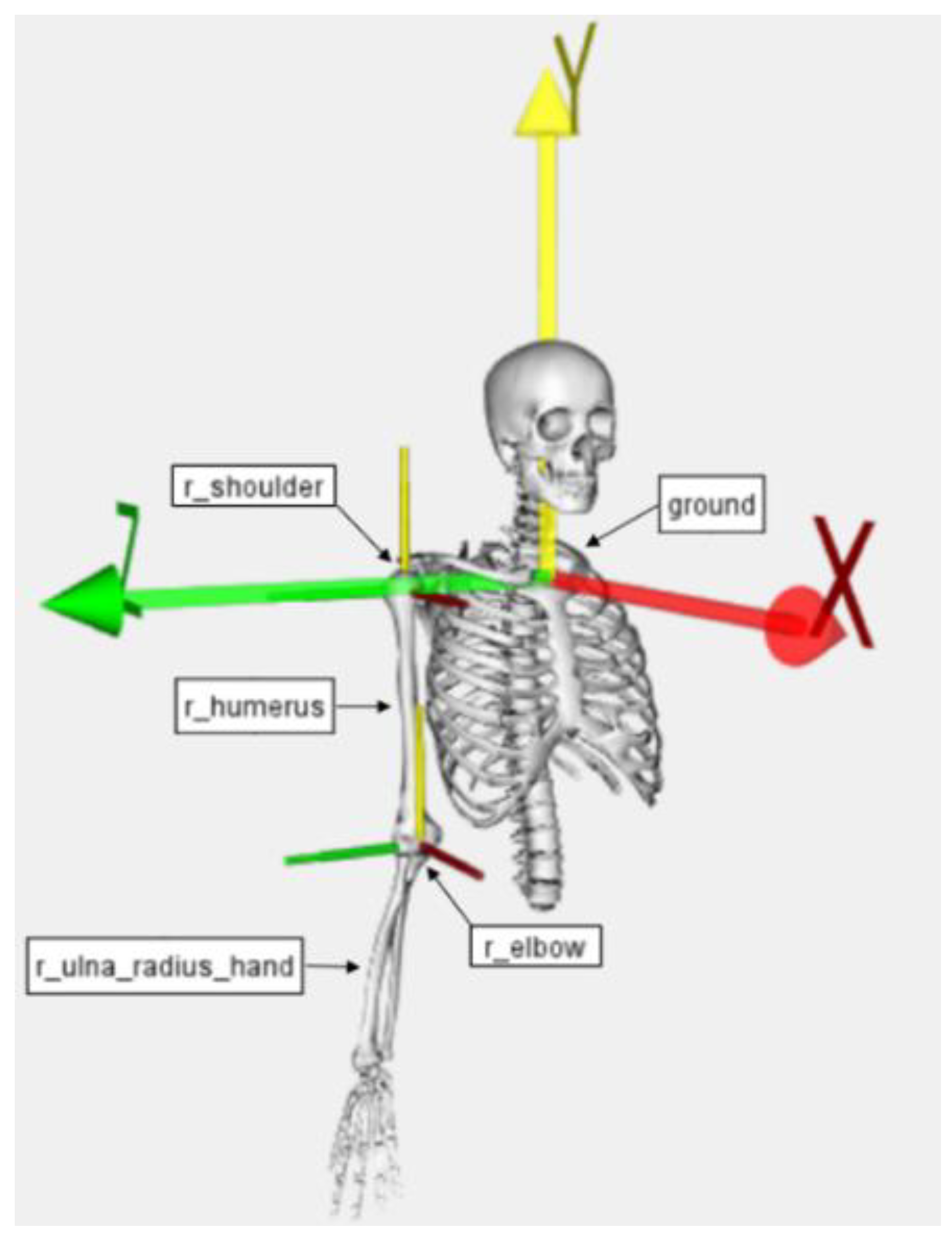
In this section, the results regarding the simulation of the upper limb subjected to gravity during a simple kinematics are discussed. The input data are taken from the OpenSim model “arm26” [22]. As already mentioned, the analysed upper limb is composed of three bodies: ground, humerus and forearm; these are linked by two revolute joints, the shoulder and elbow, whose main data (inertial properties, relative locations and rotation axes) are listed in

Table 1. Bodies’ inertial properties.

Body	$\mathbf{Mass} \mathit{m} \left[\mathrm{kg}\right]$	Inertia Tensor Entries
		${\overline{\mathit{I}}}_{\mathit{x}\mathit{x}} \left[g m^2\right]$	${\overline{\mathit{I}}}_{\mathit{y}\mathit{y}} \left[g m^2\right]$	${\overline{\mathit{I}}}_{\mathit{z}\mathit{z}} \left[g m^2\right]$	${\overline{\mathit{I}}}_{\mathit{x}\mathit{y}} \left[g m^2\right]$	${\overline{\mathit{I}}}_{\mathit{y}\mathit{z}} \left[g m^2\right]$	${\overline{\mathit{I}}}_{\mathit{x}\mathit{z}} \left[g m^2\right]$
Humerus	1.86	14.81	4.55	13.19	0	0	0
Forearm	1.53	19.28	1.57	20.06	0	0	0

,

Table 2. Bodies’ mass center position with respect to the reference joints.

Body	Local Position Vector
	${\overline{\mathit{u}}}_{\mathit{G}\mathit{x}} \left[\mathit{m}\right]$	${\overline{\mathit{u}}}_{\mathit{G}\mathit{y}} \left[\mathit{m}\right]$	${\overline{\mathit{u}}}_{\mathit{G}\mathit{z}} \left[\mathit{m}\right]$
Humerus	0	−0.180	0
Forearm	0	−0.181	0

,

Table 3. Joints’ positions with respect to the reference joints.

Joint	Local Position Vector
	${\overline{\mathit{u}}}_{\mathit{J}\mathit{x}} \left[\mathit{m}\right]$	${\overline{\mathit{u}}}_{\mathit{J}\mathit{y}} \left[\mathit{m}\right]$	${\overline{\mathit{u}}}_{\mathit{J}\mathit{z}} \left[\mathit{m}\right]$
Shoulder	−0.0175	−0.0070	0.1700
Elbow	0.0061	−0.2904	−0.0123

and

Table 4. Joints’ rotation axed with respect to the parent bodies.

Joint	Unit Vector Axis
	${\widehat{\mathit{v}}}_{\mathit{x}}$	${\widehat{\mathit{v}}}_{\mathit{y}}$	${\widehat{\mathit{v}}}_{\mathit{z}}$
Shoulder	−0.0589	0.0023	0.9983
Elbow	0.0494	0.0366	0.9981

.

The musculoskeletal system is moved by six muscles (long triceps, lateral triceps, medial triceps, long biceps, short biceps and brachialis), characterised by parameters included in the

Table 5. Muscles’ properties.

Muscle	Maximum Isometric Force ${\mathit{F}}_0 \left[\mathit{N}\right]$	Optimal Muscle Fibre Length ${\mathit{l}}_0 \left[\mathit{m}\right]$	Slack Tendon Length ${\mathit{l}}_{\mathit{t}} \left[\mathit{m}\right]$	Optimal Pennation Angle ${\mathit{\alpha }}_0 \left[\mathit{r}\mathit{a}\mathit{d}\right]$	Maximum Contraction Velocity ${\mathit{v}}_{\mathit{m}\mathit{a}\mathit{x}} \left[{\mathit{l}}_0/\mathit{s}\right]$
Long triceps	798.52	0.1340	0.1430	0.209	10
Lateral triceps	624.30	0.1138	0.0980	0.157	10
Medial triceps	624.30	0.1138	0.0908	0.157	10
Long biceps	624.30	0.1157	0.2723	0	10
Short biceps	435.56	0.1321	0.1923	0	10
Brachialis	987.26	0.0858	0.0535	0	10

.

The wrapping surfaces included are a cylinder fixed to the ground interacting with the long triceps, a first ellipsoid interacting with the long biceps, a second ellipsoid interacting with the long triceps (both the ellipsoids are fixed to the humerus) and a cylinder fixed to the humerus interacting with all the triceps on the back and with the brachialis on the front. The wrapping surfaces have locations ${\overline{\mathit{u}}}_w$ and orientations ${\mathit{\theta }}_w$ with respect to the reference joints, these are reported in

Table 6. Wrapping surfaces location and orientation with respect to the reference joints and geometry.

Wrapping Surface	Local Position Vector			Local Orientation			Geometry
	${\overline{\mathit{u}}}_{\mathit{w},\mathit{x}} \left[\mathit{m}\right]$	${\overline{\mathit{u}}}_{\mathit{w},\mathit{y}} \left[\mathit{m}\right]$	${\overline{\mathit{u}}}_{\mathit{w},\mathit{z}} \left[\mathit{m}\right]$	${\mathit{\theta }}_{\mathit{w},\mathit{x}} \left[\mathit{r}\mathit{a}\mathit{d}\right]$	${\mathit{\theta }}_{\mathit{w},\mathit{y}} \left[\mathit{r}\mathit{a}\mathit{d}\right]$	${\mathit{\theta }}_{\mathit{w},\mathit{z}} \left[\mathit{r}\mathit{a}\mathit{d}\right]$	$\left[\mathit{m}\mathit{m}\right]$
Ground cylinder	−0.0439	−0.0039	0.1478	1.3753	−0.2946	2.4360	$\begin{array}{c}r=3\\ h=30\end{array}$
Shoulder ellipsoid 1	−0.0078	−0.0041	−0.0014	3.0016	−0.8535	2.5742	$\begin{array}{c}{s}_x=35\\ s_y=20\\ s_z=20\end{array}$
Shoulder ellipsoid 2	0.0033	0.0073	0.0003	−2.0043	−1.0016	0.9755	$\begin{array}{c}{s}_x=25\\ s_y=20\\ s_z=20\end{array}$
Elbow cylinder	0.0028	−0.2919	−0.0069	−0.1402	−0.0063	0.1550	$\begin{array}{c}r=16\\ h=50\end{array}$

, along with the surface geometries.

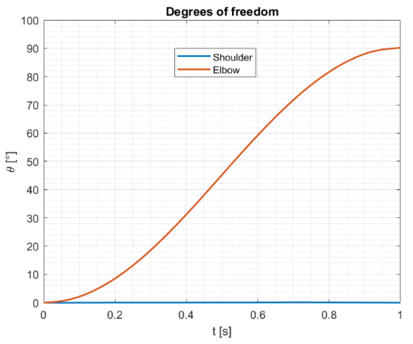
The degrees of freedom are the shoulder and the elbow rotations and the analysed kinematics, as reported in Figure 7, which shows the movement of the elbow from 0° to 90° during 1 s while the shoulder does not move.

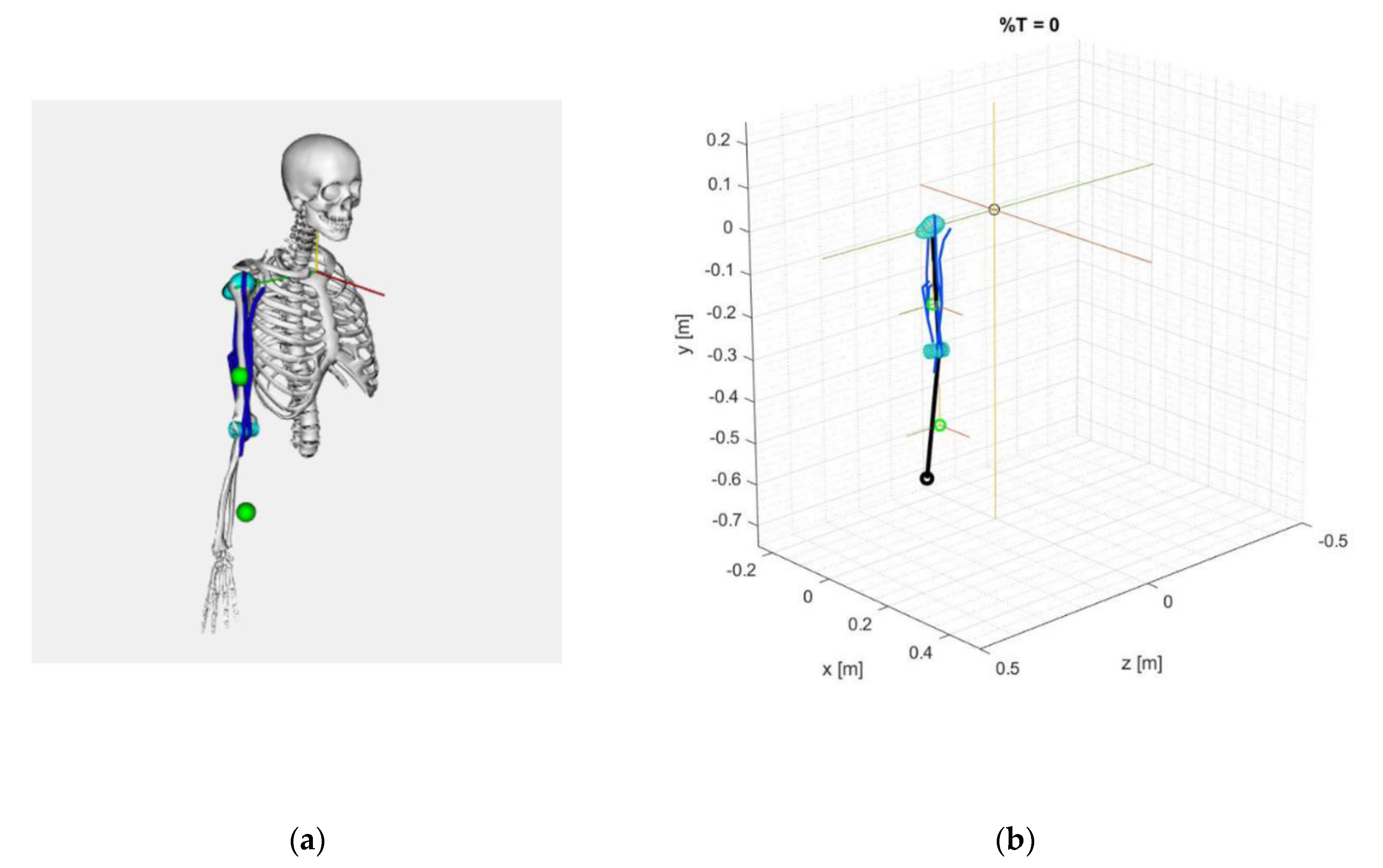
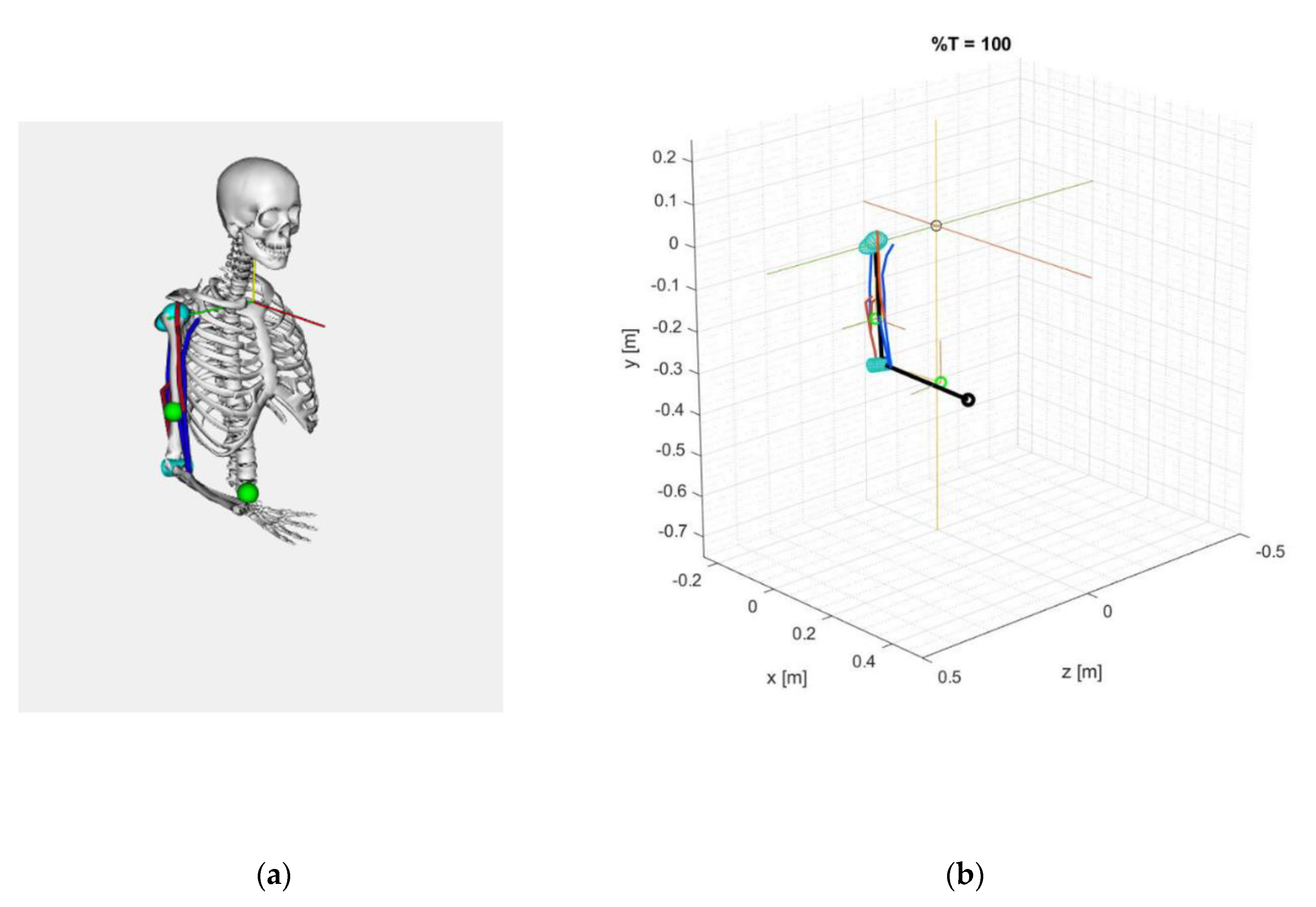
In order to prove the reliability of the kinematical analysis, Figure 8; Figure 9 show the comparison between the system configuration (the position of the bodies with their mass centre, the muscles and the wrapping surfaces) in the OpenSim model and in the Matlab model, in correspondence of the first and the last time instants. The kinematical analysis can be viewed in Supplementary Materials—Video S1.

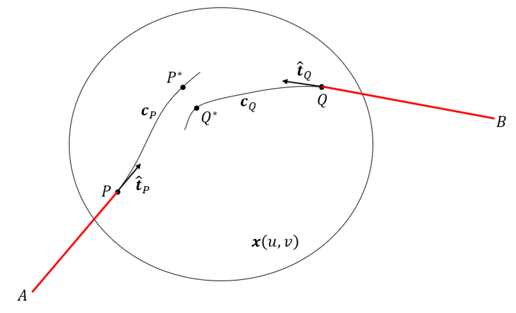
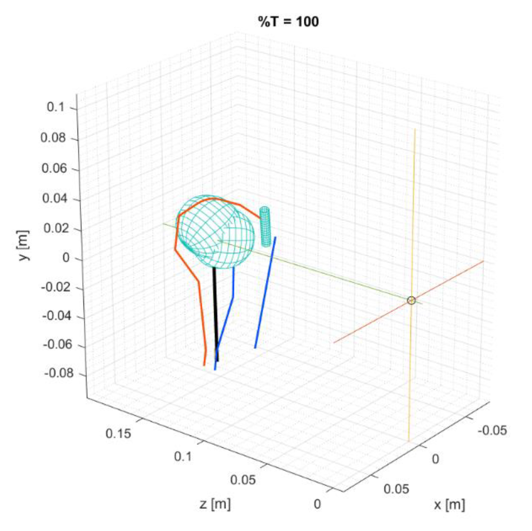
The long biceps wrapped on the ellipsoid keeps its path on the surface during the simulation because the shoulder angle is constant; it is shown in Figure 10.

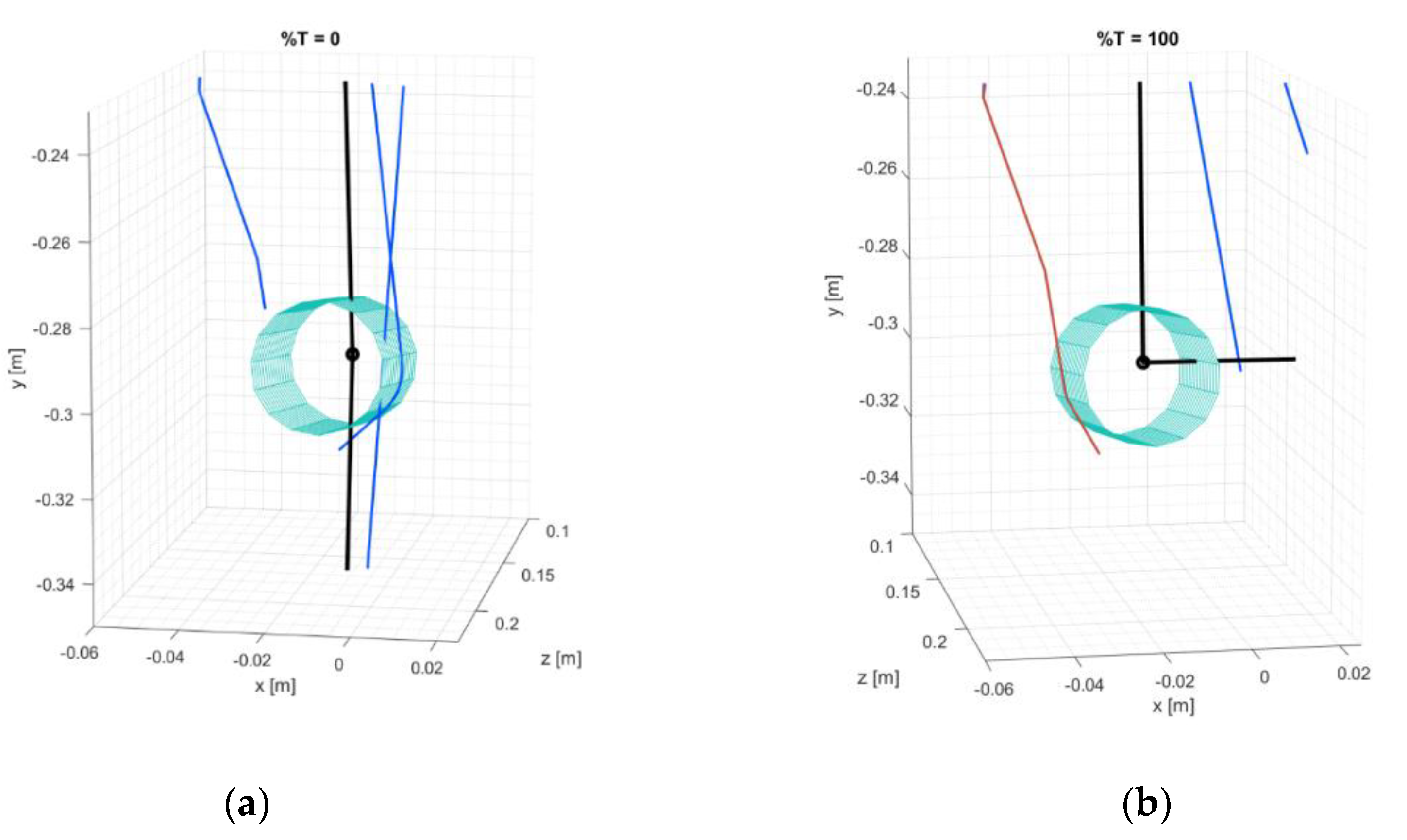
The wrapping muscles on the cylinder close to the elbow are viewed in Figure 11 at the start and at the end of the analysis time period, in order to show the brachialis wrapping on the cylinder front and the triceps wrapping on the cylinder back. The complete time evolution of the muscles’ wrapping on the cylinder is available in Supplementary Materials—Video S2.

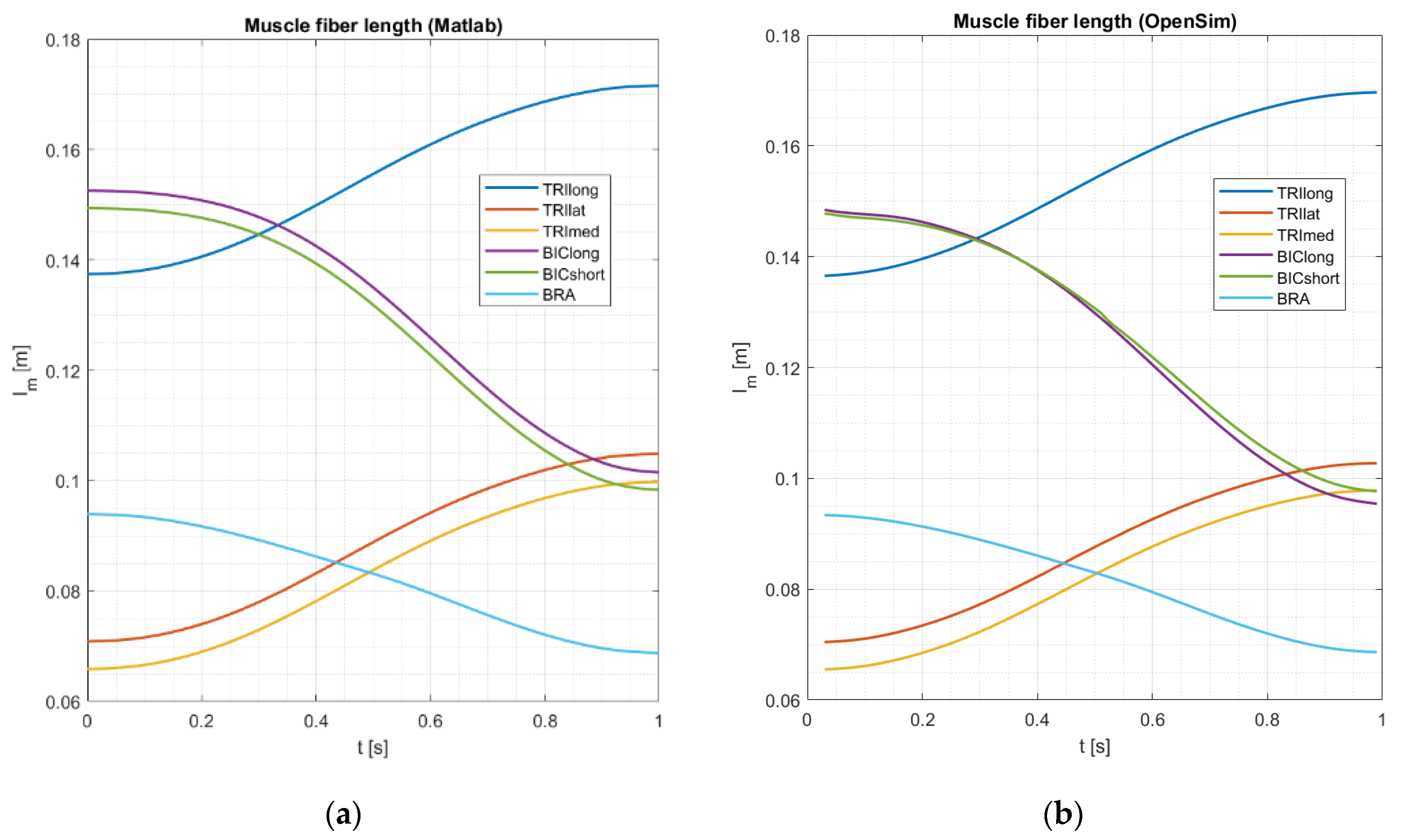
A first quantitative comparison in the framework of the kinematical analysis is shown in Figure 12 on the muscles’ fibre length $l_m$, which also accounts for the muscle wrapping.

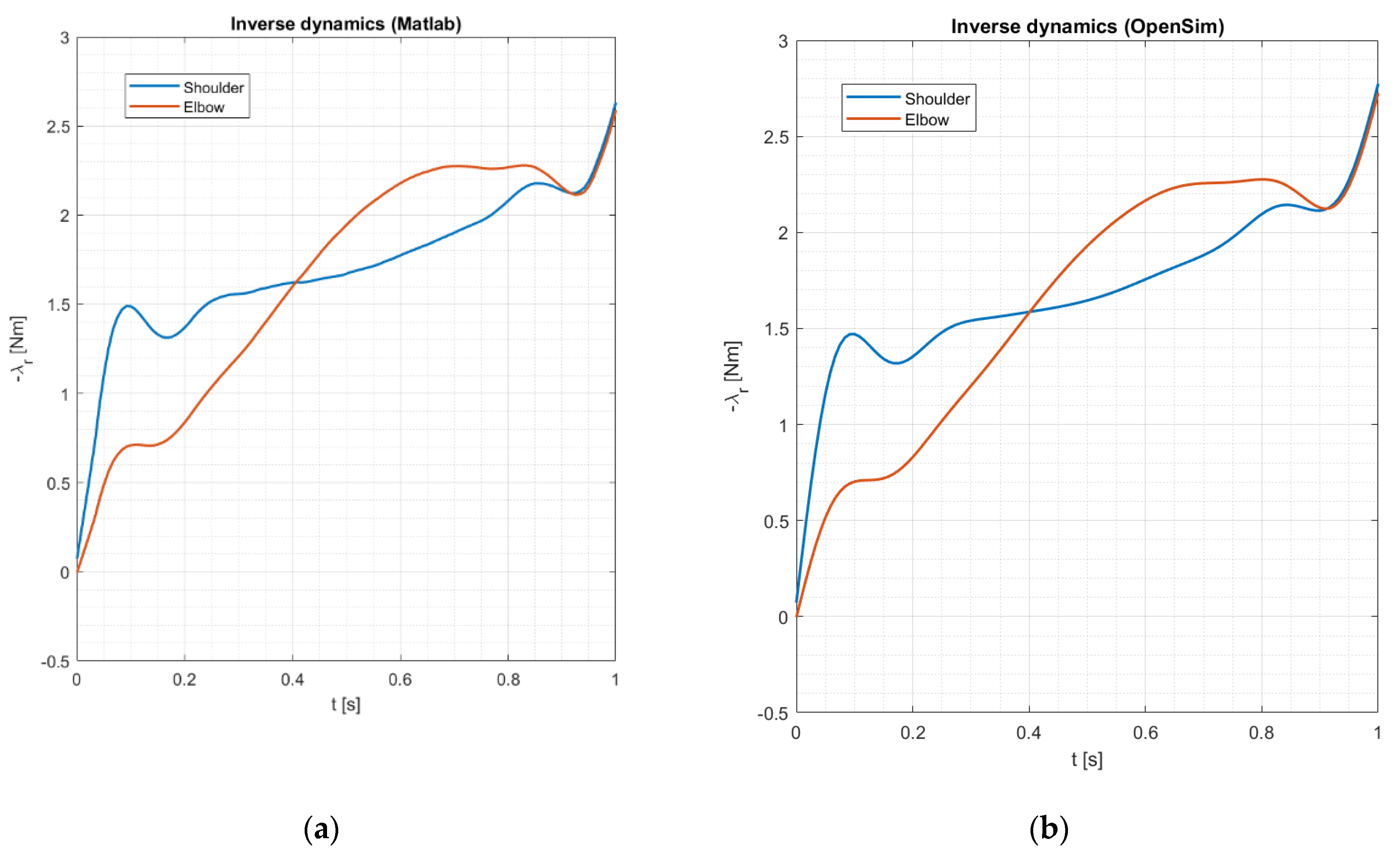
Given that the comparison is satisfactory, the unique noticeable difference is related to the long biceps fibre length, probably due to a different wrapping algorithm used by the OpenSim software. After the kinematical analysis, the results of the inverse dynamics are shown in the Figure 13, in which the comparison between OpenSim and Matlab is made on the driving forces (rheonomic Lagrange multipliers ${\lambda }_r$). The inverse dynamics outputs result in a very satisfactory match between the Matlab model and the OpenSim software.

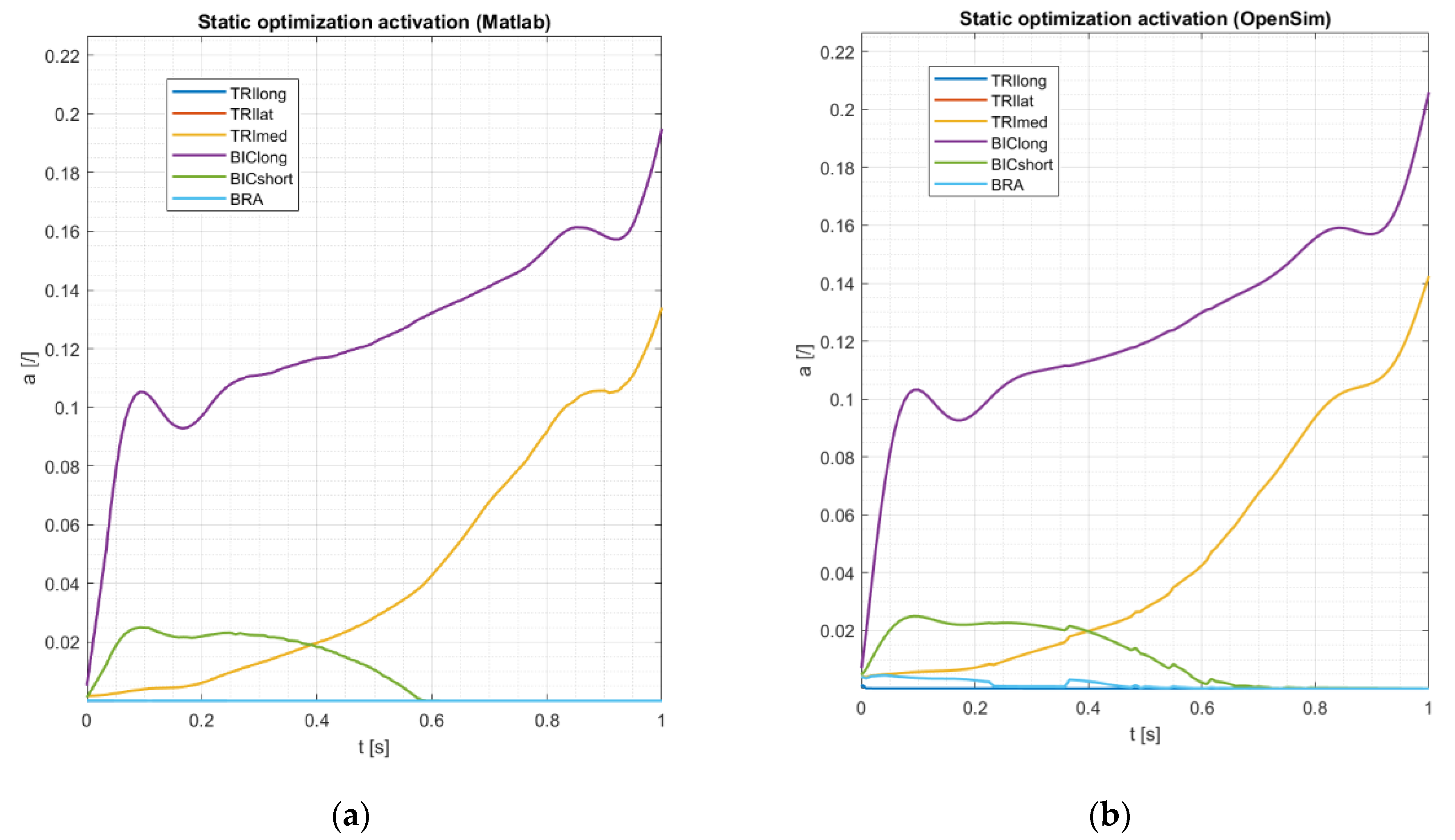
The tool “Static Optimization” in OpenSim does not take into account the muscle passive force and allows choosing between the physiological criterion by using the muscle’s force–length–velocity relationships or not. In the latter option the muscular activation $a$ is intended as the ratio between the muscle force $F_m$ and the maximum isometric force $F_0$, bounded between 0 and 1. In the configuration of non-physiological criterion, the comparison on the muscles’ activation is shown, respectively, in Figure 14. The comparison of the muscle forces is not shown because in this case the forces are proportional to the activations. The evaluated activations $a$ calculated with the Matlab model are slightly underestimated with respect to the ones evaluated by OpenSim, which, moreover, show some discontinuities.

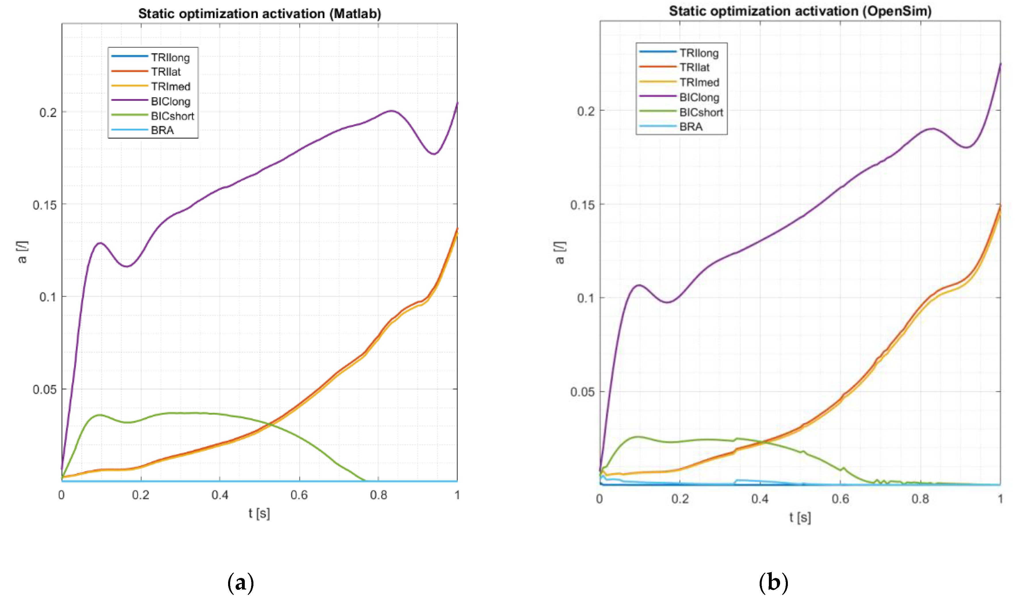
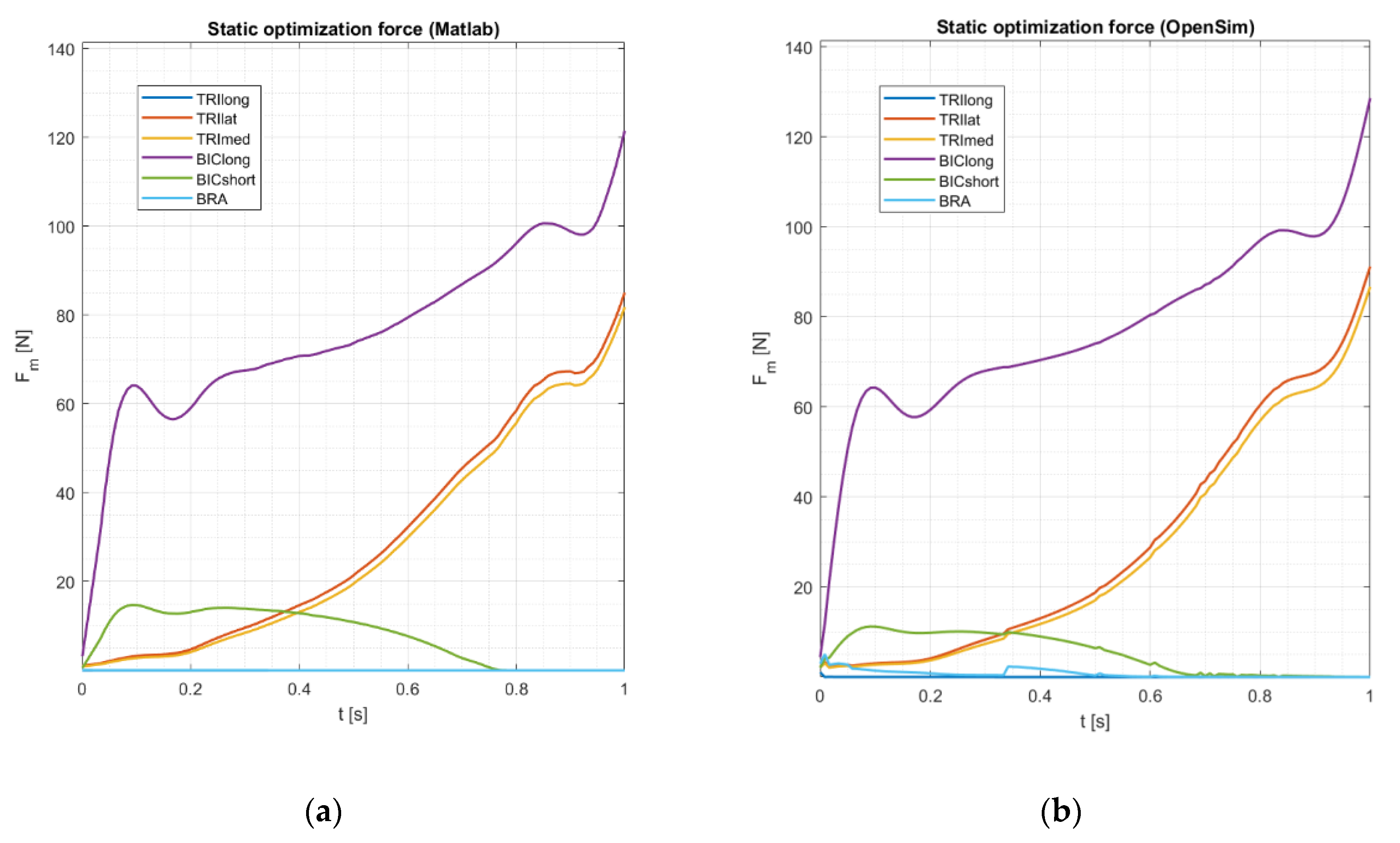
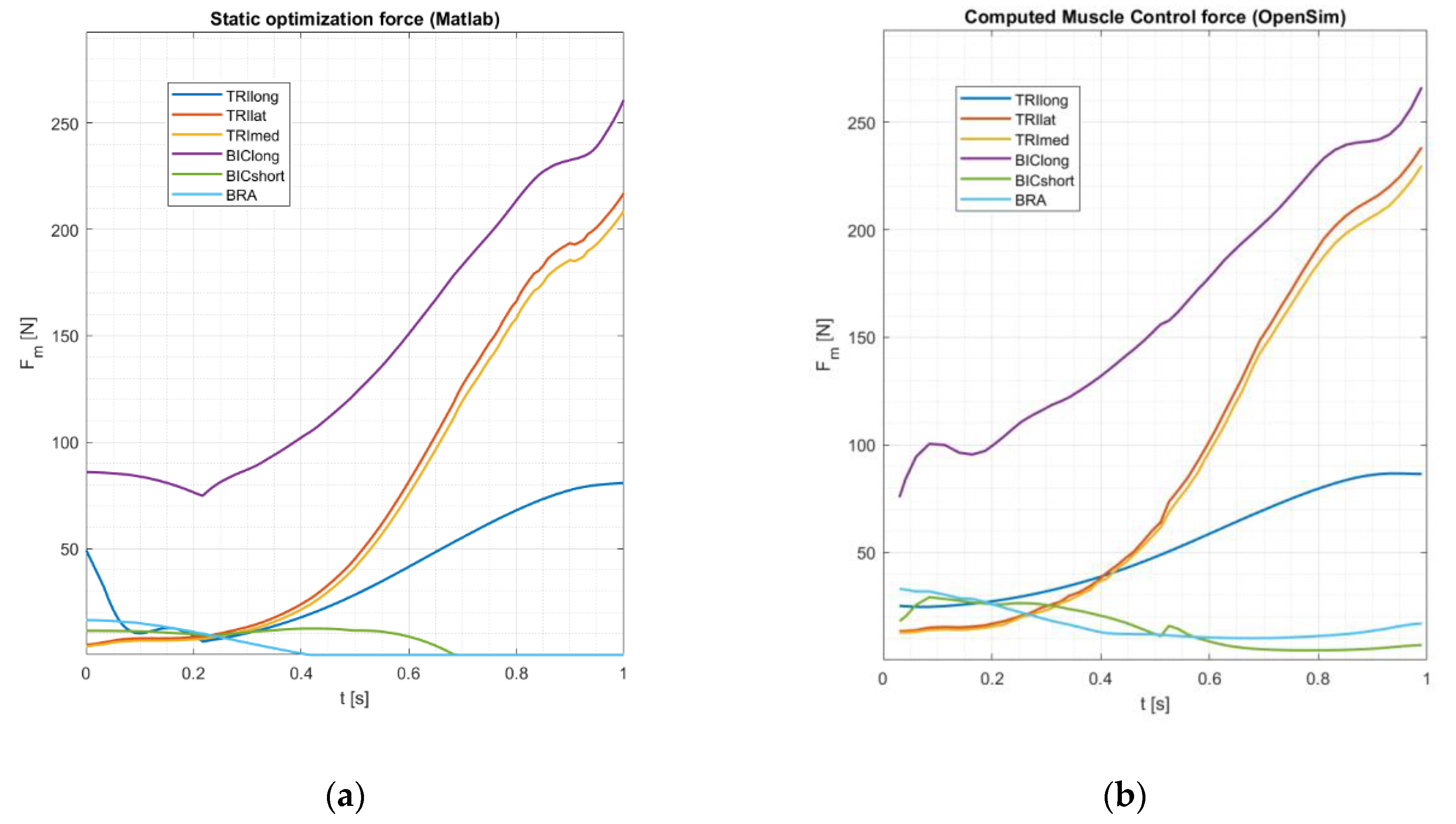
The results obtained with the physiological criterion but not taking into account the passive muscle forces are shown in Figure 15, in terms of muscle activations $a$, and in Figure 16, in terms of muscle forces $F_m$. In this configuration there are small underestimations and overestimations in different parts of the time period and the OpenSim software returns some discontinuities, regarding both the activations and the muscle forces.

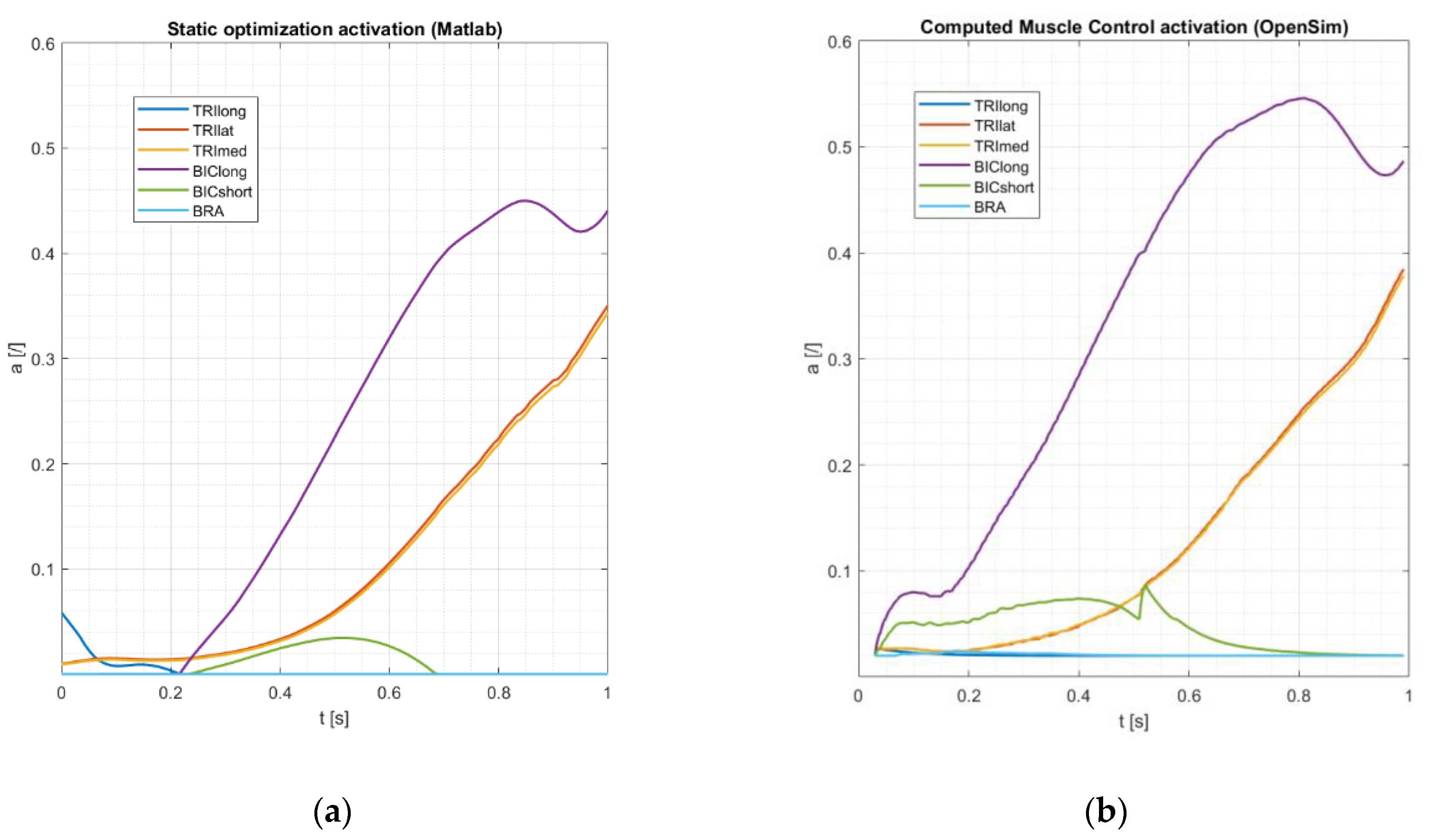
The “Computed Muscle Control” tool in OpenSim [36] allows evaluating the muscle activations, also considering the passive muscle forces, by calculating through PID controllers the muscle actions necessary to obtain the minimum difference between the trajectories of the degrees of freedom simulated with the forward dynamics and the ones known by inverse kinematics. The comparison results regarding the muscle activation $a$ and the muscle forces $F_m$ are shown respectively in Figure 17 and in Figure 18. In this last configuration, which includes all the analysed phenomena, despite the good qualitative match between the Matlab model and the OpenSim software, there are some discrepancies, probably due to the different approaches with respect to static optimization. While the muscle activations are underestimated, the muscle forces seems to be more similar to each other, except for the first instants of the time period discussed.

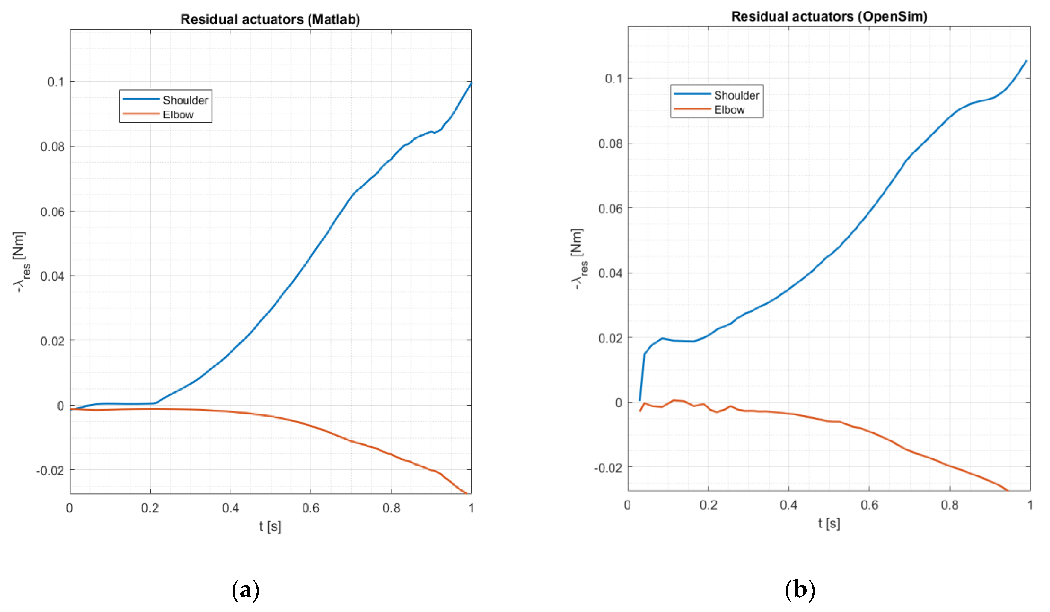
Another interesting result is obtained regarding the residual actuators ${\lambda }_{res}$ (which are the rheonomic Lagrange multipliers ${\lambda }_r$ of Equation (33)), also provided in the OpenSim tools, in this configuration. With reference to Figure 19, the residual actuators show a similar behaviour, both quantitively and qualitatively. The quantitative response of the residual actuators shows that the particular muscles’ topology, together with their characteristic parameters listed in Table 5, does not fully satisfy the equation of motion, since they result from the minimization, but their role is marginal if compared to the rheonomic Lagrange multipliers coming from the inverse dynamics (Figure 13) and, in fact, the residual action is needed just to reach the minimization convergence and to complete the calculus, not for substituting the real actuators represented by the muscles.

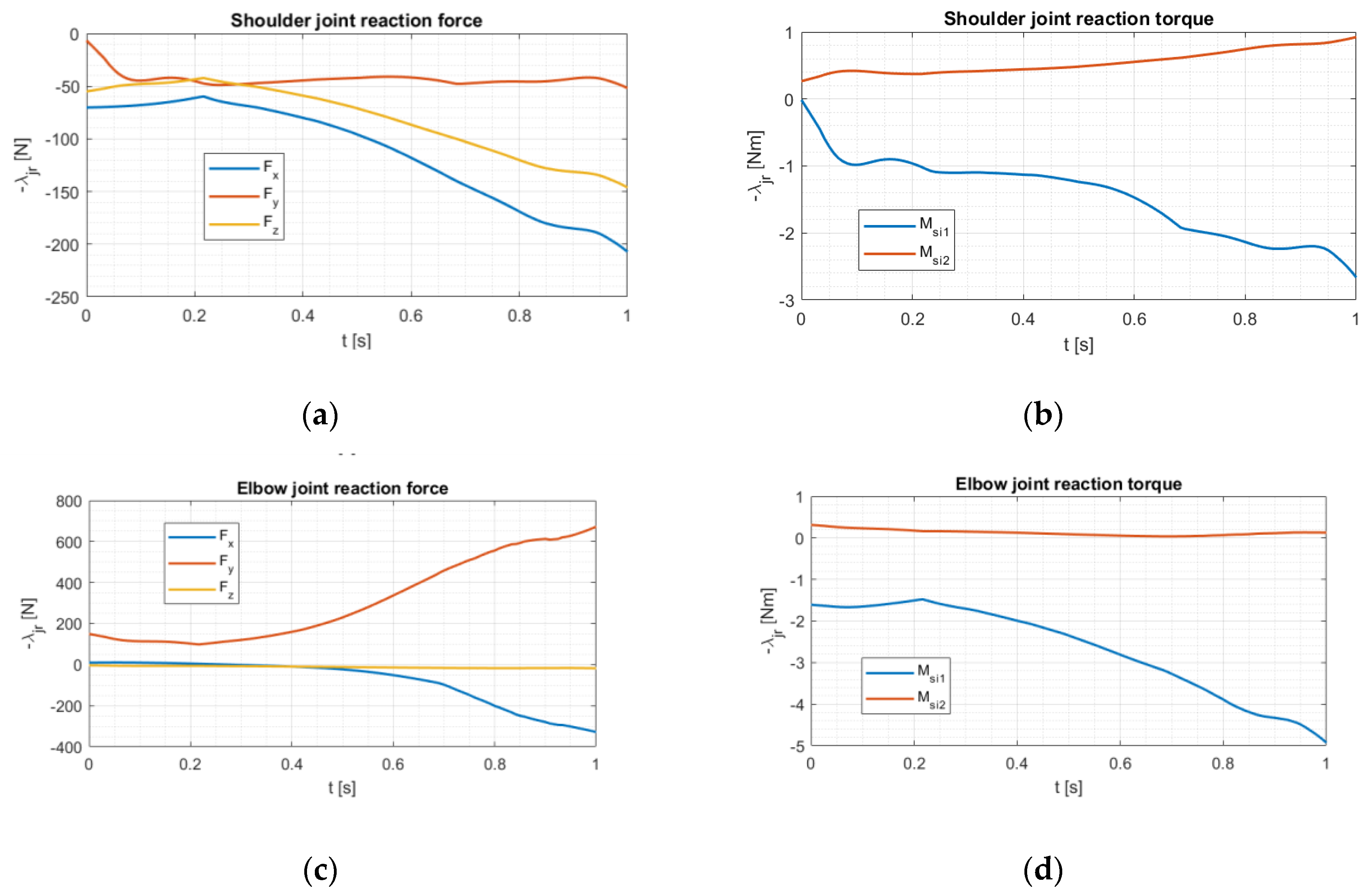
Once the inverse dynamics problem of the musculoskeletal system is solved, the Matlab model provides the joint reactions. In Figure 20, the joint reactions ${\lambda }_{jr}$ (which are the scleronomic Lagrange multipliers ${\lambda }_s$ of Equation (33)) which act on the upper limb joints during the analysed kinematics are shown.

4. Conclusions

The objective of this work was to propose and to describe step by step the procedure to achieve a general multibody approach able to solve the inverse dynamics problem of a musculoskeletal system, the upper limb, implemented in a novel code developed in the Matlab environment. By knowledge of the musculoskeletal system degrees of freedom together with the system’s topology, the model allows a kinematical analysis based on the evaluation of the constraints’ kinematical behaviour. Subsequently, associating an actuator for each degree of freedom and including the external forces, the inverse dynamics is solved by calculating the rheonomic Lagrange multipliers, related to the driving actions that lead the system to move following the known kinematics. The knowledge of the muscles’ topology leads the kinematical analysis to evaluate the muscle paths between the bodies and around the wrapping surfaces fixed to the bodies: in the case of wrapped muscle, an algorithm based on the calculus of geodesic curves is used. The muscle paths are involved in the elaboration of the muscles’ lengths, deformation velocities and pennation angles, in order to include in the equation of motion, through the Hill muscle model, the muscles’ passive forces and the muscles’ activations. The last step of the model is to analyse the muscular recruitment through static optimization: the evaluation of the set of muscles’ activation levels and joint reaction forces, able to minimize the global activation and to satisfy the equation of motion.

The effectiveness of the model was examined by its application on an upper limb model subjected to a simple kinematics and to gravity forces. All the inputs data were taken from the OpenSim software and the simulation results were compared with the ones provided by the software, obtaining a general satisfactory qualitative and quantitative matching:

-

despite the kinematical analysis, exactness is noticeable, the only difference found was a small overestimation of the long biceps muscle fibre length, probably due to the different wrapping algorithm used by OpenSim;

-

the inverse dynamics in terms of driving force results were almost completely matched;

-

the static optimization was characterised by a general underestimation of the muscles’ activations in all the cases considered (both physiological and non-physiological criterion in absence of passive muscles’ forces and physiological criterion considering the passive muscle actions compared with the Computed Muscle Control tool of OpenSim). The underestimation was regained by comparing the muscle forces, the differences were probably due to the different approaches in the minimization techniques and, certainly, to the different approach to the inverse dynamics of the Computed Muscle Control;

-

the good outcome of the comparison was also confirmed by the matching of the residual actuators.

In summary, with the limitation of its validation with only one imposed upper limb kinematics, the model resulted as a suitable, open and fully controllable tool in the framework of the multibody musculoskeletal dynamics of the human upper limb. However, despite the model being characterised by the accurate analytical description of important muscular phenomena (muscle dynamics, recruitment and wrapping), it has to process more complex kinematics in order to perform a more accurate validation and to design a fully in silico optimization model of the artificial human joints. The deepening of the involved phenomena is always a stimulating necessity, in order to understand more clearly the human body mechanical behaviour, so future research perspectives will be devoted to:

-

a full validation with more upper limb kinematics;

-

the application of the model in the framework of the lower limb musculoskeletal system, in order to compare the simulated joint reactions with the in vivo measurements during the gait analysis;

-

the coupling of the model with a lubrication one, in order to estimate the wear of an artificial joint or to evaluate the joints friction forces or torques to include in the equation of motion as non-conservative actions;

-

the upgrade of the model by including the forward dynamics, in order to make a detailed comparison with the Computed Muscle Control tool of the OpenSim software;

-

the deepening of the Hill muscle model, in order to include the tendon dynamics;

-

the possible applications of the model in the framework of the biomechatronics and robotics fields.

References

1. Ruggiero, A.; Sicilia, A. A Mixed Elasto-Hydrodynamic Lubrication Model for Wear Calculation in Artificial Hip Joints. Lubricants 2020, 8, 72. [Google Scholar] [CrossRef]
2. Ruggiero, A.; Sicilia, A. Lubrication modeling and wear calculation in artificial hip joint during the gait. Tribol. Int. 2020, 142, 105993. [Google Scholar] [CrossRef]
3. Ruggiero, A.; Sicilia, A.; Affatato, S. In silico total hip replacement wear testing in the framework of ISO 14242-3 accounting for mixed elasto-hydrodynamic lubrication effects. Wear 2020, 460, 203420. [Google Scholar] [CrossRef]
4. Chen, Z.; Chen, Z.; Xin, H.; Zhang, Q.; Jin, Z. Musculoskeletal multibody dynamics simulation of the contact mechanics and kinematics of a natural knee joint during a walking cycle. Proc. Inst. Mech. Eng. Part H J. Eng. Med. 2018, 232, 508–519. [Google Scholar]
5. Varady, P.A.; Glitsch, U.; Augat, P. Loads in the hip joint during physically demanding occupational tasks: A motion analysis study. J. Biomech. 2015, 48, 3227–3233. [Google Scholar] [CrossRef]
6. Quental, C.; Folgado, J.; Ambrósio, J.; Monteiro, J. Multibody System of the Upper Limb Including a Reverse Shoulder Prosthesis. J. Biomech. Eng. 2013, 135, 111005. [Google Scholar] [CrossRef]
7. Stylianou, A.P.; Guess, T.M.; Kia, M. Multibody Muscle Driven Model of an Instrumented Prosthetic Knee During Squat and Toe Rise Motions. J. Biomech. Eng. 2013, 135, 41008. [Google Scholar] [CrossRef] [Green Version]
8. Ruggiero, A.; Merola, M.; Affatato, S. On the biotribology of total knee replacement: A new roughness measurements protocol on in vivo condyles considering the dynamic loading from musculoskeletal multibody model. Measurement 2017, 112, 22–28. [Google Scholar] [CrossRef]
9. Schwarze, M.; Hurschler, C.; Seehaus, F.; Oehler, S.; Welke, B. Loads on the prosthesis–socket interface of above-knee amputees during normal gait: Validation of a multi-body simulation. J. Biomech. 2013, 46, 1201–1206. [Google Scholar] [CrossRef] [PubMed]
10. Ruggiero, A.; Merola, M.; Affatato, S. Finite element simulations of hard-on-soft hip joint prosthesis accounting for dynamic loads calculated from a musculoskeletal model during walking. Materials 2018, 11, 574. [Google Scholar] [CrossRef] [Green Version]
11. Cosenza, C.; Niola, V.; Savino, S. A mechanical hand for prosthetic applications: Multibody model and contact simulation. Proc. Inst. Mech. Eng. Part H J. Eng. Med. 2018, 232, 819–825. [Google Scholar] [CrossRef] [PubMed]
12. Bergmann, G.; Bender, A.; Dymke, J.; Duda, G.; Damm, P. Standardized Loads Acting in Hip Implants. PLoS ONE 2016, 11, e0155612. [Google Scholar] [CrossRef] [PubMed]
13. Kassi, J.-P.; Heller, M.O.; Stoeckle, U.; Perka, C.; Duda, G.N. Stair climbing is more critical than walking in pre-clinical assessment of primary stability in cementless THA in vitro. J. Biomech. 2005, 38, 1143–1154. [Google Scholar] [CrossRef] [PubMed]
14. Westerhoff, P.; Graichen, F.; Bender, A.; Halder, A.; Beier, A.; Rohlmann, A.; Bergmann, G. In vivo measurement of shoulder joint loads during activities of daily living. J. Biomech. 2009, 42, 1840–1849. [Google Scholar] [CrossRef]
15. Nordin, M.; Frankel, V.H. (Eds.) Basic Biomechanics of the Musculoskeletal System; Lippincott Williams & Wilkins: Filadelfia, PA, USA, 2001. [Google Scholar]
16. Trinler, U.; Baker, R. Estimated landmark calibration of biomechanical models for inverse kinematics. Med. Eng. Phys. 2018, 51, 79–83. [Google Scholar] [CrossRef]
17. Silva, M.T.; Pereira, A.F.; Martins, J. An efficient muscle fatigue model for forward and inverse dynamic analysis of human movements. Procedia IUTAM 2011, 2, 262–274. [Google Scholar] [CrossRef] [Green Version]
18. Silva, M.T.; Ambrósio, J. Solution of Redundant Muscle Forces in Human Locomotion with Multibody Dynamics and Optimization Tools. Mech. Based Des. Struct. Mach. 2003, 31, 381–411. [Google Scholar] [CrossRef]
19. Curtis, N. Craniofacial biomechanics: An overview of recent multibody modelling studies. J. Anat. 2010, 218, 16–25. [Google Scholar] [CrossRef]
20. Duprey, S.; Naaim, A.; Moissenet, F.; Begon, M.; Cheze, L. Kinematic models of the upper limb joints for multibody kinematics optimisation: An overview. J. Biomech. 2017, 62, 87–94. [Google Scholar] [CrossRef] [Green Version]
21. Huynh, K.; Gibson, I.; Jagdish, B.; Lu, W. Development and validation of a discretised multi-body spine model in LifeMOD for biodynamic behaviour simulation. Comput. Methods Biomech. Biomed. Eng. 2013, 18, 175–184. [Google Scholar] [CrossRef]
22. Holzbaur, K.R.S.; Murray, W.M.; Delp, S.L. A Model of the Upper Extremity for Simulating Musculoskeletal Surgery and Analyzing Neuromuscular Control. Ann. Biomed. Eng. 2005, 33, 829–840. [Google Scholar] [CrossRef]
23. Shabana, A. Dynamics of Multibody Systems; Cambridge University Press: Cambridge, UK, 2020. [Google Scholar]
24. Nikravesh, P.E.; Gim, G. Systematic Construction of the Equations of Motion for Multibody Systems Containing Closed Kinematic Loops. J. Mech. Des. 1993, 115, 143–149. [Google Scholar] [CrossRef]
25. Oliveira, H. Inverse Dynamic Analysis of the Human Locomotion Apparatus for Gait; Instituto Superior Técnico: Lisbon, Portugal, 2016. [Google Scholar]
26. Jovanovic, K.; Vranic, J.; Miljkovic, N. Hill’s and Huxley’s muscle models-tools for simulations in biomechanics. Serbian J. Electr. Eng. 2015, 12, 53–67. [Google Scholar] [CrossRef] [Green Version]
27. Millard, M.; Uchida, T.; Seth, A.; Delp, S.L. Flexing Computational Muscle: Modeling and Simulation of Musculotendon Dynamics. J. Biomech. Eng. 2013, 135, 021005. [Google Scholar] [CrossRef]
28. Romero, F.; Alonso, F.J. A comparison among different Hill-type contraction dynamics formulations for muscle force estimation. Mech. Sci. 2016, 7, 19–29. [Google Scholar] [CrossRef] [Green Version]
29. John, C. Complete Description of the Thelen 2003 Muscle Model; OpenSim: Stanford, CA, USA, 2011. [Google Scholar]
30. Thelen, D.G. Adjustment of Muscle Mechanics Model Parameters to Simulate Dynamic Contractions in Older Adults. J. Biomech. Eng. 2003, 125, 70–77. [Google Scholar] [CrossRef] [Green Version]
31. Hada, M.; Yamada, D.; Tsuji, T. An analysis of equivalent impedance characteristics by modeling the human musculoskeletal structure as a multibody system. In Proceedings of the ECCOMAS Thematic Conference, Milano, Italy, 25–28 June 2007; pp. 1–20. [Google Scholar]
32. Gao, F.; Damsgaard, M.; Rasmussen, J.; Christensen, S.T. Computational method for muscle-path representation in musculoskeletal models. Biol. Cybern. 2002, 87, 199–210. [Google Scholar] [CrossRef]
33. Zarifi, O.; Stavness, I. Muscle wrapping on arbitrary meshes with the heat method. Comput. Methods Biomech. Biomed. Eng. 2016, 20, 1–11. [Google Scholar] [CrossRef]
34. Stavness, I.; Sherman, M.; Delp, S. A General Approach to Muscle Wrapping over Multiple Surfaces; Stanford University: Stanford, CA, USA, 2012. [Google Scholar]
35. Scholz, A.; Stavness, I.; Sherman, M.A.; Delp, S.L.; Kecskeméthy, A. Improved Muscle Wrapping Algorithms Using Explicit Path-Error Jacobians. New Adv. Mech. Mach. Sci. 2013, 15, 395–403. [Google Scholar]
36. Thelen, D.G.; Anderson, F.C.; Delp, S.L. Generating dynamic simulations of movement using computed muscle control. J. Biomech. 2003, 36, 321–328. [Google Scholar] [CrossRef]
Figure 1. OpenSim arm26 model topology.
Applsci 10 07760 g001
Figure 2. Revolute joint scheme.
Applsci 10 07760 g002
Figure 3. Hill muscle scheme.
Applsci 10 07760 g003
Figure 4. Hill model force–length (a) and force-velocity (b) curves.
Applsci 10 07760 g004
Figure 5. Geodesics on a wrapping surface.
Applsci 10 07760 g005
Figure 6. Muscle series.
Applsci 10 07760 g006
Figure 7. Arm26 degrees of freedom over time.
Applsci 10 07760 g007
Figure 8. Kinematics first time instant in (a) OpenSim and (b) Matlab.
Applsci 10 07760 g008
Figure 9. Kinematics last time instant in (a) OpenSim and (b) Matlab.
Applsci 10 07760 g009
Figure 10. Shoulder wrapping.
Applsci 10 07760 g010
Figure 11. Elbow wrapping in the (a) first and (b) the last time instants.
Applsci 10 07760 g011
Figure 12. Muscles’ fiber lengths comparison: (a) Matlab (a) and (b) OpenSim.
Applsci 10 07760 g012
Figure 13. Inverse dynamics comparison: (a) Matlab and (b) OpenSim.
Applsci 10 07760 g013
Figure 14. Muscles’ activations with non-physiological criterion and no passive forces: (a) Matlab and (b) OpenSim.
Applsci 10 07760 g014
Figure 15. Muscles’ activations with physiological criterion and no passive forces: (a) Matlab and (b) OpenSim.
Applsci 10 07760 g015
Figure 16. Muscles’ forces with physiological criterion and no passive forces: (a) Matlab and (b) OpenSim.
Applsci 10 07760 g016
Figure 17. Muscles’ activations with physiological criterion and passive forces: (a) Matlab and (b) OpenSim.
Applsci 10 07760 g017
Figure 18. Muscles’ forces with physiological criterion and passive forces: (a) Matlab and (b) OpenSim.
Applsci 10 07760 g018
Figure 19. Residual actuators: (a) Matlab and (b) OpenSim.
Applsci 10 07760 g019
Figure 20. Upper limb joint reactions: (a) shoulder forces, and (b) torques, (c) elbow forces and (d) torques.
Applsci 10 07760 g020