Estimating Slump Flow and Compressive Strength of Self-Compacting Concrete Using Emotional Neural Networks

Abstract

The characteristics of fresh and hardened self-compacting concrete (SCC) are an essential requirement for construction projects. Moreover, the sensitivity of admixture contents of SCC in these properties is highly impacted by that cost. The current study investigates to estimate the slump-flow (S) and compressive strength (CS), as fresh and hardened properties of SCC, respectively. Four developed soft-computing approaches were proposed and compared, including the group method of data handling (GMDH), Minimax Probability Machine Regression (MPMR), emotional neural network (ENN), and hybrid artificial neural network-particle swarm optimization (ANN-PSO), to estimate the S and 28-day CS of SCC, which comprises fly ash (FA), silica fume (SF), and limestone powder (LP) as part of cement by mass in total powder content. In addition, the impact of eight admixture components is investigated and evaluated to assess the sensitivity of admixture contents for the modelling of S and CS of SCC. The results demonstrate that the performance prediction of ENN model is more significant than other models in estimating S and CS characteristics of SCC. The overall of Pearson correlation coefficient, r, and root mean square error (RMSE) of ENN model are 97.80% and 20.16 mm, respectively, for the S. These are 96.07% and 2.59 MPa, respectively, for the CS. Furthermore, the sensitivity of the powder content of fly ash is shown to have a high impact on the estimated S and CS values of SCC.

1. Introduction

Concrete workability and strength are essential characteristics that should be determined and used widely in construction projects [1,2,3]. Compressive strength (CS) of concrete denotes the level of uniaxial compressive stress, which refers to the concrete properties of concrete after hardening [1]. The workability of concrete is required for the handling and producing of concrete during the construction. While it affects the cost of construction finalization [1]. Herein, the slump-flow (S) test is one of the tests that almost uses to estimate the concrete workability. Herein, with increasing the engineering applications of concrete, the self-compacting concrete (SCC) is developing to use with easy replacement in a narrow spacing of steel of reinforcement concrete [2,4,5]. For that, both SCC characteristics, CS and S, should be accurately estimated.

Several studies have investigated the parameters that influence the CS and S values of conventional concrete [6], SCC [4] and high strength concrete (HSC) [7]. Gholhaki et al. [5] summarized the impact of admixture contents of SCC in that fresh and hardened properties. From their literature, it can be concluded that fly ash (FA), silica fume (SF), limestone powder (LP), metakaolin (MK) and water/powder (W/P) ratio are the main factors that can be impacted on the SCC properties. More explanation for the impact of admixture contents in the SCC characteristics can be found in [8,9,10]. However, the modeling approaches that can be used to estimate optimal admixture and SCC properties are still limited. Experimental design and regression models are usually utilized to determine the CS and S values of concrete [4,7].

Currently, different linear and nonlinear regression approaches have been utilized to estimate the SC and/or S values of concrete, including group method of data handling (GMDH), Minimax Probability Machine Regression (MPMR), emotional neural network (ENN), and artificial neural network (ANN). For instance, Dutta et al. [11] applied MPMR to predict the CS of concrete, and the results showed that the performance of it is acceptable, coefficient of correlation (R) = 93.5%, to use for estimating the CS values. Belalia-Douma et al. [12] used ANN to predict the S and CS of SCC, and authors concluded that the ANN is a useful method can be used into predicting SCC properties, with R = 80% and 95% for the S and CS, respectively. Fuzzy logic was also applied to estimate the S and CS of concrete and the results of it showed accurate with an acceptable rate of errors [6]. Deep learning based on ANN was also applied to estimate the S value of SCC, and the results showed the performance of the proposed model could be utilized routinely estimate SCC workability [13]. Biswas et al. [14] used ENN to estimate the CS of hardened concrete and the results showed it is robust for predicting of concrete behavior. GMDH was found a great tool can be applied to estimate the CS of hardened concrete and CS based on a core test of concrete [15,16]. More studies can be found in [1,2,3,4,11,17,18,19,20] for using advanced soft computing techniques into detecting the S and CS values of conventional concrete, SCC and HSC.

Furthermore, hybrid algorithms have been used to estimate concrete properties. Sadowski et al. [21] combined ANN with the imperialist competitive algorithm, and they found that that model is applicable to estimate the CS of conventional concrete. Shariati et al. [22] compared a hybrid artificial neural network–particle swarm optimization (ANN-PSO) with ANN to estimate the behavior of channel connectors in normal and HSC, and the performance of ANN-PSO was seen better. Optimization algorithm (WOA) was integrated with ANN to predict the CS of conventional concrete, and the results showed that integration was improved the modeling for CS values [23]. A combination between fuzzy radial basis based on ANN with biogeography-based optimization was proposed to estimate the CS of SCC and good performance of CS was obtained from the proposed model [24].

This study aims to design a novel model to be used to estimate the S and 28-day CS of SCC containing FA, SF, and LP based on its mix design, i.e., cement (C), FA, SF, LP, water (W), superplasticizer (SP), coarse aggregate (CG), fine aggregate (FG). Four models are evaluated and compared in the current study, including GMDH, MPMR, ENN, and ANN-PSO approaches. The proposed models are evaluated and assessed using experimental data of 90 different concrete mix-designs of SCC were obtained from Elemam et al. [4]. Based on our state-of-the-art research, the proposed models were not previously evaluated to estimate the CS and/or S of SCC with a different admixture containing FA, SF, and LP as part of cement by mass in total powder content. Furthermore, the sensitivity of the admixture contents was evaluated based on the obtained results of optimum proposed models.

2. Material and Methods

2.1. Dataset Employed

The admixture properties, materials and the detail of obtained datasets were given from Elemam et al. [4]. Here, a summary of the dataset used in this study was presented. The materials used to conduct SCC are ordinary Portland cement (C) CEMI 52.5 N; class F FA, SF, and LP were used as cementing and filler materials. The physical and chemical properties of C, FA, LP, SF are presented in

Table 1. Physical and chemical characteristics of (Cement)C, (fly ash) FA, (limestone powder) LP, and (silica fume) SF [4].

Oxide Composition	C	FA	LP	SF
CaO (%)	62.70	4.18	96.40	0.54
SiO2 (%)	20.20	52.00	-	90.20
Al2O3 (%)	6.00	21.54	-	0.45
Fe2O3 (%)	3.30	5.96	0.10	0.37
MgO (%)	2.00	1.05	2.31	4.26
SO3 (%)	2.20	0.37	-	0.32
Specific surface area (m2/kg)	360	420	535	23,530
Specific gravity	3.15	2.38	2.80	2.22

. SP of polycarboxylate, ASTM C494 Type F, was utilized in the admixture contents. The CG and FG were designed based on BS EN 12620, and that comprise a crushed dolomite size 12.5 mm and natural sand with 2.975 fineness modulus for the CG and FG, respectively [4].

The mix preparation was designed based on six independent variables that focused on the percentage of total powder (P) content of the admixture. FA, SF, and LP were replaced the cement by mass of total powered material. The percentage of FG/CG was selected constant for all cases. The control sample of SCC admixture was designed to attain 680 mm and 44.3 MPa for slump flow diameter and 28-day compressive strength, respectively; the mix ingredients of the control mixture is presented in

Table 2. Mixture contents of control (self-compacting concrete) SCC.

Item	Powder (kg/m3)	C (%)	FA (%)	LP (%)	SF (%)	W/P	SP (%)	Sand: Dolomite
content	500	65	20	10	5	0.38	1.15	1:1

[4]. The experimental preparation and tests were presented in Elemam et al. [4]; a cone (300 mm high, 100 mm and 200 mm of upper and lower diameters, respectively) was used to measure the slump flow, and a hydraulic machine test (capacity and accuracy 200 tons and 0.5 ton, respectively) was utilized to extract the compressive strength of 100 mm cubes after 28 days. The total number of experiments was calculated using an equation and designed codes ranges, more details can be found in Elemam et al. [4].

In the current study, eight variables are considered as input variables to estimate S and CS of SCC.

Table 3. Input and output variables range.

Variable	C (kg/m3)	FA (kg/m3)	LP (kg/m3)	SF (kg/m3)	W (kg/m3)	SP (kg/m3)	CG (kg/m3)	FG (kg/m3)	S (mm)	CS (MPa)
Average	325.00	100.00	50.00	25.00	190.01	6.25	816.66	816.66	708.28	41.31
Maximum	382.50	150.00	100.00	50.00	215.50	7.50	865.00	865.00	925.00	62.30
Minimum	270.60	50.00	0.00	0.00	165.00	5.00	768.30	768.30	400.00	20.90

illustrates the input and output variables range. From the table, it can be seen that there is a variety of range in the input variables; the maximum ranges were observed in the powered contents, C, FA, LP, and SF. This means that the powdered contents are a significant function that could be affected the SCC properties, S and CS, besides the main variables of concrete, W, CG, and FG.

The datasets were randomly divided into three data phases to carry out the proposed models:

(a)

Training phase: Included the required data for the design of the proposed models. Sixty-three out of 90 (70%) datasets were used as the training phase.

(b)

Testing phase: Included the remaining data (30%) to evaluate the performance of the proposed models with an independent dataset.

(c)

Validation phase: Here, all the data (90 datasets) was used to qualify a model’s performance with a large amount of dataset.

2.2. Models Design and Evaluation

Four models were developed and evaluated in this study to estimate S and CS of SCC. The following are the algorithm summary of each model and the design models for detecting S and CS of SCC. The models were designed based on the multi-input single-output processing system.

2.2.1. GMDH Model

The GMDH is a self-organizing and complex approach through a complicated process by building a feed-forward network (FFN) function [15,16,25]. Although the GMDH has the same processing of ANN, it possesses some advantages compared by ANN, such as high speed and easier mathematical functions [25]. The current study developed GMDH model for estimating S and CS of SCC using eight input variables through a partial quadratic polynomials system.

In general, the relationship between inputs and output variables can be represented as follows [16]:

$$y=b_0+{\displaystyle \sum }_1^n{b}_i{x}_i+{\displaystyle \sum }_1^n{\displaystyle \sum }_1^n{b}_{ij}{x}_i{x}_j+{\displaystyle \sum }_1^n{\displaystyle \sum }_1^n{\displaystyle \sum }_1^n{b}_{ijk}{x}_i{x}_j{x}_k+\cdots$$

(1)

where, y and x represent the output and input variables, respectively, n is the number of observations for each variable, and b notes model coefficients.

Simply, a partial quadratic polynomials system for two inputs variables can be expressed as follows [15,16]:

$$y\left(x_i,x_j\right)=b_0+b_1{x}_i+b_2{x}_j+b_3{x}_i{x}_j+b_4{x}_i^2+b_5{x}_j^2$$

(2)

The least-square technique is used to calculate the model coefficients. $\left(\begin{array}{c}n\\ 2\end{array}\right)=\frac{n\left(n-1\right)}{2}$ neurons can be generated in the first hidden layer of the FFN from the measurements $\left\{\left(y_i,x_{ip},x_{iq}\right)(i=1,2,\dots ,M\right\}$ for different $p,q\in \left\{1,2,\dots ,n\right\}$ [1,15,16,25]. As a step for finding the unknown coefficients of the model, the inputs and output variables can be reconstructed in the following form.

$$\left[\begin{array}{cc}\begin{array}{cc}{x}_{1p}& x_{1q}\\ \begin{array}{c}{x}_{2p}\\ \begin{array}{c}⋮\\ x_{Mp}\end{array}\end{array}& \begin{array}{c}{x}_{2q}\\ \begin{array}{c}⋮\\ x_{Mq}\end{array}\end{array}\end{array}& \begin{array}{cc}\begin{array}{c}\dots \\ \begin{array}{c}\dots \\ \begin{array}{c}⋮\\ \dots \end{array}\end{array}\end{array}& \begin{array}{c}\begin{array}{c}{y}_1\\ y_2\end{array}\\ \begin{array}{c}⋮\\ y_M\end{array}\end{array}\end{array}\end{array}\right]$$

The quadratic sub-expression in Equation (2) use for each row of M to express the following matrix equation:

$$Y=Ab$$

(3)

where, b is the vector of model coefficients of quadratic polynomial and Y is the output vector. While matrix A can be expressed as follows, in the state of Equation (2), as an example:

$$A=\left[\begin{array}{cccccc}1& x_{1p}& x_{1q}& x_{1p}{x}_{1q}& x_{1p}^2& x_{1q}^2\\ 1& x_{2p}& x_{2q}& x_{2p}{x}_{2q}& x_{2p}^2& x_{2q}^2\\ \dots & \dots & \dots & \dots & \dots & \dots \\ 1& x_{Mp}& x_{Mq}& x_{Mp}{x}_{Mq}& x_{Mp}^2& x_{Mq}^2\end{array}\right]$$

(4)

Therefore, based on the least-square method, the unknown coefficients can be obtained as follows:

$$b={\left(A^{T}A\right)}^{-1}{A}^{T}Y$$

(5)

In this method, the connectivity topology of the network design based on three parameters, that are maximum neuron numbers (Nn), the maximum number of layers (Ln), and selection-pressure criteria (α) [25]. The Nn can be calculated using $\left(\begin{array}{c}n\\ 2\end{array}\right)=\frac{n\left(n-1\right)}{2}$ formula. While, the Ln and α can be estimated based on the best determination of root mean square error (RMSE) and Pearson correlation coefficient (r) for the neurons; meanwhile, the network scheme was also designed based on the RMSE values, based on the best or worst RMSE, the neurons can be removed or accepted using RMSE and r values. More details for the estimating of these parameters can be found in et al. [25]. In this study, the best models for S and CS of SCC were generated and concluded in

Table 4. GMDH model parameters for S and CS of CSS.

Model Parameters	Nn	Ln	α
S	15	5	0.3
CS	10	4	0.3

.

2.2.2. MPMR Model

The MPMR theory was presented and applied in [11,26,27,28]. In general, MPMR is a kernel regression algorithm can be expressed as follows to estimate the desired value (y).

$$y={\displaystyle \sum }_{i=1}^n{\beta }_{i}K\left(x_i,x\right)+b$$

(6)

where, $K(.)$ is kernel function; x and y are the input and output variables; ${\beta }_i$ are unknown coefficients (or weight) and b is a bias, and n is the dataset number.

MPMR recreates the x and y datasets using a distribution of both datasets with a given mean and covariance of them as follows:

$$u_i=\left(y_{i+1},x_{i1},x_{i2},\dots ,x_{in}\right)$$

(7)

$$v_i=\left(y_{i-1},x_{i1},x_{i2},\dots ,x_{in}\right)$$

(8)

The statistical-classification boundary between $u_i$ and $v_i$ can be classified as a regression surface [27]. Based on the training dataset (nx,ny) of input and output variables, the coefficients in Equation (6) can be calculated based on a kernel width of the kernel function and insensitive error zone required. In the current study, the Radial basis function (RBF) was applied ($K\left(x_i,x\right)=exp[-\frac{\left(x_i-x\right){\left(x_i-x\right)}^T}{2{\sigma }^2}]$) where $\sigma$ is the kernel width. For developed MPMR model for S of SCC, the design values of $\sigma$ and error insensitive zone were 0.6 and 0.003 respectively; whereas, that for CS of SCC were 1.7 and 0.003, respectively.

2.2.3. ENN Model

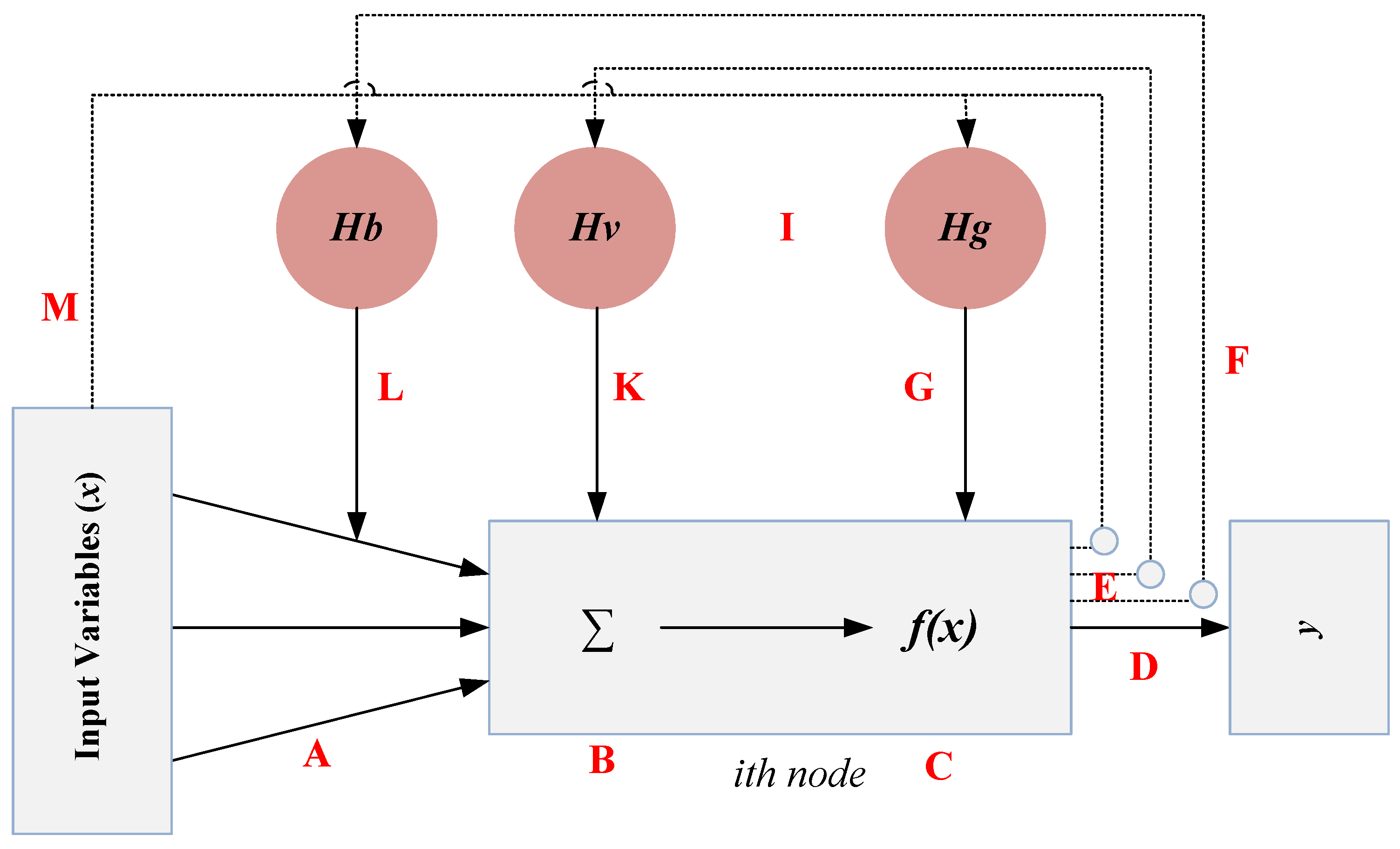
The ENN is a learning algorithm of backpropagation ANN; it is summarized in Biswas et al. [14]. Figure 1 proposed ENN diagram and processing. ENN includes an artificial emotion unit that used to improve the performance of network nodes, and the generated hormonal weights can be changed using the learning algorithm of the feedback loop (Figure 1) [29]. From Figure 1, the dynamic hormones of Hb, Hv, and Hg were given at each node. Hb, Hv, and Hg are produced and changed during the training phase and learning process, respectively. The hormonal coefficients, such as activation function, weights, and net function, can be determined and improved in the training stage. In Figure 1, the solid and dotted lines represent the neural and hormonal paths, respectively. Thus, the output (y) of the ith node of the ENN model with the three hormonal paths can be represented as [30]:

$$\begin{array}{c}{y}_i=\underset{1}{\underbrace{\left(w_i+{\displaystyle {\displaystyle \sum }_h}{\delta }_{i,h}{H}_h\right)}}\times f({\displaystyle {\displaystyle \sum }_j}[\underset{2}{\underbrace{\left({\beta }_i+{\displaystyle {\displaystyle \sum }_h}{\epsilon }_{i,h}{H}_h\right)}}\times \underset{3}{\underbrace{\left({\gamma }_{i,j}+{\displaystyle {\displaystyle \sum }_h}{\phi }_{i,j,k}{H}_h\right)}}{x}_{i,j}\\ +\underset{4}{\underbrace{\left({\mu }_i+{\displaystyle {\displaystyle \sum }_h}{\tau }_{i,h}{H}_h\right)}})\end{array}$$

(9)

where,

$$H={\displaystyle \sum }_i{H}_{i,h}; h=\left(b,v,g\right)$$

(10)

In Equation (9), part (1) represents the imposed weight to the activation function (f). It includes constant neural weight of $w_i$ as well as the dynamic hormonal weight of ${\sum }_h{\delta }_{i,h}{H}_h$. Section (2) consists of applied weight to the summation (net) function, part (3) contains executed weight to the input variables ($x_{i,j}$), and term (4) shows the bias of the summation function, both neural and hormonal weights of ${\mu }_i$ and ${\sum }_h{\tau }_{i,h}{H}_h$, respectively, were comprised.

The effect of systems hormonal level (Hh) in each hormonal weight is adjusted through ${\delta }_{i,h}, {\epsilon }_{i,h}, {\phi }_{i,j,k}, and {\tau }_{i,h}$ parameters and in turn, the model output of ith neuron ($y_i$) gives hormonal feedback of $H_{i,h}$ to the system as:

$$H_{i,h}=glandit{y}_{i,h}\times y_i$$

(11)

where, the $glandity$ factor should be improved in the training stage of ENN. Herein, the anxiety factor is prepared based on the change of input data of each training sample. However, at the first stage, the confidence factor is applied to connect the anxiety factor and the network output. For that, to set the hormonal values of Hh, some schemes can be considered, e.g., average of input variables of learning sample [31,32]. Here, the learning process is utilized to update the hormonal values to achieve the estimated values. Consequently, anxiety and confidence coefficients ($glandity$ factor) are significant parameters in ENN model. In this study, both parameters were used throughout the generalization and learning process. These parameters were supposed lies between 0 and 1. Furthermore, the trial-and-error method was used to determine ENN structure, neurons and layers numbers, to estimate the optimum S and CS estimation value.

2.2.4. ANN-PSO Model

A hybrid ANN-PSO is integration technique in-between ANN and PSO for the architecture of the ANN [33]. The details of ANN, PSO and ANN-PSO can be found in [22,33,34]. Herein, the output neuron (y) of ANN can be expressed as follows [33]:

$$y=\max \left(0,{{\displaystyle \sum }}_i{w}_i{x}_i+b\right)$$

(12)

where, $w, x, and b$ are the weight, input neuron, and bias, respectively.

The mapping between ANN layers can be presented as follows [33]:

$$h_i=\max \left(0,M_i{h}_{i-1}+b_i\right) for 1\le i\le L, and h_0=x$$

(13)

$$y=\max \left(0,V{h}_L\right)$$

(14)

where, L is the layers numbers, matrices M and V, and vector b are the learned parameters of ANN.

In ANN-PSO, the learned parameters of ANN can be estimated using PSO to minimize the classic ANN algorithm errors. Here, the mean square error (MSE) was defined as a fitness cost function into estimating the ANN parameters. The best model was achieved based on a lower value of MSE. The PSO started with generating a random swarm of particles for each parameter of ANN. Next, the swarm was updated based on the position update of particles. The updated circulated up to obtain the optimum position of particles. The position update can be expressed as follows [33]:

$$v_i^{t+1}=w{v}_i^t+c_1{r}_1\left(p_{best,i}^t-X_i^t\right)+c_2{r}_2\left(g_{best,i}^t-X_i^t\right)$$

(15)

$$X_i^{t+1}=X_i^t+v_i^{t+1}$$

(16)

where, $X and v$ denote the position and velocity of the particle, respectively; $w$ is the inertia parameter; $c_1 and c_2$ represent the cognitive and social component parameters, respectively. $r_1 and r_2$ are randomly assumed in between 0 and 1. $p_{best,i}^t and g_{best,i}^t$ are the best positions of the particle at individual and global positions, respectively.

In this study, the PSO was used to estimate the best parameters of ANN, number of hidden layers and neurons in each layer. Based on our trails, the best architecture of the ANN was achieved with 3 layers and 20 neurons, respectively, for estimating S of SCC; whereas, for CS, the 3 layers with 10 neurons were found the best performance. The $w, c_1 and c_2$ were selected to be $\frac{1+rand}{2}$, 1.0, and 2.0, respectively.

2.2.5. Models Processing and Performance Evaluation

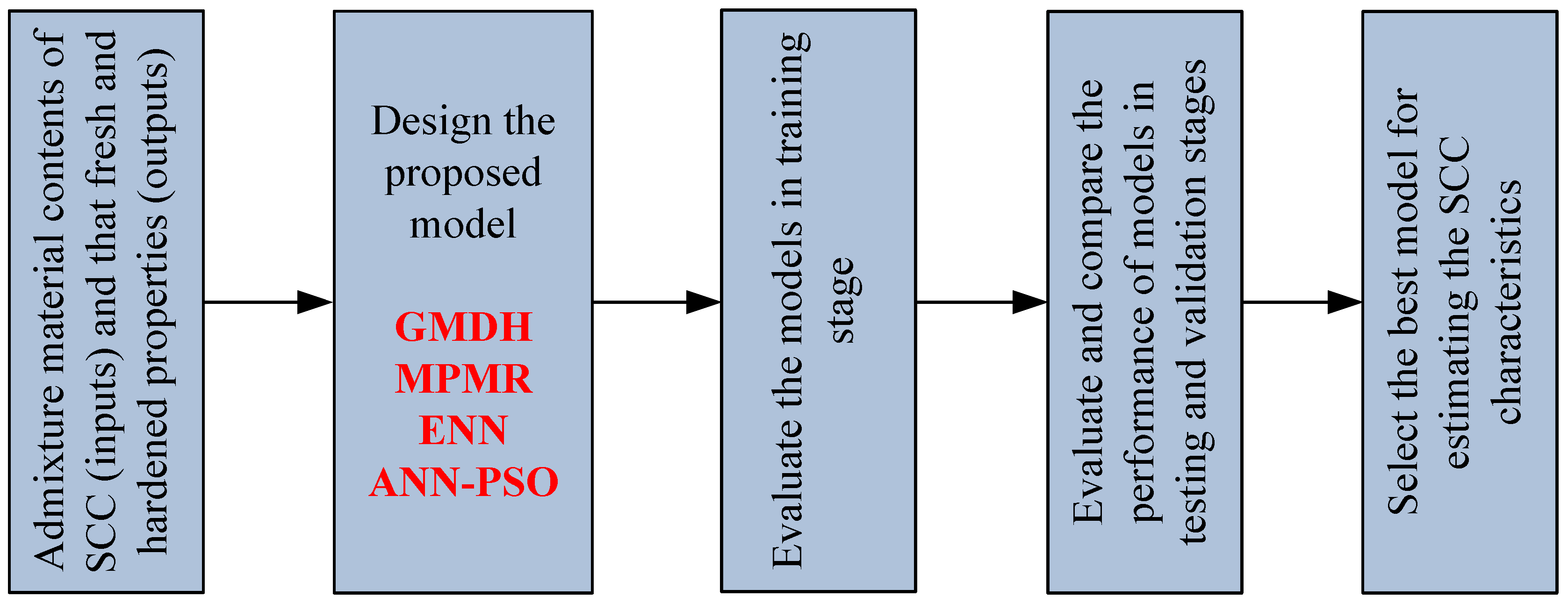
The processing steps of the proposed models were implemented through five stages as presented in Figure 2. MATLAB software was used to design and evaluate all models. Herein, eight variables are used as inputs for modeling S and CS of SCC. First, the whole data was normalized using Equation (17) for modeling, and output of models was inversed to original data for evaluation. Then, the data was divided into three categories, the training phase for designing the proposed models, testing phase for evaluating the models, and validation phase for qualify the models. The data was divided into 70% and 30% for the training and testing stages, respectively; whereas, the whole data was used in the validation phase. After that, the models were designed and evaluated in the training stage and compared in the testing stage. The models were evaluated and compared using a large number of data in the validation stage. Here, four statistical criteria, Equations (18)–(21), were applied to assess the performance of the proposed models; these are r (Equation (18)), RMSE (Equation (19)), mean absolute error (MAE) (Equation (20)), and percentage of RMSE (PE) (Equation (21)).

$$d_n=\left(D-D_{min}\right)/\left(D_{max}-D_{min}\right)$$

(17)

where, $d_n$ is the normalized data; D, D_max, and D_min are the data value, maximum and minimum data used, respectively.

$$r=\frac{{{\displaystyle \sum }}_{i=1}^N\left(S_o-S_{\overline{o}}\right)\left(S_p-S_{\overline{p}}\right)}{\sqrt{{{\displaystyle \sum }}_{i=1}^N{\left(S_o-S_{\overline{o}}\right)}^2{{\displaystyle \sum }}_{i=1}^N{\left(S_p-S_{\overline{p}}\right)}^2}}\times 100$$

(18)

$$RMSE=\sqrt{\frac{{{\displaystyle \sum }}_{i=1}^N{\left(S_p-S_o\right)}^2}{N}}$$

(19)

$$MAE=\frac{1}{N}{\displaystyle \sum }_{i=1}^N\left|S_p-S_o\right|$$

(20)

$$PE=\frac{RMSE}{S_{o\_mx}-S_{o\_mi}}\times 100$$

(21)

where $S_p and S_o$ are the estimated and measured values of S or CS, respectively; N is the number of samples; $S_{\overline{o}} and S_{\overline{p}}$ are the mean values of the estimated and measured values of S or CS, respectively, and $S_{o\_mx} and S_{o\_mi}$ are maximum and minimum values of measured S or CS, respectively.

2.3. Sensitivity Analysis

From the previous step, the optimum model for estimating S and CS of SCC can be obtained. The sensitivity of the eight variables was then investigated and studied in the optimal model. The inputs impact on the concrete slump and compressive strength was assessed by calculating a sensitivity index, which can be used to prove the significant input variables in the model. The sensitivity index would decrease in the admixture contents, which leads to a cost reduction of SCC. In the current study, a step-by-step method was implemented to detect the sensitivity of variables by varying each of the input variables at a constant rate. The sensitivity (Sv) of each variable was calculated as follows [11,35]:

$$Sv(\%) \mathrm{for} \mathrm{each} \mathrm{variable} =\left(\frac{1}{N}\right){{\displaystyle \sum }}_{j=1}^N{\left(\frac{\left(\%change in output\right)}{\left(\%change in input\right)}\right)}_j\times 100$$

(22)

where, N is the number of training data points. A constant rate of 20% was selected.

3. Results and Discussion

3.1. Slump Flow Modeling

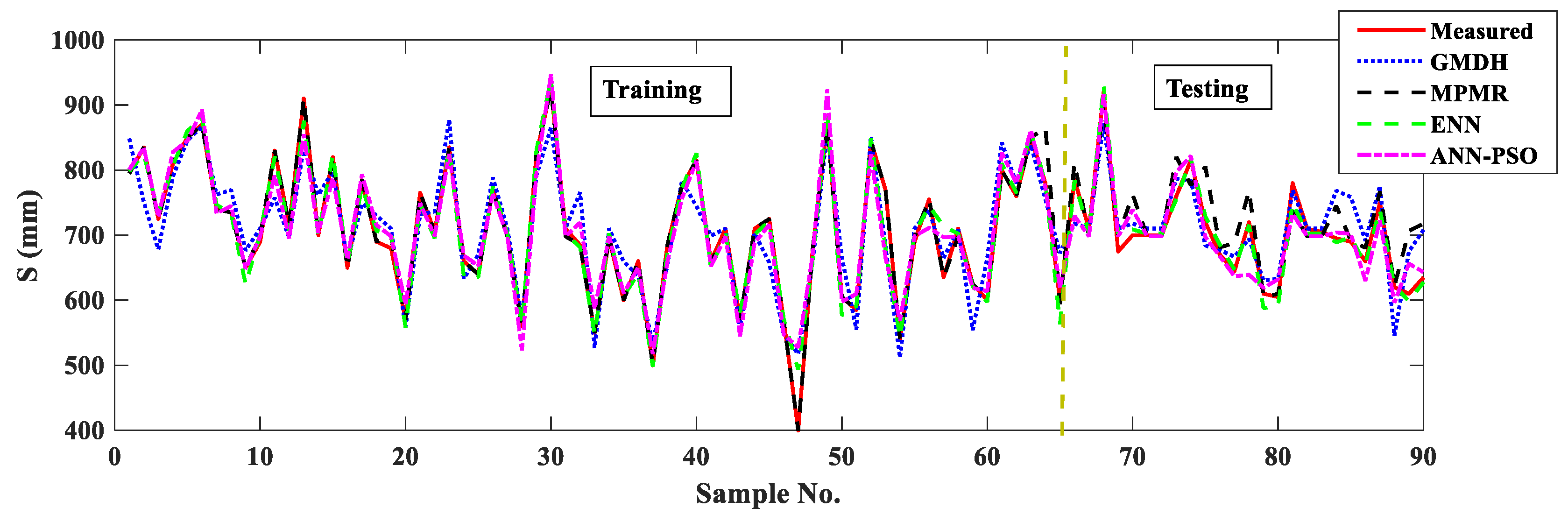
The performance of the proposed models for estimating S of SCC are presented in Figure 3 and Figure 4 and

Table 5. Performance assessment of the models for S estimation.

Statistical Parameter	GMDH	MPMR	ENN	ANN-PSO
	Training
RMSE (mm)	42.00	3.77	22.23	30.29
MAE (mm)	33.61	1.20	12.97	20.91
r (%)	91.63	99.94	97.73	95.76
PE (%)	8.00	0.72	4.23	5.77
	Testing
RMSE (mm)	41.75	43.34	13.26	28.67
MAE (mm)	33.87	31.89	9.53	21.52
r (%)	82.80	86.76	98.67	91.99
PE (%)	13.05	13.54	4.14	8.96
	Overall
RMSE (mm)	30.48	23.95	20.16	42.54
MAE (mm)	24.55	10.41	11.09	31.93
r (%)	94.89	97.15	97.80	90.17
PE (%)	5.81	4.56	3.84	8.10

. Figure 3 presents the measured slump flow and estimated values by the proposed models in the training and testing stages. Table 5 demonstrates the performance of models in the training, testing and validation stages. The scatterplot of the proposed models’ results compared by measured slump flow for the validation phase is presented in Figure 4. In the training stage, the performance of MPMR model is shown better than other models with RMSE = 3.77 mm and r = 99.94%. While the worst model for modeling S is the GMDH, with a percentage of model error is 8%. The performance of ENN and ANN-PSO models are shown acceptable, with a percentage of model’s errors are 4.23% and 5.77%, respectively. Meanwhile, the percentages of model’s errors in the testing stage are totally changed, with values of 4.14%, 8.96%, 13.05%, and 13.54% for the ENN, ANN-PSO, GMDH and MPMR models, respectively. The correlations between measured and estimated S are 98.67%, 91.99%, 86.76%, and 82.8% for the ENN, ANN-PSO, GMDH and MPMR models, respectively. These results indicate that the number of data affects the MPMR model performance. In addition, the performance of ENN model is the best with low numbers of data for the slump of SCC. Thus, the ENN model outperforms other models and can be used for modeling the slump behavior of SCC.

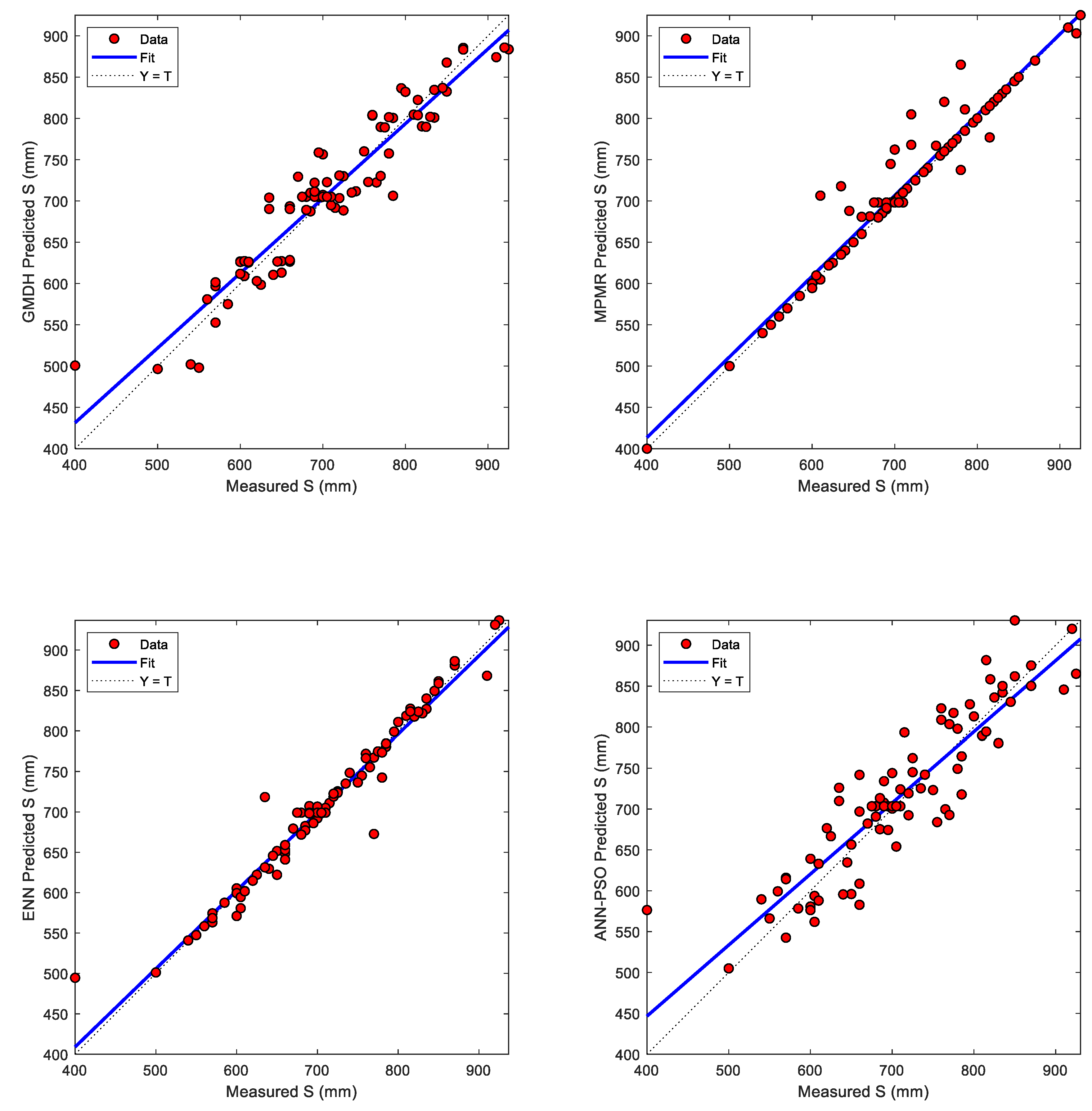
To validate the models’ performance, the entire data set was used to evaluate the quality of the models with a significant amount of data. From Table 5 and Figure 4, it can be shown that the robust model that can be used to estimate the slump flow of SCC is the ENN model. The percentage of the estimation error of the ENN model approached 3.8%. In addition, the closest model to the ENN model is the MPMR model; the performance of it is shown to be high with increasing the numbers of data.

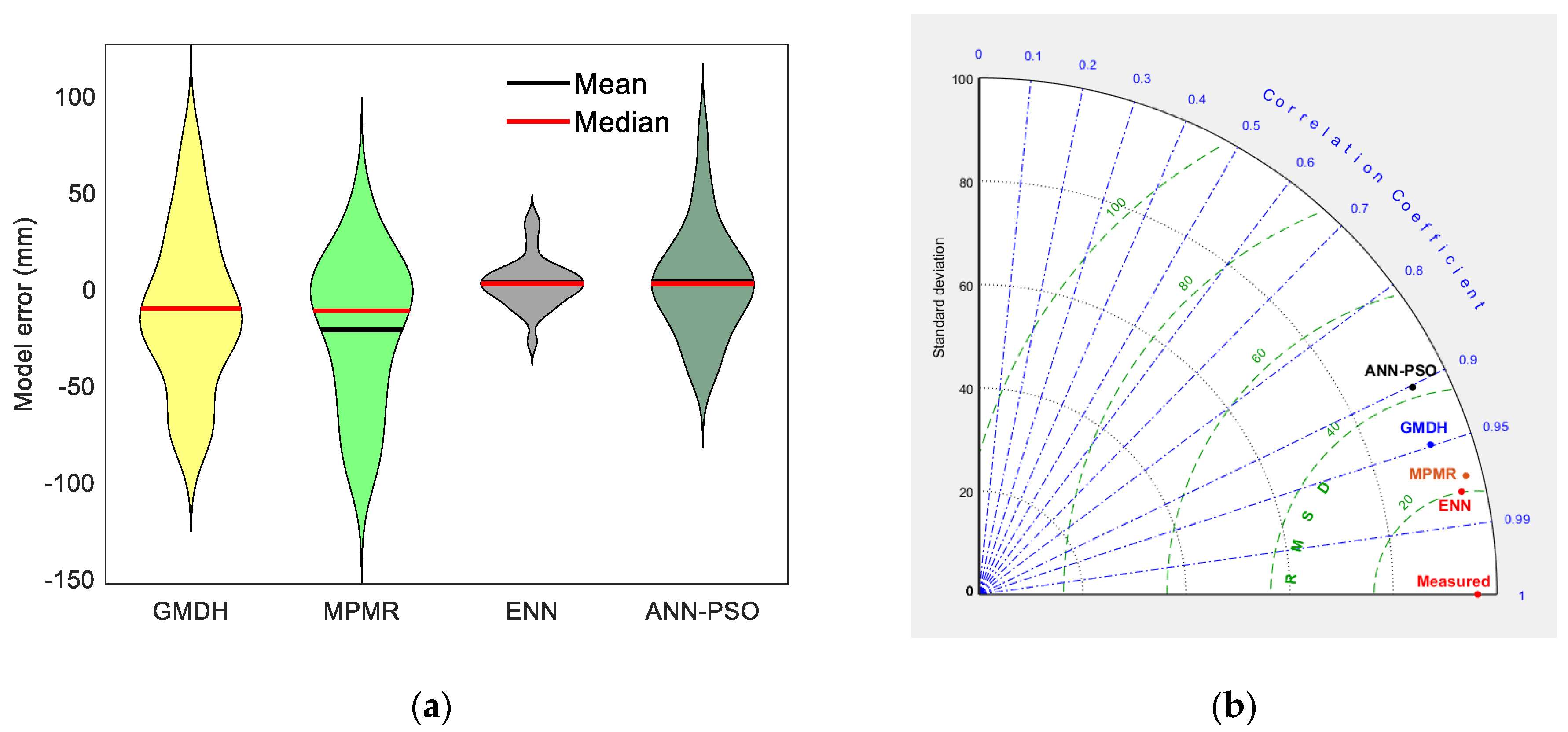
For further investigation into the performance of the proposed models with a low number of data (testing phase) and a large number of data (validation stage), the Violin and Taylor diagrams are presented in Figure 5a,b, respectively. The Violin plot was used to evaluate the model’s errors, and the estimated and measured data were assessed in the Taylor plot. It is obviously shown from Figure 5a that the ENN model is the best model that can be used to estimate the S of SCC. The distribution of errors is approximately normal with low outliers since the mean and median of model error is nearly same. Furthermore, summarize multiple statistical parameters were presented in Figure 5b for the models in the validation stage. The standard deviation, root mean square difference (RMSD) and r are presented in the diagram. From the figure, it can be clearly shown that the performance of ENN is better than other models for estimating the slump flow since it has a close performance model to the measured S values. From these results, it can be concluded that the ENN model can be used as a significant machine learning technique for estimating precise S values for the S data of SCC.

3.2. Compressive Strength Modeling

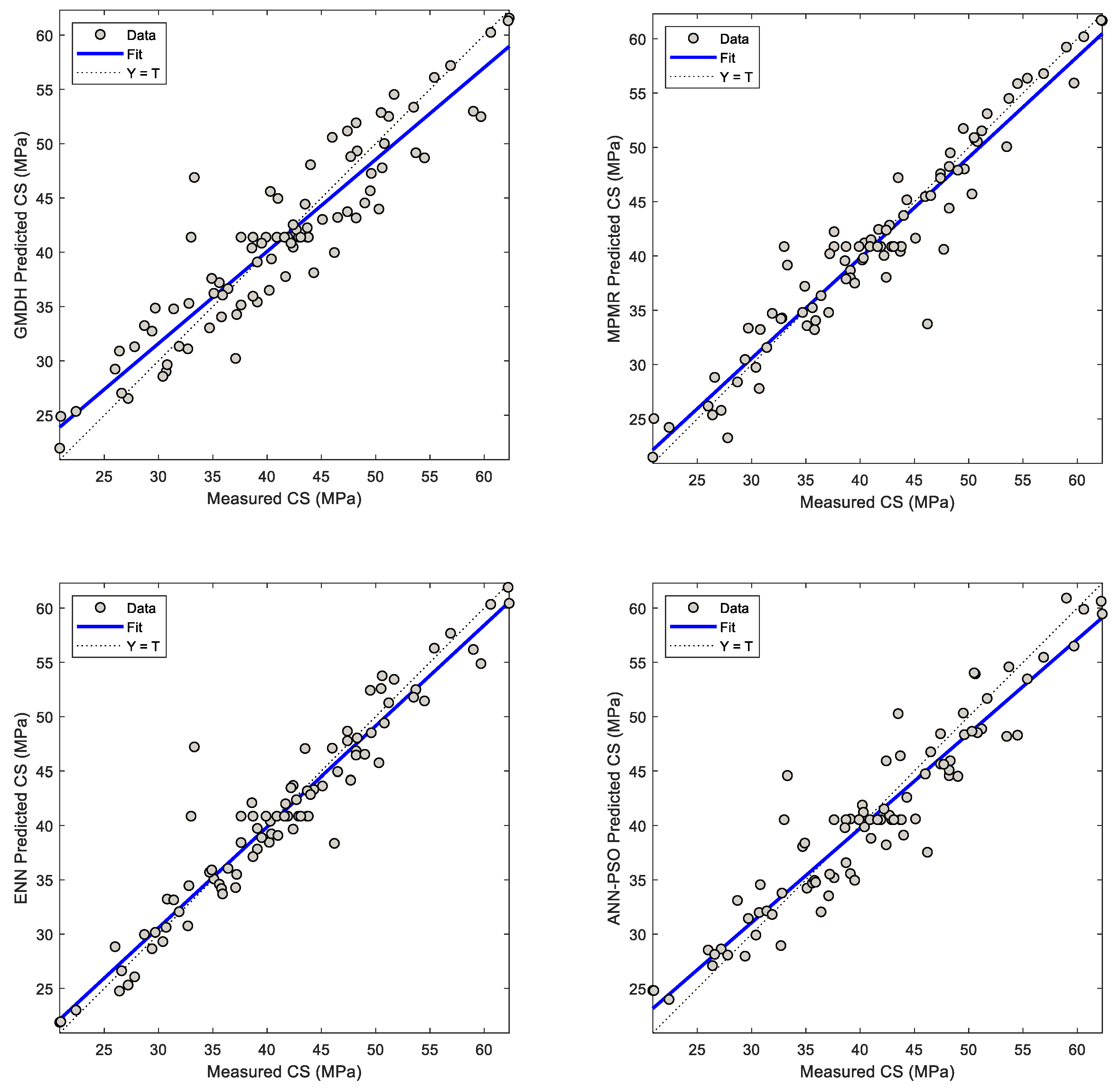
The four models with the eight input variables were used to estimate the compressive strength of SCC. The model’s performance in training and testing stage are compared in Figure 6. A high correlation between measured and estimated CS is observed with MPMR and ENN models in both stages. While maximum error can be observed with models GMDH and MPMR at training and testing stages, respectively.

Table 6. Performance assessment of the models for CS estimation.

Statistical Parameter	GMDH	MPMR	ENN	ANN-PSO
	Training
RMSE (MPa)	3.41	1.74	2.49	3.20
MAE (MPa)	2.62	1.25	1.64	2.12
r (%)	93.76	98.40	96.70	94.56
PE (%)	8.24	4.21	6.02	7.73
	Testing
RMSE (MPa)	3.65	4.08	2.78	2.88
MAE (MPa)	2.85	3.11	2.04	2.09
r (%)	89.79	86.97	94.36	93.54
PE (%)	10.62	11.86	8.08	8.37
	Overall
RMSE (MPa)	3.47	2.67	2.59	3.09
MAE (MPa)	2.66	1.81	1.77	2.43
r (%)	92.78	95.84	96.07	94.47
PE (%)	8.39	6.45	6.26	7.46

summarizes the performance of proposed models at training, testing and validation stages, and Figure 7 presents the performance of the four models in the validation stage.

The performance of MPMR model is also seen the best in the training stage, as presented in Table 6. The percentage error of the model is 4.21%; followed by the ENN model within 6.02% percentage error. In contrast, the best model in the testing and validation stages is ENN model within 8.08% and 6.26% percentage errors, respectively (see Table 6 and Figure 6 and Figure 7); while, the worst models’ performance in the testing and validation stages are the MPMR and GMDH models, respectively. Thus, the MPMR model is also influenced by the data number when used to estimate the CS of SCC. Here, the ENN model outperforms other models with RMSE = 2.59 MPa and r = 96.07% for the overall data. The MAE of ENN model for predicting CS of SCC is 1.77 MPa (a lower value compared by other models). These results reveal that the ENN model can be used as a soft computing model for detecting accurate CS of SCC with the eight inputs.

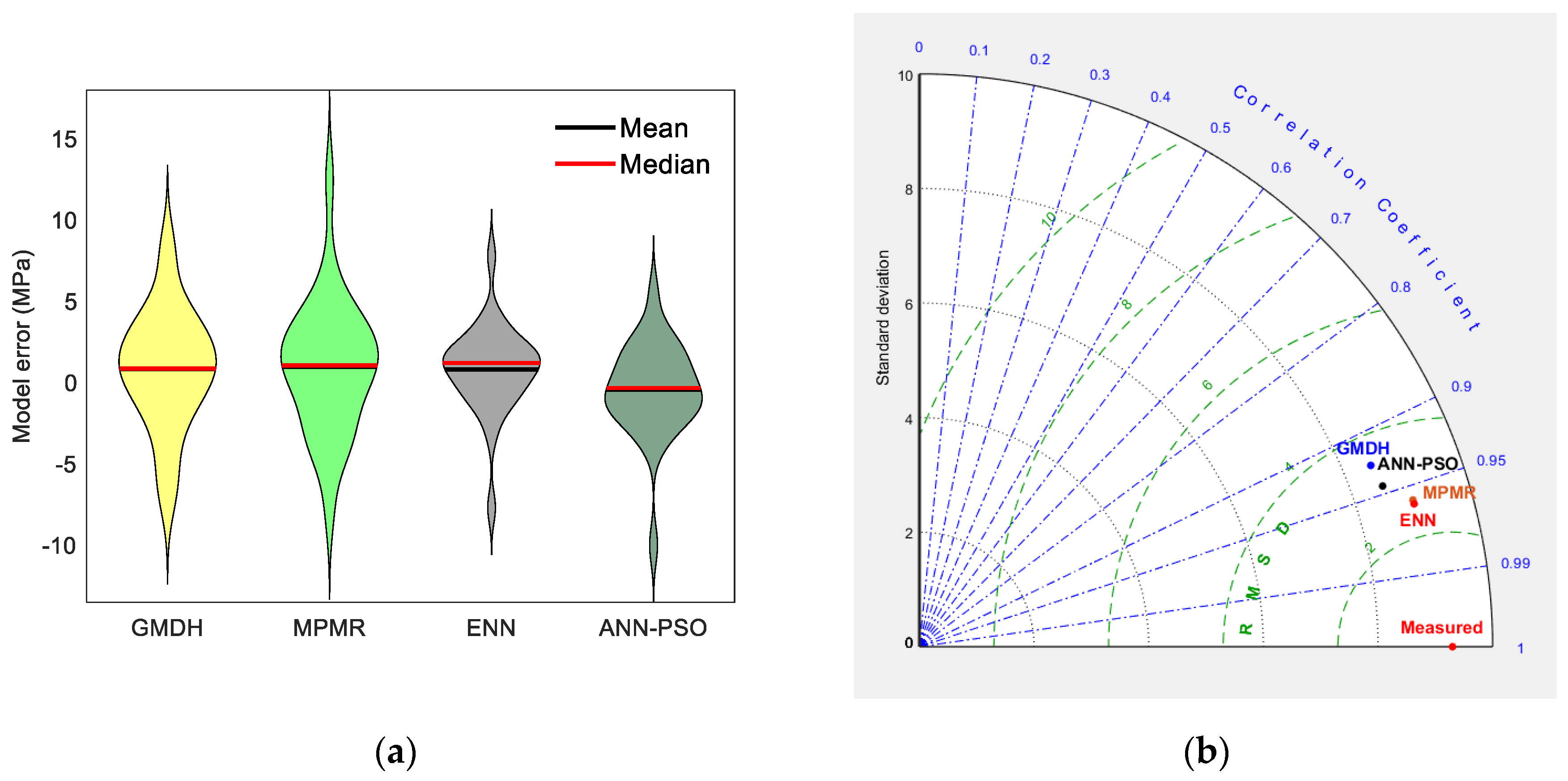
For more investigation, the performance of the proposed models in testing and validation phases were assessed. The Violin and Taylor diagrams for the testing and validation phases are presented in Figure 8a,b, respectively. The Violin plot for CS estimation also assessed the model’s errors, and the estimated and measured CS values were used in the Taylor plot. It is obviously shown from Figure 8a that the ENN model is the best model that can be used to estimate the CS of SCC. The distribution of errors is approximately normal with low outliers compared by other models, the average of maximum variation of model’s errors are about ±12.88 MPa, ±15.49 MPa, ±10.62 MPa, ±11.27 MPa. Some shift changes can be observed in the quartiles of Violin plot of ENN model, but it is still the best distribution among the four models.

In addition, a summary of multiple statistical parameters was presented in Figure 8b for the proposed models in the validation stage. From the figure, it can be clearly shown that the performance of ENN is better than other models for estimating the compressive strength of SCC since it possesses the close performance model to the measured CS values. Here, the performance of model MPMR is shown closer to the performance of the ENN model; but the data numbers still influence it (see Table 6 and Figure 6 and Figure 8a). From these results, it can also be concluded that the ENN model can be applied as a significant machine learning technique for estimating accurate CS values for the CS data of SCC.

3.3. The Sensitivity of Input Variables

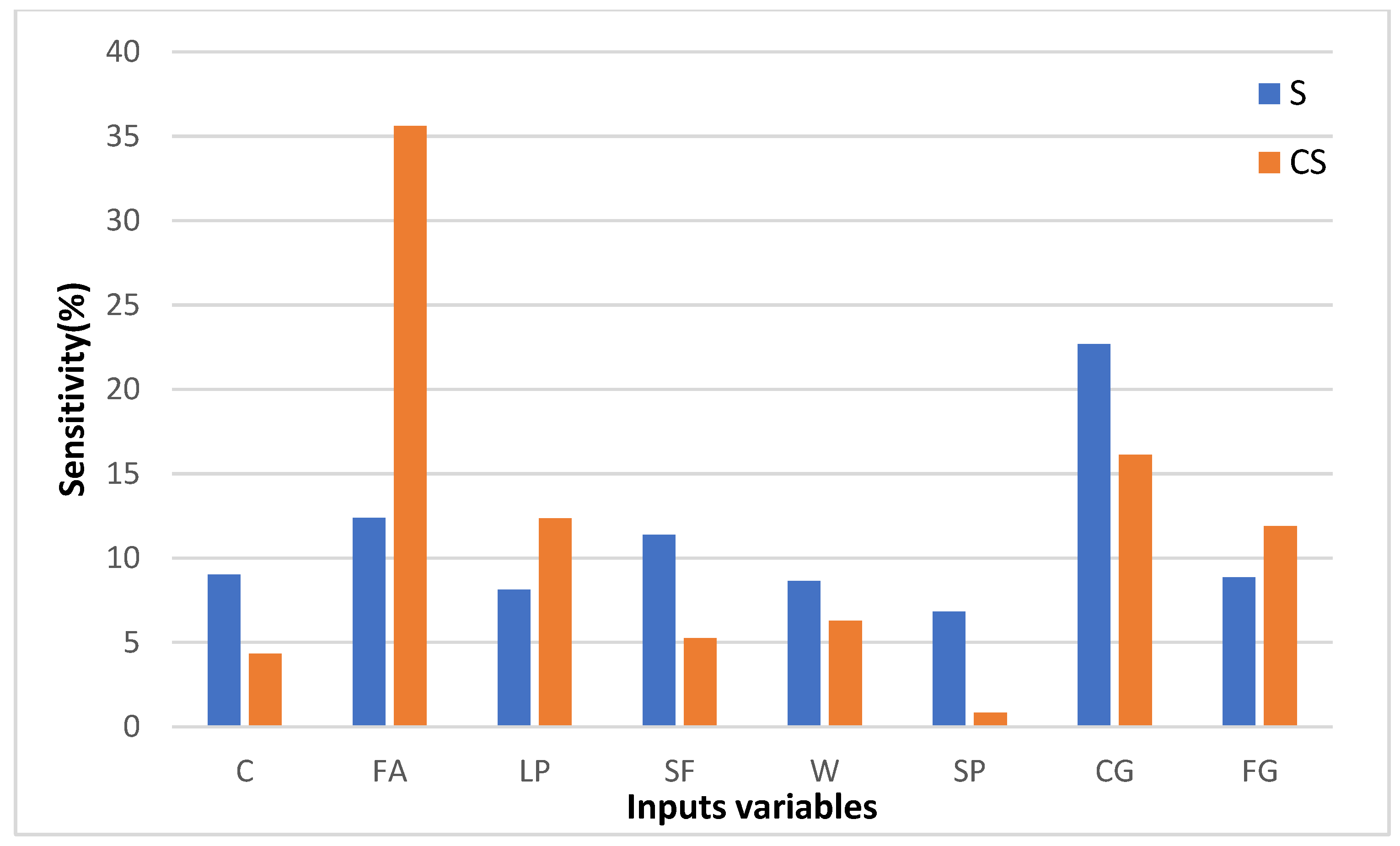
The input and output variables of the ENN models are used in Equation (22) to detect the impact of admixture contents on SCC characteristics. The calculated sensitivity of each variable in S and CS is presented in Figure 9. From the figure, it can be shown that the main components of the admixture affected SCC characteristics. The S and CS are influenced by the contents of the coarse and fine aggregate; while the FG percentage higher affected CS, the S is affected by the contents of CG. The effect of water content is shown to be high on S values compared to the effect on the CS values of SCC. Here, the SP effect is shown to be low on the CS properties of SCC. Meanwhile, the effect of powdered contents is shown to be high and has a different impact on S and CS values of SCC. The total effect of powdered materials on CS and S is 57.54% and 40.87%, respectively. Thus, the impact of total powdered content is high on the admixture content of SCC compared by other admixture materials. The minimal effect on S and CS from the whole admixture content is the SP percentage. When comparing the powder content, it can be seen that the FA affects the CS of SCC by 35.6%, followed by LP, SF, and C, respectively by 12.36%, 5.34%, 4.34%. While the impact of FA, LP, SF, and C on S of SCC is 12.37%, 8.11%, 11.38%, 9.01%, respectively. These results indicate that the FA can be considered as the main factor that affects the S and CS values of SCC, and the cement has a lower impact.

Thus, it can be concluded that the sensitivity of powder content of fly ash has a significant impact on the estimated S and CS values of SCC that contains FA, SF, and LP based on its mix design i.e., C, FA, SF, LP, W, SP, CG, FG. Herein, these results are shown coinciding with Elemam et al. [4], who concluded that the fresh and hardened characteristics of SCC are affected by the FA percentage. Aiyer et al. [36] also shown that the FA is the high impact factor for estimating CS of SCC containing C, FA, W, SP, CG, and FG. FA is also seen improved the mechanical performance of SCC that includes C, marble cutting slurry waste, FA, SF, W, SP, FG, and CG [37].

4. Conclusions

This study investigates to develop a novel machine learning method can be used to estimate the fresh and hardened characteristics of SCC. Four models, including GMDH, MPMR, ENN and hybrid ANN-PSO algorithms, are evaluated and compared to detect the slump flow and 28-day compressive strength of SCC. Laboratory data obtained from Elemam et al. [4] was used in this study. The data comprises FA, SF, and LP as part of the cement by mass in the total powder content. In addition, the impact of admixture contents is investigated for studying the effect of powder content of admixture, which would decrease the admixture cost of the SCC. Results of the model’s performance demonstrated that the developed ENN model was significantly trained, tested and validated for estimating the slump flow and compressive strength of SCC. In addition, it can be used as a machine learning technique for estimating the accurate slump flow and compressive strength values of SCC. The performance of MPMR was successfully trained to estimate the slump flow and compressive strength of SCC, but its performance with a low amount of an available data of SCC is shown to be lower than other models. The sensitivity analysis of input variables for estimating slump flow and compressive strength of SCC through ENN model shows that the impact of fly ash for detecting slump flow and compressive strength is 12.37% and 35.6%, respectively. Thus, the sensitivity of the powder content of fly ash is has a significant impact on the estimated SCC characteristics.

References

- Ghazanfari, N.; Gholami, S.; Emad, A.; Shekarchi, M. Evaluation of GMDH and MLP Networks for Prediction of Compressive Strength and Workability of Concrete. Bull. de la Société R. des Sci. Liège 2017, 86, 855–868. [Google Scholar]
- Sonebi, M.; Grünewald, S.; Cevik, A.; Walraven, J. Modelling fresh properties of self-compacting concrete using neural network technique. Comput. Concr. 2016, 18, 903–921. [Google Scholar] [CrossRef] [Green Version]
- Sobhani, J.; Najimi, M.; Pourkhorshidi, A.R.; Parhizkar, T. Prediction of the compressive strength of no-slump concrete: A comparative study of regression, neural network and ANFIS models. Constr. Build. Mater. 2010, 24, 709–718. [Google Scholar] [CrossRef]
- Elemam, W.E.; Abdelraheem, A.H.; Mahdy, M.G.; Tahwia, A.M. Optimizing fresh properties and compressive strength of self-consolidating concrete. Constr. Build. Mater. 2020, 249, 118781. [Google Scholar] [CrossRef]
- Gholhaki, M.; Kheyroddin, A.; Hajforoush, M.; Kazemi, M. An investigation on the fresh and hardened properties of self-compacting concrete incorporating magnetic water with various pozzolanic materials. Constr. Build. Mater. 2018, 158, 173–180. [Google Scholar] [CrossRef]
- Timur Cihan, M. Prediction of Concrete Compressive Strength and Slump by Machine Learning Methods. Adv. Civ. Eng. 2019, 2019, 1–11. [Google Scholar] [CrossRef]
- Öztaş, A.; Pala, M.; Özbay, E.; Kanca, E.; Çaǧlar, N.; Bhatti, M.A. Predicting the compressive strength and slump of high strength concrete using neural network. Constr. Build. Mater. 2006, 20, 769–775. [Google Scholar] [CrossRef]
- Jalal, M.; Mansouri, E.; Sharifipour, M.; Pouladkhan, A.R. Mechanical, rheological, durability and microstructural properties of high performance self-compacting concrete containing SiO2 micro and nanoparticles. Mater. Des. 2012, 34, 389–400. [Google Scholar] [CrossRef]
- Sabet, F.A.; Libre, N.A.; Shekarchi, M. Mechanical and durability properties of self consolidating high performance concrete incorporating natural zeolite, silica fume and fly ash. Constr. Build. Mater. 2013, 44, 175–184. [Google Scholar] [CrossRef]
- Leung, H.Y.; Kim, J.; Nadeem, A.; Jaganathan, J.; Anwar, M.P. Sorptivity of self-compacting concrete containing fly ash and silica fume. Constr. Build. Mater. 2016, 113, 369–375. [Google Scholar] [CrossRef] [Green Version]
- Dutta, S.; Samui, P.; Kim, D. Comparison of machine learning techniques to predict compressive strength of concrete. Comput. Concr. 2018, 21, 463–470. [Google Scholar]
- Belalia Douma, O.; Boukhatem, B.; Ghrici, M.; Tagnit-Hamou, A. Prediction of properties of self-compacting concrete containing fly ash using artificial neural network. Neural Comput. Appl. 2017, 28, 707–718. [Google Scholar] [CrossRef]
- Ding, Z.; An, X. Deep Learning Approach for Estimating Workability of Self-Compacting Concrete from Mixing Image Sequences. Adv. Mater. Sci. Eng. 2018, 2018, 6387930. [Google Scholar] [CrossRef] [Green Version]
- Biswas, R.; Samui, P.; Rai, B. Determination of compressive strength using relevance vector machine and emotional neural network. Asian J. Civ. Eng. 2019, 20, 1109–1118. [Google Scholar] [CrossRef]
- Madandoust, R.; Bungey, J.H.; Ghavidel, R. Prediction of the concrete compressive strength by means of core testing using GMDH-type neural network and ANFIS models. Comput. Mater. Sci. 2012, 51, 261–272. [Google Scholar] [CrossRef]
- Madandoust, R.; Ghavidel, R.; Nariman-Zadeh, N. Evolutionary design of generalized GMDH-type neural network for prediction of concrete compressive strength using UPV. Comput. Mater. Sci. 2010, 49, 556–567. [Google Scholar] [CrossRef]
- Jang, Y.; Ahn, Y.; Kim, H.Y. Estimating Compressive Strength of Concrete Using Deep Convolutional Neural Networks with Digital Microscope Images. J. Comput. Civ. Eng. 2019, 33, 1–11. [Google Scholar] [CrossRef]
- Nikoo, M.; Torabian Moghadam, F.; Sadowski, Ł. Prediction of concrete compressive strength by evolutionary artificial neural networks. Adv. Mater. Sci. Eng. 2015, 2015, 849126. [Google Scholar] [CrossRef]
- Safiuddin, M.; Raman, S.N.; Salam, M.A.; Jumaat, M.Z. Modeling of compressive strength for self-consolidating high-strength concrete incorporating palm oil fuel ash. Materials 2016, 9, 396. [Google Scholar] [CrossRef]
- Yang, D.-S.; Park, S.-K.; Lee, J.-H. A prediction on mix proportion factor and strength of concrete using neural network. KSCE J. Civ. Eng. 2003, 7, 525–536. [Google Scholar] [CrossRef]
- Sadowski, Ł.; Nikoo, M.; Nikoo, M. Concrete compressive strength prediction using the imperialist competitive algorithm. Comput. Concr. 2018, 22, 355–363. [Google Scholar]
- Shariati, M.; Mafipour, M.S.; Mehrabi, P.; Bahadori, A.; Zandi, Y.; Salih, M.N.A.; Nguyen, H.; Dou, J.; Song, X.; Poi-Ngian, S. Application of a hybrid artificial neural network-particle swarm optimization (ANN-PSO) model in behavior prediction of channel shear connectors embedded in normal and high-strength concrete. Appl. Sci. 2019, 9, 5534. [Google Scholar] [CrossRef] [Green Version]
- Tien Bui, D.; Abdullahi, M.M.; Ghareh, S.; Moayedi, H.; Nguyen, H. Fine-tuning of neural computing using whale optimization algorithm for predicting compressive strength of concrete. Eng. Comput. 2019, in press. [Google Scholar] [CrossRef]
- Golafshani, E.M.; Pazouki, G. Predicting the compressive strength of self-compacting concrete containing fly ash using a hybrid artificial intelligence method. Comput. Concr. 2018, 22, 419–437. [Google Scholar]
- Koopialipoor, M.; Nikouei, S.S.; Marto, A.; Fahimifar, A.; Jahed Armaghani, D.; Mohamad, E.T. Predicting tunnel boring machine performance through a new model based on the group method of data handling. Bull. Eng. Geol. Environ. 2019, 78, 3799–3813. [Google Scholar] [CrossRef]
- Strohmann, T.; Grudic, G.Z. A formulation for minimax probability machine regression. Adv. Neural Inf. Proc. Syst. 2003, 15, 785–792. [Google Scholar]
- Kumar, M.; Mittal, M.; Samui, P. Performance assessment of genetic programming (GP) and minimax probability machine regression (MPMR) for prediction of seismic ultrasonic attenuation. Earthq. Sci. 2013, 26, 147–150. [Google Scholar] [CrossRef] [Green Version]
- Samui, P.; Kim, D.; Jagan, J.; Roy, S.S. Determination of Uplift Capacity of Suction Caisson Using Gaussian Process Regression, Minimax Probability Machine Regression and Extreme Learning Machine. Iran. J. Sci. Technol. Trans. Civ. Eng. 2019, 43, 651–657. [Google Scholar] [CrossRef]
- Sharghi, E.; Nourani, V.; Molajou, A.; Najafi, H. Conjunction of emotional ANN (EANN) and wavelet transform for rainfall-runoff modeling. J. Hydroinformatics 2019, 21, 136–152. [Google Scholar] [CrossRef] [Green Version]
- Nourani, V. An Emotional ANN (EANN) approach to modeling rainfall-runoff process. J. Hydrol. 2017, 544, 267–277. [Google Scholar] [CrossRef]
- Kumar, S.; Roshni, T.; Himayoun, D. A Comparison of Emotional Neural Network (ENN) and Artificial Neural Network (ANN) Approach for Rainfall-Runoff Modelling. Civ. Eng. J. 2019, 5, 2120–2130. [Google Scholar] [CrossRef]
- Lotfi, E.; Akbarzadeh, M. Practical emotional neural networks. Neural Netw. 2014, 59, 61–72. [Google Scholar] [CrossRef] [PubMed]
- Qi, C.; Fourie, A.; Chen, Q. Neural network and particle swarm optimization for predicting the unconfined compressive strength of cemented paste backfill. Constr. Build. Mater. 2018, 159, 473–478. [Google Scholar] [CrossRef]
- Kaloop, M.R.; Kumar, D.; Samui, P.; Gabr, A.R.; Hu, J.W.; Jin, X.; Roy, B. Particle Swarm Optimization algorithm-Extreme Learning Machine (PSO-ELM) model for predicting resilient modulus of stabilized aggregate bases. Appl. Sci. 2019, 9, 3221. [Google Scholar] [CrossRef] [Green Version]
- Liong, S.-Y.; Lim, W.-H.; Paudyal, G. River stage forecasting in Bangladish: Neural network approach. J. Comput. Civ. Eng. 2000, 14, 1–8. [Google Scholar] [CrossRef]
- Aiyer, B.G.; Kim, D.; Karingattikkal, N.; Samui, P.; Rao, P.R. Prediction of compressive strength of self-compacting concrete using least square support vector machine and relevance vector machine. KSCE J. Civ. Eng. 2014, 18, 1753–1758. [Google Scholar] [CrossRef]
- Choudhary, R.; Gupta, R.; Nagar, R. Impact on fresh, mechanical, and microstructural properties of high strength self-compacting concrete by marble cutting slurry waste, fly ash, and silica fume. Constr. Build. Mater. 2020, 239, 117888. [Google Scholar] [CrossRef]
Figure 1.
The emotional neural network (ENN) structure network (A, B, and C are the weights to input, net and activation functions, respectively; E is glandity; I represents the hormonal unit; D, M, F, G, K, and L are weights applied on net output, hormones from input/output, activation function, net function, and input static weights, respectively).
Figure 2.
Flowchart of models processing and evaluation.
Figure 3.
The performance of the models compared by slump measured values in the training and testing stages.
Figure 4.
Scatterplot of proposed models with measured slump flow in the validation stage.
Figure 5.
Performance of models for slump modeling based on the number of data. (a) Violin diagram for the testing stage; (b) Taylor diagram for the validation stage.
Figure 6.
The performance of the models compared by compressive strength measured values in the training and testing stages.
Figure 7.
Scatterplot of proposed models with measured compressive strength in the validation stage.
Figure 8.
Performance of models for compressive strength modeling based on the number of data. (a) Violin diagram for the testing stage; (b) Taylor diagram for the validation stage.
Figure 9.
Sensitivity index of input variables for estimating S and CS of SCC.