Machine Learning Approaches for Detecting Parkinson’s Disease from EEG Analysis: A Systematic Review

Abstract

Background: Diagnosis of Parkinson’s disease (PD) is mainly based on motor symptoms and can be supported by imaging techniques such as the single photon emission computed tomography (SPECT) or M-iodobenzyl-guanidine cardiac scintiscan (MIBG), which are expensive and not always available. In this review, we analyzed studies that used machine learning (ML) techniques to diagnose PD through resting state or motor activation electroencephalography (EEG) tests. Methods: The review process was performed following Preferred Reporting Items for Systematic Reviews and Meta-Analyses (PRISMA) guidelines. All publications previous to May 2020 were included, and their main characteristics and results were assessed and documented. Results: Nine studies were included. Seven used resting state EEG and two motor activation EEG. Subsymbolic models were used in 83.3% of studies. The accuracy for PD classification was 62–99.62%. There was no standard cleaning protocol for the EEG and a great heterogeneity in the characteristics that were extracted from the EEG. However, spectral characteristics predominated. Conclusions: Both the features introduced into the model and its architecture were essential for a good performance in predicting the classification. On the contrary, the cleaning protocol of the EEG, is highly heterogeneous among the different studies and did not influence the results. The use of ML techniques in EEG for neurodegenerative disorders classification is a recent and growing field.

1. Introduction

Parkinson’s disease (PD) is the second most common neurological disease after Alzheimer’s disease, affecting 2–3% of the population older than 65 years of age [1]. It is characterized by the loss of dopaminergic neurons in the substantia nigra [2]. The diagnosis of PD relies on the presence of motor symptoms (bradykinesia, rigidity and tremor at rest [3]). However, autopsy and neuroimaging studies indicate that the motor signs of PD are a late manifestation that is evident when the degree of degeneration of dopaminergic neurons is 50–70% [4,5].

There are a wide variety of techniques in the field of neurology that are used individually or in combination to support the clinical diagnosis. Commonly used techniques include image-based tests (single photon emission computed tomography (SPECT), M-iodobenzyl-guanidine cardiac scintiscan (MIBG)), however, these are costly and are not always accessible.

Electroencephalography (EEG) is a non-invasive technique that records the electrical activity of the pyramidal neurons of the brain, giving an indirect insight of their function with a great time resolution. It has been widely used to study epileptic disorders and is a widely accessible and low-cost technique. Visual EEG analysis is the gold standard for clinical EEG interpretation and analysis, but the information processing techniques allow for the extraction of different characteristics that can be of help when characterizing neurological diseases.

Due to its good temporal resolution, EEG data provide dynamic information on the electrical brain activity and connectivity. For this reason, EEG has been recorded in different physiological conditions such as basal awake condition, during sleep, during specific sensitive input or cognitive tasks and finally in resting state. During each of these conditions, different networks are expected to be activated and spontaneous connectivity is expected in resting state.

In addition to the well known inter/intra-subjects’ variability, two main characteristics define the EEG signals and make their subsequent analysis difficult. These are the low signal-to-noise ratio and the stochastic nature of the signals. A low signal-to-noise ratio indicates a high level of noise in EEG signals, so pre-processing is required to filter out the signal noise and to remove the possible artifacts, such as contamination by other biological and non-biological signal sources, and then analyze the signals and obtain results. The main problem to filter the signals is that there are several validated protocols with no gold standard defined to perform the cleaning. Another problem comes from the fact that when the signal noise is removed, relevant components in EEG signals can also be eliminated, which may lead to false diagnosis. On the other hand, the stochastic character indicates that the state or occurrence of an event does not depend on the previous event. Hence, to extract the essential characteristics of the signals, advanced non-linear techniques must be used, which require more expensive computational methods [6,7,8]. These difficulties can be overcome by implementing machine learning (ML) techniques to analyze the EEG signals, since they are quite strong techniques that allow to carry out studies of non-linear nature, as well as to deal with raw EEGs.

Machine learning is a discipline of artificial intelligence that develops algorithms with the capacity to generalize behaviors and recognize hidden patterns in a large amount of data, defined by Arthur Samuel as the “field of study that gives computers the ability to learn without being explicitly programmed” [9]. ML techniques can be classified into two categories depending on the type of processing that is carried out: symbolic processing, which uses formal languages, logical orders, and symbols, and subsymbolic processing, which is designed to estimate functional relationships between data. Within ML techniques, artificial neural networks (ANN) are those whose architecture is based in multiple-layer hierarchical models that can learn representations of data with multiple levels of abstraction. However, they require a large amount of input data and a careful training process. All these techniques are receiving increasing interest from the medical domain, where they have been mostly used in image analysis [10], although in recent years, their application has spread to other areas [11,12].

The analysis of EEG has already been used in other non-epileptic neurological diseases such as Alzheimer’s, schizophrenia, and major depressive disorder [13,14,15] and there are numerous articles that apply ML techniques to study their EEG [16,17,18,19,20,21,22,23]. EEG processing using ML techniques has also been used for therapeutical purposes such as stroke rehabilitation [24]. The use of EEG to study Parkinson’s disease has not been fully validated, but in the last 5 years, its interest has increased with the introduction of ML techniques in EEG analysis, leading to a growing development of the literature. The aim of this review consists, firstly, in evaluating the current impact of ML techniques on the EEG analysis of patients with PD, and secondly, naming the most commonly used techniques and analyzing those that have provided the best results. These objectives, focused on the diagnosis and evolution of PD, will provide an entry point for further studies seeking to determine an early, non-invasive and accessible diagnostic marker that minimizes the delay on the disease diagnosis. Hopefully, the advances in new diagnostic techniques in PD could help to detect this disease in its early stages, that is, in pre-motor stage, favoring the development of preventive therapies that slow the degree of advancement of motor and cognitive decline in PD [25].

2. Methods

2.1. PRISMA Statement

With the main objective of assuring the quality of this systematic review, the selection process followed the Preferred Reporting Items for Systematic Reviews and Meta-Analyses (PRISMA—http://www.prisma-statement.org) guidelines. For more information about the review protocols, see the Statement article [26] and the Explanation and Elaboration article [27].

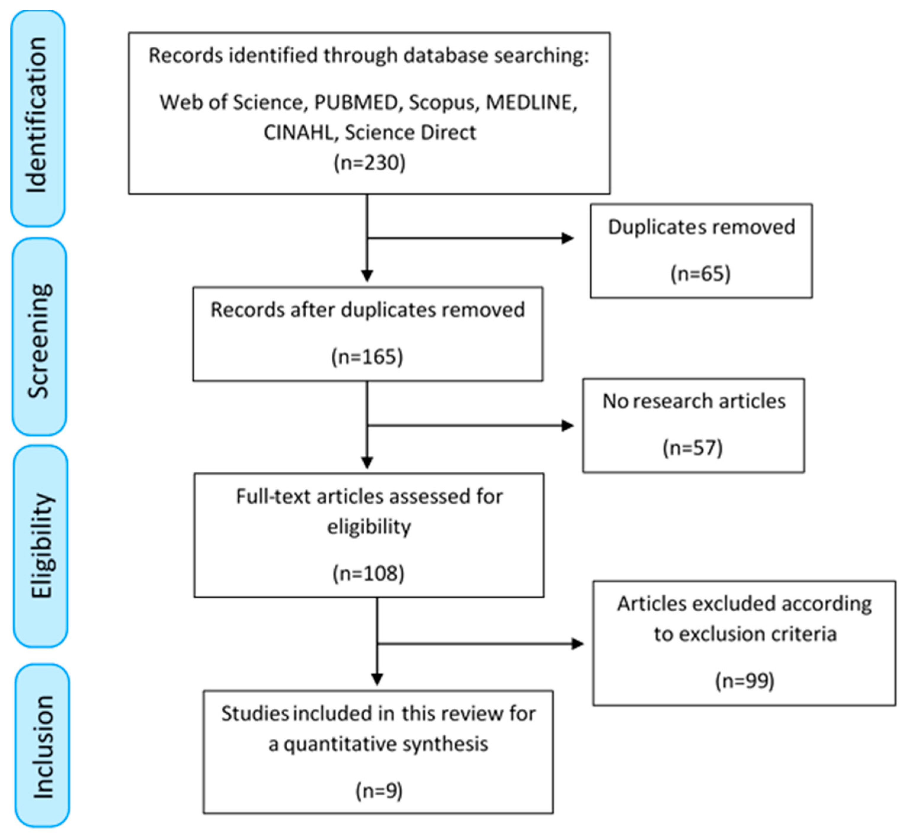
Figure 1 shows the PRISMA flow diagram, which summarizes the search, screening and eligibility processes carried out in this review. The precise information of each of the steps is detailed in the sections below.

2.2. Identification: Search Strategy and Sources

The following terms were selected: 1. Parkinson’s; 2. EEG; 3. electroencephalogram; 4. machine learning; 5. deep learning; and 6. neural networks. The proposed search terms were combined using logical operators as follows: 1 AND (4 OR 5 OR 6) AND (2 OR 3). This combination was introduced in the following 6 databases: Web of Science, PUBMED, Scopus, MEDLINE, CINAHL and Science Direct. The search was performed on 19 May 2020, with no time limit, providing a total of 230 results.

2.3. Screening and Eligibility

The screening process was carried out in two steps. First, duplicates were removed. Second, with the main aim of removing the studies that had not been peer reviewed, only those publications cataloged as research articles were considered, even if they were not indexed in the Journal Citation Reports (JCRs) of Clarivate Analytics (http://jcr.clarivate.com). Thus, proceedings, conference articles, chapters in books, posters and editorials were excluded.

Within the eligibility process, the inclusion and exclusion criteria were applied, according to the objective of this review. For this purpose, two review authors (J.P.R. and A.M.M.) screened the title, the abstract, and the full article, if necessary, to determine if they satisfied the selection criteria. Any disagreement was resolved through consensus. The search was limited to studies written in English and Spanish. Inclusion criteria were: prospective or retrospective studies using EEG to assess PD progression or diagnosis using different ML architectures in awake surface EEG recordings. The exclusion criteria were: studies that did not consider EEGs, studies that did not use ML techniques for EEG analysis, studies that focused their analysis on other neurological diseases, animal studies, pharmacological studies, articles studying evoked changes in EEGs due to exogenous stimuli, invasive and sleep EEG recordings. Finally, those studies that did not include information about the methodology were omitted. As a consequence, the resulting selected articles consisted of PD studies that sought to diagnose or determine the evolution of this disease, by means of using ML techniques in resting state EEG tests or motor activation EEG tests.

2.4. Data Extraction and Analysis

Once the inclusion and exclusion criteria were applied, two review authors independently screened the full-text articles to obtain a score in the checklist as proposed in the Guidelines for Developing and Reporting Machine Learning Predictive Models in Biomedical Research [28]. The checklist consists of 12 reporting items to be included in a research article in order to assure the good quality of the article. The categories evaluated through the checklist include requirements within the field of biomedicine, the field of computer science, and requirements on how these two fields overlap with each other. The precise descriptions of the checklist items displayed in

Table 1. Items to include when reporting predictive models in biomedical research. Luo et al., 2016 [28].

Item	Section	Topic	Checklist Item
1	Title	Nature of study	Identify the report as introducing a predictive model.
2	Abstract	Structured summary	Background. Objectives. Data sources. Performance metrics of the predictive models (in both point estimates and confidence intervals). Conclusion including the practical value of the developed predictive model or models.
3	Introduction	Rationale	Identify the clinical goal. Review the current practice and prediction accuracy of any existing models.
4		Objectives	State the nature of study being predictive modeling, defining the target of prediction. Identify how the prediction problem may benefit the clinical goal.
5	Methods	Describe the setting	Identify the clinical setting for the target predictive model. Identify the modeling context in terms of facility type, size, volume, and duration of available data.
6		Define the prediction problem	Define a measure for the prediction goal. Identify the problem to be prognostic or diagnostic. Determine the form of the prediction model: classification, regression, or survival prediction. Explain practical costs of prediction errors. Define quality metrics for prediction models. Define the success criteria for prediction.
7		Prepare data for model building	Identify relevant data sources and quote the ethics approval number for data access. State the inclusion and exclusion criteria for data. Describe the time span of data and the sample or cohort size. Define the observational units on which the response variable and predictor variables are defined. Define the predictor variables. Describe the data pre-processing performed, including data cleaning and transformation. State any criteria used for outlier removal. State how missing values were handled. Describe the basic statistics of the dataset as the ratio of positive to negative classes for a classification problem. Define the model validation strategies. Define the validation metrics. For classification problems, the metrics should include sensitivity, specificity, positive predictive value, negative predictive value, area under the ROC curve, and calibration plot.
8		Build the predictive model	Identify independent variables that predominantly take a single value. Identify and remove redundant independent variables. Identify the independent variables that may suffer from the perfect separation problem. Assess whether sufficient data are available for a good fit of the model. Determine a set of candidate modeling techniques. If only one type of model was used, justify the decision for using that model. Define the performance metrics to select the best model.
9	Results	Report the final model and performance	Report the predictive performance of the final model in terms of the validation metrics specified in the methods section. If possible, report the parameter estimates in the model and their confidence intervals. When the direct calculation of confidence intervals is not possible, report nonparametric estimates from bootstrap samples. Comparison with other models in the literature should be based on confidence intervals. Interpretation of the final model. If possible, report what variables were shown to be predictive of the response variable. State which subpopulation has the best prediction and which subpopulation is most difficult to predict.
10	Discussion	Clinical implications	Report the clinical implications derived from the obtained predictive performance.
11		Limitations of the model	Discuss the following potential limitations: assumed input and output data format. Potential pitfalls in interpreting the model. Potential bias of the data used in modeling. Generalizability of the data.
12		Unexpected results during the experiments	Report unexpected signs of coefficients, indicating collinearity or complex interaction between predictor variables.

are summarized in the following points, which were the ones mainly considered for the assessment:

• Items 1, 2: the structure and content of the title and abstract are evaluated;
• Items 3, 4: the clinical objective is identified, the state of the art of existing models is reviewed and the study is justified;
• Items 5, 6: the dataset is described, providing an assessment of its quality and justifying the chosen model;
• Item 7: data pre-processing and validation metrics are described;
• Item 8: the model is described, providing sufficient information about the parameters that define its architecture for its reproducibility. It is evaluated whether the available data are sufficient for a good fit of the model;
• Item 9: the predictive performance of the model is provided in terms of the validation metrics;
• Items 10, 11, 12: the clinical implications of the results obtained are provided, limitations of the study are discussed, and unexpected results are reported.

The evaluation of each article through the checklist of Table 1 carried out by 2 independent evaluators (A.M. and P.C.) minimized the bias produced by a single reviewer. To measure the consensus between both evaluations taking into account the option of agreement by chance, the kappa value between both evaluations was calculated (>0.7 means a high level of agreement among the evaluators, 0.5–0.7 a moderate level of agreement, and <0.5 a low level of agreement). This procedure generated an objective assessment of the content of each article so that the information included in each of them could be compared. As a consequence, the evaluation of the quality of the publications selected for this review is performed in the Results section.

After the previous selection process, for each selected article, the information associated with the following topics was extracted: 1. the dataset quality, through clinical and technical parameters such as the number of patients in the study, severity of the disease, the type of EEG tests performed and the parameters associated with the EEG recording; 2. pre-processing the data, through the EEG cleaning protocol and feature extraction methods; 3. ML techniques used, through validation criteria, quality of the training/validation process, metrics used and results of each model. These fields were chosen in order to synthesize the most relevant information within each of the articles according to the items in the checklist in Table 1.

This made it possible to study the combination of model parameters for which, depending on the problem studied, better results were achieved. The conclusions were obtained, on the one hand, comparing for each of these points the information collected in the different articles, and on the other hand, evaluating the results obtained by an article in relation to the parameters used. To perform this analysis, the Matplotlib (https://matplotlib.org) library in Python was used to make the graphs, the Numpy (https://numpy.org) and Scipy (https://scipy.org) libraries in Python were used for data analysis, and the PyMeta (https://pymeta.com) website based on the PythonMeta package in Python was used in the meta-analysis.

3. Results

3.1. Eligibility According to PRISMA Flow Diagram

The PRISMA diagram shown in Figure 1 reflects the methodology that was carried out together with the results obtained in each of the steps described below. Initially, the search process in the databases provided us with 230 results (49 from Web of Science, 29 from PUBMED, 84 from Scopus, 25 from MEDLINE, 3 from CINAHL and 40 from Science Direct), 65 of which were duplicates, and thus, were eliminated as a first step within the screening process, getting 165 results. The studies not cataloged as research articles were rejected (that is, 36 proceedings and conference articles, 17 book chapters, and 4 posters and editorials) as not being peer reviewed, as described in the methods section. As a consequence, 57 studies were removed in this step, leaving a total of 108 articles, which were submitted to the eligibility process. The inclusion and exclusion criteria described were applied. As a result of this phase, 9 articles were excluded for not using ML techniques, 24 articles did not focus their study on PD, 27 articles did not use EEG recordings, 3 articles considered animal studies, 1 article had pharmacological interventions, 24 articles were reviews with a different purpose, 3 articles performed studies on sleep EEG recordings, 6 articles were based on EEG changes evoked by exogenous stimuli and 2 articles had incomplete descriptions of the methodology used. The sum of all these types of articles resulted in a total of 99 exclusions, leaving us with 9 research articles that were included in this review.

3.2. Analysis of the Quality of the Articles

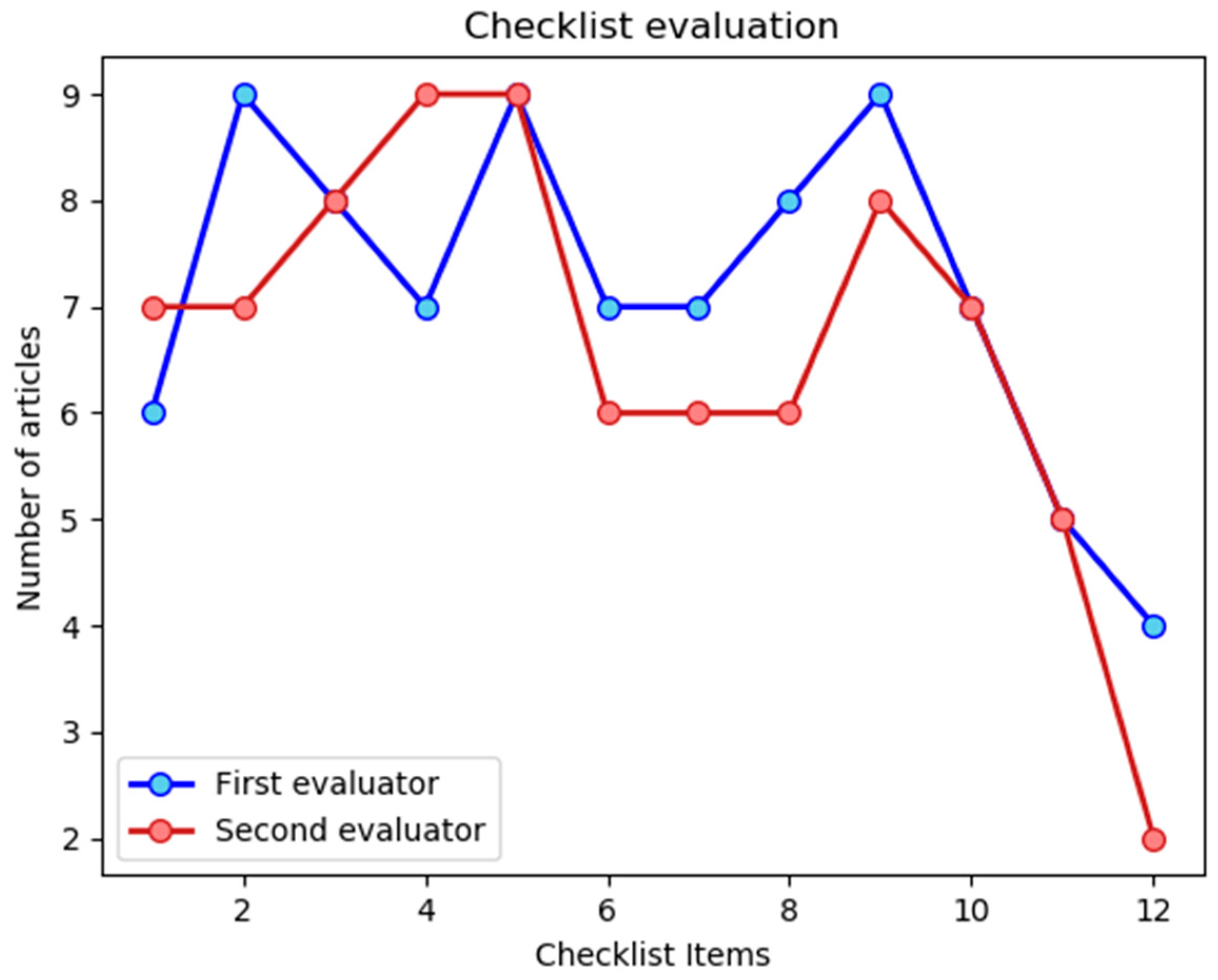
To evaluate the quality of the publications obtained for the review, the items of the checklist shown in Table 1 were considered to compare the content of the publications. The first evaluator provided an average value of 9.56 ± 1.89 out of 12 for the 9 articles, whereas the second evaluator determined an average assessment of 8.89 ± 1.97 out of 12. To assess the concordance on the evaluations, the kappa (κ) value was calculated, which takes into account the effect of chance on the observed agreement, obtaining a value of κ = 0.67. This result indicates a moderate-high level of agreement between the evaluators. To facilitate the analysis on the fulfillment of the checklist items, Figure 2 shows a plot displaying the number of articles that satisfies each of the items.

Regarding the content of the articles selected for this review,

Table 2. Summary of the clinical variables, such as objectives, subjects, EEG recording protocol, EEG cleaning protocol and dataset pre-processing. Acronyms: QEEG—quantitative electroencephalogram; EEG—electroencephalogram; PD—Parkinson’s disease; HC—healthy controls; LD—levodopa; RBD—REM behavior disorder; HY—Hoehn–Yahr scale; UPDRS—unified Parkinson’s disease rating scale; EMG—electromyogram; PET—positron emission tomography—ECG electrocardiogram; EOG—electrooculogram; HOS—higher order spectrum. Here n stands for the number of patients.

Ref.	Objective	Subjects	Sex (F/M)	Age	Hoehn–Yahr (n)	UPDRS	Disease Duration	EEG Parameters	EEG Pre-Processing
[29]	Selection of the best QEEG characteristics to identify different levels of cognitive impairment in PD.	118 PD with LD classified into 5 groups according to the severity of the disease. G1: n = 28, G2: n = 33, G3: n = 43, G4: n = 5, G5: n = 9.	G1 = 8/20 G2 = 9/24 G3 = 16/27 G4 = 3/2 G5 = 0/9	G1 = 60.54 ± 8.75 G2 = 66.09 ± 6.65 G3 = 67.04 ± 7.94 G4 = 73.19 ± 5.29 G5 = 67.56 ± 5.51	G1 = 1.93 ± 0.4 G2 = 2.14 ± 0.55 G3 = 2.21 ± 0.59 G4 = 2.40 ± 0.55 G5 = 2.00 ± 0.97	G1 = 26.00 ± 11.73 G2 = 29.55 ± 12.22 G3 = 28.74 ± 11.44 G4 = 31.00 ± 12.79 G5 = 29.00 ± 18.87	G1 = 7.75 ± 5.29 G2 = 8.36 ± 7.49 G3 = 8.81 ± 5.02 G4 = 6.60 ± 3.58 G5 = 12.00 ± 6.56	122-channel EEG recorded during 10 min in resting state with 512 Hz sampling rate.	Average reference and 0.1–100 Hz bandwidth filter. Ocular artifacts were corrected and a 50 Hz filter was applied. Periods of drowsiness were removed, and the semi-automatic rejection of artifacts was performed to eliminate muscle activity. Each channel was divided into 4 s epochs. At least 20 segments were used for the analysis.
[30]	Selection of the QEEG parameters that best distinguish between controls and PD.	50 PD and 41 controls.	PD: 17/33 HC: 20/21	PD: 68.8 ± 7 HC: 71.1 ± 7	Not specified.	Not specified.	5.3 ± 5.1	256-channel EEG recorded during 12 min in resting state with eyes closed and 500 Hz sampling rate.	Three minutes of EEG were constructed with segments of at least 30 s without artifacts, and a 0.5–70 Hz filter was applied. An inverse Hanning window was used to join segments. It was referenced with respect to mean and defective channels were interpolated with the spherical spline method. “Runica” was used with default settings to remove further artifacts.
[31]	Classification of patients vs. controls for the diagnosis of PD.	20 PD with LD and 20 controls. All right-handed.	PD: 10/10 HC: 11/9	PD: (45–65) HC: 58.1 ± 2.95	1: (2) 2: (11) 3: (7)	Not specified.	5.75 ± 3.52	Fourteen-channel EEG recorded during 5 min in Resting state with 128 Hz sampling rate.	Epochs of 2 s were segmented and a threshold technique was applied at ±100 µV. A sixth order Butterworth band-pass filter was applied with direct reverse filtering technique at 1–49 Hz.
[32]	Classification of patients with RBD and controls. Some of the patients with RBD were eventually diagnosed with PD and dementia.	118 RBD and 74 controls. 14 RBD became PD. No direct patient data.	Not specified.	Not specified.	Not specified.	Not specified.	Not specified.	Fourteen-channel EEG at 256 Hz sampling rate in resting state with open-eye periods followed by closed-eye periods.	The first EEG of each patient was considered baseline. A band-pass filter was passed at 0.3–100 Hz with a notch filter at 60 Hz to minimize the noise from the power line. It was also filtered at 4–44 Hz. The signals were referenced to the ears.
[33]	Classification of patients with PD in the early stages of the disease vs. controls.	30 PD and 30 controls.	Not specified.	PD: (50-70) HC: (50-70)	1–1.5	Not specified.	Not specified.	Two-channel EEG recorded during 30 min for the flexion and extension of the wrist.	Not specified.
[34]	Classification of the patients with PD in the early stages of the disease vs. controls using various algorithms.	100 PD and 100 controls.	Not specified.	PD: (50-70) HC: (50-70)	1–1.5	Not specified.	Not specified.	Two-channel EEG recorded during 30 min for the flexion and extension of the wrist.	5–50 Hz band-pass filter was applied.
[35]	Classification of patients with neurological diseases vs. controls to search for spectral equivalence between various neurological and neuropsychiatric disorders with Thalamocortical dysrhythmia.	31 PD and 264 controls.	PD: 14/17 HC:112/152	PD: 56.62 ± 12.32 HC: 49.51 ± 12.54	1–3	43.44 ± 15.53	Not specified.	Nineteen-channel EEG recorded during 5 min in resting state with eyes closed and 1024 Hz sampling rate.	The data were referenced to the ears, and the impedances were <5 kΩ at all electrodes during the recording. High-pass filter at 0.15 Hz and low-pass filter at 200 Hz were used. Data were resampled at 128 Hz, and band-pass filtered at 2–44 Hz. Artifacts were manually removed.
[36]	Classification of PD and controls to demonstrate the utility of EEG as biomarker for PD.	21 PD (18 for DAT PET) OFF LD during 12 h and 25 controls (24 for DAT PET).	PD: 7/14 HC: 9/16	PD: 62.7 ± 7.32 HC: 54.6 ± 10.5	2.07 ± 0.39	PD: 31.00 ± 10.37 HC: 0.83 ± 1.27	Not specified.	Twenty-channel EEG and 4 additional channels for ECG, EMG or EOG. Two recordings per patient are recorded during 5 min in resting state with eyes closed and 256 Hz sampling.	Not specified.
[37]	Selection the best classifier of PD vs. controls using the minimum number of HOS features.	20 PD with LD and 20 Controls. All right-handed.	PD: 10/10 HC: 11/9	PD: 59.05 ± 5.64 HC: 58.10 ± 2.95	1: (2) 2: (11) 3: (7)	Not specified.	5.75 ± 3.52	Fourteen-channel EEG recorded during 5 min in resting state with eyes closed and 128 Hz sampling rate.	Threshold technique at 80 µV. Butterworth sixth-order band-pass filter at 1–49 Hz. Each channel is separated into 2 s epochs with 50% overlap.

and

Table 3. Summary of the model parameters, such as features extracted, models used, model architecture, training and validation methods, results and metric used for the articles included in this review. The columns with the references and objectives of the selected articles are included again for the sake of readability. Acronyms: EEG—electroencephalogram; PD—Parkinson’s disease; FFT—fast Fourier transform; ROI—regions of interest; SVM—support vector machine; KNN—K-nearest neighbors with k being the number of nearest neighbors considered; LR—logistic regression; LASSO—least absolute shrinkage and selection operator; ROC—receiver operating characteristic; AUC—area under the curve; CNN—convolutional neural network; RNN—recurrent neural network; LSTM—long-short term memory network—GRU—gated-recurrent unit—MLP—multilayer perceptron; DT—decision tree; RF—random forest; RBF—radial basis function; EMG—electromyogram; ANN—artificial neural network; PET —positron emission tomography; DFA—discriminant function analysis; FKNN—fuzzy K-nearest neighbors with m being the fuzzy strength parameter; NB—naïve Bayes; PNN—probabilistic neural network with σ being the smoothing parameter; PPV—positive predictive value; NPV—negative predictive value; HOS—higher order spectrum. Here n stands for the number of patients.

Ref.	Objective	Features	Models	Model Parameters	Training	Validation Strategy	Metrics	Best Result
[29]	Selection of the best QEEG characteristics to identify different levels of cognitive impairment in PD.	The relative and absolute spectral power was obtained for each epoch using a FFT and a 50% overlap for the Delta, Theta, Alpha and Beta bands. Moreover, a division into 5 ROI was performed. For each case, high and low electrode density were considered. A statistical dependency study with an analysis of variance and the selection of characteristics with Pearson’s correlation method was carried out.	SVM, KNN	SVM: Gaussian kernel KNN: k = 9 and the Euclidean distance as a metric.	The dataset is randomly split into k-fold (for this case k = 5). k-1-folds were used to train the models and the rest fold was the testing set. The dataset used for the k-fold cross-validation was the set with n = 100.	Two validation strategies. First: divide the full dataset into training set with n = 100 and validation set with n = 18. Second: the training set was used for 5-fold cross-validation.	Accuracy.	SVM: Accuracy = 87 ± 3.5 KNN: Accuracy = 88 ± 2.8 Both were achieved for the relative power with low-electrode density. Groups with few patients had worse results.
[30]	Selection of the QEEG parameters that best distinguish between controls and PD.	Ten brain regions were considered with 79 different measurements. All of the features were extracted from the frequency spectrum.	RF, SVM, DT, LR and LR with LASSO	SVM: Non-linear kernels such as RBF were used.	A 10-fold cross-validation was considered and optimization was carried out for tuning parameters.	A 10-fold cross-validation.	Accuracy, AUC.	The most significant models were: RF: Accuracy = 78 AUC = 0.8 LR with LASSO: AUC = 0.76
[31]	Classification of patients vs. controls for the diagnosis of PD.	There was no pre-processing of data.	CNN	Thirteen layers with 4 1D convolution layers, 4 max-pooling layers and 3 fully connected layers. Adam optimizer (learning rate = ${10}^{-4}$). Activation function Relu and the last one Softmax. Dropout of 0.5.	A 10-fold cross-validation with 9 parts for training and 1 for testing; 20% of the training data were also used for validation.	Two validation strategies. First: 10-fold cross-validation with all the data. Second: 20% of the training data were also used for validation at the end of each epoch.	Accuracy, sensitivity, specificity.	CNN: Accuracy = 88.25, sensitivity = 84.71, specificity = 91.77
[32]	Classification of patients with RBD and controls. Some of the patients with RBD were eventually diagnosed with PD and dementia.	Several spectrograms per subject were generated, each of them of 20 s and artifact-free, until about 2.5 min per patient was obtained. The data were centered and normalized to unit variance.	CNN, RNN	CNN: 4 hidden-layer convolutional net with pooling. Dropout was used as regularization, max-pooling layers and using a cross-entropy loss function. RNN: with LSTM and GRU, with 3 cells which 32 units each. Dropout was used.	For training, datasets were balanced by random replication preserving the distribution of the subjects.	Leave-pair out (LPO) cross-validation, where one subject from each class was left out for validation.	Accuracy, AUC.	The results for controls vs. PD: CNN: Accuracy = 79 ± 1 AUC = 0.87 ± 0.1 RNN: accuracy = 81 ± 1 AUC = 0.87 ± 0.1 In RNN, there was no difference between LSTM and GRU.
[33]	Classification of patients with PD in the early stages of the disease vs. controls.	EEG: Shannon entropy, Lyapunov and inverse Lyapunov exponent were calculated. EMG: power, standard deviation, root mean square, variance, waveform length, modified median, and mean frequency.	MLP	Back Propagation was used as the learning algorithm and ‘trainlm’ was used as the training function. Sigmoid transfer function was used for the hidden layer.	The dataset was divided into: training 70%, validation 15% and testing 15%.	Validation with validation and test sets.	Accuracy.	MLP with inputs: EEG: accuracy = 62 EMG: accuracy = 73 EEG+EMG: accuracy = 98.8
[34]	Classification of patients with PD in the early stages of the disease vs. controls using various algorithms.	EEG: Lyapunov and inverse Lyapunov exponent, Shannon entropy. EMG: power, Standard deviation, root mean square, variance, waveform length, modified median, and mean frequency.	MLP	3 algorithms were tested: Gradient Descent algorithms (traingd, traingdm), Conjugate Gradient algorithms (traininscg, traincgp), and Quasi-Newton algorithms (trainbfg, trainlm). Sigmoid function was used in the hidden layer. The number of hidden neurons was checked for 5, 7, 9,10,20,30.	The dataset was divided into: training 70%, validation 15% and testing 15%.	Validation with validation and test sets.	Accuracy RMSE, R value.	ANN with Trainlm and 10 neurons: accuracy = 100 RMSE = 4.03 × 10−3 R value = 0.9998
[35]	Classification of patients with neurological diseases vs. controls to search for spectral equivalence between various neurological and neuropsychiatric disorders with Thalamocortical dysrhythmia.	The power spectrum was calculated for each subject and the five frequency bands (delta, theta, alpha, beta, and gamma) were considered for each ROI.	SVM	The default settings were used as the running parameters.	A 10-fold cross-validation was performed on the full dataset with 90% of the data for training and 10% of the data for testing. The distribution of the patients was kept.	A 10-fold cross-validation. Moreover, controls with obesity were used to validate the model.	Accuracy, TPR, FPR, ROC, MAE, RMSE.	The results for controls vs. PD: accuracy = 94.34 ± 1.81 TPR = 0.93 ± 0.02 FPR = 0.11 ± 0.01 ROC = 0.95 ± 0.02 MAE = 0.07 ± 0.02 RMSE = 0.16 ± 0.02
[36]	Classification of PD and controls to demonstrate the utility of EEG as a biomarker for PD.	Coherence analysis with 2 s windows with 50% overlap was carried out. Pearson’s correlation was calculated to assess the relationships between coherence and disease severity. The relative and absolute PSD was calculated at 1–40 Hz. Only 14 EEG-based features were finally used.	DFA	A linear DFA was used to build the classifier. The classifier input was selected by utilizing the step-wise discriminant analysis procedure in the SPSS software package.	Not specified.	Cross-validation.	Accuracy, sensitivity, Specificity, PPV (precision), NPV.	Accuracy = 95.24 sensitivity = 94.74 Specificity = 95.65 PPV = 94.74 NPV = 95.65 An excessive coherence was observed in the Beta and Gamma bands for PD.
[37]	Selection the best classifier of PD vs. controls using the minimum number of HOS features.	For each epoch, a total of 13 HOS characteristics were calculated. The Student’s t-test was also obtained to determine the importance of the characteristics.	DT, KNN, FKNN, NB, PNN, SVM	FKNN: Euclidean distance, m = 1.24 and k = 3. KNN: k = 2 and Euclidean distance. PNN: exponential activation function and σ = 0.284. SVM: polynomial kernel functions of order 2 and 3, RBF and linear kernels.	The characteristics were added one by one to each classifier until maximum precision is achieved.	A 10-fold cross-validation.	Accuracy, sensitivity, specificity, precision, F-score.	The best model was SVM with RBF kernel: accuracy = 99.62 ± 0.58 sensitivity = 100 ± 0.0 specificity = 99.25 ± 0.53 precision = 99.38 ± 0.47 F-score = 0.98 ± 0.05

below show a summary with their characteristics, from the clinical and computer sciences points of view, respectively, providing a qualitative analysis of the checklist items in Table 1. The aspects that were extracted included: 1. analysis of the quality of the dataset, through the study of the number of patients recruited, the type of EEG recording performed and its parameters. 2. analysis of the pre-processing of the data, through the EEG cleaning protocol used and the features extracted from the EEG, if any. 3. characteristics of the model utilized, specifying if one or more models were used, the parameters of the model architecture and the training and validation methods used. Table 3 includes an additional column with the most relevant results obtained in each of the articles, allowing the analysis of the most representative model parameter pairs for this study.

The information summarized in Table 2 and Table 3 facilitates the comparison between the different articles and the properties of the studies carried out in each of them. Regarding the objective of the selected articles, eight of them studied classification problems, which seek for the diagnosis of PD by distinguishing between patients with PD and healthy patients or controls. The remaining article classified the degree of cognitive decline of PD.

The balance between the number of patients with PD and controls is crucial when using ML techniques, because unbalanced data can lead to errors in prediction. It can be verified that this was a common practice in the reviewed articles, since seven of the eight articles that classified PD considered a balanced dataset. Regarding the number of patients included in the studies, it should be noted that studies with less than 50 patients in each category predominated, with an average value of 28.20 ± 11.53 for the group of patients with PD and an average value of 27.20 ± 7.83 for the controls. The articles did not indicate whether the number of patients was adequate for the classification problem. Moreover, although the average value of the age of both groups was not specified in all the articles, it was a general practice in all of them to take patients with PD aged between 45 and 70 years, with a mean value oscillating around 60 years, which corresponds to the age of incidence of the disease. On the other hand, the healthy patients, or controls, were chosen so that they exhibited the same demographic characteristics as the group of patients with PD. It is worth noting that only four of the selected articles indicated whether the patients had taken their dose of levodopa (three studies performed the EEG in ON state, one in OFF state).

Regarding the degree of the progression of the disease, a general lack of data can be noticed according to the information summarized in Table 2. Only six articles specified the status of the patients according to the Hoehn–Yahr (HY) scale, four of them considered HY: 1–3, and two of them only considered patients in early stages of the disease (HY 1 and 1.5). None of them included patients in the most advanced phases of the disease, which may be a limitation to evaluate the ability of the results to be extrapolated or evaluate the disease progression. Similarly, only three articles showed the state of the patients according to the UPDRS, with an average value of 34.43 ± 6.43. The duration of the disease was specified in four articles, with an average value of 6.38 ± 1.35 years.

With respect to the parameters of the EEG recording, one may notice that the number of EEG channels varied among the different studies. An EEG recording with a high density of electrodes (greater than 100) was used in two articles, whereas a low density of electrodes (fewer or equal than 20) was considered in five articles with an average value of 16.2 ± 2.72 electrodes. The remaining two articles used EEG recordings with only two channels, which they considered a technique that combined both EEG and EMG. It should be remarked that these articles were related to the same study, carried out by the same research group. The EEG recording time was also variable between the articles, showing heterogeneous values again. The test mostly performed with a duration of 5 min, which appeared in four articles.

Regarding the pre-processing, it is possible to distinguish between the EEG cleaning protocol (shown in Table 2), and the feature extraction from the dataset (shown in Table 3). The EEG pre-processing, or EEG cleaning, varied from one article to another, mainly due to the lack of a standard EEG cleaning protocol. This makes it difficult to assess the quality of the dataset. In particular, three of the articles performed the EEG pre-processing by removing signal artifacts, three articles minimized the signal noise through the filters, and the remaining three articles did not specify the cleaning process, which leads us to think that no alteration in the EEG signals was carried out. On the other hand, associated with the dataset pre-processing for the input of the model, it should be remarked that the features extracted from EEG signals were very different in between the articles. However, all of them were extracted from the frequency spectrum, and there was only one article in which no data pre-processing was performed.

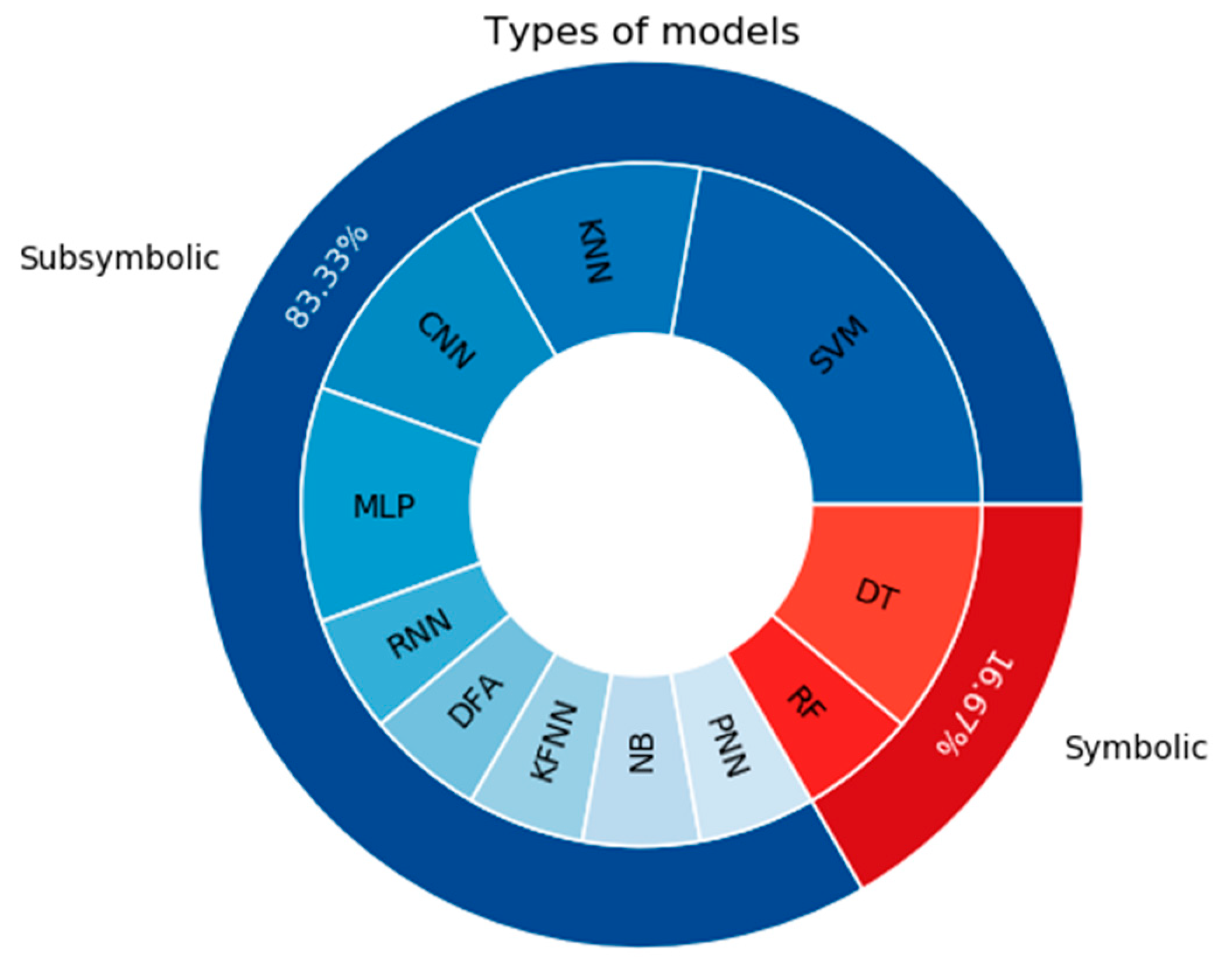
Regarding the ML models, as shown in Table 3, the nine selected articles made use of a total of 11 different ML techniques in order to carry out the classification problems to distinguish patients with PD and controls. The number of techniques exceeds the number of articles due to the fact that, whereas in five articles, a unique model was considered, in the remaining four articles, different techniques were compared. Concerning the type of processing, it is worth noting that the models associated with a subsymbolic processing predominated over those related with a symbolic one.

To conclude this analysis of the information summarized in the Table 2 and Table 3, it should be pointed out the great heterogeneity between the articles from the point of view of the model used and the absence of a baseline that allows the comparison between the different studies, making it especially difficult to discuss the information displayed in the model parameters and validation columns. The results obtained in each article will be discussed in the subsequent sections of this review.

3.3. Types of Models Considered

One of the most notable characteristics of the selected articles has to do with the variety of models used. Figure 3 shows a pie chart with the different models and the number of times they were considered in the articles. These models are: support vector machine (SVM), K-nearest neighbors (KNN), decision tree (DT), convolutional neural network (CNN), multilayer perceptron (MLP), random forest (RF), recurrent neural network (RNN), discriminant function analysis (DFA), fuzzy K-nearest neighbors (FKNN), naïve Bayes (NB) and probabilistic neural network (PNN). It can be noticed from Table 3, and more specifically from Figure 3, that the number of models used exceeds the number of articles. This follows, as a consequence of the fact that four of the selected articles compared the results offered by different models, whereas five of them considered a single model.

Concerning the type of processing associated to the models, both DT and RF belong to the group of symbolic models, whereas the remaining ones are subsymbolic. Hence, despite the diversity of the ML models considered, those whose processing was subsymbolic predominated. As an individual technique, SVM was the mostly used one, and as it will be seen later, it provided the best results for classifying patients with PD vs. healthy controls. On the other hand, it is worth emphasizing the fact that artificial neural networks (ANN) also played an important role in the reviewed articles since these techniques were used six times through CNN, MLP, RNN and PNN. Note that one of the articles considered two different models associated with RNN, with LSTM and GRU layers, respectively, as shown in Table 3, although this has not been taken into account, neither in Figure 3, nor in the previous computation.

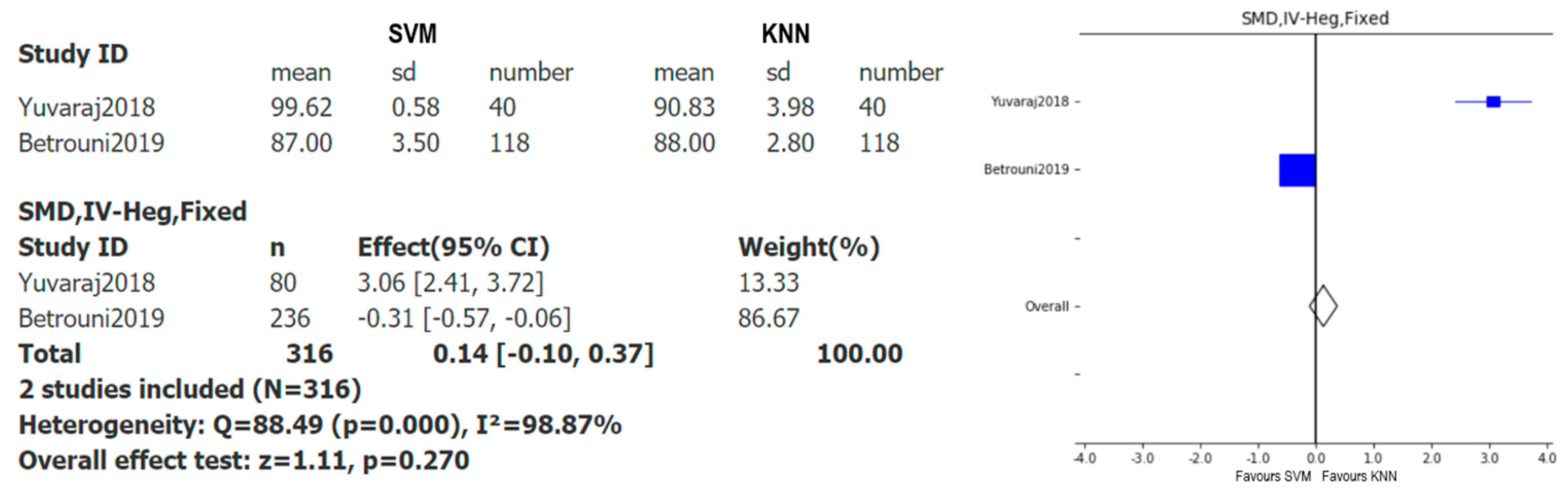
Taking into account that the most used models were SVM and KNN and the most used metric was accuracy, a comparative study between both models was carried out through a forest plot. To perform this analysis, it is necessary that several studies use these two models, and only two articles satisfied this condition [29,37], respectively. Figure 4 shows the meta-analysis with the results of the accuracy of both models, for the choice of standard mean difference (SMD) for the effect measure, inverse variance Hedges’ adjusted g for the algorithm, and fixed models for the effect models considered.

As pointed out before, this plot shows the (standardized) difference of the means of SVM and KNN data. Thus, it favors the results with smaller values of the accuracy. For instance, in the first article, the lowest accuracy value was obtained by KNN and in the second article by SVM. Since the difference between both models is greater in the first article, the confidence interval (CI) is far away from zero, whereas in the case of the second article, as the values of the means are close to each other, the CI is close to zero. From the information shown in Figure 4, the difference between the number of subjects considered in each of the studies and how much the meta-analysis is affected by this fact become particularly noticeable. It is particularly striking how the sample size influences both the CI and the weight in each case. Indeed, the larger the number of patients, the smaller the amplitude of the CI, and the greater the weight. Since none of the confidence intervals crosses the ‘no effect line’, the difference between the models’ SVM and KNN is statistically significant in both studies. However, as the overall result, the meta-analysis shows that there is no statistically significant benefit of choosing one model over the other, since the diamond crosses the ‘no effect line’. One needs to keep in mind that only two articles are being compared, and that the meta-analysis exhibits a great heterogeneity, which makes the represented data less conclusive. Hence, more studies considering both ML models simultaneously are needed to provide a more reliable objective conclusion. Finally, it is worth emphasizing that, although ML techniques are influenced by the amount of data introduced to the model, this does not imply that models with more data always give better results, but it is crucial that the training set is sufficiently large for the study.

3.4. Type of EEG Recording

As can be seen in Table 2, the selected articles considered two types of EEG records. Therefore, the articles have been divided into two categories based on the EEG tests performed. On the one hand, the resting state EEG group corresponds to articles [29,30,31,32,35,36,37], for which the EEG was recorded in the resting state. On the other hand, the motor action EEG group corresponds to articles [33,34] which recorded the EEG by means of a motor activation test, specifically a wrist extension and flexion test. For each of these articles, the model considered, the classification results obtained, the characteristics introduced, and the type of EEG cleaning performed are shown in

Table 4. Summary of the results, features introduced to the models and signal filtering shown in Table 2 and Table 3 for the selected articles. The year of publication of each article has been added. Acronyms: ANN—artificial neural network; DFA—discriminant function analysis; EEG—electroencephalogram; EMG—electromyogram; SVM—support vector machine; KNN—K-nearest neighbors; CNN—convolutional neural network; RNN—recurrent neural network.

Ref	Year	Accuracy Results	Features	Artifacts
[29]	2019	84%—SVM and 88%—KNN	Relative power low-electrode density	Free-artifact
[30]	2017	78%—random forest	Selects the most important characteristics	Free-artifact
[31]	2018	88.25%—CNN	Not considered	Noise filter
[32]	2019	79%—CNN and 81%—RNN	Spectrogram	Noise filter
[33]	2019	EEG—62%, EMG—73%, and both combined—98.8%	EEG: non-lineal parameters. EMG: statistical parameters.	Not specified
[34]	2019	ANN 100% with the quasi-Newton algorithm Trainlm	EEG: non-lineal parameters. EMG: statistical parameters.	Not specified
[35]	2018	94.34%—SVM	Power spectra of bands and regions	Free artifact
[36]	2020	95.24%—DFA	Coherence in the beta band	Not specified
[37]	2018	99.62%—SVM	Features of the higher-order spectra	Noise filter

.

3.4.1. Resting State EEG Group

The resting state EEG group contains seven articles, which considered different measurement protocols and channels of the EEG recording. Articles [31,37] were based on the same study but using different features and models, as it can be seen in Table 3. The predominant protocol within this group consisted of recording the EEG in the eyes closed resting state, which was used in four articles. On the other hand, the articles exhibited different recording durations, with an average value of 6.37 ± 3.10 min, and a mode of 5 min, which was considered in four of the seven articles of this group. The number of EEG channels also varied inside the resting group, with a low density of electrodes prevailing: 71.43% of these articles considered between 14 and 20 electrodes, whereas in the rest the number of channels exceeded 100 electrodes.

Data pre-processing can be divided into two categories, which are EEG pre-processing or EEG cleaning, and data pre-processing or EEG feature extraction. Regarding EEG cleaning, it can be concluded from the summary displayed in Table 4 that there was no standard cleaning protocol, because the EEG was left free of artifacts in three articles, whereas three of the remaining articles only performed a pre-processing with filters to reduce the noise in the signals (artifacts were not eliminated). The protocol was not specified in [36]. On the other hand, regarding the extraction of features, only in [31] the EEG signal was introduced to make a morphological analysis, whereas in the remaining articles, different spectral characteristics were calculated.

The results in Table 4 show that both SVM and DFA, considered by articles [35,36,37], were the models that provided better classification results (accuracy greater than 90%) for patients with PD vs. controls. Note that [36] recorded the EEG of patients with PD without Levodopa intake. These articles introduced different features of the frequency spectrum into the network and performed different EEG cleaning protocols. On the other hand, [29], which also used SVM, did not classify patients with PD vs. controls, but studied the disease progression. Thus, the precision obtained for that case is not comparable with that of the others.

To conclude, in this group, the evaluation of the quality criteria according to the checklist of Table 1 provided an average value of 10.43 ± 1.05 out of 12 according to the first evaluator and a value of 9.71 ± 1.28 out of 12 according the second one. The kappa value calculated for the items in this group was 0.71. It can be appreciated that this value is higher than the one obtained when considering all the selected articles. This indicates that the evaluators exhibit a greater agreement when restricting to the articles of the resting state EEG group.

3.4.2. Motor Action EEG Group

Only two articles performed motor action tests. Actually, they were based on the same study. Therefore, in both of them, two channels of EEG and EMG were recorded for 30 min, in a test of motor activation in which the wrist was extended and flexed. The same non-linear parameters were calculated, although the parameters introduced into the network changed in each article. EEG pre-processing was not specified. In both cases, ANN was used but for different purposes. In [33], three studies were made to select the input parameters to the model that provided the best results, whereas in [34], six different techniques were studied for the same input parameters with the aim of selecting the best model. Moreover, in [34], the input features were a combination of EEG and EMG coinciding with the parameters that provided better results in [33]. The summary of the motor group results is shown in Table 4.

According to the checklist in Table 1, the articles received an assessment of 6.5 ± 0.5 out of 12 by the first evaluator and 6 ± 1.0 out of 12 by the second one. The kappa value for this group was 0.58. In this case, it can be appreciated that the resulting kappa value is slightly lower than the ones obtained for the resting state EEG group and for the global set of articles, which indicates a lower agreement between the evaluators with respect to previous cases.

4. Discussion

PD is a disease mainly characterized by motor dysfunctions which affects the quality of life of patients. The application of ML techniques in EEG may be able to identify diagnostic and progression markers with the potential to be applied in the clinical setting through a simple quick-to-perform test, with a low error rate and at low cost and invasiveness. It can be observed that the oldest article of the nine selected in this review was just three years old, and the number of articles has increased in the following years, showing the novelty and growing development of ML techniques applied in EEG in relation to PD. On the other hand, regarding the global distribution of the selected articles, it can be appreciated that, according to the first affiliation country of the first author, although Asia stands out as the continent with the highest number of publications, the distribution is relatively homogeneous between the continents of Asia, Europe and North America, reflecting a global interest in encompassing the objectives of this review.

To assess the quality of the selected articles and facilitate the comparison between them, the content of each article was evaluated using the checklist of the guidelines for developing and reporting machine learning predictive models in biomedical research [28]. This evaluation was carried out by two different evaluators and obtained an average value of 9.56 ± 1.89 out of 12, and 8.89 ± 1.97 out of 12, respectively, which indicates the good quality of the included articles. The kappa value among the two independent reviewers was calculated, obtaining a value of 0.67, which indicates a substantial agreement between the evaluations. Both evaluators agree that the less fulfilled items were 11 and 12, which are related to the limitations of the model and the unexpected results, respectively. The fact that most of the articles did not include this kind of analysis may be due to the fact that sometimes the scope or limitations were unknown at the time of publication and they only became evident over the years and with the development of new algorithms.

Among the different clinical variables studied by the articles, it becomes apparent that a lack of clinical parameters was associated to the state of the PD. As it can be noticed from Table 2, variables like the degree of disease progression according to the HY scale, the state of the disease according to the UPDRS, and the years of duration of the disease, were not provided by all the articles. The lack of information about these variables can influence the classification results and lead to false positives/negatives. For instance, if a binary classification network (Parkinson vs. no Parkinson) is trained with patients in advanced stages of the disease, it may be the case that the model misclassifies a patient with PD in the early stage of the disease. It would be interesting to further evaluate these data, since a classifier may work differently with patients in different phases of the disease. Actually, it should be noted that only [29] did a study classifying the degree of progression of the disease, in which the groups with more advanced stage patients obtained worse results in the classification, nevertheless, these groups were the smaller ones (less than 10 subjects) meanwhile the rest of the stages with better results had more than 20 subjects. ML techniques require a large enough dataset to work properly, so these results suggest that small groups of patients are not sufficient for the model used in that study (SVM). Furthermore, we did not find information in all the articles regarding the medication taken by the subjects, despite the fact that dopaminergic drugs are known to influence the EEG characteristics and therefore vary the classification results. Finally, on the side of the ML models, the information incorporated in the articles is more abundant and homogeneous. However, it stands out that the absence of metrics associated to the area of medicine and the clinical setting, such as sensitivity, specificity, true positives, etc. The lack of both these metrics and information concerning the state of the patient lead us to think about the necessity for new translational studies that incorporate these variables.

Regarding the quality of the EEG signals, it is conditioned both by the EEG recording parameters and by the EEG acquisition protocol. Within the recording of the EEG signals, although the number of electrodes and the duration of the EEG test vary among articles, they do not affect the quality but rather the spatial resolution of the EEG signal, which is outside the scope of this review. Nevertheless, although the number of electrodes does not affect the quality of the signal, a high density of electrodes may benefit the study of some neurological diseases with a widespread pattern of involvement in the brain. Furthermore, there are parameters of the EEG recording, such as the sampling frequency, that can affect the result obtained from the variables calculated from the EEG, and therefore can influence the quality of the study. Finally, since PD is characterized by motor dysfunctions, it is striking that the resting state tests predominated over the tests associated with motor activation, such as the finger tapping test or the wrist extension and flexion test, which were only considered only in two of the selected studies. This may be caused by the influence of the abundant publications available of neuroimaging studies on the resting state in neurological diseases as PD.

In the articles of this review, two types of data pre-processing were evaluated, which are the cleaning of the EEG and the extraction of EEG characteristics. As can be seen in Table 2, there was no standard cleaning protocol for the EEG. This makes it difficult to perform an evaluation of the dataset, since it is not possible to evaluate the loss of elements in the EEG and how these affect the results of the classification problem. As shown in Table 3, there was also a great heterogeneity in the features that were extracted from the EEG. However, it should be noted that spectral characteristics predominated. This may be due to the fact that the spectral features provide information on variations in the EEG bands, and alterations in these bands provide more clinical information than a morphological analysis of the signal, especially in Parkinson’s disease, where visual alterations in the EEG signals of patients with PD are not observed.

To evaluate how the extraction of features affects the accuracy of the model, we must take into account the architecture of the ML model used. ML techniques allow the analysis of large amounts of data, as well as the extraction of essential characteristics from them. Hence, the choice of the model is influenced both by the size of the dataset and the nature of the data. In the case of this review, the dataset of the selected articles was composed of EEG, and the subsymbolic models are precisely those designed to estimate relationships among data. For this reason, one may expect the subsymbolic models to be the most used ones. This was confirmed by the summary shown in Table 3 and more specifically, by Figure 3. Furthermore, in both of them, it can be appreciated that the most widely used techniques, within subsymbolic processing, were those classified as ANN, i.e., CNN, MLP, RNN and PNN. However, these techniques require a large amount of data for their training, and since in the medical field it is more difficult to obtain data to constitute the dataset, this may justify that the most used individual model was SVM. It is worth emphasizing that ML techniques are continuously growing, and given the novelty of this field of study, there is still a lack of applications for the most complex and novel techniques (like CNN and RNN), which have only been considered in a small number of studies.

To conclude, let us discuss how the extracted features and the cleaning protocol may influence the classification results of the computational models. As can be seen in Table 4, when comparing the articles [35,37], both used SVM with results of an accuracy of 94.34 and 99.62%, respectively. Furthermore, in both of them, different spectral characteristics were introduced and they both considered different EEG cleaning protocols, with [37] being the one that obtained the highest precision by performing less EEG processing. This could lead us to think that EEG processing may be unnecessary when using ML techniques. On the other hand, when comparing the articles [31,32], it can be seen that both used CNN with accuracies of 88.25 and 79%, respectively. Moreover, Table 4 shows that [31,32] carried out similar EEG processing whereas they introduced different features into the models. Furthermore, they considered a different model architecture, the one that obtained the best results being the most complex model. This could indicate that both the parameters that define the model and the characteristics introduced are decisive for obtaining a better performance in the classification problem. The combination of these factors can be appreciated in articles [33,34], since [33] studied the changes in precision when varying the input parameters of the network, whereas [34] analyzed the changes in precision by varying the model parameters. In both cases, very different values were obtained in the PD classification results, which indicates that both the extraction of features and the model parameters are decisive for the study of PD through ML techniques for the analysis of EEG. Hence, the search for a balance between both parameters becomes essential for the development of a precise model that classifies PD.

5. Conclusions

Machine learning techniques play a fundamental role in data analysis, allowing one to obtain patterns and relationships between different classes automatically and efficiently. These techniques are increasingly being applied to EEG analysis, facilitating the use of this low-cost clinical test to detect or extract information on various neurological diseases. Despite the limited number of articles found, it can be noticed that the studies using the resting state tests to classify PD predominate, emphasizing a lack of studies using motor activation tests as well as studies focused on the progression of the disease. There is a great heterogeneity in the data provided by the articles, with a lack of clinical variables such as the use of medication during the recordings and the stage of the disease. In general, the size of the datasets considered in the studies is relatively small compared to the one usually found in the ML literature. However, the selected articles exhibited good results in the classification problem, with values higher than 90% in various studies. A further analysis of the models considered in these articles indicated that both the features introduced into the model and its architecture were essential for a good performance in predicting the classification. On the contrary, the cleaning protocol of the EEG, which was highly heterogeneous among the different studies, did not influence the results, and thus it could be omitted. Since this cleaning process is usually carried out manually, omitting it would benefit the development of an efficient and fast automatic prediction model. Finally, it should be emphasized that ML techniques have experienced significant growth in recent years, incorporating more complex models, and thus, this review and the conclusions obtained herein should be considered as a first step in the analysis of the role played by ML techniques and EEG in the study of PD.

References

- Mahlknecht, P.; Krismer, F.; Poewe, W.; Seppi, K. Meta-Analysis of Dorsolateral Nigral Hyperintensity on Magnetic Resonance Imaging as a Marker for Parkinson’s Disease. Mov. Disord. 2017, 32, 619–623. [Google Scholar] [CrossRef]
- Dickson, D.W. Neuropathology of Parkinson disease. Parkinsonism Relat. Disord. 2018, 46 (Suppl. 1), S30–S33. [Google Scholar] [CrossRef]
- Kalia, L.V.; Lang, A.E. Parkinson’s Disease. Lancet 2015, 386, 896–912. [Google Scholar] [CrossRef]
- Jankovic, J. Progression of Parkinson Disease: Are We Making Progress in Charting the Course? Arch. Neurol. 2005, 62, 351–352. [Google Scholar] [CrossRef] [PubMed]
- Beitz, J.M. Parkinson’s Disease: A Review. Front. Biosci. 2014, S6, 65–74. [Google Scholar] [CrossRef]
- Bigdely-Shamlo, N.; Mullen, T.; Kothe, C.; Su, K.-M.; Robbins, K.A. The PREP pipeline: Standardized preprocessing for large-scale EEG analysis. Front. Neuroinform. 2015, 9, 1–20. [Google Scholar] [CrossRef]
- Cole, S.; Voytek, B. Cycle-by-cycle analysis of neural oscillations. J. Neurophysiol. 2019, 122, 849–861. [Google Scholar] [CrossRef]
- Sorensen, G.L.; Jennum, P.; Kempfner, J.; Zoetmulder, M.; Sorensen, H.B.D. A Computerized Algorithm for Arousal Detection in Healthy Adults and Patients with Parkinson Disease. J. Clin. Neurophysiol. 2012, 29, 58–64. [Google Scholar] [CrossRef]
- Samuel, A.L. Some Studies in Machine Learning Using the Game of Checkers. II-Recent Progress. In Computer Games I; Levi, D.N.L., Ed.; Springer: New York, NY, USA, 1988; pp. 366–400. [Google Scholar] [CrossRef]
- Litjens, G.; Kooi, T.; Bejnordi, B.E.; Setio, A.A.A.; Ciompi, F.; Ghafoorian, M.; Sánchez, C.I. A survey on deep learning in medical image analysis. Med. Image Anal. 2017, 42, 60–88. [Google Scholar] [CrossRef] [Green Version]
- Jiang, F.; Jiang, Y.; Zhi, H.; Dong, Y.; Li, H.; Ma, S.; Wang, Y. Artificial intelligence in healthcare: Past, present and future. Stroke Vasc. Neurol. 2017, 2, 230–243. [Google Scholar] [CrossRef]
- Miller, D.D.; Brown, E.W. Artificial Intelligence in Medical Practice: The Question to the Answer? Am. J. Med. 2018, 131, 129–133. [Google Scholar] [CrossRef] [PubMed]
- Gandal, M.J.; Edgar, J.C.; Klook, K.; Siegel, S.J. Gamma synchrony: Towards a translational biomarker for the treatment-resistant symptoms of schizophrenia. Neuropharmacology 2012, 62, 1504–1518. [Google Scholar] [CrossRef] [PubMed] [Green Version]
- Sleigh, J.W.; Olofsen, E.; Dahan, A.; de Goede, J.; Steyn-Ross, A. Entropies of the EEG: The effects of general anaesthesia. In Proceedings of the 5th International Conference on Memory, Awareness and Consciousness, New York, NY, USA, 1–3 June 2001; Available online: https://researchcommons.waikato.ac.nz/handle/10289/770 (accessed on 23 January 2019).
- Kannathal, N.; Choo, M.L.; Acharya, U.R.; Sadasivan, P.K. Entropies for detection of epilepsy in EEG. Comput. Methods Programs Biomed. 2005, 80, 187–194. [Google Scholar] [CrossRef] [PubMed]
- Roy, Y.; Banville, H.; Albuquerque, I.; Gramfort, A.; Falk, T.H.; Faubert, J. Deep learning-based electroencephalography analysis: A systematic review. J. Neural Eng. 2019, 16, 1–37. [Google Scholar] [CrossRef]
- Sheng, J.; Wang, B.; Zhang, Q.; Liu, Q.; Ma, Y.; Liu, W.; Shao, M.; Chen, B. A novel joint HCPMMP method for automatically classifying Alzheimer’s and different stage MCI patients. Behav. Brain Res. 2019, 365, 210–221. [Google Scholar] [CrossRef]
- Raghavendra, U.; Acharya, U.R.; Adeli, H. Artificial Intelligence Techniques for Automated Diagnosis of Neurological Disorders. Eur. Neurol. 2019, 82, 41–64. [Google Scholar] [CrossRef]
- Jahmunah, V.; Oh, S.L.; Rajinikanth, V.; Ciaccio, E.J.; Cheong, K.H.; Arunkumar, N.; Acharya, U.R. Automated detection of schizophrenia using nonlinear signal processing methods. Artif. Intell. Med. 2019, 100, 101698. [Google Scholar] [CrossRef]
- Chen, Y.; Gong, C.; Hao, H.; Guo, Y.; Xu, S.; Zhang, Y.; Yin, G.; Cao, X.; Yang, A.; Meng, F.; et al. Automatic Sleep Stage Classification Based on Subthalamic Local Field Potentials. IEEE Trans. Neural Syst. Rehabil. Eng. 2019, 27, 118–128. [Google Scholar] [CrossRef]
- Zhou, M.; Tian, C.; Cao, R.; Wang, B.; Niu, Y.; Hu, T.; Guo, H.; Xiang, J. Epileptic Seizure Detection Based on EEG Signals and CNN. Front. Neuroinform. 2018, 12, 95. [Google Scholar] [CrossRef] [Green Version]
- Dhivya, S.; Nithya, A. A Review on Machine Learning Algorithm for EEG Signal Analysis. In Proceedings of the 2018 Second International Conference on Electronics, Communication and Aerospace Technology (ICECA), Coimbatore, India, 29–31 March 2018; pp. 54–57. [Google Scholar] [CrossRef]
- Rasheed, K.; Qayyum, A.; Qadir, J.; Sivathamboo, S.; Kwan, P.; Kuhlmann, L.; O’Brien, T.; Razi, A. Machine Learning for Predicting Epileptic Seizures Using EEG Signals: A Review. arXiv 2020, arXiv:2002.01925. [Google Scholar]
- Vourvopoulos, A.; Jorge, C.; Abreu, R.; Figueiredo, P.; Fernandes, J.-C.; Bermúdez, S. Efficacy and Brain Imaging Correlates of an Immersive Motor Imagery BCI-Driven VR System for Upper Limb Motor Rehabilitation: A Clinical Case Report. Front. Hum. Neurosci. 2019, 13, 1–17. [Google Scholar] [CrossRef] [PubMed] [Green Version]
- Siderowf, A.; Lang, A.E. Premotor Parkinson’s Disease: Concepts and Definitions. Mov. Disord. 2012, 27, 608–616. [Google Scholar] [CrossRef] [PubMed] [Green Version]
- Moher, D.; Shamseer, L.; Clarke, M.; Ghersi, D.; Liberati, A.; Petticrew, M.; Shekelle, P.; Stewart, L.A.; the PRISMA-P Group. Preferred Reporting Items for Systematic Review and Meta-Analysis Protocols (PRISMA-P) 2015: Statement. Syst. Rev. 2015, 4, 1. [Google Scholar] [CrossRef] [PubMed] [Green Version]
- Shamseer, L.; Moher, D.; Clarke, M.; Ghersi, D.; Liberati, A.; Petticrew, M.; Shekelle, P.; Stewart, L.A.; the PRISMA-P Group. Preferred Reporting Items for Systematic Review and Meta-Analysis Protocols (PRISMA-P) 2015: Elaboration and explanation. BMJ 2015, 349, 1–25. [Google Scholar] [CrossRef] [PubMed] [Green Version]
- Luo, W.; Phung, D.; Tran, T.; Gupta, S.; Rana, S.; Karmakar, C.; Shilton, A.; Yearwood, J.; Dimitrova, N.; Ho, T.B.; et al. Guidelines for Developing and Reporting Machine Learning Predictive Models in Biomedical Research: A Multidisciplinary View. J. Med. Internet Res. 2016, 18. [Google Scholar] [CrossRef] [Green Version]
- Betrouni, N.; Delval, A.; Chaton, L.; Defebvre, L.; Duits, A.; Moonen, A.; Leentjens, A.F.G.; Dujardin, K. Electroencephalography-based machine learning for cognitive profiling in Parkinson’s disease: Preliminary results. Mov. Disord. 2019, 34, 210–217. [Google Scholar] [CrossRef]
- Chaturvedi, M.; Hatz, F.; Gschwandtner, U.; Bogaarts, J.G.; Meyer, A.; Fuhr, P.; Roth, V. Quantitative EEG (QEEG) measures differentiate Parkinson’s disease (PD) patients from healthy controls (HC). Front. Aging Neurosci. 2017, 9, 3. [Google Scholar] [CrossRef] [Green Version]
- Oh, S.L.; Hagiwara, Y.; Raghavendra, U.; Yuvaraj, R.; Arunkumar, N.; Murugappan, M.; Acharya, U.R. A deep learning approach for Parkinson’s disease diagnosis from EEG signals. Neural Comput. Appl. 2020, 32, 10927–10933. [Google Scholar] [CrossRef]
- Ruffini, G.; Ibañez, D.; Castellano, M.; Dubreuil-Vall, L.; Soria-Frisch, A.; Postuma, R.; Gagnon, J.-F.; Montplaisir, J. Deep Learning with EEG Spectrograms in Rapid Eye Movement Behavior Disorder. Front. Neurol. 2019, 10, 806. [Google Scholar] [CrossRef] [Green Version]
- Saikia, A.; Hussain, M.; Barua, A.R.; Paul, S. EEG-EMG Correlation for Parkinson’s Disease. Int. J. Eng. Adv. Technol. IJEAT 2019, 8, 1179–1185. [Google Scholar] [CrossRef]
- Saikia, A.; Hussain, M.; Barua, A.R.; Paul, S. Performance Analysis of Various Neural Network Functions for Parkinson’s Disease Classification Using EEG and EMG. Int. J. Innov. Technol. Explor. Eng. IJITEE 2019, 9, 3402–3406. [Google Scholar] [CrossRef]
- Vanneste, S.; Song, J.-J.; Ridder, D.D. Thalamocortical dysrhythmia detected by machine learning. Nat. Commun. 2018, 9, 1103. [Google Scholar] [CrossRef] [PubMed] [Green Version]
- Waninger, S.; Berka, C.; Karic, M.S.; Korszen, S.; Mozley, P.D.; Henchcliffe, C.; Kang, Y.; Hesterman, J.; Mangoubi, T.; Verma, A. Neurophysiological Biomarkers of Parkinson’s Disease. J. Parkinson’s Dis. 2020, 10, 471–480. [Google Scholar] [CrossRef] [Green Version]
- Yuvaraj, R.; Acharya, U.R.; Hagiwara, Y. A novel Parkinson’s Disease Diagnosis Index using higher-order spectra features in EEG signals. Neural Comput. Appl. 2018, 30, 1225–1235. [Google Scholar] [CrossRef]
Figure 1.
Preferred Reporting Items for Systematic Reviews and Meta-Analyses (PRISMA) diagram of the bibliographic review conducted.
Figure 2.
Plot of the number of selected articles that satisfy each of the items of the checklist introduced in Table 1.
Figure 3.
Pie chart of the network types usage.
Figure 4.
Forest plot with de standard mean difference of the accuracy in both models, SVM and KNN, with the algorithm inverse variance Hedges’ adjusted g.