Influence of Rainfall Intensity on the Stability of Unsaturated Soil Slope: Case Study of R523 Road in Thulamela Municipality, Limpopo Province, South Africa


Abstract
:1. Introduction
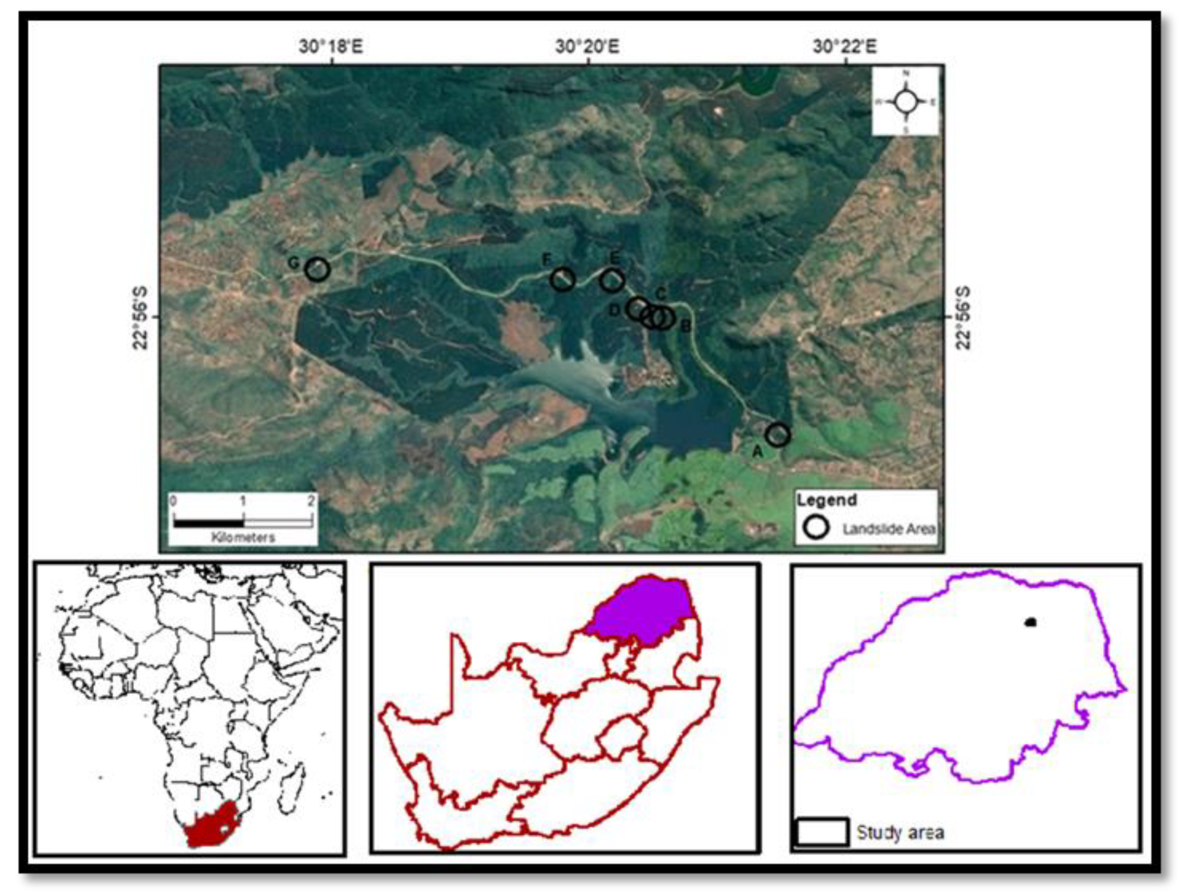
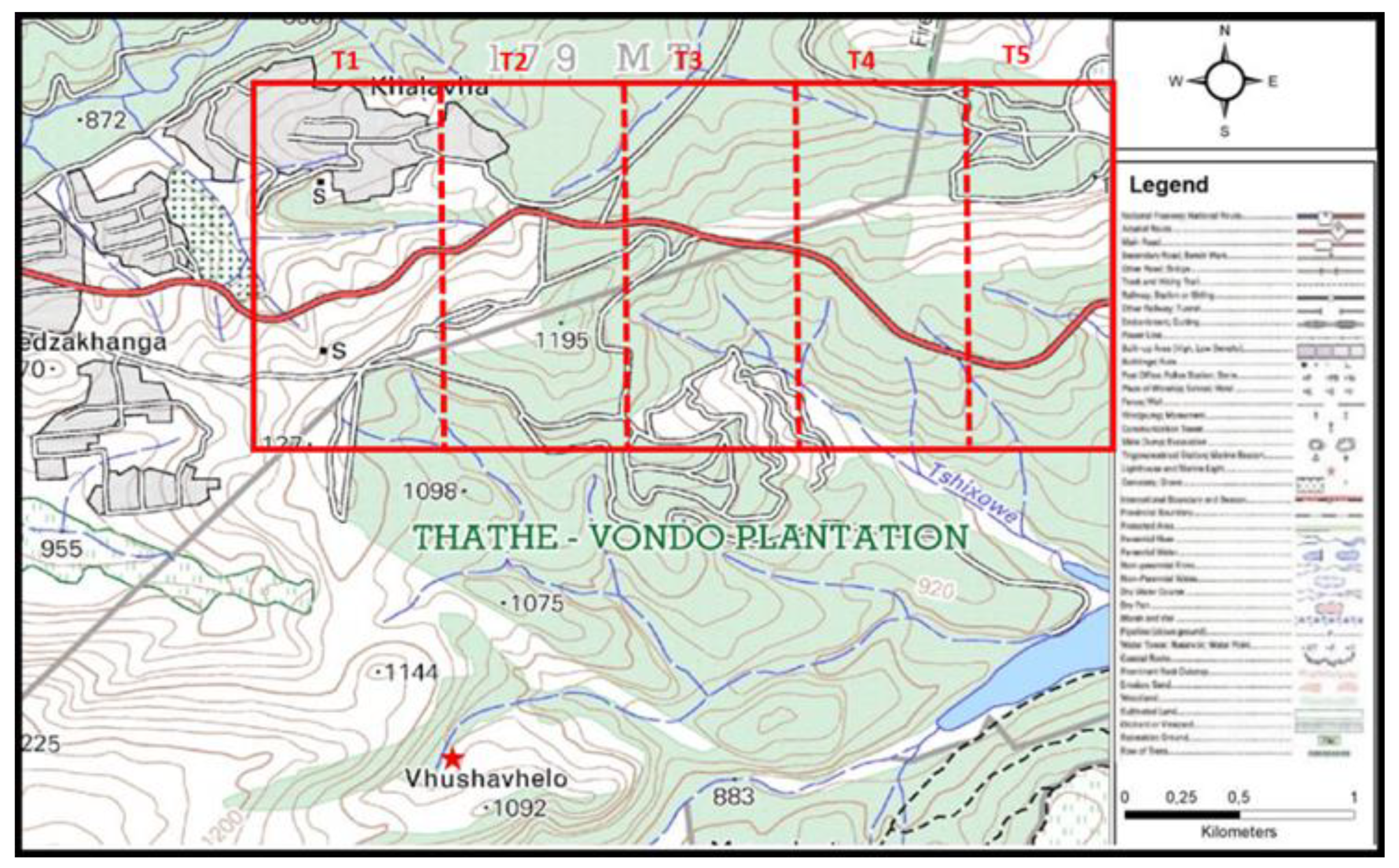
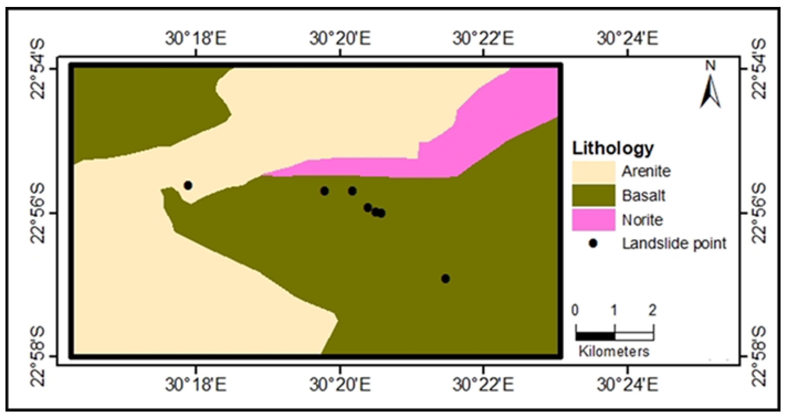
2. Location of the Study Area and Regional Geology Setting
3. Material and Method
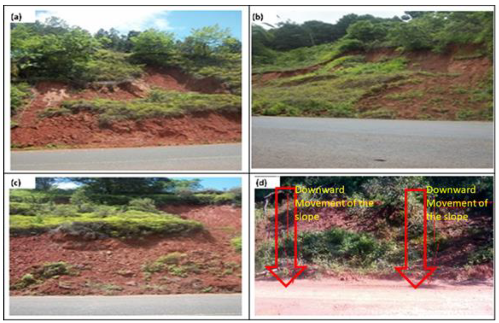
3.1. Visual Observations and Measurements
3.2. Sieve Analysis
3.3. Atterberg’s Limits
3.4. Influence of Rainfall Intensity on Slope Instability
3.5. Numerical Simulation
3.5.1. SLIDES (FEM) Model Procedures
3.5.2. FLACSlope (FDM) Model Procedures
4. Results and Discussion
4.1. Initial Results of the Field Observations
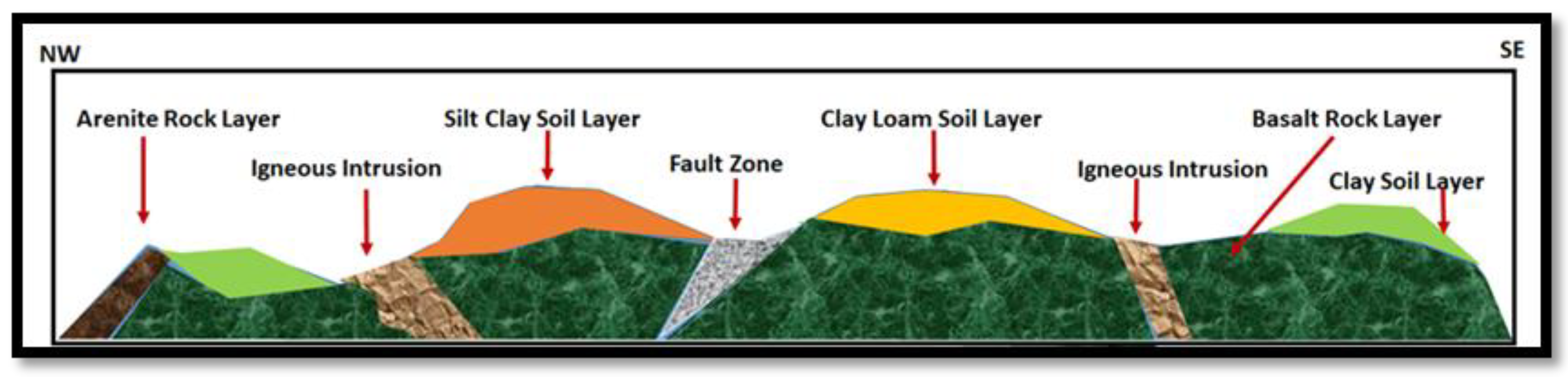
4.2. Geological Description of the Study Area
4.3. Mechanical Properties of the Soil
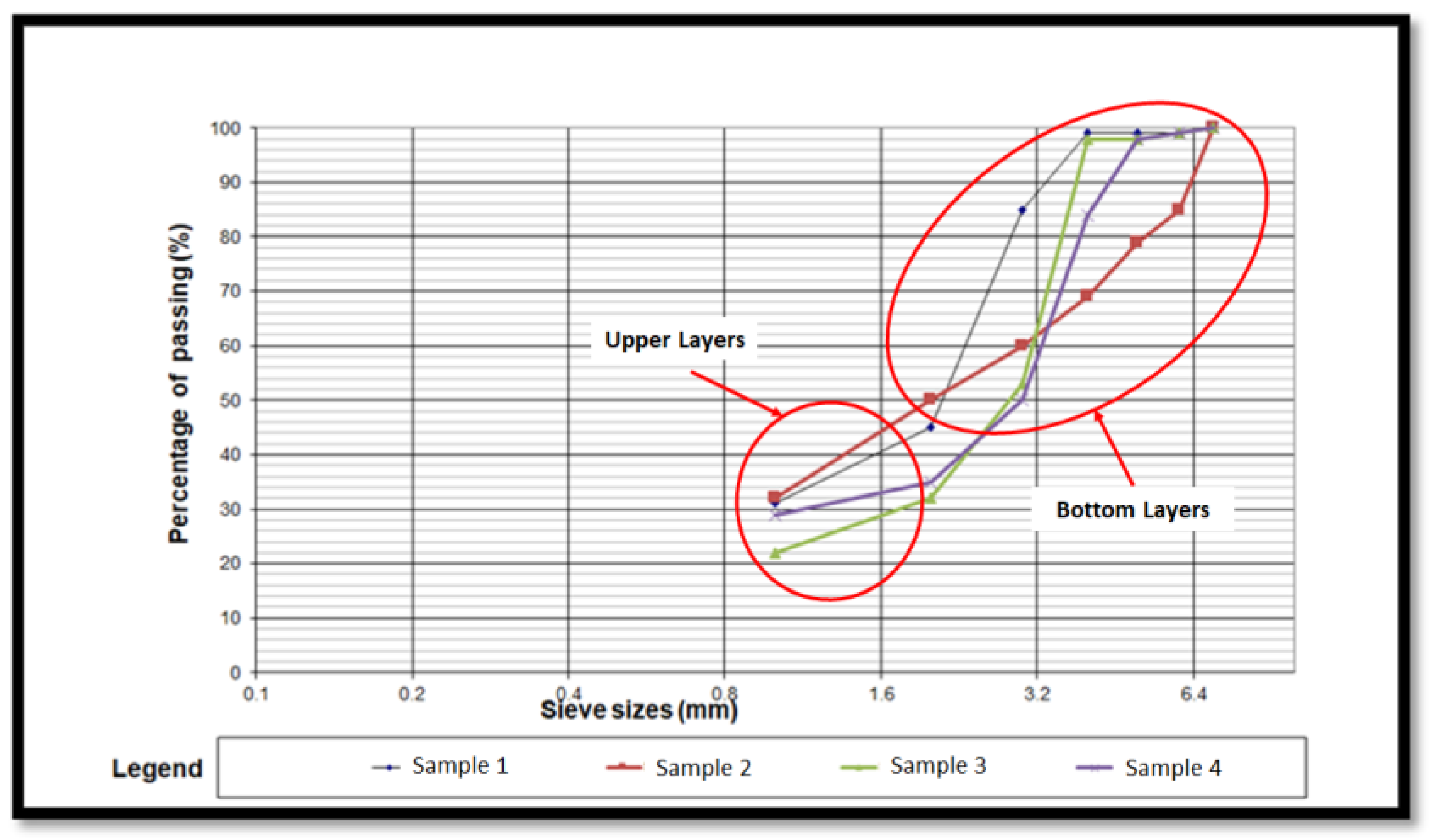
4.3.1. Particle Size Distribution
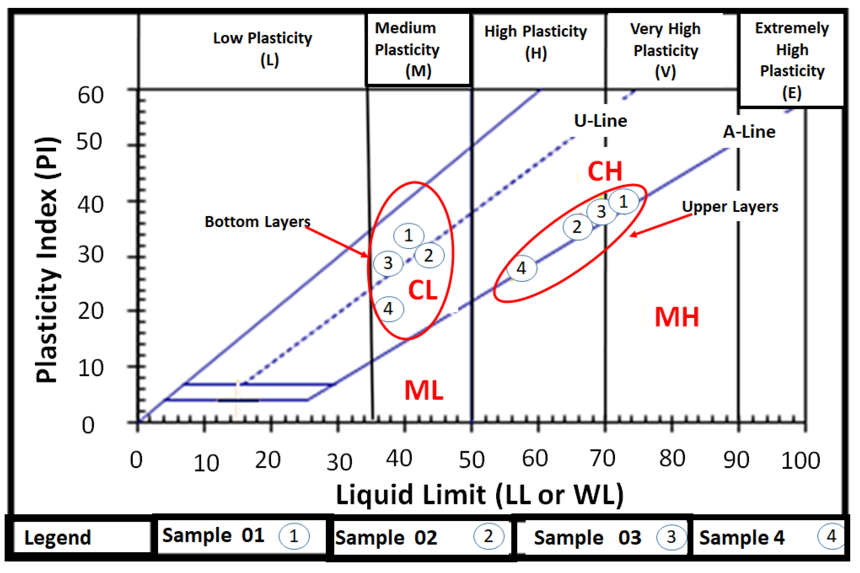
4.3.2. Atterberg’s Limits
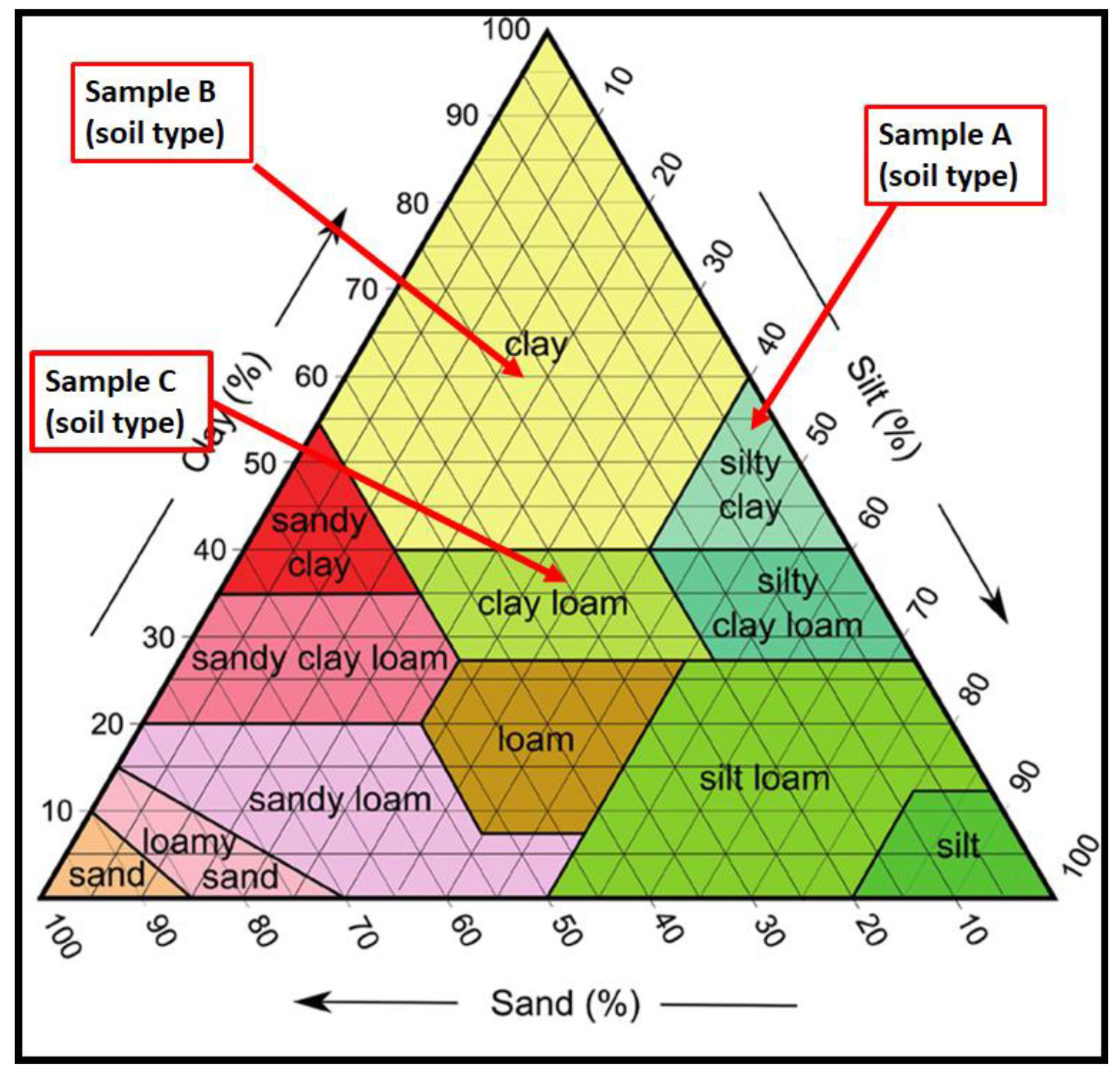
4.3.3. Soil Texture and Soil Types
4.3.4. Mechanical Properties of Soil
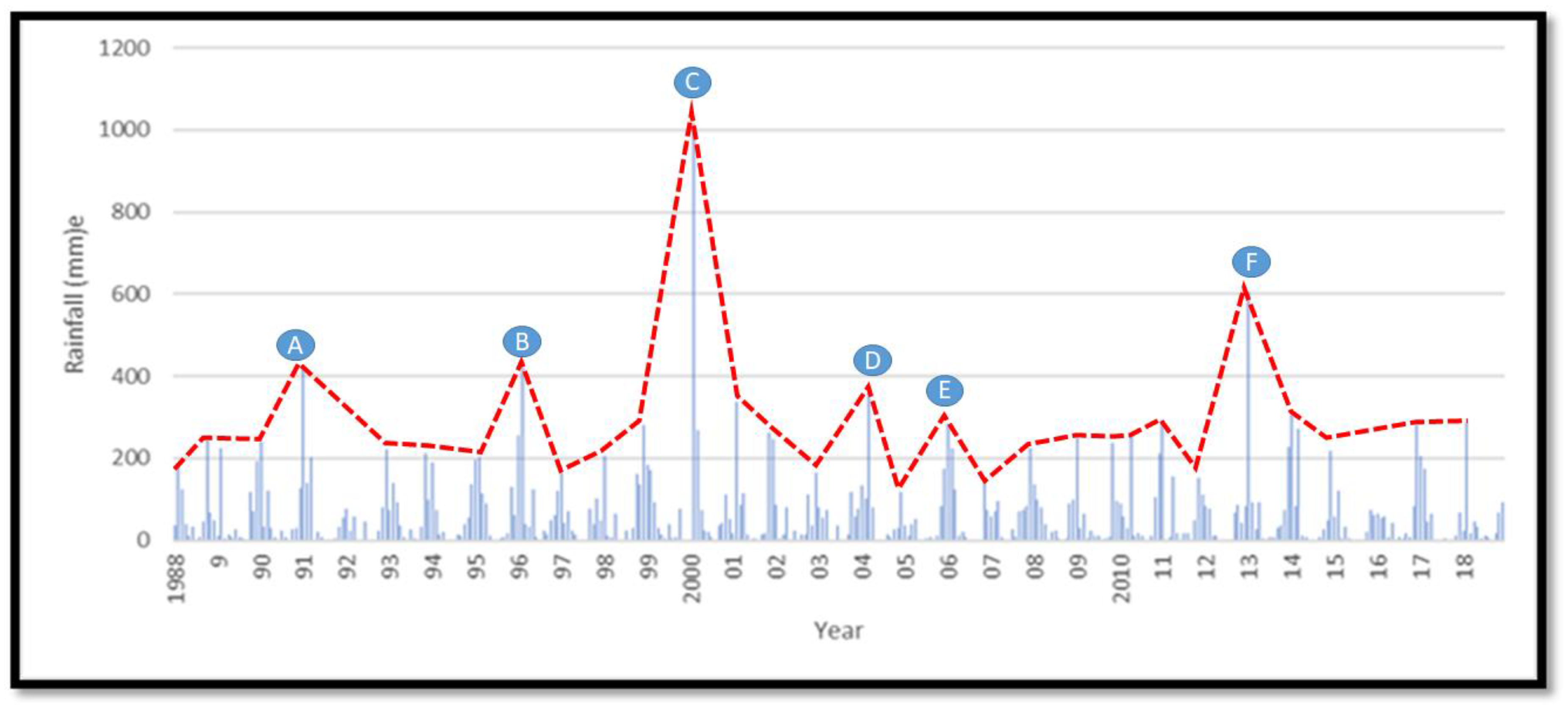
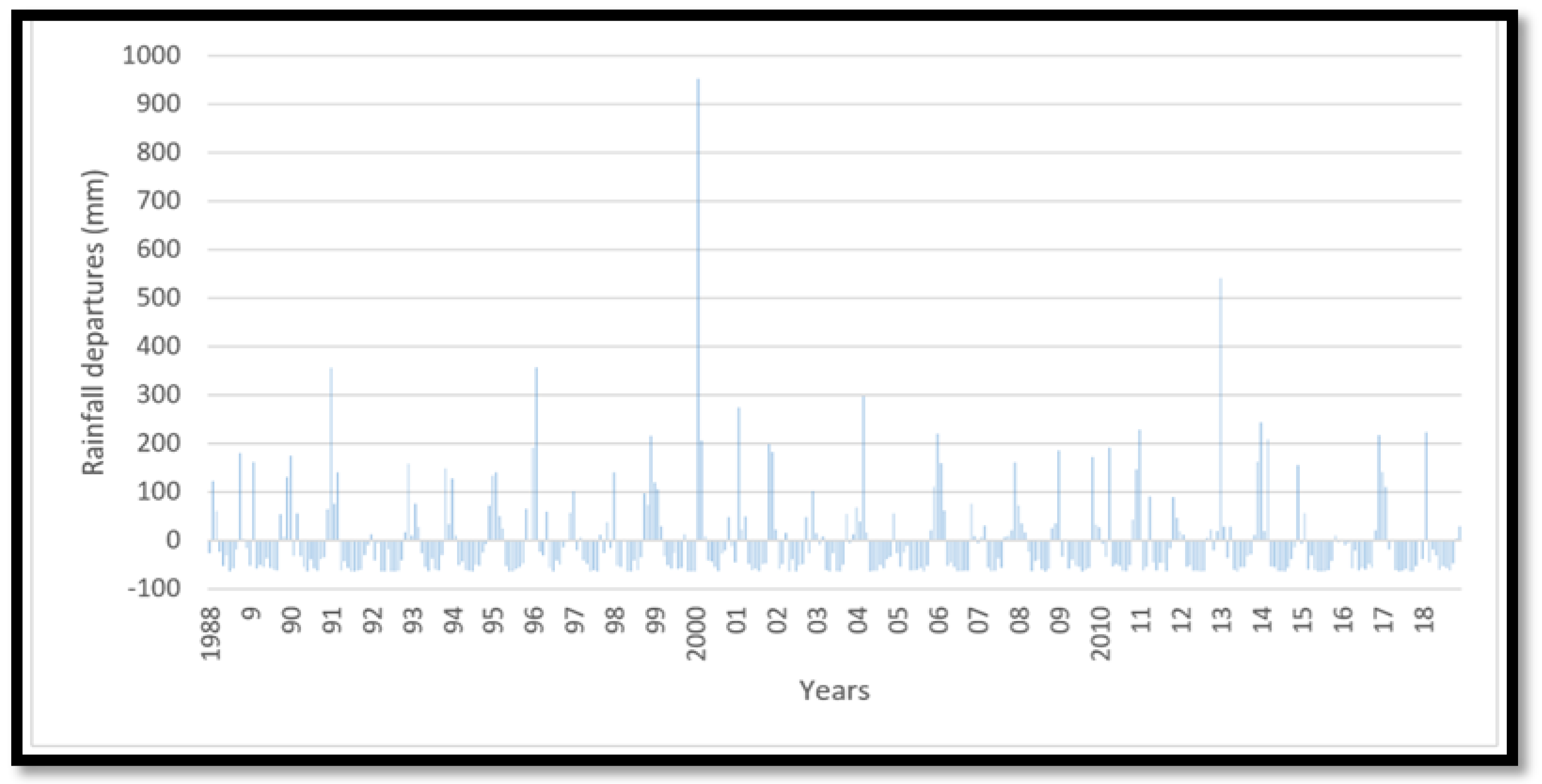
4.4. Rainfall in the Thulamela Municipality
4.5. Simulation of the Effects of Rainfall Intensity on Slope Stability
4.5.1. Simulation Case of a Clay Soil
Simulations of the FoS Using SLIDE Model under Sunny Conditions in Clay Soil Slope
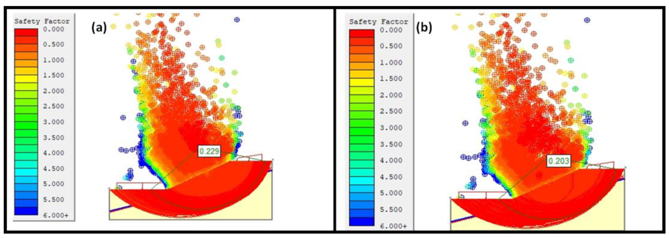
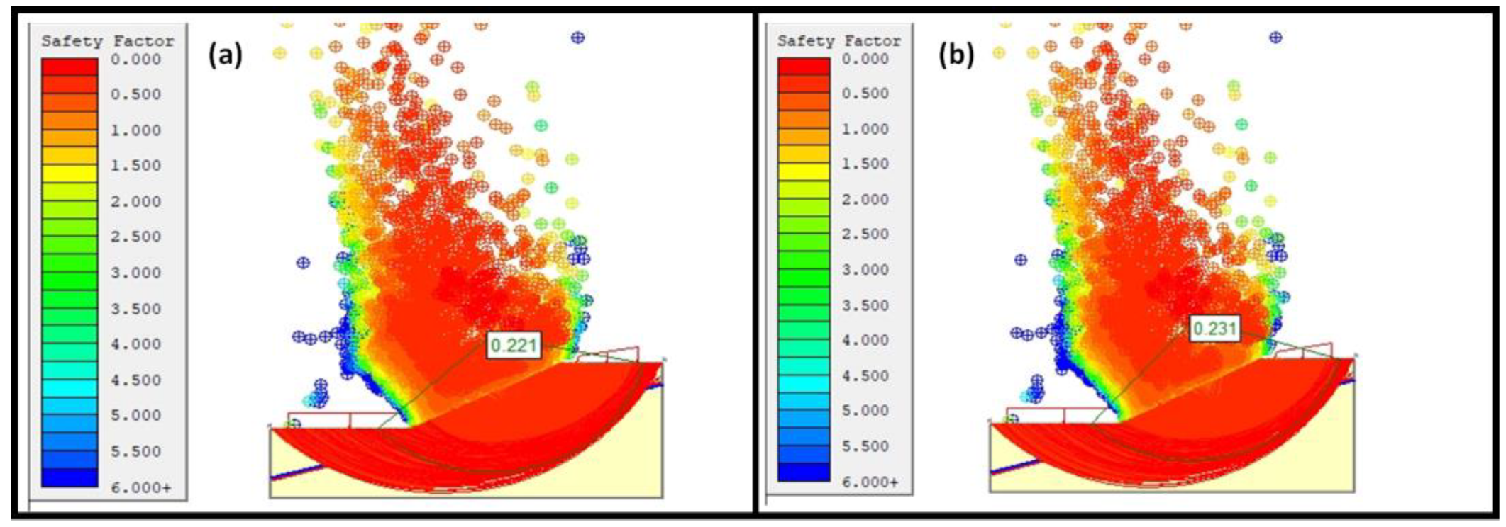
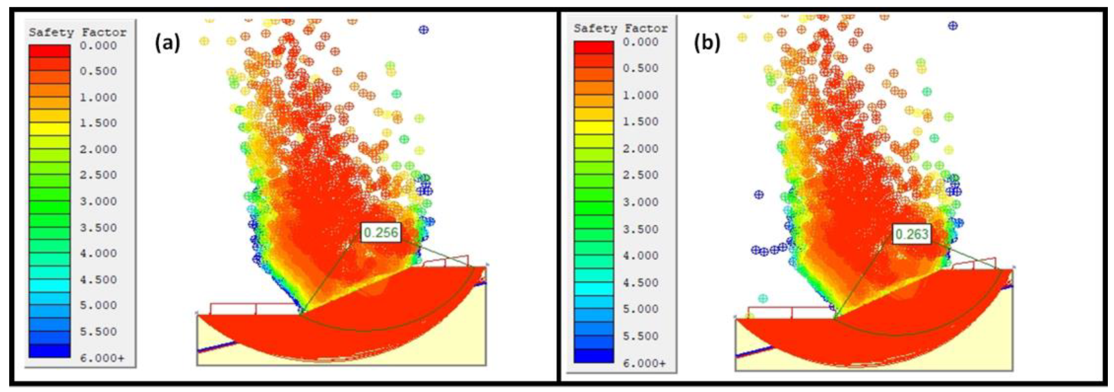
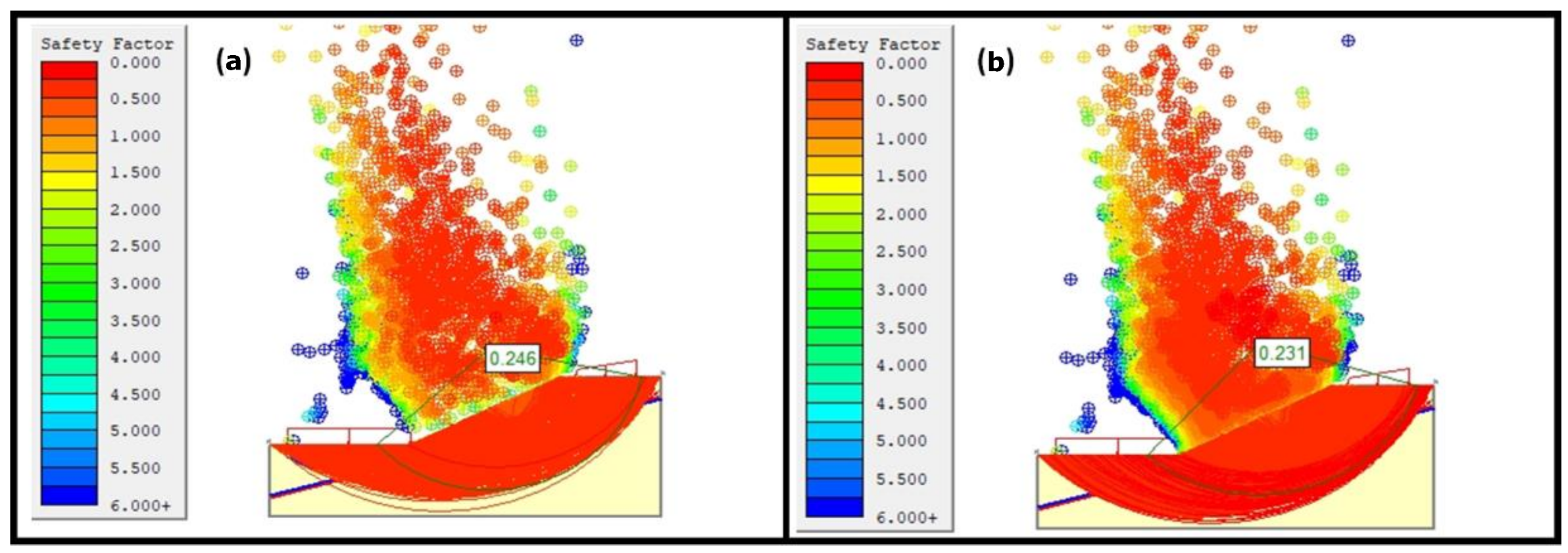
Simulations of the FoS Using SLIDE Model under Rainy Conditions in Clay Soil Slope
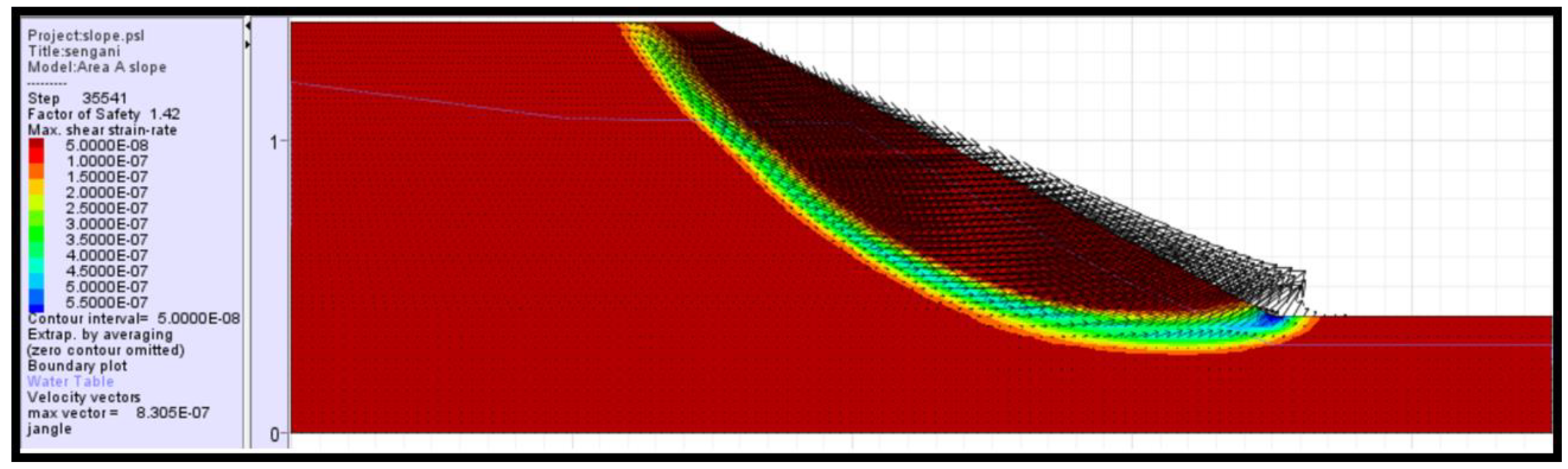
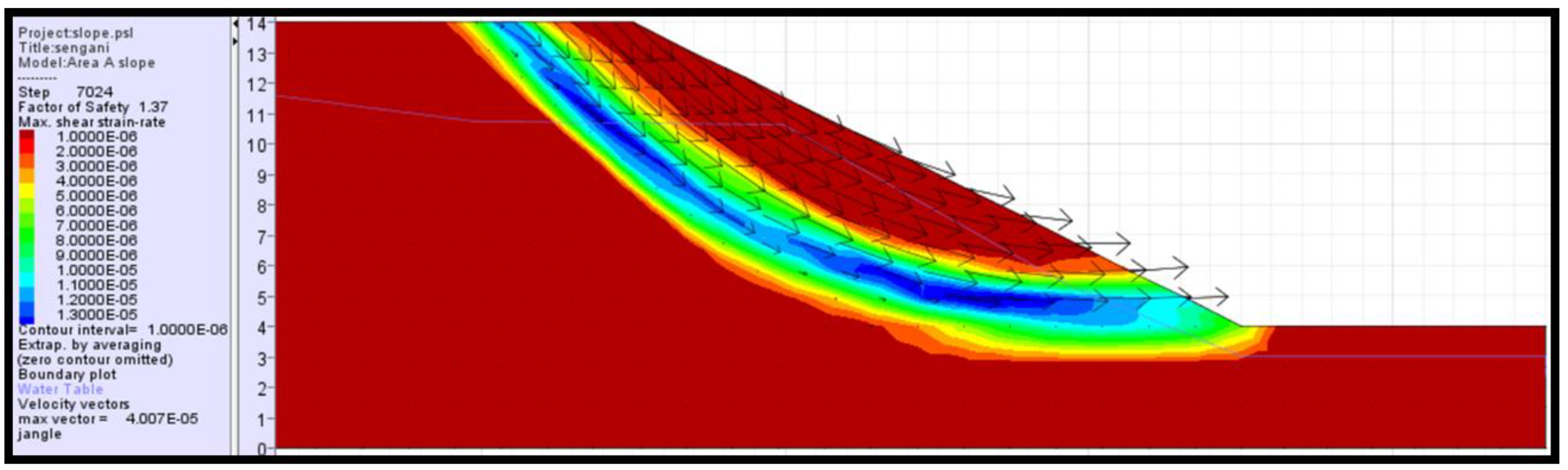
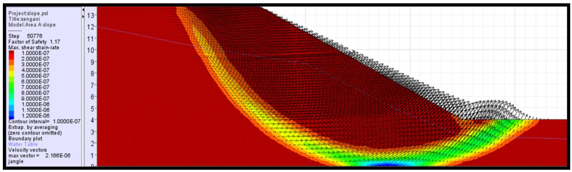
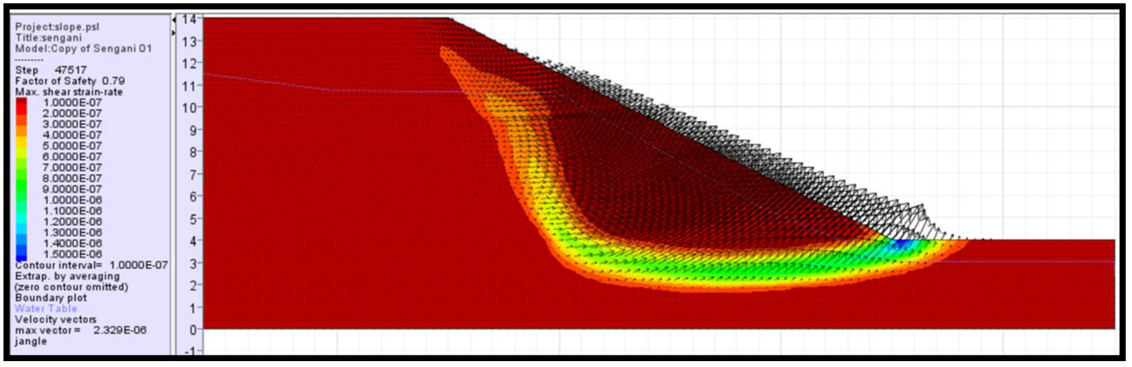
Simulations of the FoS Using FLACSlope (FDM) Model under Sunny to Rainy Conditions in Clay Soil Slope
4.5.2. Simulation Case of a Silt Clay Soil
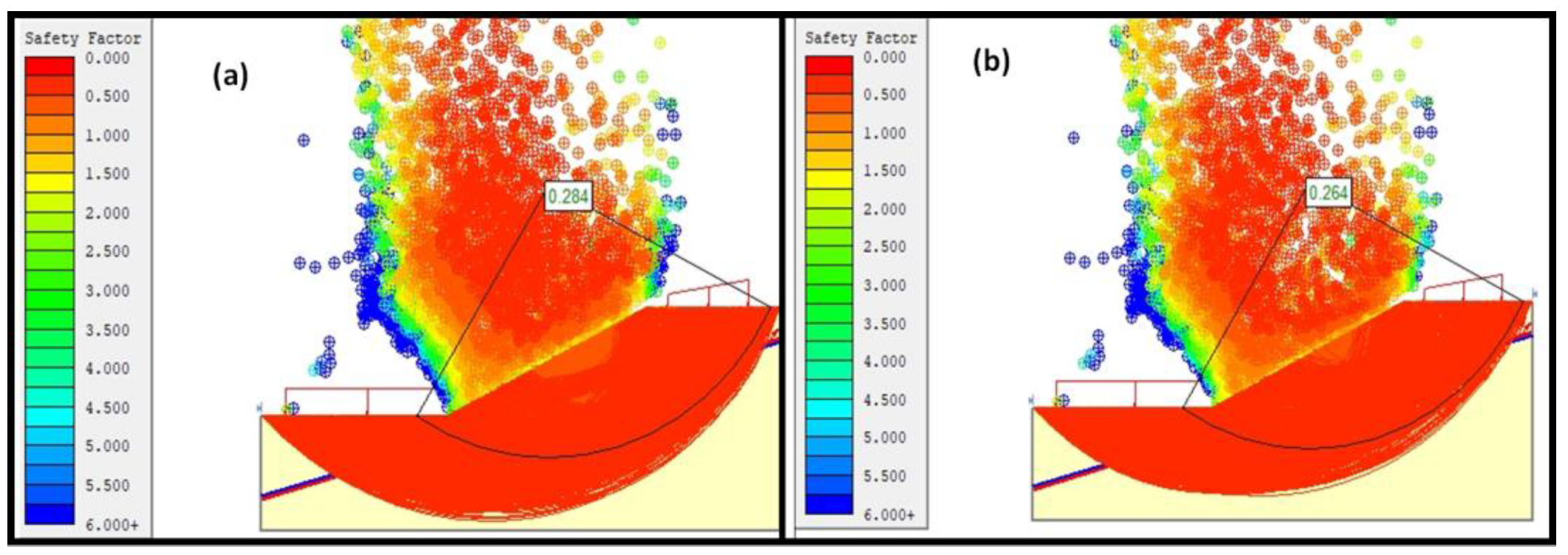
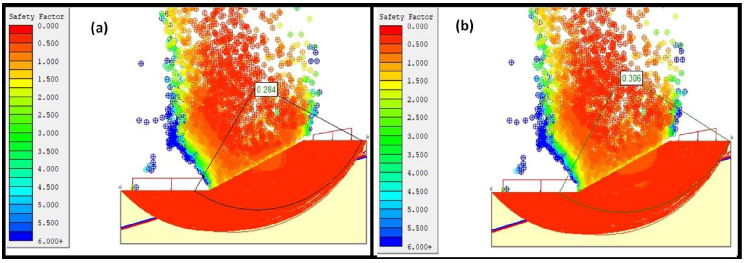
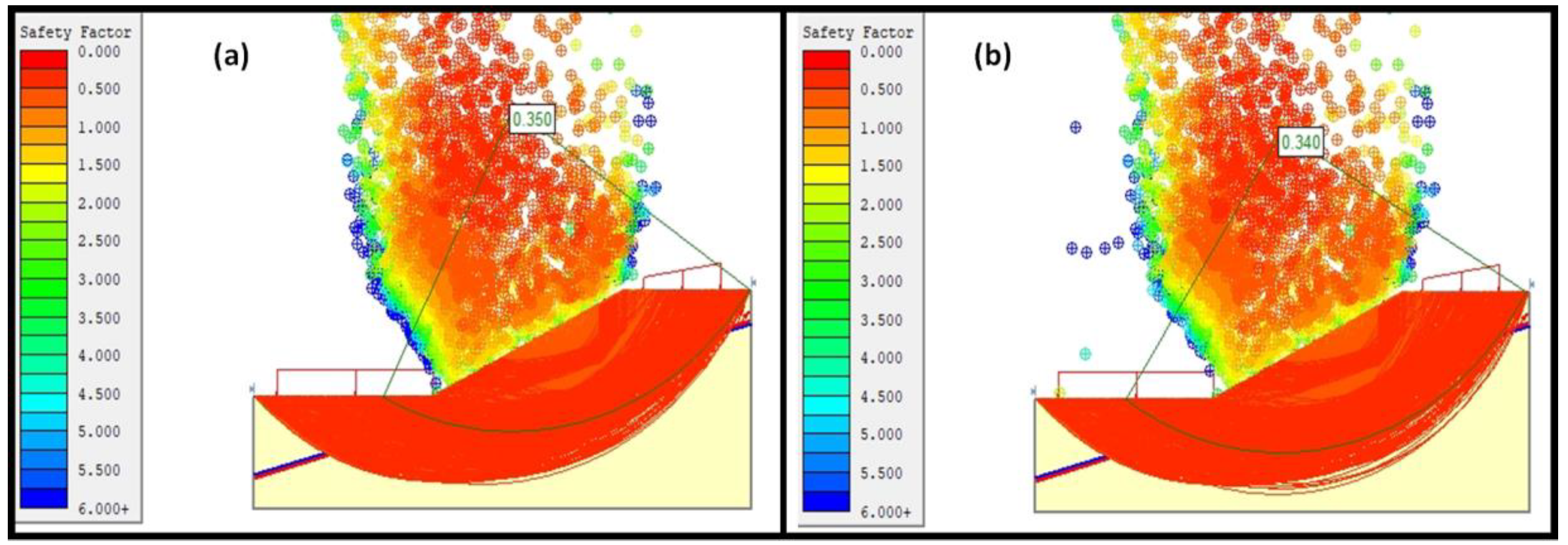
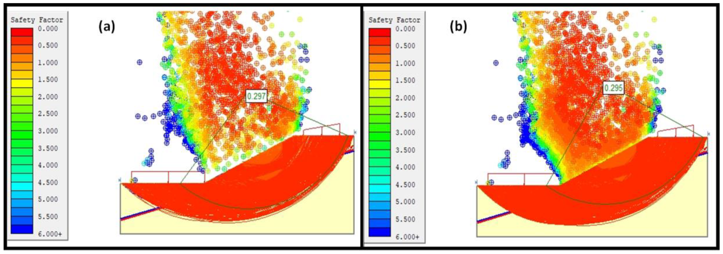
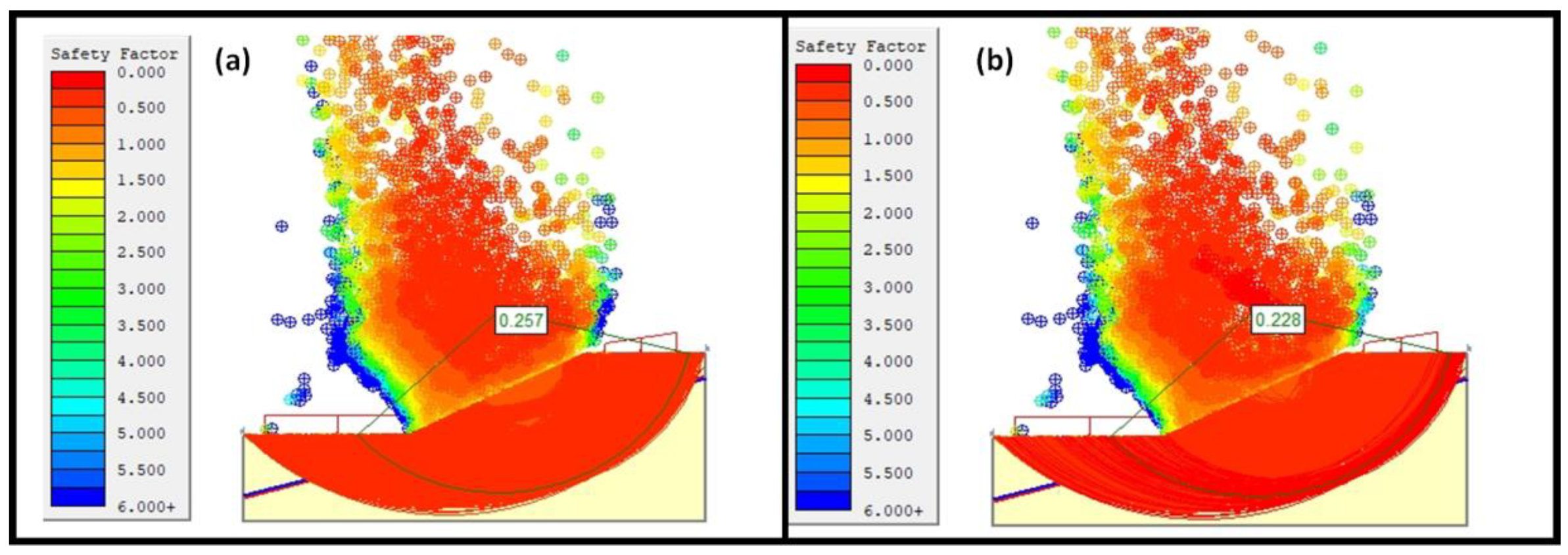
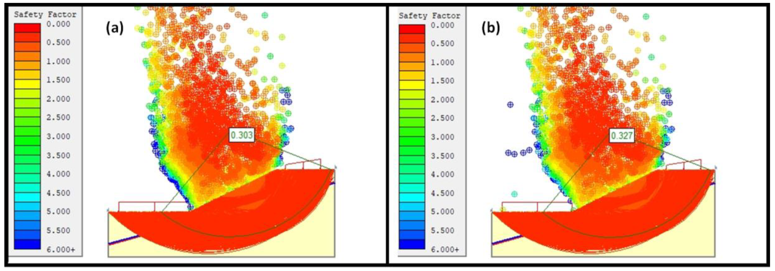
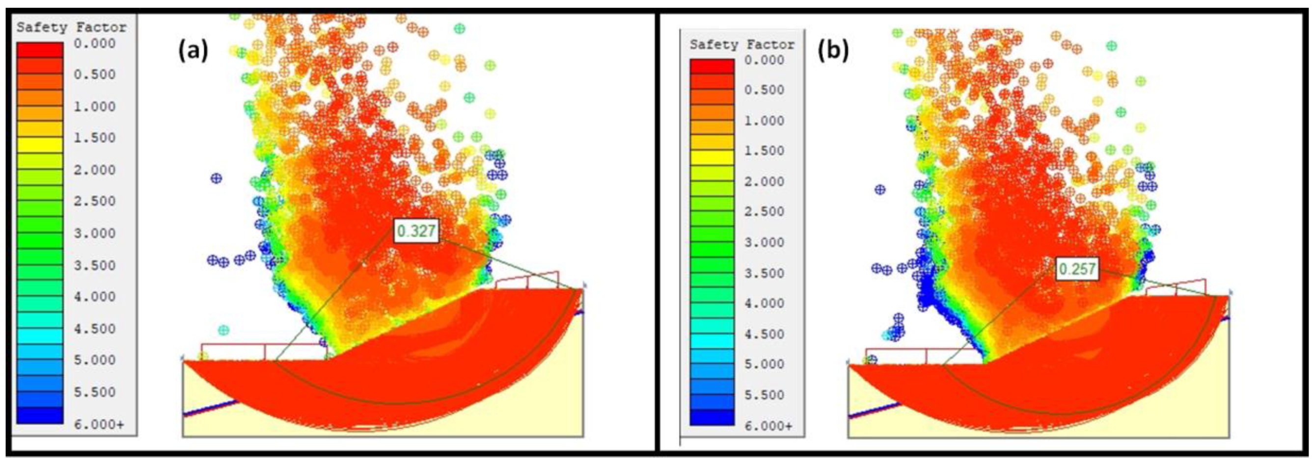
Simulations of the FoS Using SLIDE Model under Rainy Conditions in Silt Clay Soil Slope
Simulations of the FoS Using SLIDE Model under Rainy Conditions in Silt Clay Soil Slope
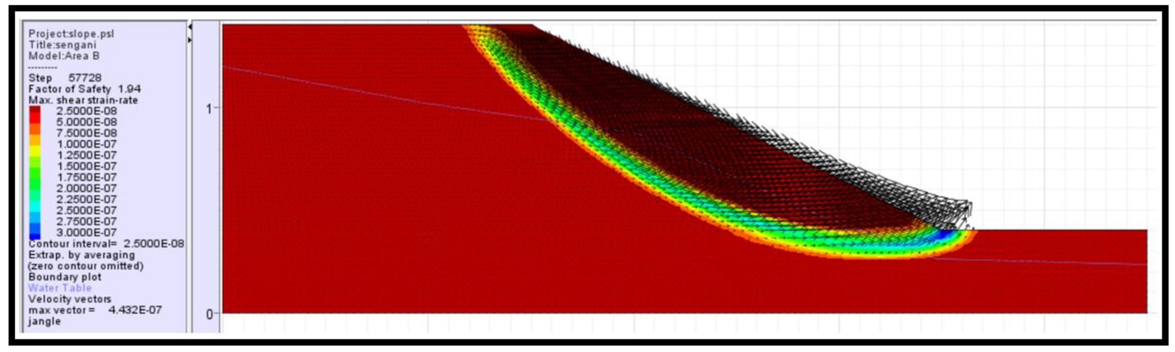
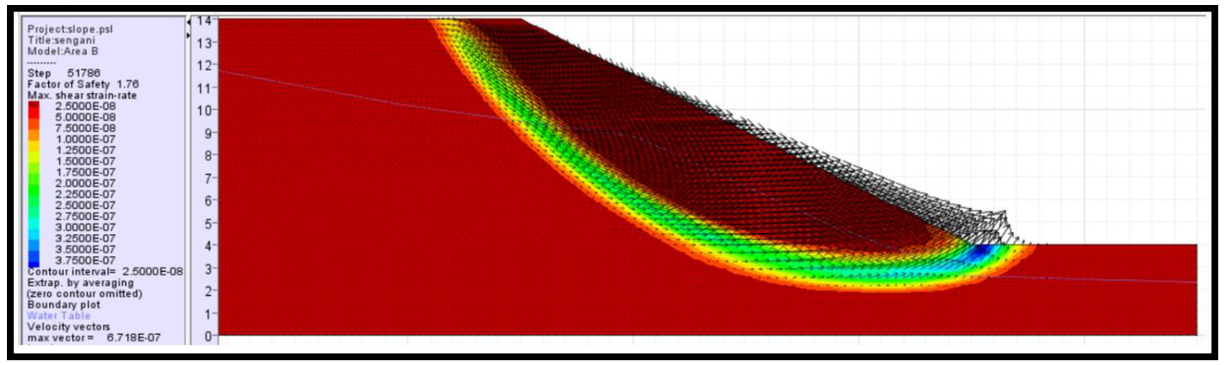
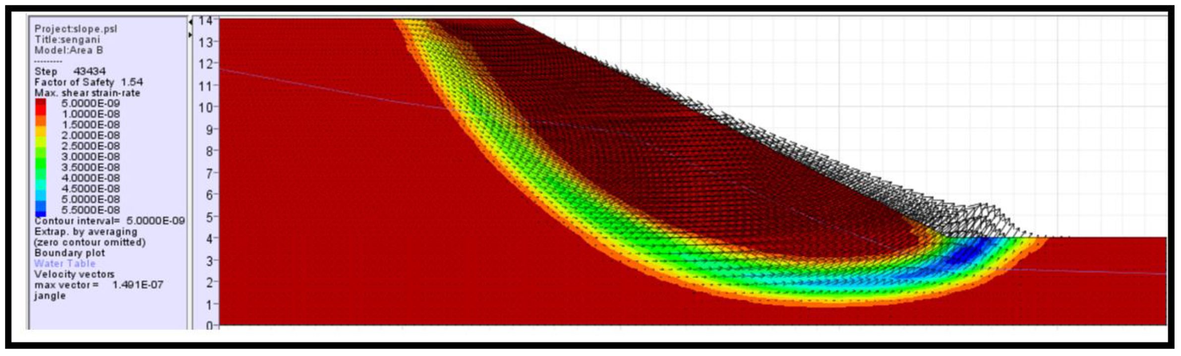
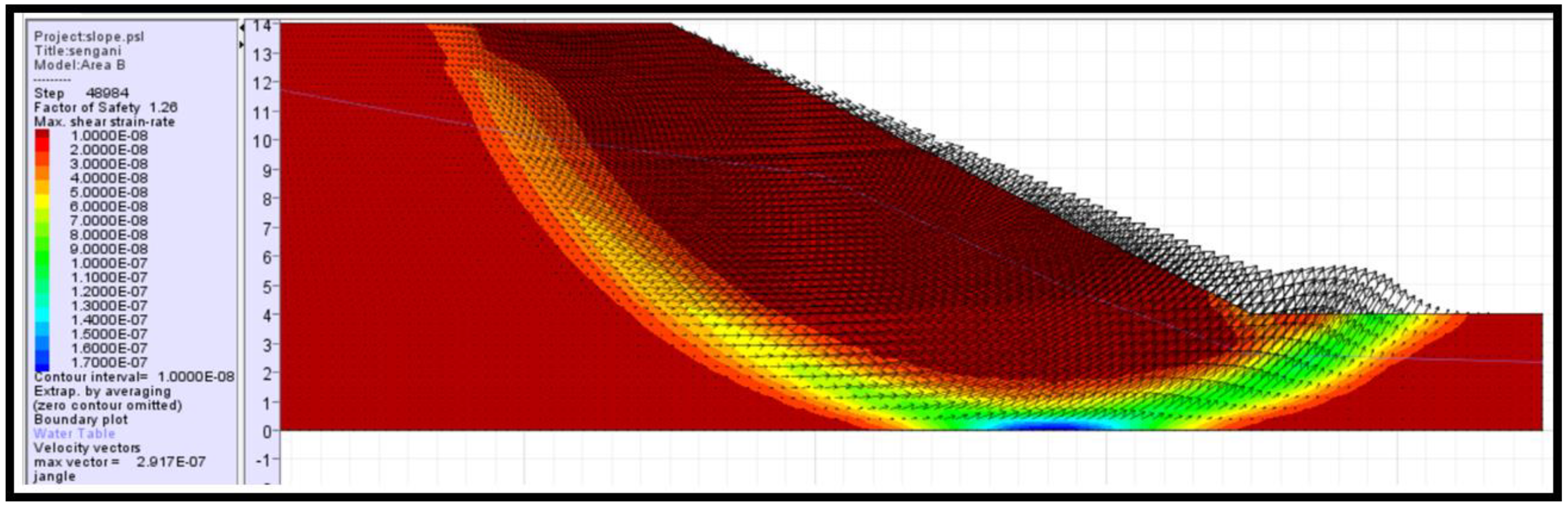
Simulations of the FoS Using FLACSlope (FDM) Model under Sunny to Rainy Conditions in Silt Clay Soil Slope
4.5.3. Simulation Case of a Clay Loam Soil
Simulations of the FoS Using SLIDE Model under Sunny Conditions in Clay Loam Soil Slope
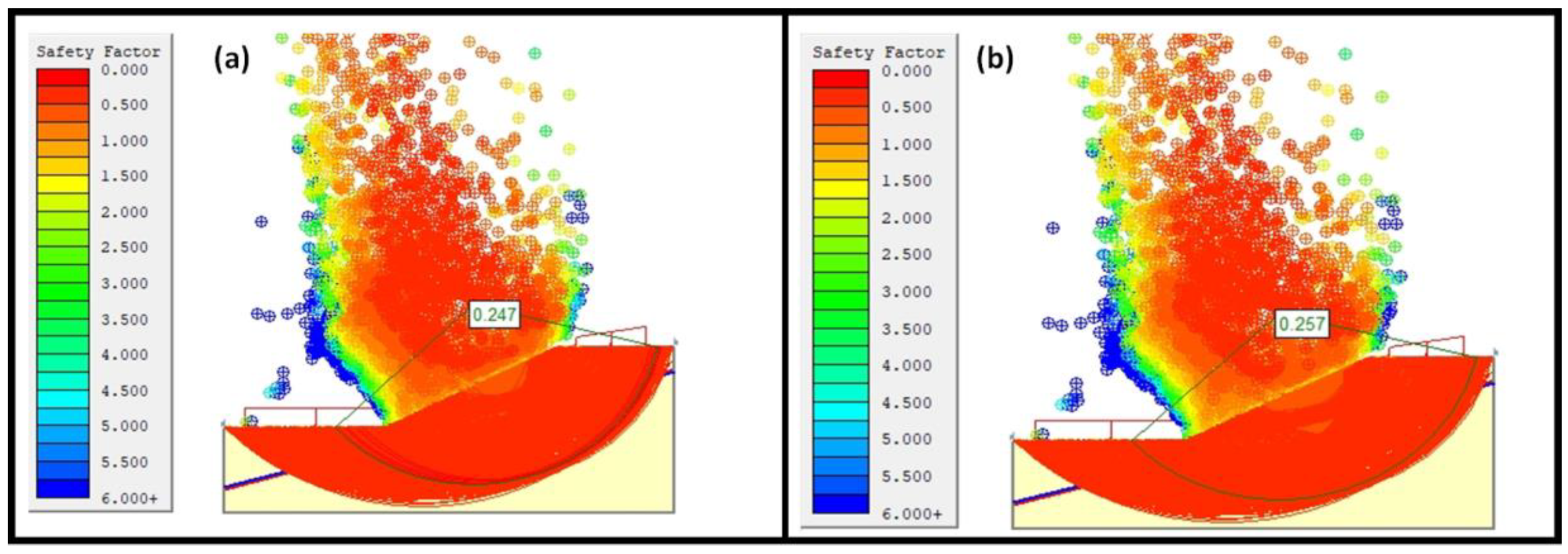
Simulations of the FoS Using SLIDE Model under Rainy Conditions in Clay Loam Soil Slope
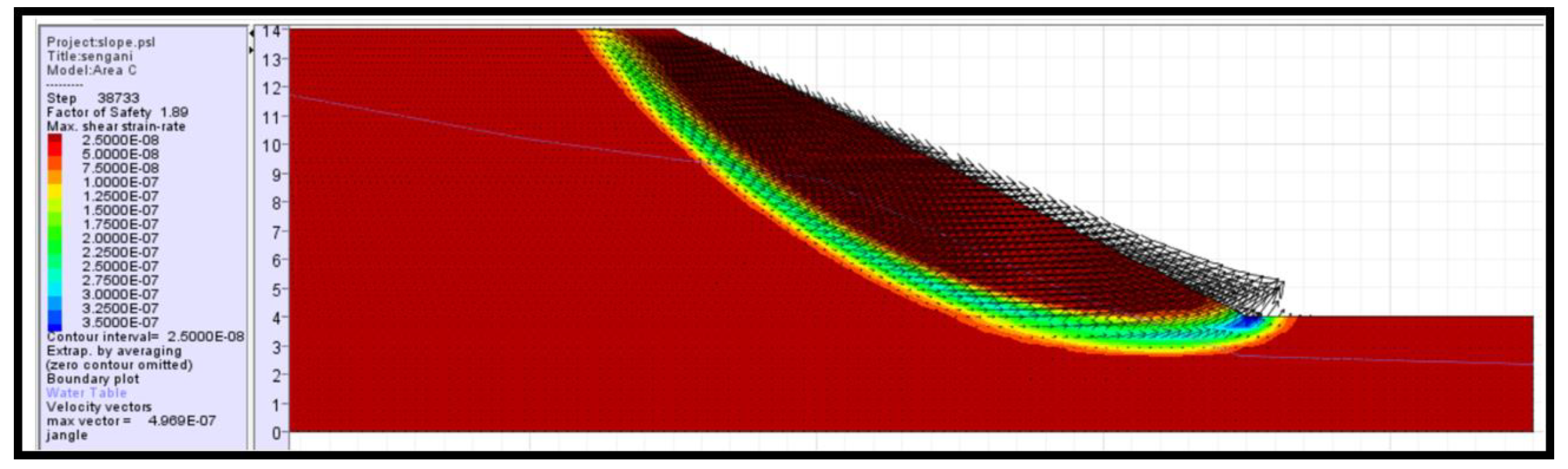
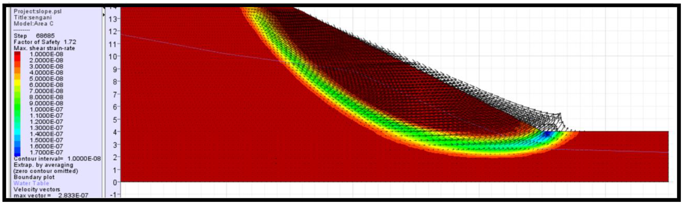
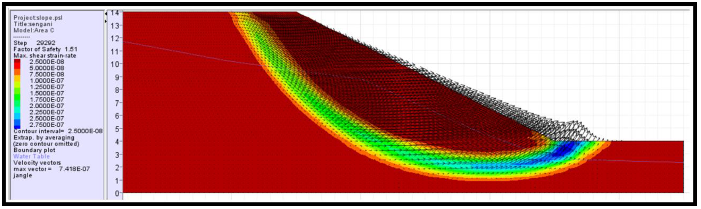
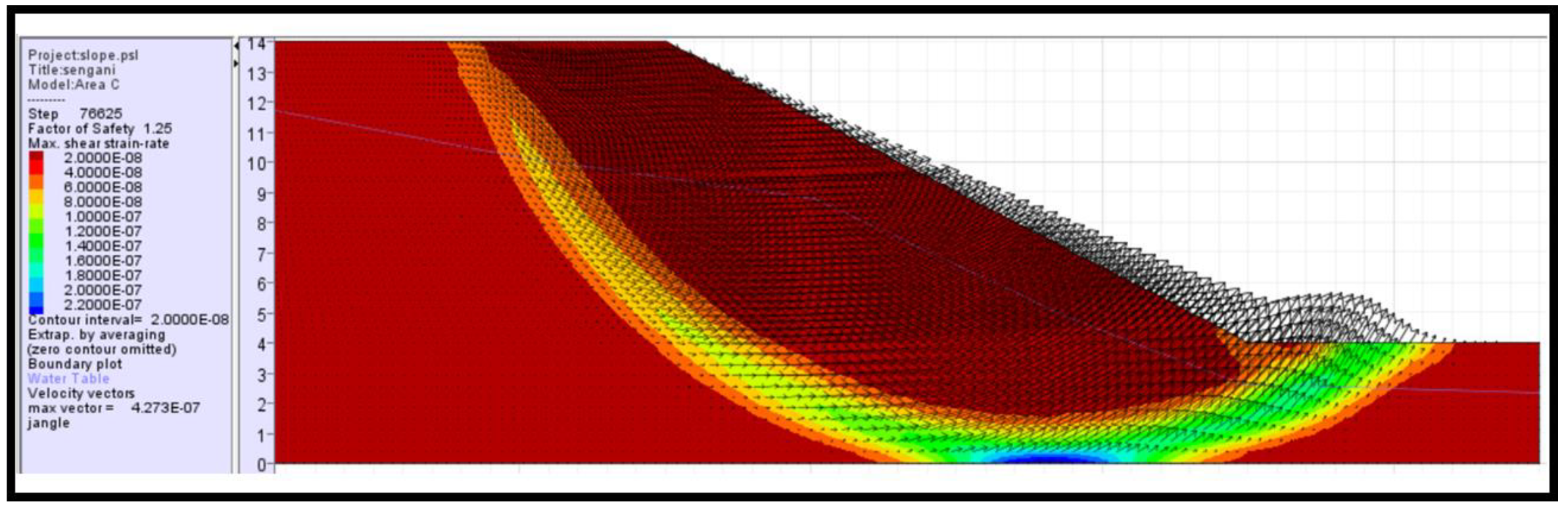
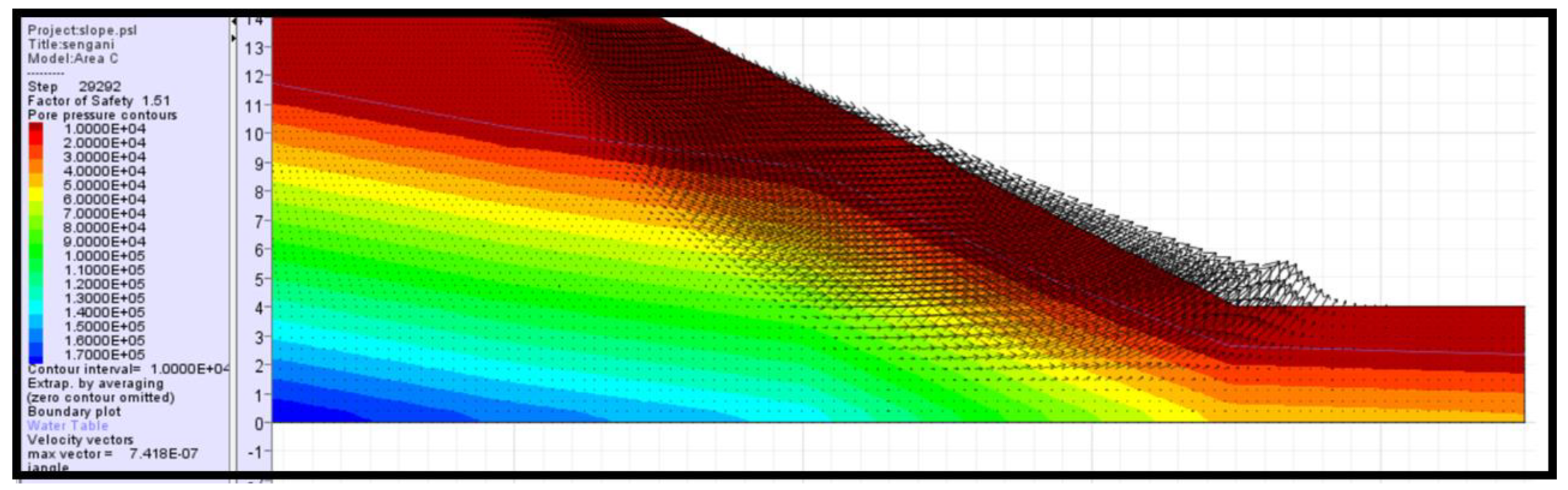
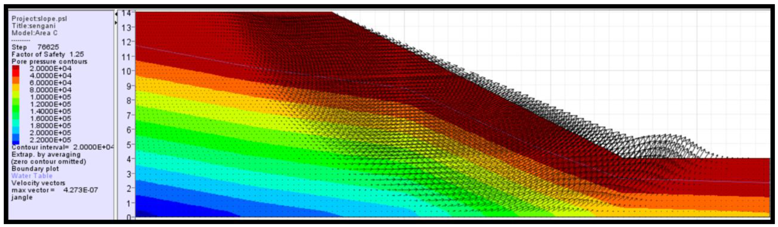
Simulations of the FoS Using FLACSlope (FDM) Model under Sunny to Rainy Conditions in Clay Loam Soil Slope
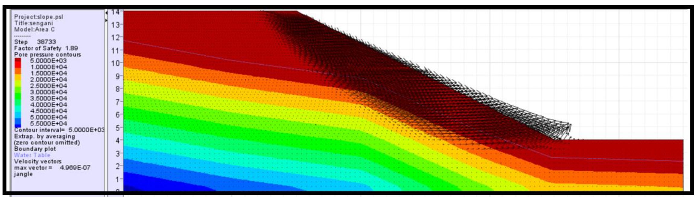
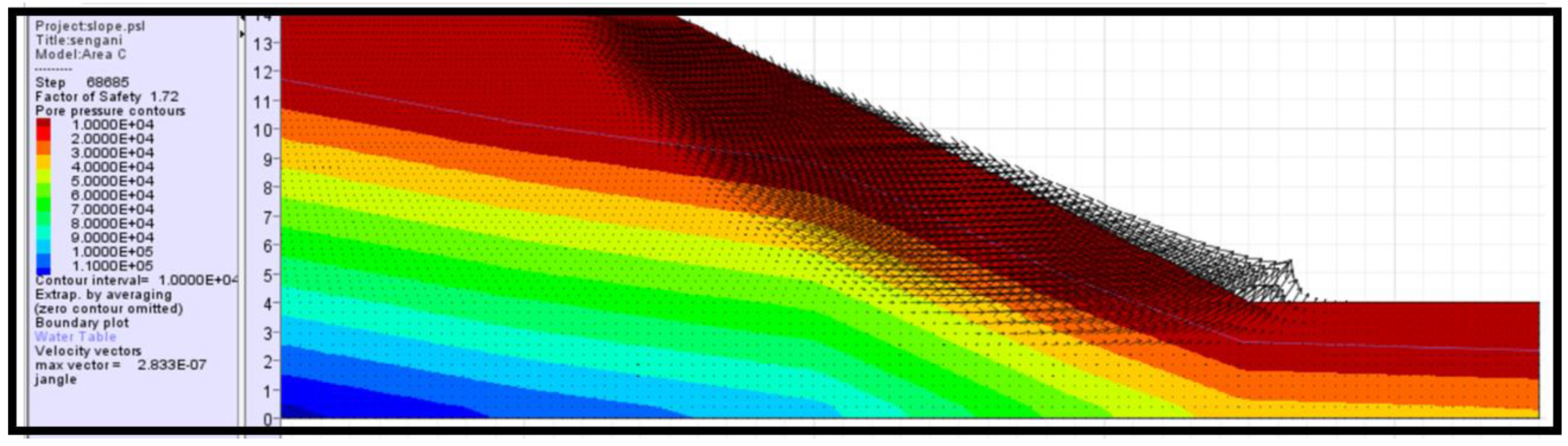
4.5.4. Simulation of Pore Pressure Variation Analysis in Case of Soil Slope
5. Significance of the Simulation Findings
6. Conclusions
Author Contributions
Funding
Acknowledgments
Conflicts of Interest
References
- Göktepe, I.; Keskin, F. A Comparison Study between Traditional and Finite Element Methods for Slope Stability Evaluations. J. Geol. Soc. India 2018, 91, 373–379. [Google Scholar] [CrossRef]
- Abbott, P.L. Natural Disasters; Mc-Graw-Hill: Boston, MA, USA, 2002. [Google Scholar]
- Bennett, M.R.; Doyle, P. Environmental Geology: Geology and the Human Environment; John Wiley & Sons: Chisester, UK, 1997. [Google Scholar]
- Guzzetti, F. Landslide fatalities and the evaluation of landslide risk in Italy. Eng. Geol. 2006, 58, 89–107. [Google Scholar] [CrossRef]
- Guzzetti, F.; Stark, C.P.; Salvati, P. Evaluation of flood and landslide risk to the opulation in Italy. Environ. Manag. 2005, 36, 15–36. [Google Scholar] [CrossRef] [PubMed]
- Lazzari, M.; Geraldi, E.; Lapenna, V.; Loperte, A. Natural hazards vs human impact: An integrated methodological approaching eomorphological risk assessing on Tursi historical site, southernItaly. Landslides 2006, 3, 275–287. [Google Scholar] [CrossRef]
- Lazzari, M. The Bosco Piccolo snow-melt triggered-landslide (southern Italy): A natural laboratory to apply integrated techniques to mapping, monitoring and damage assessment. In Proceedings of the Conference on Landslide Processes: From Geomorphologic Mapping to Dynamic Modelling, Strasbourg, France, 6–7 February 2009; pp. 163–168. [Google Scholar]
- Lazzari, M.; Piccarreta, M.; Capolongo, D. Landslide triggering and local rainfall thresholds in Bradanic Foredeep, Basilicata region (southern Italy). Landslide Science and Practice. Volume 2. Early warning, instrumentation and modeling. In Proceedings of the Second World Landslide Forum, Rome, Italy, 3–9 October 2011; Volume 2, pp. 671–678, ISBN 9783642314445. [Google Scholar]
- Lazzari, M.; Piccarreta, M.; Capolongo, D. Landslide triggering and local rainfall thresholds in bradanic foredeep, Basilicata Region (Southern Italy). In Landslide Science and Practice Volume 2: Early Warning, Instrumentationand Monitoring; Margottini, C., Canuti, P., Sassa, K., Eds.; Springer: Berlin/Heidelberg, Germany, 2013; pp. 671–677. [Google Scholar]
- Lazzari, M.; Gioia, D. Regional-scale landslide inventory, central-western sector of the Basilicata region (Southern Apennines, Italy). J. Maps 2015, 12, 852–859. [Google Scholar] [CrossRef]
- Lazzari, M.; Gioia, D.; Anzidei, B. Landslide inventory of the Basilicata region (Southern Italy). J. Maps 2018, 14, 348–356. [Google Scholar] [CrossRef] [Green Version]
- Bogaard, T.A.; Greco, R. Landslide hydrology: From hydrology to pore pressure. WIREs Water 2016, 3, 439–459. [Google Scholar] [CrossRef]
- Sengani, F.; Mulenga, F. Application of Limit Equilibrium Analysis and Numerical Modeling in a Case of Slope Instability. Sustainability 2020, 12, 8870. [Google Scholar] [CrossRef]
- Sengani, F.; Zvarivadza, T. Evaluation of factors influencing slope instability: Case study of the R523 Road between Thathe Vondo and khalavha area in South Africa. In Symposium of Environmental Issues and Waste Management in Energy and Mineral Production; Springer: Berlin/Heidelberg, Germany, 2019; pp. 81–89. [Google Scholar]
- Mutanamba, M. Analyze the Stability of Cut Slopes along the R523 Road between Thathe Vondo and Khalavha Area and to Find the Most Appropriate Stabilization Methods to Prevent Future Slope Failure along the Road R523. Master’s Thesis, University of Venda, Venda, South Africa, 2013. [Google Scholar]
- Chen, Y.C.; Chang, K.T.; Wang, S.F.; Huang, J.C.; Yu, C.K.; Tu, J.Y.; Chu, H.J.; Liu, C.C. Controls of preferential orientation of earthquake- and rainfall-triggered landslides in Taiwan’s orogenic mountain belt. Earth Surf. Process. Landf. 2019, 44, 1661–1674. [Google Scholar] [CrossRef]
- Bucci, F.; Santangelo, M.; Cardinali, M.; Fiorucci, F.; Guzzetti, F. Landslide distribution and size in response to Quaternary fault activity: The Peloritani Range, NE Sicily, Italy. Earth Surf. Process. Landf. 2016, 41, 711–720. [Google Scholar] [CrossRef] [Green Version]
- Kluger, M.O.; Moon, V.G.; Kreiter, S.; Lowe, D.J.; Churchman, G.J.; Hepp, D.A.; Mörz, T. A new attraction-detachment model for explaining flow sliding in clay-rich tephras. Geology 2017, 45, 131–134. [Google Scholar] [CrossRef] [Green Version]
- Imaizumi, F.; Sidle, R.C.; Togari-Ohta, A.; Shimamura, M. Temporal and spatial variation of infilling processes in a landslide scar in a steep mountainous region, Japan. Earth Surf. Process. Landf. 2015, 40, 642–653. [Google Scholar] [CrossRef]
- Goswami, R.; Mitchell, N.C.; Brocklehurst, S.H. Distribution and causes of landslides in the eastern Peloritani of NE Sicily and western Aspromonte of SW Calabria, Italy. Geomorphology 2011, 132, 111–122. [Google Scholar] [CrossRef]
- Guo, C.; Montgomery, M.C.; Zhang, Y.; Wang, K.; Yanga, Z. Quantitative assessment of landslide susceptibility along the Xianshuihe fault zone, Tibetan Plateau, China. Geomorphology 2015, 248, 93–110. [Google Scholar] [CrossRef]
- Thulamela Municipality. Background of Thulamela Municipality. Thulamela Municipality Limpopo Province. 2019. Available online: http://www.thulamela.gov.za/index.php?page=background (accessed on 28 September 2020).
- Barker, O.B. A contribution to the geology of the Soutpansberg Group, Waterberg Supergroup, Northern Transvaal. Ph.D. Thesis, University of the Witwatersrand, Johannesburg, South Africa, 1979. [Google Scholar]
- Barker, O.B.; Brandl, G.; Callaghan, C.C.; Erikson, P.G.; van der Neut, M. The Soutpansberg and Waterburg Groups and the Blouberg formation. In The Geology of South Africa; Anhaeusser, M.R., Thomas, C.R., Johnson, R.J., Eds.; Council for Geosciences, Geological Society of South Africa: Pretoria, South Africa, 2006; pp. 301–324. [Google Scholar]
- Brandl, G. The Geology of the Messina Area. Explain. Sheet 2230 (Messina); Report Number 35; Geology Survey of South Africa: Pretoria, South Africa, 1981. [Google Scholar]
- Brandl, G. The Geology of Pieterburg Area. Explain. Sheet 2230 (Pietersburg); Report Number 43; Geology Survey of South Africa: Pretoria, South Africa, 1986. [Google Scholar]
- Wyllie, D.C.; Mah, C.W. Rock Slope Engineering, Civil and Mining, 4th ed.; Taylor & Francis: London, UK; New York, NY, USA, 2004. [Google Scholar]
- Das, B.M. Principles of Geotechnical Engineering, 7th ed.; Cengage Learning: Stamford, CT, USA, 2010. [Google Scholar]
- Budetta, P. Assessment of rockfall risk along roads. Nat. Hazards Earth Syst. Sci. 2004, 4, 71–81. [Google Scholar] [CrossRef] [Green Version]
- Bishop, A.W. The use of the slip circle in the stability analysis of slopes. Geotechnique 1955, 5, 7–17. [Google Scholar] [CrossRef]
- Janbu, N. Slope Stability Computations. Soil Mechanics and Foundation Engineering Report; Technical University of Norway: Trondheim, Norway, 1968. [Google Scholar]
- Spencer, E. A method of analysis of the stability of embankments assuming parallel interslice forces. Geotechnique 1967, 17, 11–26. [Google Scholar] [CrossRef]
- U.S. Army Corps of Engineers. Engineering and Design—Stability of Earth and Rockfill Dams; Engineer Manual EM 1110-2-1902; Department of the Army, Corps of Engineers: Washington, DC, USA, 1970.
- Lowe, J.; Karafiath, L. Stability of earth dams upon drawdown. In Proceedings of the 1st Pan-American Conference on Soil Mechanics and Foundation Engineering; Mexico Society for Soil Mechanics: Mexico City, Mexico, 1960; Volume 2, pp. 537–552. [Google Scholar]
- Morgenstern, N.R.; Price, V.E. The analysis of the stability of general slip surfaces. Geotechnique 1965, 15, 79–93. [Google Scholar] [CrossRef]
- Duncan, J.M. State of the art: Limit equilibrium and finite-element analysis of slopes. J. Geotech. Eng. (ASCE) 1996, 122, 577–596. [Google Scholar] [CrossRef]
- Fang, H.; Daniels, J.L. Introductory Geotechnical Engineering: An Environmental Perspective; Tailor and Francis: London, UK; New York, NY, USA, 2006. [Google Scholar]
- Blakemore, L.C.; Swindale, L.D. The Chemistry and Clay Mineralogy of a Soil Sample from Antarctica. Natrue (Land.) 1958, 182, 47–48. [Google Scholar] [CrossRef]
- Kelly, W.C.; Zumberge, J.H. Weathering of a Quartz Diorite at Marble Point, McMurdo Sound, Antarctica. J. Geol. 1961, 69, 433–446. [Google Scholar] [CrossRef]
- Al-Karni, A.A. Effect of Pore Water Pressure on Stress- Strain Characteristics of Dense Sand, Soil and Rock Behavior and Modeling. GSP 2006, 150, 35–41. [Google Scholar]
- Aleotti, P. A warning system for rainfall-induced shallow failures. Eng. Geol. 2004, 73, 247–265. [Google Scholar] [CrossRef]
- Brunetti, M.T.; Peruccacci, S.; Rossi, M.; Luciano, S.; Valigi, D.; Guzzetti, F. Rainfall thresholds for the possible occurrence of landslides in Italy. Nat. Hazards Earth Syst. Sci. 2010, 10, 447–458. [Google Scholar] [CrossRef]
- Caine, N. The rainfall intensity-duration control of shallow landslides and debris flows. Geogr. Ann. 1980, 62A, 23–27. [Google Scholar]
- Cannon, S.H.; Gartner, J.E.; Wilson, R.C.; Bowers, J.C.; Laber, J.L. Storm rainfall conditions for floods and debris flows from recently areas in Southwestern Colorado and southern California. Geomorphology 2008, 96, 250–269. [Google Scholar] [CrossRef]
- Cevasco, A.; Sacchini, A.; Robbiano, A.; Vincenzi, E. Evaluation of rainfall thresholds for triggering shallow landslides on the Genoa municipality area (Italy): The case study of the Bisagno Valley. Italian J. Eng. Geol. Environ 2010, 1, 35–50. [Google Scholar]
- Corominas, J.; Moya, J.; Hurlimann, M. Landslide rainfall triggers in the Spanish Eastern Pyrenees. Mediterranean Storms. In Proceedings of the 4th EGS Plinius conference, Mallorca, Italy, 14–16 October 2002. [Google Scholar]
- Crosta, G.B.; Agliardi, F. Failure forecast for large rock slides by surface displacement measurements. Can. Geotech J. 2003, 40, 176–191. [Google Scholar] [CrossRef]
- Gunther, A. SLOPEMAP: Programs for automated mapping of geometrical and kinematical properties of hard rock hill slopes. Comput. Geosci. 2003, 29, 865–875. [Google Scholar] [CrossRef]
- Gunther, A.; Carstensen, A.; Pohl, W. Automated sliding susceptibility mapping of rock slopes. Nat. Hazards Earth Syst. Sci. 2004, 4, 95–102. [Google Scholar] [CrossRef]
- Guzzetti, F.; Reichenbach, P.; Wieczorek, G.F. Rockfall hazard and risk assessment in the Yosemite Valley, California. USA. Nat. Hazards Earth Syst. Sci. 2003, 3, 491–503. [Google Scholar] [CrossRef] [Green Version]
- Iverson, R.M. Landslide triggering by rain infiltration. Water Resour. Res. 2000, 36, 1897–1910. [Google Scholar] [CrossRef] [Green Version]
- Jaboyedoff, M.; Labiouse, V. Preliminary assessment of rockfall hazard based on GIS data. In Proceedings of the 10th International Congress on Rock Mechanics ISRM 2003—Technology Roadmap for Rock Mechanics, South African Institute of Mining and Metallurgy, Johannesburg, South Africa, 8–12 September 2003; pp. 575–778. [Google Scholar]
- Jaboyedoff, M.; Derron, M.-H. Integrated risk assessment process for landslides. In Landslide Risk Management; Hungr, O., Fell, R., Couture, R., Eberhardt, E., Eds.; Taylor and Francis: Abingdon, UK, 2005; p. 776. [Google Scholar]
- Jaboyedoff, M.; Baillifard, F.J.; Marro, C.; Philippossian, F.; Rouiller, J.D. Detection of rock instabilities: Matterock Methodology. In Proceedings of the Joint Japan-Swiss Scientific on Impact Load by Rock Falls and Design of Protection Structures, Kanazawa, Japan, 4–7 October 1999; pp. 37–43. [Google Scholar]
- Baillifard, F.; Jaboyedoff, M.; Sartori, M. Rockfall hazard mapping along a mountainous road in Switzerland using a GISbased parameter rating approach. Nat. Hazards Earth Syst. Sci. 2003, 3, 435–442. [Google Scholar] [CrossRef]
- Dorren, L.K.A. A review of rockfall mechanics and modeling approaches. Prog. Phys. Geogr. 2003, 27, 69–87. [Google Scholar] [CrossRef]
- Dorren, L.K.A.; Seijmonsbergen, A.C. Comparison of the three GIS-based models for predicting rockfall runout zones at a regional scale. Geomorphology 2003, 56, 49–64. [Google Scholar] [CrossRef]
- Eberhardt, E. Rock Slope Stability Analysis—Utilization of Advanced Numerical Techniques; University British Columbia: Vancouver, BC, Canada, 2003. [Google Scholar]
- Frattini, P.; Crosta, G.; Carrara, A.; Agliardi, F. Assessment of rockfall susceptibility by integrating statistical and physicallybased approaches. Geomorphology 2008, 94, 419–437. [Google Scholar] [CrossRef]
- Hoek, E.; Bray, J.W. Rock Slope Engineering; Institution of Mining and Metallurgy: London, UK, 1981. [Google Scholar]
- Gilbert, G.K. Geology of the Henry Mountains; US Geological and Geographical Survey of the Rocky Mountain Region, Government Printing O/ce: Washington, DC, USA, 1877.
- Gokceoglu, C.; Sonmez, H.; Ercanoglu, M. Discontinuity controlled probabilistic slope failure risk maps of the Altindag (settlement) region in Turkey. Eng. Geol. 2000, 55, 277–296. [Google Scholar] [CrossRef]
- Locat, J.; Leroueil, S.; Picarelli, L. Some considerations on the role of geological history on slope stability and estimation of minimum apparent cohesion of a rock mass. In Landslides in Research, Theory and Practice, The 8th International Symposium on Landslides in Cardiff, Wales, UK, 26–30 June 2000; Bromhead, E., Dixon, N., Ibsen, M.L., Eds.; pp. 935–942.
- Luino, F. Definizione Delle Soglie Pluviometriche d’innesco di Frane Superficiali e Colate Torrentizie: Accorpamento per Aree Omogenee; Rapporto finale; Istituto Regionale di Ricerca della Lombardia: Milano, Italy, 2008. [Google Scholar]
- Manconi, A.; Casu, F.; Ardizzone, F.; Bonano, M.; Cardinali, M.; De Luca, C.; Gueguen, E.; Marchesini, I.; Parise, M.; Vennari, C.; et al. Rapid mapping of event landslides: The 3 December 2013 Montescaglioso landslide (Italy). Nat. Hazards Earth Syst. Sci. 2014, 2, 1465–1479. [Google Scholar] [CrossRef]
- Montgomery, D.R.; Brandon, M.T. Topographic controls on erosion rates in tectonically active mountain ranges. Earth Planet. Sci. Lett. 2002, 201, 481–489. [Google Scholar] [CrossRef]
- Naudet, V.; Lazzari, M.; Perrone, A.; Loperte, A.; Piscitelli, S.; Lapenna, V. Integrated geophysical techniques and geomorphological approach to investigate the snowmelt-triggered landslide of Bosco Piccolo village (Basilicata, southern Italy). Eng. Geol. 2008, 98, 156–167. [Google Scholar] [CrossRef]
- Oppikofer, T.; Jaboyedoff, M.; Coe, J.A. Rockfall hazard at Little Mill Campground, Uinta National Forest: Part 2. DEM analysis. In Proceedings of the First North American Landslide Conference—Landslides and Society: Integrated Science, Engineering, Management, and Mitigation, Vail, CO, USA, 3–8 June 2007; pp. 1351–1361. [Google Scholar]
- Piccarreta, M.; Capolongo, D.; Boenzi, F. Trend analysis of precipitation and drought in Basilicata from 1923 to 2000 within a southern Italy context. Int. J. Climatol. 2004, 24, 907–922. [Google Scholar] [CrossRef]
- Pierson, L.A.; David, S.A.; Van Vickle, R. Rockfall Hazard Rating System Implementation Manual; Federal Highway Administration: Washington, DC, USA, 1990.
- Powell, J.W. Report on the Geology of the Eastern Portion of the Uinta Mountains and a Region of Country Adjacent Thereto; US Geological and Geographical Survey of the Territories, Government Printing O/ce: Washington, DC, USA, 1876.
- Selby, M.J. Controls on the stability and inclinations of hillslopes formed on hard rock. Earth Surf. Proc. Land. 1982, 7, 449–467. [Google Scholar] [CrossRef]
- Strahler, A.N. Quantitative geomorphology of erosional landscapes. Compt. Rend. Intern. Geol. Cong. Sec. 1954, 13, 341–354. [Google Scholar]
- Terzaghi, K. Mechanism of Landslides, The Geological Society of America. Eng. Geol. (Berkley) 1950, 83–123. [Google Scholar]
- Terzaghi, K. Stability of Steep Slopes on Hard Unweathered Rock. G’eotechnique 1962, 12, 251–270. [Google Scholar] [CrossRef]
- Toppe, R. Terrain models—A tool for natural hazard mapping. IAHS 1987, 162, 629–638. [Google Scholar]
- Wagner, A.; Leite, E.; Olivier, R. Rock and debris-slides risk mapping in Nepal—A user-friendly PC system for risk mapping. In Proceedings of the Fifth International Symposium on Landslides, Lausanne, Switzerland, 10–15 July 1988; pp. 1251–1258. [Google Scholar]
- Zezere, J.L.; Trigo, R.M.; Fragoso, M.; Oliveira, S.C.; Garcia, A.C. Rainfall-triggered landslides in the Lisbon region over 2006 and relationships with the North Atlantic Oscillation. Nat. Hazards Ear. Syst. Sci. 2008, 8, 483–499. [Google Scholar] [CrossRef] [Green Version]


| Parameters | Layers of the Soil Slope | |||
|---|---|---|---|---|
| Lower Layer | Upper Soil (Area A) | Upper Soil (Area B) | Upper Soil (Area C) | |
| Unsaturated Density (kg/m3) | 1900 | 1600 | 1400 | 1300 |
| Saturated Density (kg/m3) | 2200 | 1900 | 1700 | 1600 |
| Porosity | 0.2 | 0.3 | 0.5 | 0.4 |
| Cohesion (Pa) | 10,000 | 5000 | 8000 | 6000 |
| Friction angle (o) | 30 | 20 | 25 | 27 |
| Soil Particle Density (g/cm3) | 2.8 | 2.65 | 2.63 | 2.66 |
| Samples | Liquid Limit (%) | Plastic Limit (%) | Plasticity Index (%) | Description |
|---|---|---|---|---|
| Sample 01 | 71 | 37 | 34 | High plasticity |
| Sample 02 | 66 | 34 | 32 | High plasticity |
| Sample 03 | 70 | 37 | 34 | High plasticity |
| Sample 04 | 56 | 26 | 30 | High plasticity |
| Parameters | Area A | Area B | Area C |
|---|---|---|---|
| Density (kg/m3) | 1900 | 1600 | 1700 |
| Unit weight (kN/m3) | 18 | 18 | 18 |
| Poisson’s ratio (ν) | 0.39 | 0.39 | 0.39 |
| Young’s modulus E (MPa) | 3 | 3 | 3 |
| Undrained compressive strength (kPa) | 66 | 55 | 45 |
| Shear strength (kPa) | 250 | 110 | 90 |
| Cohesive strength (kPa) | 96 | 188 | 95 |
| The angle of internal friction | 20° | 20° | 20° |
| Compressibility | 0.17 | 0.15 | 0.17 |
| Soil sensitivity | 1 | 1 | 1 |
| FEM (SLIDE 2D) | FoS in Sunny Conditions | FoS in Rainy Condition | FDM | FoS | ||||||
|---|---|---|---|---|---|---|---|---|---|---|
| Slope Composition | Clay Slope | Silt Clay | Loam Clay | Clay Slope | Silt Clay | Loam Clay | Water Level | Clay Slope | Silt Clay | Loam Clay |
| Bishop’s simplified | 0.659 | 1.536 | 1.469 | 0.229 | 0.284 | 0.257 | 1000 m3 | 1.42 | 1.94 | 1.99 |
| Janbu’s Simplified | 0.612 | 1.424 | 1.364 | 0.203 | 0.264 | 0.228 | ||||
| Janbu’s corrected | 0.643 | 1.497 | 1.434 | 0.221 | 0.284 | 0.247 | 1500 m3 | 1.37 | 1.76 | 1.72 |
| Spencer | 0.760 | 1.675 | 1.610 | 0.231 | 0.306 | 0.257 | ||||
| Corp of Engineers’ Number One | 0.833 | 1.708 | 1.640 | 0.256 | 0.350 | 0.303 | 2000 m3 | 1.17 | 1.54 | 1.51 |
| Corp of Engineers’ Number Two | 0.894 | 1.717 | 1.654 | 0.263 | 0.340 | 0.327 | ||||
| Lower Karafiath | 0.731 | 1.636 | 1.572 | 0.246 | 0.297 | 0.327 | 2500 m3 | 0.79 | 1.20 | 1.25 |
| Gle/ Morgenstern Price | 0.721 | 1.636 | 1.540 | 0.231 | 0.296 | 0.257 | ||||
| Factor of Safety (FoS) | Volume of Rainfall (m3) | Slope Max Shear Strain (Displacement in Shear) | |
|---|---|---|---|
| Minimum Shear Strain | Maximum Shear Strain | ||
| 1.42 | 1000 | 5.0 × 10⁻⁸ | 8.30 × 10⁻⁷ |
| 1.37 | 1500 | 1.0 × 10⁻⁸ | 4.007 ×10⁻⁵ |
| 1.17 | 2000 | 1.0 ×10⁻⁷ | 2.166 ×10⁻⁶ |
| 0.79 | 2500 | 1.0 × 10⁻⁷ | 2.329 × 10⁻⁶ |
| Factor of Safety (FoS) | Volume of Rainfall (m3) | Slope Max Shear Strain (Displacement in Shear) | |
|---|---|---|---|
| Minimum Shear Strain | Maximum Shear Strain | ||
| 1.94 | 1000 | 2.500 × 10⁻⁸ | 4.432 × 10⁻⁷ |
| 1.76 | 1500 | 2.500 × 10⁻⁸ | 6.718 × 10⁻⁷ |
| 1.54 | 2000 | 5.000 × 10⁻⁹ | 1.491 × 10⁻⁷ |
| 1.26 | 2500 | 1.0 × 10⁻⁷ | 2.917 ×10⁻⁷ |
| Factor of Safety (FoS) | Volume of Rainfall (m3) | Slope Max Shear Strain (Displacement in Shear) | |
|---|---|---|---|
| Minimum Shear Strain | Maximum Shear Strain | ||
| 1.89 | 1000 | 2.500 × 10−08 | 4.989 × 10−07 |
| 1.72 | 1500 | 1.0 × 10−08 | 2.833 × 10−07 |
| 1.51 | 2000 | 2.500 × 10−08 | 7.418 × 10−07 |
| 1.25 | 2500 | 2.00 × 10−08 | 2.273 × 10−07 |
Publisher’s Note: MDPI stays neutral with regard to jurisdictional claims in published maps and institutional affiliations. |
© 2020 by the authors. Licensee MDPI, Basel, Switzerland. This article is an open access article distributed under the terms and conditions of the Creative Commons Attribution (CC BY) license (http://creativecommons.org/licenses/by/4.0/).
Share and Cite
Sengani, F.; Mulenga, F. Influence of Rainfall Intensity on the Stability of Unsaturated Soil Slope: Case Study of R523 Road in Thulamela Municipality, Limpopo Province, South Africa. Appl. Sci. 2020, 10, 8824. https://0-doi-org.brum.beds.ac.uk/10.3390/app10248824
Sengani F, Mulenga F. Influence of Rainfall Intensity on the Stability of Unsaturated Soil Slope: Case Study of R523 Road in Thulamela Municipality, Limpopo Province, South Africa. Applied Sciences. 2020; 10(24):8824. https://0-doi-org.brum.beds.ac.uk/10.3390/app10248824
Chicago/Turabian StyleSengani, Fhatuwani, and François Mulenga. 2020. "Influence of Rainfall Intensity on the Stability of Unsaturated Soil Slope: Case Study of R523 Road in Thulamela Municipality, Limpopo Province, South Africa" Applied Sciences 10, no. 24: 8824. https://0-doi-org.brum.beds.ac.uk/10.3390/app10248824